Current Trends in Random Walks on Random Lattices

Abstract

In a classical random walk model, a walker moves through a deterministic d-dimensional integer lattice in one step at a time, without drifting in any direction. In a more advanced setting, a walker randomly moves over a randomly configured (non equidistant) lattice jumping a random number of steps. In some further variants, there is a limited access walker’s moves. That is, the walker’s movements are not available in real time. Instead, the observations are limited to some random epochs resulting in a delayed information about the real-time position of the walker, its escape time, and location outside a bounded subset of the real space. In this case we target the virtual first passage (or escape) time. Thus, unlike standard random walk problems, rather than crossing the boundary, we deal with the walker’s escape location arbitrarily distant from the boundary. In this paper, we give a short historical background on random walk, discuss various directions in the development of random walk theory, and survey most of our results obtained in the last 25–30 years, including the very recent ones dated 2020–21. Among different applications of such random walks, we discuss stock markets, stochastic networks, games, and queueing.

In a classical random walk model, a particle or walker moves through a deterministic d-dimensional integer lattice. The walk is random without drifting in any direction. The particle’s steps are also associated with time units as in the case that leads to Brownian motion. Of interest is the first passage time, that is, when the particle escapes from a bounded set.

There have been many variants of the random walk in the literature. The one we introduce is with a walker randomly moving over a lattice with a random real-valued configuration, equidistant, and formed at random times. The first passage time of such a walker and the location upon its escape is our focus.

In a further embellishment, we allow the particle to move through a random lattice not one step at a time as in the general setting, but to jump a random number of steps. In some other variants, we also allow only a limited access to the moves of the walker. That is, the walker’s movements are not available in real time. Instead, the observations are limited to some random epochs, ${\tau }_1,{\tau }_2,{\tau }_3,\dots$. Consequently, we deal with delayed information on the real-time position $A\left(t\right)$ of the particle and upon its escape at ${\tau }_{\nu }$ ($\nu$ is the escape index)—the virtual first passage time and virtual escape location at $A\left({\tau }_{\nu }\right)$—that may end up being arbitrarily distant from the boundary of an underlying set. Obviously the virtual first passage time ${\tau }_{\nu }$ is delayed compared to the real first passage time.

On the other hand, in most of our settings, we restrict the walker’s moves only in positive directions. Additionally, the set that the particle is to escape is a d-dimensional rectangle, rather than an arbitrary manifold.

We note that our work on random walk models pertain to two distinct problems. In the first one, we work on the joint distribution of the first passage time $t_{\nu }$ and the first escape location $A\left(t_{\nu }\right)$, where $t_1,t_2,\dots$ are the real-time epochs of walker’s jumps, with no relationship between time $t_{\nu }$ and the deterministic time interval $\left[0,t\right]$, thus referred to as time insensitive. In the second problem, the first passage time $t_{\nu }$ (or virtual first passage time ${\tau }_{\nu }$) can be placed inside $\left[0,t\right]$ or outside the interval and considered along with the real-time position $A\left(t\right)$ of the particle at time t. The second problem is more complex and it is called time sensitive.

We give a short historical background on random walk, discuss various directions in the development of random walk theory, and survey most of our results obtained in the last 25–30 years, including the very recent ones dated 2020–21. Among different applications of such random walks, we discuss stock markets, stochastic networks, games, and queueing.

1. Introduction

The term “random walk” was first introduced in [1] by Karl Pearson in 1905. It is generally considered as a recurrent process S${}_n=$X${}_1+\dots +$X${}_n$ made of a sequence of iid ${\mathbb{Z}}^d$-valued r.v.’s $\mathfrak{X}=\{$X${}_1,$X${}_2,\dots .\}$ In its simple form, X${}_i\in \left[\mathrm{X}\right]$ and X is uniformly distributed on ${\left\{-1,1\right\}}^d$, such that if S${}_n=$x$\in {\mathbb{Z}}^d,$ the particle or walker moves from state x to state y within the integer hypercube x$+{\left\{-1,1\right\}}^d$ equally likely in any direction with probability $\frac{1}{2d}$. So here the walker moves randomly within the d-dimensional integer lattice. One of the key objectives is to find the probability distribution of r.v.’s $\nu =$inf$\left\{n:{\mathbf{S}}_n\in A^c\right\}$ and S${}_{\nu }$, where A is a bounded subset of ${\mathbb{Z}}^d$. That is, the position of the walker when it escapes from set A.

If we allow X to be ${\mathbb{R}}^d$-valued and arbitrarily distributed with the entries $\left(X_1,\dots ,X_d\right)$ of X not independent as assumed above, then such random walk is largely embellished. Here we can think of a randomly generated grid replacing ${\mathbb{Z}}^d$, so that if S${}_n=$x$\in {\mathbb{R}}^d$, the walker moves from state x to state y according to random increment X${}_n\in \left[\mathrm{X}\right]$ (the equivalence class of all r.v.’s a.s. equal X) and it turns out that the grid along which the particle moves is randomly generated each time the walker lands at some x. Furthermore, we take into account the time that the walker takes to move from x to y in one step thereby forming a point process $T=\left\{t_1,t_2,\dots \right\}$ and the associated marked point process $\mathcal{S}={\sum }_{n=0}^{\infty }$X${}_n{\epsilon }_{t_n}$ (${\epsilon }_{\alpha }$ is the unit measure at point a). The escape parameters of such random walk now require more specifications. If A is a bounded subset of ${\mathbb{R}}^d,$ then $\nu =$inf$\left\{n:{\mathrm{S}}_n\in A^c\right\}$ (exit index), $t_{\nu }$ is the first passage time or escape time, and S${}_{\nu }$ is the position of the walker on its escape (escape position).

It is a challenge to find the distributions (joint or marginal) of the above random entities in a closed form. The assumption on X to be ${\mathbb{R}}_{+}^d$-valued is helpful and still enough practical. The random walk terminology is appropriate to describe the physical motion of a walker regardless of where the walker moves, although other descriptive terms like a marked point process or marked random measure or recurrent or renewal process are also common in the literature. Furthermore, the additive components or jumps X${}_i$’s of S need not be iid and can form Markov or semi-Markov processes, although these classes of $\mathcal{S}$ are out of scope and interest of this paper that targets only cases that lead to analytically closed forms.

Besides the terms walker or particle applied to a moving object, some authors also use the terms like a random walk itself that walks. We note that X can also be integer-valued, whereas we retain all other assumptions on $\mathcal{S}$. Then if the walker at step n at time $t_n$ lands at some S${}_n=$X${}_0+\dots +$X${}_n$, then at time $t_{n+1},$ the walker moves to state S${}_{n+1}=$S${}_n+$X${}_{n+1}$, where X${}_{n+1}$ is a ${\mathbb{Z}}_{+}^d$-valued r.v. that generates a path on ${\mathbb{Z}}_{+}^d$ running in all non-negative directions from S${}_n$.

There is a way to at least partially circumvent the obstacle of mixed jumps(or increments), rather than just non-negative that we intend to discuss alittle later in this paper, but for now we stay with the above assumptions.With non-negative increments, the representation $\mathcal{S}={\sum }_{n=0}^{\infty }$X${}_n{\epsilon }_{t_n}$ of an underlying random walk is an atomic random measure that is often a convenient alternative interpretation.

Related Literature

There are myriads of papers on random walk and applications that would make a very long list. As the result of such wealth and efforts by many from different branches of mathematics and other disciplines, there is no unity about similar notions and notations. First of all, there is an ambiguity about what a random walk is as oppose to what is not. This is because of various embellishments to the original notion of a random walk as a recurrent process, that is, a sequence $\left\{{\mathbf{S}}_n\right\}$ of partial sums of a sequence $\left\{{\mathrm{X}}_0,{\mathrm{X}}_1,\dots \right\}$ of iid r.v.’s. Note that if X${}_i$’s are non-negative, then $\left\{{\mathbf{S}}_n\right\}$ is referred to as a renewal process. If X${}_i$’s are real-valued, $\left\{{\mathbf{S}}_n\right\}$ is recurrent (cf. Tak$\acute{\mathrm{a}}$cs [2]).

Now and then we read about constructions like semi-Markov random walks, that is, $\left\{{\mathbf{S}}_n\right\}$ is a semi-Markov process (cf. Unver et al. [3]). Another embellishment which we believe is fully legitimate, is when the walker jumps occur upon random points $\left\{t_n\right\}$ that make the analysis of escape parameters more challenging. In addition, the jump length X${}_n$’s can be position dependent, that is when X${}_n$ depends on $t_n-t_{n-1}$ only, $n=1,2,\dots$, i.e., the time since the previous jump. Now because very often, one is concerned about escape of a random walk from a bounded set, the underlying analysis of the escape is referred to fluctuations of sums of random variables. However, the “sums” are not always a traditional random walk with independent jumps (cf. Andersen [4,5]). Besides, the fluctuations are also mentioned in reference to processes with continuous paths like Brownian motion and here the escape from a set A means crossing its boundary with a location next to A. The latter differs from leaving A and landing at a point distant from A as it takes place under non simple random walk. Hence, to include certain work in the literature we will use the common sense and space constraints.

The first mention of random walk was made by Pearson [1] in 1905 characterizing the distribution of the distance traveled in an N-step random walk in the plane. The walk starts at $\left(0,0\right)$ and involve N steps of unit length, each taken in a equally likely random direction. In reference to Pearson, the problem was posted by Rayleigh [6] also in 1905 who claimed that the random walk problem proposed by Pearson was the same as that of the composition of N iso-periodic vibrations of unit amplitude and of phases distributed at random and studied in his earlier papers.

There are two seminal articles by Andersen [4,5] that belong to the literature on fluctuations, but they deal with sums of not independent r.v.’s. Yet it is worth including them in the reference list. Takćs [2,7,8] had been a key prolific contributor to the fluctuations of sums of random variables, some of which are traditional random walks and some are embellished variants, cf. Dshalalow and Syski [9] about Takács’ work. Some random walk problems pertain to exit and return to a fixed set. Van den Berg [10], obtained estimates for the “average probability” that a simple random walk in ${\mathbb{Z}}^d$ starting at a point $x\in V$ exits V and then returns to x. The average is taken over all points $x\in V$. Paper [11] studied the asymptotic behavior of the probability $P\left\{\nu =n\right\},$ as $n\to \infty ,$ where $\nu =$inf$\left\{k>0:S_k\ge y\right\}$ for some $y\ge 0$ and $S_k={\sum }_{j=1}^k{X}_j$ is a recurrent process.

Becker and König [12] studied a random walk in ${\mathbb{Z}}^d$ targeting local times defined as $l(n,\mathbf{x})={\sum }_{k=0}^n{\mathbf{1}}_{\left\{{\mathrm{S}}_k=\mathrm{x}\right\}}$, $n\in \mathbb{N}$, giving the number of visits of x$\in {\mathbb{Z}}^d$ at step n and the large-n asymptotics of the functional

$$\begin{array}{c}\hfill L_n\left(\alpha \right)=\sum _{\mathbf{x}\in {\mathbb{Z}}^d}l{\left(n,\mathrm{x}\right)}^{\alpha },\alpha \ge 0.\end{array}$$

Csáki, Földes, and Révész [13] studied the maximal local time $l\left(n\right)=$ max$\left\{l\left(n,\mathrm{x}\right):\mathrm{x}\in {\mathbb{Z}}^d\right\}$ in a simple symmetric walk in ${\mathbb{Z}}^d$, i.e., with $P\left\{X_1={\mathrm{e}}_i\right\}=$$P\left\{X_1=-{\mathbf{e}}_i\right\}={\left(2d\right)}^{-1}$. Gluck [14] studied a random walk on a finite group G based on a generating set that is a union of conjugacy classes. Let the non-negative integer valued random variable T denote the first time the walk arrives at the identity element 1 of $G,$ if the starting point of the walk is uniformly distributed on G. Under suitable hypotheses, the author shows that the distribution function F of T is almost exponential. Other work on random walks on groups are by Fayolle, Iasnogorodski, and Malyshev [15], Gluck [14], Hildebrand [16], and Tak$\acute{\mathrm{a}}$cs [7].

A continuous time random walk $\left(\mathrm{CTRW}\right)$ process was introduced in 1965’s paper by the physicists Montroll and Weiss [17]. A CTRW can be defined as follows. Let $\mathcal{S}={\sum }_{n=0}^{\infty }$X${}_n{\epsilon }_{t_n}$ (${\epsilon }_{\alpha }$ is the unit measure at point a) be a marked signed random measure. Suppose X${}_0,$X${}_1,$X${}_2,\dots$ are independent and for $n=1,2,\dots ,$identically distributed r.v.’s valued in ${\mathbb{R}}^d$ while $\mathcal{T}={\sum }_{n=0}^{\infty }{\epsilon }_{t_n}$ is the associated support counting measure. Thus, $N_t=\mathcal{T}\left[0,t\right]$ is the associated counting process. Then, the CTRW is $S\left(t\right)=\mathcal{S}\left[0,t\right]$. The inter-renewal times $t_1-t_0,t_2-t_1,\dots$ are referred to as waiting times. If $\mathcal{S}$ is with position independent marking, then $S\left(t\right)$ is called decoupled. A coupled CTRW is $S\left(t\right)$ such that $\mathcal{S}$ is with position dependent marking, that is X${}_n$ depends on $t_n-t_{n-1}$. The marks X${}_n$’s are called jumps and in physics, they represent instantaneous jumps of a diffusing walker. (A so-called CTRW characteristic function pertains to fractional diffusion equations.) CTRW’s find applications in physics, insurance, and finance. The literature on CTRW’s is contained within its own terminology distinct from that in on random walks. It needs more scrutiny to see one and the same notions. See interesting surveys in Kutner and Masoliver [18] and Scalas [19]. See Balakrishnan and Khantha paper about the first passage time in CTRW [20].

We only briefly mention random walks on graphs. In its basic form, finite Markov chains are random walks on weighted directed graphs with possible loops. An electrical network is a multigraph $G=\left(V,E\right)$ and with a weight function $r:E\to {\mathbb{R}}_{+}$ representing the resistance of the edges. Other notable applications on random walks on graphs are random walks on social graphs. See related work in Blanchard and Volchenkov [21], Brémaud [22], Fujie and Zhang [23], Sarkar and Moore [24], Shi [25], Tak$\acute{\mathrm{a}}$cs [8], and Telcs [26].

Random walks in queueing is a very notable subset of the entire literature on random walks. They picked up their notions very early on and found very close connections to various processes in queueing systems, including queueing, waiting times, departures and other processes. The interest in random walks in queueing surged in the 80’s and 90’s and ever since led to independent developments. Back then, very popular queues were those with N-, D-, and T-policies that carried random walk, later on joined by maintenance and vacation disciplines. Most of them required closed form expressions that led to novel analysis of random walks. e.g., in queues under N-policy, when the queue is exhausted, the server rests until the new customers joining the waiting room will cross a positive number N. The problem becomes less trivial if the input stream bulk (that is, when it is a marked point process). If the server goes on maintenance (also referred to as vacations), he is absent from the system and cannot resume his service immediately, once the queue crosses N, because he cannot interrupt any individual vacation segment. So he does it on a first opportune time. The problem of finding the first passage time (in this case it is when the server resumes his service) and the queue level accumulated by then became a target of numerous work, including Abolnikov and Dshalalow [27,28,29,30], Abolnikov, Dshalalow, and Agarwal [31], Abolnikov, Dshalalow, and Dukhovny [32,33,34], Dshalalow [35,36,37,38,39,40], Dshalalow and Motir [41], Dshalalow and Russell [42], and Dshalalow and Yellen [43]. Now with the D-policy, the server resumes his service, when the total service needed to process certain amount of jobs exceeds a positive real D. See Agarwal and Dshalalow [44]. In all these papers, explicit joint functionals of the first passage time and the position of the queue upon the passage were obtained. The cited results in closed forms were possible through the introduction and implementation of the so-called $\mathcal{D}$-operator (see Section 2), specifically designed to deal with escape parameters of random walks.

A further embellishment of the named above queues is those with hysteretic control. This is when the server suspends his service upon of the service completions, when the queue level drops below some r and resumes his service when the queue accumulates to N or more customers. Here $r\le N$. During his primary inactivity, the server may rest or go on multiple vacations, or combine a single vacation with a followed rest if the queue has not reached N on his return. A closed form expression for the joint distribution of the first passage time and the queue level at the passage we obtained in Abolnikov, Dshalalow, and Treerattrakoon [45], Dshalalow [46], Dshalalow and Dikong [47,48], Dshalalow, Kim, and Tadj [49] in different variants of hysteretic control policy. In some cases, batch (group) service took place that added to the existing complexity of the underlying random walk problems.

Bacot and Dshalalow [50] in 2001 considered a further embellishment of the hysteretic control random walks by including a so-called gated service. This was a bulk-input-batch-service queue with multiple vacation policy and hysteretic control. The gated service applies to the policy when the service consists of two phases. The server takes a batch of customers during the first phase and if all available customers joined the batch that is of a lesser size than server’s capacity, then newly arriving customers can join the first batch (not in excess to server’s capacity), but during the second phase, such an option is no longer honored even if server’s capacity has not been filled. All related random walk problems pertaining to the joint distribution of all key escape parameters in the context of the queueing process was obtained. In this particular problem, the authors chained the results obtained during vacations and the first phase.

The utility and versatility of the $\mathcal{D}$-operator enabled us to enlarge classes of random walk problems that could be identified in stochastic games, stochastic networks, queueing, and economics. In queueing, we take advantage of multidimensional versions of the $\mathcal{D}$-operator to analyze queues with parallel queueing stations or servicing facilities where one server can perform simultaneous and yet asynchronous work on more than one task at the same time, as per studies in Abolnikov, Dshalalow, and Agarwal [31], Dshalalow and Merie [51], and Dshalalow, Merie, and White [52].

Further utility of the $\mathcal{D}$-operator in random walk is found in its chaining property between different modes that may include multistage vacations, followed by rests, and several service phases as in Abolnikov, Dshalalow, and Treerattrakoon [45], Dshalalow [46], Dshalalow, Kim, and Tadj [49], Dshalalow and Merie [51] in the context of queueing and Dshalalow and Huang [53,54,55], in the context of stochastic games.

Multidimensional Lévy walks with competing components were noticed to model games of several players under hostile action. The game is over when one of the players is ruined, that is, when one or more competing components cross their respective thresholds. Here again we see the escape of the walk from a set. The model is definitely not a stochastic game in the traditional sense, but it serves purposes of a game-related setting and as such it works very well to model wars, economic competitions, and stock and stock option trading, to name a few. Dshalalow [56,57], Dshalalow and Liew [58,59,60] studied applications of random walk fluctuations to finance, while Dshalalow and Huang [53,54,55], Dshalalow and Iwezulu [61], Dshalalow and Ke [62,63], and Dshalalow and Treerattrakoon [64] studied exclusively antagonistic games and in the latter case, with three players two of whom can team up against the third player. Dshalalow and White [65,66] focused on random walks applications to stochastic networks. Additionally, Dshalalow and Iwezulu [61] considered applications to cancer research.

Most of work mentioned above is about random walks in ${\mathbb{R}}_{+}^d$. Thus, random walks that move in all directions are analytically more challenging and unfortunately they end up in not close forms for their principal functionals. There has been a way to circumvent this obstacle by introducing so-called auxiliary active components. For example, if underlying random walk’s components are not monotone increasing but fluctuate, the true escape scenario is difficult to model without a cost of analyticity, but appending auxiliary active components can alleviate the predicament because they can point to the direction when the nonmonotone components raise, dive, spike, all once or more times (see Section 4). So that the traditional notion of escape is modified, but it still gives us an ample amount of explicit information about, say the behavior of financial instruments. There are various alternatives that can predict the future of a stock portfolio if it comes to trading options strategies as to buy underlying contracts long or short. (See a discussion in Section 4 and in Dshalalow and Liew [59].) One simple example of an antagonistic game in finance is set about best time to exercise a stock option on a stock just before it plunges and prior to its maturity, whichever comes first.

Note that since the escape of random walks offer predictive tools for outcomes of the games such as those occurring in finance, it stands for reason to refine the information that leads to ruin. One of such efforts were undertaken in Dshalalow and Ke [62,63] by introducing a smaller subset $A^{\prime }\subseteq A$ that a walk will escape from before it escapes from A that should give us an extra layer of security. Another way to refine the information is to allow an access to the underlying walk at any epoch of time, thereby making it time dependent. Until now, we meant only walks whose escape parameters were not related to any deterministic times. Such refinement allows us to have the first passage time and the position of the walker upon its escape team up with the continuous time parameter version $\mathcal{S}\left(t\right)$ of the walk and attempt to still yield tame analytical expressions. We call such approach time sensitive analysis. It was introduced in Dshalalow [37] and further refined in [67] and then picked up in a series of papers. We just mention some: Agarwal, Dshalalow, and O’Regan [68], Al-Matar and Dshalalow [69], Dshalalow [70,71], Dshalalow and Bacot [72], Dshalalow and Nandyose [73,74], Dshalalow, Nandyose, and White [75], Dshalalow and White [76]. See further discussions in Section 5 and Section 6.

Among other random walk applications, Antal and Redner [77] studied first passage time properties of a discrete time random walk in which the length of each step is uniformly distributed on interval $\left[-a,a\right]$. The walker starts initially at arbitrary point $x\in \left[0,1\right]$ with end points absorbing. The idea comes from the problem of DNA sequence recognition by a mobile protein.

Hughes, in his book [78], discusses various modifications of random walks, such as random walks on triangular lattices and on fractals as well as “self-avoiding walks” in which the walker does not visit the same point more than once. Among various applications, self-avoiding walks can model long-chain polymers in dilute solutions.

We would also like to mention applications of random walks and fluctuations to physics in Redner [79], finance in Kyprianou and Pistorius [80], Muzy, Delour, and Bacry [81], and Scalas [19], astronomy in Uchaikin and Gusarov [82], Zhou, Sun, and Zhou [83], biology and medicine in Odagaki and Kasuya [84], electrical networks in Telcs [26], social networks in Sarkar and Moore [24], wireless communications in Jabbari, Zhou, and Hillier [85], and queueing in Asmussen [86], Bayer and Boxma [87], Bladt and Nielsen [87], Cohen [88], Gannon, Pechersky, Suhov, and Yambartsev [89], Guillemin and van Leeuwaarden [90], Janssen and van Leeuwaarden [91], Lemoine [92], Stadje [93], Tak$\acute{\mathrm{a}}$cs [2], and Zorine [94] published by other authors.

Besides, there is a variety of excellent books and survey articles on random walks or directly related to random walks by Bingham [95,96], Bladt and Nielsen [97], Blanchard and Volchenkov [21], Brémaud [22], Fayolle, Iasnogorodski, and Malyshev [15], Foss, Korshunov, and Zachary [98], Fujie and Zhang [23], Gut [99], Hildebrand [16], Iksanov [100], Lawler [101], Redner [79], Shi [25], Slade [102], Tak$\acute{\mathrm{a}}$cs [2], Telcs [103], and Wijesundera, Halgamuge, and Nanayakkara [104].

2. The Operational Calculus of One-Dimensional Random Walks

All processes are defined on a probability space $\left(\Omega ,\mathcal{F},P\right)$. Our work on random walk with non-negative integer jumps dates back to the 1990s [35,37,38,39,40,105] about $\mathcal{S}={\sum }_{n=0}^{\infty }{X}_n{\epsilon }_{t_n}$ with position dependent marking, that is when $X_n$ depends on $t_n-t_{n-1},$ but not on any other components of the support counting measure $\mathcal{T}={\sum }_{n=0}^{\infty }{\epsilon }_{t_n}$. More specifically, the sequence $\left\{\left(X_0,t_0\right),\left(X_1,t_1\right),\dots \right\}$ is a delayed renewal process.

We further assume that $\mathcal{S}$ is a Lévy process that, in particular, warranted against clustering of $t_n$’s. With $A=[0,M),$ assuming $M\in \mathbb{N},$ we are interested in the time and position of $\mathcal{S}$ upon its escape from A. Thus we have: $\nu =$inf$\left\{m:S_m=X_0+\dots +X_m\in A^c\right\},$ as the exit or escape index, $t_{\nu }$—the exit time or first passage time, $S_{\nu }$—the position of the walker at $t_{\nu }$ (or excess value of M).

The transform

$$\begin{array}{c}\hfill {\Phi }_{\nu }={\Phi }_{\nu }(\xi ,u,v,\vartheta ,\theta )=E{\xi }^{\nu }{u}^{S_{\nu -1}}{v}^{S_{\nu }}{e}^{-\vartheta t_{\nu -1}-\theta t_{\nu }}\end{array}$$

(1)

for $\xi ,u,v\in \overline{B}\left(0,1\right)$, Re $\vartheta \ge 0$, Re $\theta \ge 0$, where $\overline{B}\left(0,1\right)$ is the compact unit ball in $\mathbb{C}$). This is of the joint distribution of $\nu ,S_{\nu },t_{\nu },$ and two more useful pre-escape quantities $S_{\nu -1}$ and $t_{\nu -1}$ (pre-exit time) representing the position and time the walker last seen in set A before its escape. Note that because the jumps $X_n$ are valued in $\mathbb{N},$ the walker at time $t_{\nu }$ is at $S_{\nu }$ that can be positioned arbitrarily away from A on its escape time.

We claim that ${\Phi }_{\nu }$ can be expressed in a closed form. First we define the $\mathcal{D}$-operator as follows

$$\begin{array}{c}\hfill {\mathcal{D}}_x^k\phi (x,y)=\left\{\begin{array}{cc}\underset{x\to 0}{lim}\frac{1}{k!}\frac{{\partial }^k}{\partial x^k}\left[\frac{1}{1-x}\phi (x,y)\right],\hfill & k\ge 0\hfill \\ 0,\hfill & k<0\hfill \end{array}\right.\end{array}$$

(2)

for $x\in \overline{B}(0,1)$ and Re $y\ge 0$. Here $\phi$ is a function, analytic at zero in the first variable. Suppose the joint transforms

$$\begin{array}{c}\hfill {\gamma }_0\left(z,\theta \right)=E{z}^{X_0}{e}^{-t_0\theta },\gamma \left(z,\theta \right)=E{z}^{X_1}{e}^{-\left(t_1-t_0\right)\theta }\end{array}$$

(3)

with $z\in \overline{B}(0,1)$ and Re $\theta \ge 0$ are known. Then, the following theorem holds.

Theorem 1.

The following formula holds.

$$\begin{array}{cc}\hfill {\Phi }_{\nu }=& {\mathcal{D}}_x^{M-1}\left({\gamma }_0(v,\theta )-{\gamma }_0(xv,\theta )+\frac{\xi {\gamma }_0(xuv,\vartheta +\theta )}{1-\xi \gamma (xuv,\vartheta +\theta )}\left(\gamma (v,\theta )-\gamma (xv,\theta \right)\right)\hfill \end{array}$$

(4)

where $x\in B(0,1)$ and the rest of domains are specified in (1).

Proof. 

(i) Introduce the transformation applied to function $\left[{\mathbb{N}}_0,\overline{B}(0,1)\subseteq \mathbb{C},f\right]$

$$\begin{array}{c}\hfill D_p\left\{f\left(p\right)\right\}\left(x\right):=\sum _{p=0}^{\infty }{x}^{p}f\left(p\right)(1-x),x\in B\left(0,1\right)\end{array}$$

It can be readily shown that the inverse operator (2) can restore f, if we apply it for every k:

$$\begin{array}{c}\hfill {\mathcal{D}}_x^k\left(D_p\left\{f\left(p\right)\right\}\left(x\right)\right)=f\left(k\right),k=0,1,\dots \end{array}$$

Further, introduce the auxiliary family of exit indices

$$\begin{array}{c}\hfill \nu \left(p\right):=\inf \{m:S_m=X_0+\dots +X_m>p\}\end{array}$$

for $p=0,1,\dots$ along with the family of the functionals

$$\begin{array}{c}\hfill {\Phi }_{\nu \left(p\right)}=E{\xi }^{\nu \left(p\right)}{u}^{A_{\nu \left(p\right)-1}}{v}^{A_{\nu \left(p\right)}}{e}^{-\vartheta {\tau }_{\nu \left(p\right)-1}-\theta {\tau }_{\nu \left(p\right)}}\end{array}$$

for $p=0,1,\dots$, noticing that $\nu =\nu (M-1)$. So, if we apply $D_p$ to ${\Phi }_{\nu \left(p\right)}$, we can then restore ${\Phi }_{\nu (M-1)}={\Phi }_{\nu }$ by applying the inverse operator ${\mathcal{D}}^{M-1}$ to $D_p{\Phi }_{\nu \left(p\right)}$.

(ii) Before we apply $D_p$ to ${\Phi }_{\nu \left(p\right)}$ we notice that

$$\begin{array}{c}\hfill D_p\left({\mathbf{1}}_{\left\{\nu \right(p)=j\}}\right)\left(x\right)=x^{A_{j-1}}-x^{A_j},j=0,1,\dots \end{array}$$

with $,A_{-1}:=0$. Indeed, observe that

$$\begin{array}{c}\hfill \{\nu \left(p\right)=j\}=\{A_{j-1}\le p\}\cap \{A_j>p\},j=0,1,\dots ,\end{array}$$

since $\left\{A_j\right\}$ is a monotone, nondecreasing sequence of partial sums. Hence,

$$\begin{array}{c}\hfill {\mathbf{1}}_{\left\{\nu \right(p)=j\}}={\mathbf{1}}_{\{A_{j-1}\le p\}}{\mathbf{1}}_{\{A_j>p\}}={\mathbf{1}}_{\{A_{j-1}\le p\}}-{\mathbf{1}}_{\{A_j\le p\}}.\end{array}$$

Then,

$$\begin{array}{cc}\hfill D_p\left({\mathbf{1}}_{\left\{\nu \right(p)=j\}}\right)\left(x\right)& =(1-x)\sum _{p=0}^{\infty }{x}^p{\mathbf{1}}_{\{A_{j-1}\le p\}}{\mathbf{1}}_{\{A_j>p\}}\hfill \\ & =(1-x)\sum _{p=A_{j-1}}^{A_j-1}{x}^p=(1-x)\left\{\sum _{p\ge A_{j-1}}{x}^p-\sum _{p\ge A_j}{x}^p\right\}.\hfill \end{array}$$

The rest is obvious.

(iii) We first break ${\Phi }_{\nu \left(p\right)}$ into

$$\begin{array}{cc}\hfill {\Phi }_{\nu \left(p\right)}& =E{\xi }^{\nu \left(p\right)}{u}^{A_{\nu \left(p\right)-1}}{v}^{A_{\nu \left(p\right)}}{e}^{-\vartheta {\tau }_{\nu \left(p\right)-1}-\theta {\tau }_{\nu \left(p\right)}}\hfill \\ & =\sum _{j=0}^{\infty }E{\xi }^j{u}^{A_{j-1}}{v}^{A_j}{e}^{-\vartheta {\tau }_{j-1}-\theta {\tau }_j}{\mathbf{1}}_{\left\{\nu \right(p)=j\}}\hfill \end{array}$$

Then, applying $D_p$ to ${\Phi }_{\nu \left(p\right)}$ and using the Fubini’s theorem we have

$$\begin{array}{cc}\hfill {\Phi }^{*}\left(x\right)& =D_p\left({\Phi }_{\nu \left(p\right)}\right)\left(x\right)\hfill \\ & =\sum _{j=0}^{\infty }E{\xi }^j{u}^{A_{j-1}}{v}^{A_j}{e}^{-\vartheta {\tau }_{j-1}-\theta {\tau }_j}{D}_p\left({\mathbf{1}}_{\left\{\nu \right(p)=j\}}\right)\left(x\right)\hfill \\ & =\sum _{j=0}^{\infty }{\xi }^{j}E{\left(xuv\right)}^{A_{j-1}}{e}^{-(\vartheta +\theta ){\tau }_{j-1}}E{v}^{X_j}(1-x^{X_j})e^{-\theta {\Delta }_j}\hfill \end{array}$$

Denote

$$\begin{array}{cc}\hfill & E_j:=E\left[{\left(xuv\right)}^{A_{j-1}}{e}^{-(\vartheta +\theta ){\tau }_{j-1}}\right]\hfill \\ & F_j:=E\left[v^{X_j}(1-x^{X_j})e^{-\theta {\Delta }_j}\right]\hfill \end{array}$$

for $j=0,1,\cdots$ Taking ${\tau }_{-1}=A_{-1}=0$, we have $E_0=1$ and $F_0={\gamma }_0(v,\theta )-{\gamma }_0(xv,\theta )$.

For $j\ge 1$,

$$\begin{array}{cc}\hfill & E_j={\gamma }_0(xuv,\vartheta +\theta ){\gamma }^{j-1}(xuv,\vartheta +\theta )\hfill \\ & F_j=\gamma (v,\theta )-\gamma (xv,\theta ).\hfill \end{array}$$

It can be shown that $\parallel \gamma (xuv,\vartheta +\theta \parallel <1$, if $∥x∥<1$ due to the above assumption (proven below in part (iv), which will warrant the convergence of the geometric series

$$\begin{array}{c}\hfill \sum _{j>0}{\xi }^j{\gamma }^{j-1}(xuv,\vartheta +\theta )=\frac{\xi }{1-\xi \gamma (xuv,\vartheta +\theta )}.\end{array}$$

The rest is obvious.

(iv) With $xuv=z,$ we now show that for $\gamma (z,\theta )=E{z}^{X_1}{e}^{-{\Delta }_1\theta }$, $\parallel \gamma (z,\theta )\parallel <1$ if $\parallel z\parallel <1$. We have

$$\begin{array}{cc}\hfill E{z}^{X_1}{e}^{-{\Delta }_1\theta }& =\sum _{k=0}^{\infty }{z}^k{\int }_{t=0}^{\infty }{e}^{-t\theta }{P}_{X_1\otimes {\Delta }_1}(k,dt)\le \parallel E{z}^{X_1}{e}^{-{\Delta }_1\theta }\parallel \hfill \\ & \le \sum _{k=0}^{\infty }{\parallel z\parallel }^k{\int }_{t=0}^{\infty }\parallel e^{-t\theta }\parallel P_{X_1\otimes {\Delta }_1}(k,dt)\hfill \\ & =\sum _{k=0}^{\infty }{\parallel z\parallel }^k{\int }_{t=0}^{\infty }{e}^{-t\mathrm{Re}\left(\theta \right)}{P}_{X_1\otimes {\Delta }_1}(k,dt)\hfill \\ & ={\int }_{t=0}^{\infty }{e}^{-t\mathrm{Re}\left(\theta \right)}{P}_{X_1\otimes {\Delta }_1}(0,dt)+\sum _{k=1}^{\infty }{\parallel z\parallel }^k{\int }_{t=0}^{\infty }{e}^{-t\mathrm{Re}\left(\theta \right)}{P}_{X_1\otimes {\Delta }_1}(k,dt)\hfill \\ & <a+e^{-\mathrm{Re}\left(\theta \right)}b+\parallel z\parallel c+\parallel z\parallel e^{-\mathrm{Re}\left(\theta \right)}d\hfill \end{array}$$

as ${\parallel z\parallel <\parallel z\parallel }^k$ for $k\ge 1$ and $\parallel z\parallel <1$, and where

$$\begin{array}{cc}\hfill & a:={\int }_{t=0}^1{P}_{X_1\otimes {\Delta }_1}(0,dt)\hfill \\ & b:={\int }_{t=1}^{\infty }{P}_{X_1\otimes {\Delta }_1}(0,dt)\hfill \\ & c:=\sum _{k\ge 1}{\int }_{t=0}^1{P}_{X_1\otimes {\Delta }_1}(k,dt)\hfill \\ & d:=\sum _{k\ge 1}{\int }_{t=1}^{\infty }{P}_{X_1\otimes {\Delta }_1}(k,dt)\hfill \end{array}$$

Then, $a+b+c+d=1$ while

$$\begin{array}{c}\hfill a+e^{-\mathrm{Re}\left(\theta \right)}b+\parallel z\parallel c+\parallel z\parallel e^{-\mathrm{Re}\left(\theta \right)}d<1\end{array}$$

if $\parallel z\parallel <1$ and $e^{-\mathrm{Re}\left(\theta \right)}\le 1$. The latter inequality holds because Re$\left(\theta \right)\ge 0$. The former inequality $\parallel z\parallel <1$ holds because $z=xuv$ and $∥x∥<1$.

Furthermore, $e^{-\mathrm{Re}(\vartheta +\theta )}=e^{-\mathrm{Re}\left(\vartheta \right)}{e}^{-\mathrm{Re}\left(\theta \right)}\le 1$ satisfied with Re$\left(\vartheta \right)\ge 0$ and Re$\left(\theta \right)\ge 0$ in the LST anyway. This shows that $∥\gamma \left(xuv,\theta +\vartheta \right)∥<1$. □

The below properties of $\mathcal{D}$ are in support of our claim that the expression in (4) is tractable.

(i)

${\mathcal{D}}^k$ is a linear functional on the space of all functions analytic at zero.

(ii)

${\mathcal{D}}_x^k\left(\mathbf{1}\left(x\right)\right)=1,$where 1$\left(x\right)=1$ for all $x\in \mathbb{R}$.

(iii)

Let g be an analytic function at zero. Then,

$$\begin{array}{c}\hfill {\mathcal{D}}_x^k\left(x^{j}g\left(x\right)\right)={\mathcal{D}}_x^{k-j}g\left(x\right)\end{array}$$

(5)

Proof. 

With the use the Leibnitz formula

$$\begin{array}{c}\hfill \frac{d^k}{d{x}^k}\left(F\left(x\right)G\left(x\right)\right)=\sum _{s=0}^k\left(\genfrac{}{}{0pt}{}{k}{s}\right){\left(F\left(x\right)\right)}^{\left(s\right)}{G}^{(k-s)}\left(x\right)\end{array}$$

and $F\left(x\right)=x^j$ and $G\left(x\right)=\frac{g\left(x\right)}{1-x}$. Hence, when applying ${\mathcal{D}}^k$, we have

$$\begin{array}{cc}\hfill {\mathcal{D}}_x^k\left(x^{j}g\left(x\right)\right)& =\frac{1}{k!}\sum _{s=0}^k\left(\genfrac{}{}{0pt}{}{k}{s}\right)\frac{d^s}{d{x}^s}\left(x^j\right){|}_{x=0}(k-s)!{\mathcal{D}}_x^{k-s}g\left(x\right)={\mathcal{D}}_x^{k-j}g\left(x\right).\hfill \end{array}$$

□

(iv)

In particular, if $j=k$, we have ${\mathcal{D}}_x^k\left(x^{k}g\left(x\right)\right)=g\left(0\right)$.

(v)

If $x^{-s}f\left(x\right)$ is analytic at zero, then

$$\begin{array}{c}\hfill {\mathcal{D}}_x^k\left(x^{-s}f\left(x\right)\right)={\mathcal{D}}_x^{k+s}\left(f\left(x\right)\right)\end{array}$$

(6)

(vi)

If $a\left(x\right)={\sum }_{i=0}^{\infty }{a}_i{x}^i$, then

$$\begin{array}{c}\hfill {\mathcal{D}}_x^{k}a\left(x\right)=\sum _{i=0}^k{a}_i\end{array}$$

(7)

and

$$\begin{array}{c}\hfill {\mathcal{D}}_x^{k}a\left(xy\right)=\sum _{i=0}^k{a}_i{y}^i.\end{array}$$

(8)

Remark 1.

Formulas (7) and (8) enable one to calculate partial sums of a power series.

(vii)

For any real number a and for a positive integer n, except for $a=n=1$, it holds true that

$$\begin{array}{cc}\hfill & {\mathcal{D}}_x^k\left\{\frac{1}{{\left(1-ax\right)}^n}\right\}=\left\{\begin{array}{cc}k+1,\hfill & a=n=1\hfill \\ \sum _{j=0}^k\left(\genfrac{}{}{0pt}{}{n+j-1}{j}\right)a^j,\hfill & \mathrm{else}.\hfill \end{array}\right.\hfill \end{array}$$

(9)

(viii)

For any two real numbers $a,b$ and two positive integers n and r (except for $a=n=1$ and $b=r=1$) it holds that

$$\begin{array}{cc}\hfill & {\mathcal{D}}_x^k\left\{\frac{1}{{\left(1-ax\right)}^n}\frac{1}{{(1-bx)}^r}\right\}=\sum _{j=0}^k\left(\genfrac{}{}{0pt}{}{n+j-1}{j}\right)a^j\sum _{i=0}^{k-j}\left(\genfrac{}{}{0pt}{}{r+i-1}{i}\right)b^i.\hfill \end{array}$$

(10)

Proof. 

By the proof of property (iii),

$$\begin{array}{cc}\hfill & {\mathcal{D}}_x^k\left\{\frac{1}{{\left(1-ax\right)}^n}\frac{1}{{(1-bx)}^r}\right\}={\mathcal{D}}_x^k\left\{\sum _{j=0}^{\infty }\left(\genfrac{}{}{0pt}{}{n+j-1}{j}\right){\left(ax\right)}^j\frac{1}{{(1-bx)}^r}\right\}\hfill \end{array}$$

Then, interchanging the operator and the series and then using properties (iii) and (vii), this simplifies to

$$\begin{array}{cc}\hfill {\mathcal{D}}_x^k\left\{\frac{1}{{\left(1-ax\right)}^n}\frac{1}{{(1-bx)}^r}\right\}& =\sum _{j=0}^k\left(\genfrac{}{}{0pt}{}{n+j-1}{j}\right)a^j{\mathcal{D}}_x^{k-j}\left\{\frac{1}{{(1-bx)}^r}\right\}\hfill \\ & =\sum _{j=0}^k\left(\genfrac{}{}{0pt}{}{n+j-1}{j}\right)a^j\sum _{i=0}^{k-j}\left(\genfrac{}{}{0pt}{}{r+i-1}{i}\right)b^i.\hfill \end{array}$$

□

(ix)

If X be an integer-valued non-negative r.v. with $h\left(z\right)=E{z}^X$ and k is a positive integer, then

$$\begin{array}{c}\hfill E{z}^{X\wedge k}={\mathcal{D}}_x^k\left\{h\left(xz\right)+z^k[1-h\left(x\right)]\right\}.\end{array}$$

(11)

(x)

If X be an integer-valued non-negative r.v. with $h\left(z\right)=E{z}^X$ and k is a positive integer, then

$$\begin{array}{c}\hfill E{z}^{{(X-k)}^{+}}={\mathcal{D}}_x^k\left\{h\left(x\right)+z^{-k}[h\left(z\right)-h\left(xz\right)]\right\}.\end{array}$$

(12)

Formula (4) of Theorem 1 is largely simplified when the marginal transform ${\Phi }_{\nu }(1,1,1,v,\theta )=E{v}^{S_{\nu }}{e}^{-\theta t_{\nu }}$ is sought. That is, with $\xi =u=1,\vartheta =0$, we have

$$\begin{array}{c}\hfill {\Phi }_{\nu }(1,1,1,v,\theta )={\gamma }_0(v,\theta )-\left(1-\gamma (v,\theta )\right){\mathcal{D}}_x^{M-1}\left(\frac{{\gamma }_0(xv,\theta )}{1-\gamma (xv,\theta )}\right)\end{array}$$

(13)

In some applications $t_0=0$ and $X_0=i(\ge 0)$, then ${\gamma }_0(xv,\theta )={\left(xv\right)}^i$. Then, using property (iii) of $\mathcal{D}$, this reduces to

$$\begin{array}{c}\hfill {\Phi }_{\nu }(1,1,1,v,\theta )=v^i-v^i(1-\gamma (v,\theta )){\mathcal{D}}_x^{M-1-i}\left(\frac{1}{1-\gamma (xv,\theta )}\right).\end{array}$$

(14)

Example 1.

To see the utility of the above expressions, consider the classical queueing system $M^X/G_N/$MV$/1/\infty$, that is, with marked Poisson input, N-policy general service, and multiple vacations. The server goes on maintenance (known as vacations) that starts when the queue is exhausted and it consists of multiple series of random segments none of each can be interrupted. The primary service resumes when the queue accumulates to at least N units upon the end of one of the maintenance segments. Other than the usual routine with Pollaczek–Khintchine formula for the pgf of the equilibrium distribution of the queue length upon departures, there is a need of the contents of the queue upon the end of maintenance when the server attains to the system finding the line of units most likely in excess of N. In other words, there is a need of finding the distribution of the number of units entering the queue during the maintenance period whose length is implicitly controlled by N.

Here we are under the following specifications. $t_0=X_0=0,$ that is the server starts off its maintenance immediately after the queue drops to zero implying that ${\gamma }_0\left(z,\theta \right)=1$. Then,

$$\begin{array}{c}\hfill \gamma \left(z,\theta \right)=E{z}^{X_1}{e}^{-t_1\theta }=\gamma \left(\theta +\lambda -\lambda a\left(z\right)\right),\end{array}$$

(15)

where $\gamma \left(\theta \right)=E{e}^{-t_1\theta }$ is the LST of a maintenance segment and $a\left(z\right)$ is the pgf of a batch size of the input (that is marked Poisson with rate λ of its support counting measure). It is thus obvious that the queueing process involved during the maintenance sequence is a random walk $\mathcal{S}$ observed upon the successive ends $t_1,t_2,\dots$ of maintenance segments. (We are not concerned about the status of the process upon each arrival.) So $\mathcal{S}={\sum }_{n=0}^{\infty }{X}_n{\epsilon }_{t_n}$ is with position dependent marking characterized by the functional $\gamma \left(z,\theta \right)$ in (15). Combining the special case of (14) $\left(i=0\right)$ and (15) gives the joint transform

$$\begin{array}{cc}\hfill {\Phi }_{\nu }(1,1,1,z,\theta )& =E{z}^{S_{\nu }}{e}^{-\theta t_{\nu }}\hfill \\ & \hfill =1-[1-\gamma (\theta +\lambda -\lambda a\left(z\right))]{\mathcal{D}}_x^{N-1}\left(\frac{1}{1-\gamma (\theta +\lambda -\lambda a(xz\left)\right)}\right)\end{array}$$

(16)

of the maintenance length and the number of units accumulated during maintenance on server’s return.

To further illustrate the use of the $\mathcal{D}$-operator, consider the special case the system under the assumptions that the input is ordinary, i.e., $a\left(z\right)=z$ and the maintenance segments are a.s. of constant length c. Hence, $\gamma \left(\theta \right)=e^{-c\theta }$ and

$$\begin{array}{c}\hfill \frac{1}{1-\gamma (\lambda -\lambda a(xz\left)\right)}=\frac{1}{1-e^{-c\lambda (1-zx)}},\left|xz\right|<1.\end{array}$$

(17)

The latter condition is met when $\left|x\right|<1$ which is sufficient when using the $\mathcal{D}$-operator in (16). It is readily seen that $\frac{1}{1-e^{-c\lambda (1-zx)}}$ is analytic when xRe$z<1$ that we can easily satisfy with x small without forcing $z\in B\left(0,1\right)$, implying that

$$\begin{array}{cc}\hfill \frac{1}{1-e^{-c\lambda (1-zx)}}& =1+\sum _{n=1}^{\infty }{e}^{-c\lambda n}{e}^{c\lambda nzx}=1+\sum _{k=0}^{\infty }\frac{{\left(c\lambda z\right)}^k}{k!}{x}^k\sum _{n=1}^{\infty }{e}^{-c\lambda n}{n}^k\hfill \end{array}$$

and

$$\begin{array}{c}\hfill {\mathcal{D}}_x^{N-1}\left\{\frac{1}{1-\gamma (\lambda -\lambda a(xz\left)\right)}\right\}=1+\sum _{k=0}^{N-1}\frac{{\left(c\lambda z\right)}^k}{k!}\sum _{n=1}^{\infty }{e}^{-c\lambda n}{n}^k\end{array}$$

after using formula (7). Finally, the marginal pgf of $S_{\nu }$ (the number of units in the system accumulated upon server’s return) reads

$$\begin{array}{cc}\hfill {\Phi }_{\nu }(1,1,1,z,0)& =E{z}^{S_{\nu }}\hfill \\ & =1-\left[1-e^{-c\lambda \left(1-z\right)}\right]\left[1+\sum _{k=0}^{N-1}\frac{{\left(c\lambda z\right)}^k}{k!}\sum _{n=1}^{\infty }{e}^{-c\lambda n}{n}^k\right]\hfill \end{array}$$

3. Random Walks on Infinite Graphs and Cybersecurity: A Bivariate Model

Consider an infinite weighted graph in which weights are associated with nodes rather than edges. There are no infinite graphs in the real world, rather large graphs (representing large-scale networks), see Dshalalow and White [65,66]. Assume that during a series $t_0,t_1,\dots$ of cyberattacks, successive batches of nodes are incapacitated upon random time increments. Associated with each node is a random weight representing its value to the health of the network. We assume the network enters a critical state wherein it may become dysfunctional if the number of nodes incapacitated by hostile attacks exceeds a fixed integer threshold M or the magnitude of weights associated with the compromised nodes exceeds a fixed real threshold W. We proceed with more formalism of the model.

Let $\left(\Omega ,\mathcal{F}\left(\Omega \right),P\right)$ be a probability space and let

$$\begin{array}{c}\hfill \eta =\mathcal{N}\otimes \mathcal{W}=\sum _{k\ge 1}\left(n_k,w_k\right){\epsilon }_{t_k},\end{array}$$

(18)

where ${\epsilon }_a$ is a Dirac point measure, be a marked Poisson random measure on this probability space describing the evolution of damage taken to a network, where

$n_k$ nodes are destroyed at time $t_k,k=1,2,\dots ,$

$w_k={\sum }_{j=1}^{n_k}{w}_{jk}$ is the non-negative real weight associated with the $n_k$ nodes

and the underlying support counting measure ${\sum }_{k=1}^{\infty }{\epsilon }_{t_k}$ is Poisson of rate $\lambda$ directed by $\lambda \left|·\right|$, where $\left|·\right|$ is the Borel-Lebesgue measure on $\mathcal{B}\left({\mathbb{R}}_{+}\right)$.

We assume that $n_k$’s are iid (and independent of $w_{jk}$’s) with common marginal pgf $g\left(z\right)$, and $w_{jk}$’s are iid with common LST $l\left(u\right)$ for $j,k\in \mathbb{N}$.

Obviously, $\eta$ is a bivariate Poisson random walk on a two-dimensional random grid generated at times $t_k$’s in such a way that if an underlying walker is located at point $\left({\sum }_{k=0}^m{n}_k,{\sum }_{k=0}^m{w}_k\right)$ at time $t_n,$ it moves to $\left({\sum }_{k=0}^{m+1}{n}_k,{\sum }_{k=0}^{m+1}{w}_k\right)$ by time $t_{n+1}$ driven by the jump $\left(n_{m+1},w_{m+1}\right)$ that goes to the right or upward.

We have the following representation for $\eta$ as the transform of its dependent components $\mathcal{N}$ and $\mathcal{W}$.

$$\begin{array}{c}\hfill E{z}^{\mathcal{N}\left(T\right)}{e}^{-u\mathcal{W}\left(T\right)}=e^{\lambda \left|T\right|\left[g\left(zl\left(u\right)\right)-1\right]}\end{array}$$

(19)

with Re$\left(u\right)\ge 0$, where where T is a Borel subset of ${\mathbb{R}}_{+}$.

Now, suppose random walk $\eta$ is observed by a delayed renewal process

$$\begin{array}{c}\hfill \mathcal{T}=\sum _{n=0}^{\infty }{\epsilon }_{{\tau }_n}\end{array}$$

(20)

such that

$$\begin{array}{c}\hfill {\Delta }_n={\tau }_n-{\tau }_{n-1},n\in \mathbb{N}\end{array}$$

(21)

are iid and independent of ${\Delta }_0={\tau }_0$ and

$$\begin{array}{cc}\hfill & L_0\left(\theta \right)=E{e}^{-\theta {\tau }_0}\hfill \end{array}$$

(22)

$$\begin{array}{cc}& L\left(\theta \right)=E{e}^{-\theta {\Delta }_1},\hfill \end{array}$$

(23)

each with Re$\left(\theta \right)\ge 0$ are the LST of ${\Delta }_0={\tau }_0$ and the common LST of ${\Delta }_n$ for $n\in \mathbb{N}$, respectively.

Then,

$$\begin{array}{c}\hfill E\left[z^{\mathcal{N}\left({\tau }_0\right)}{e}^{-u\mathcal{W}\left({\tau }_0\right)-\theta {\tau }_0}\right]=L_0\left[\theta +\lambda -\lambda g\left[zl\left(u\right)\right]\right]={\gamma }_0\left(z,v,\theta \right)\end{array}$$

(24)

$$\begin{array}{c}\hfill E\left[z^{\mathcal{N}\left({\Delta }_1\right)}{e}^{-u\mathcal{W}\left({\Delta }_1\right)-\theta {\Delta }_1}\right]=L\left[\theta +\lambda -\lambda g\left[zl\left(u\right)\right]\right]=\gamma \left(z,w,\theta \right)\end{array}$$

(25)

are the functionals describing the total number of lost nodes and their associated weights observed within time intervals $\left[0,{\tau }_0\right]$ and $({\tau }_0,{\tau }_1]$, respectively, that we assume known or readily obtainable.

$$\begin{array}{c}\hfill \mathcal{X}\otimes \mathcal{Y}\otimes \mathcal{T}=\sum _{n=0}^{\infty }\left(X_n,Y_n\right){\epsilon }_{{\tau }_n}\end{array}$$

(26)

is the bivariate random walk with mutually dependent marks

$$\begin{array}{c}\hfill \left(X_n,Y_n\right):\Omega \to \mathbb{N}\times {\mathbb{R}}_{+}\end{array}$$

that emerged from embedding in $\eta$ upon times $\mathcal{T}=\{{\tau }_0,{\tau }_1,{\tau }_2,\dots \}$. The random walk $\mathcal{X}\otimes \mathcal{Y}\otimes \mathcal{T}$ describes the path of the walker that moves on the associated random grid updated upon walker’s moves at $\mathcal{T}$.

Let $S_n=\left({\sum }_{i=0}^n{X}_i,{\sum }_{i=0}^n{Y}_i\right)$. Given the rectangle $A=\left[0,M\right]\times [0,V],$ where $M\in \mathbb{N},V\in {\mathbb{R}}_{+},$ we are interested in the escape parameters upon walker’s exit from set A. Namely,

$$\begin{array}{cc}\hfill & \mu :=inf\left\{m\ge 0:N_m=\sum _{i=0}^m{X}_i>M\right\}\hfill \end{array}$$

(27)

$$\begin{array}{cc}& \nu :=inf\left\{n\ge 0:W_n=\sum _{i=0}^n{Y}_i>V\right\}\hfill \end{array}$$

(28)

are the exit indices.

We would say that the component $\mathcal{X}$ of random walk $\mathcal{X}\otimes \mathcal{Y}\otimes \mathcal{T}$ is terminated at time ${\tau }_{\mu },$and component $\mathcal{Y}$ is terminated at time ${\tau }_{\nu }$ if $\mathcal{X}$ and $\mathcal{Y}$ acted alone, but we seek the time one of them terminates. If the original marked Poisson walk $\eta$ is observed by $\mathcal{T}$, then the embedded process will exhibit (mutually dependent) increments $X_n$ and $Y_n$ as the marks in the process $\mathcal{X}\otimes \mathcal{Y}\otimes \mathcal{T}$. The motion of the walker represented by the walk $\mathcal{X}\otimes \mathcal{Y}\otimes \mathcal{T}$ is observed upon $\mathcal{T}$ and gives us the escape time from set A that takes place at ${\tau }_{\rho }={\tau }_{\mu }\wedge {\tau }_{\nu }$, where $\rho =\mu \wedge \nu$, the first observed passage time, which is delayed information regarding the actual real-time crossing (which occurred earlier).

The target functional is

$$\begin{array}{cc}\hfill & \Phi =\Phi \left({\alpha }_0,\alpha ,{\beta }_0,\beta ,h_0,h\right)=E\left[{\alpha }_0^{N_{\rho -1}}{\alpha }^{N_{\rho }}{e}^{-{\beta }_0{W}_{\rho -1}-\beta W_{\rho }}{e}^{-h_0{\tau }_{\rho -1}-h{\tau }_{\rho }}\right],\hfill \end{array}$$

(29)

where ${\alpha }_0,\alpha \in \overline{B}(0,1)$, Re$\left({\beta }_0\right)\ge 0$, Re$\left(\beta \right)\ge 0$, Re$\left(h_0\right)\ge 0$, and Re$\left(h\right)\ge 0$. This functional includes all relevant virtual escape and pre-escape parameters including the first passage time, pre-first passage time and locations of the walker upon its virtual escape from set A and the location in set A as seen prior to the escape.

The primary tool we use is the composition of the familiar $\mathcal{D}$-operator of (2) and the inverse $\mathcal{L}{\mathcal{C}}^{-1}$ of the Laplace–Carson transform defined as

$$\begin{array}{c}\hfill \mathcal{L}{\mathcal{C}}_q\left(·\right)\left(w\right)=w{\int }_{q=0}^{\infty }{e}^{-wq}\left(·\right)dq,\end{array}$$

(30)

with Re$\left(w\right)>0$, with the inverse

$$\begin{array}{c}\hfill \mathcal{L}{\mathcal{C}}_w^{-1}(·)\left(q\right)={\mathcal{L}}_w^{-1}(·\frac{1}{w})\left(q\right),\end{array}$$

(31)

where ${\mathcal{L}}_w^{-1}$ is the inverse of the Laplace transform. Then, the composition reads

$$\begin{array}{c}\hfill {\mathfrak{D}}_{xw}\left(·\right)\left(p,q\right)=\mathcal{L}{\mathcal{C}}_w^{-1}\circ {\mathcal{D}}_x^p\left(·\right)\left(q\right)\end{array}$$

(32)

The key result lies in the following theorem [66] (see the results combined in Theorem 2.1 through Corollary 2.6 in that paper).

Theorem 2.

The functional Φ satisfies the following formula.

$$\begin{array}{cc}\hfill \Phi =& {\mathfrak{D}}_{xw}\left[\gamma \left(\alpha ,\beta ,h\right)-{\gamma }_0\left(\alpha x,\beta +y,h\right)+\frac{{\gamma }_0}{1-\gamma }\left(\gamma \left(\alpha ,\beta ,h\right)-\gamma \left(\alpha x,\beta +y,h\right)\right)\right],\hfill \end{array}$$

(33)

where

$$\begin{array}{cc}\hfill & \gamma =\gamma \left({\alpha }_0\alpha x,{\beta }_0+\beta +y,h_0+h\right),\hfill \end{array}$$

(34)

$$\begin{array}{cc}& {\gamma }_0={\gamma }_0\left({\alpha }_0\alpha x,{\beta }_0+\beta +y,h_0+h\right),\hfill \end{array}$$

(35)

under notation (22)–(25), where $x,y\in B\left(0,1\right)$ and the domains of the rest are as in (29).

Note that formula (33) resembles that of (4) in Theorem 1 and for a good reason. (We explain the similarity in forthcoming results.)

We skip the discussion about the claim about analytical tractability of formula (33), which by all means is verifiable, instead moving to a noteworthy embellishment of Theorem 3.1 in Section 3 of the paper [66]. Namely, to refine information on the nature of the random walk’s escape from set A or equivalently, severe loss of nodes in the network under attack, we would like to add one more control level referred to as an auxiliary threshold. The latter is with the objective to offset the inevitable crudeness due to the delay through restricted observations on the walk around the first passage time.

Let $M_1<M$. Introduce the auxiliary index

$$\begin{array}{c}\hfill {\mu }_1=inf\left\{j:N_j>M_1\right\}\end{array}$$

(36)

Our attention is now on the confined sub-$\sigma$-algebra $\mathcal{F}\cap \left\{{\mu }_1<\left(\mu \wedge \nu \right)\right\}$ and the associated functional

$$\begin{array}{cc}\hfill {\Phi }_{{\mu }_1<(\mu \wedge \nu )}& ={\Phi }_{{\mu }_1<(\mu \wedge \nu )}\left(u_0,u,{\alpha }_0,\alpha ,v_0,v,{\beta }_0,\beta ,{\theta }_0,\theta ,h_0,h\right)\hfill \\ & =E[u_0^{N_{{\mu }_1-1}}{u}^{N_{{\mu }_1}}{\alpha }_0^{N_{(\mu \wedge \nu )-1}}{\alpha }^{N_{\mu \wedge \nu }}{e}^{-v_0{W}_{{\mu }_1-1}-v{W}_{{\mu }_1}-{\beta }_0{W}_{\mu \wedge \nu }-\beta W_{\mu \wedge \nu }}\hfill \\ & \times e^{-{\theta }_0{\tau }_{{\mu }_1-1}-\theta {\tau }_{{\mu }_1}-h_0{\tau }_{(\mu \wedge \nu )-1}-h{\tau }_{\mu \wedge \nu }}{\mathbf{1}}_{\{{\mu }_1<(\mu \wedge \nu )\}}]\hfill \\ & ={\Phi }_{{\mu }_1<\mu <\nu }+{\Phi }_{{\mu }_1<\mu =\nu }+{\Phi }_{{\mu }_1<\nu <\mu }\hfill \end{array}$$

(37)

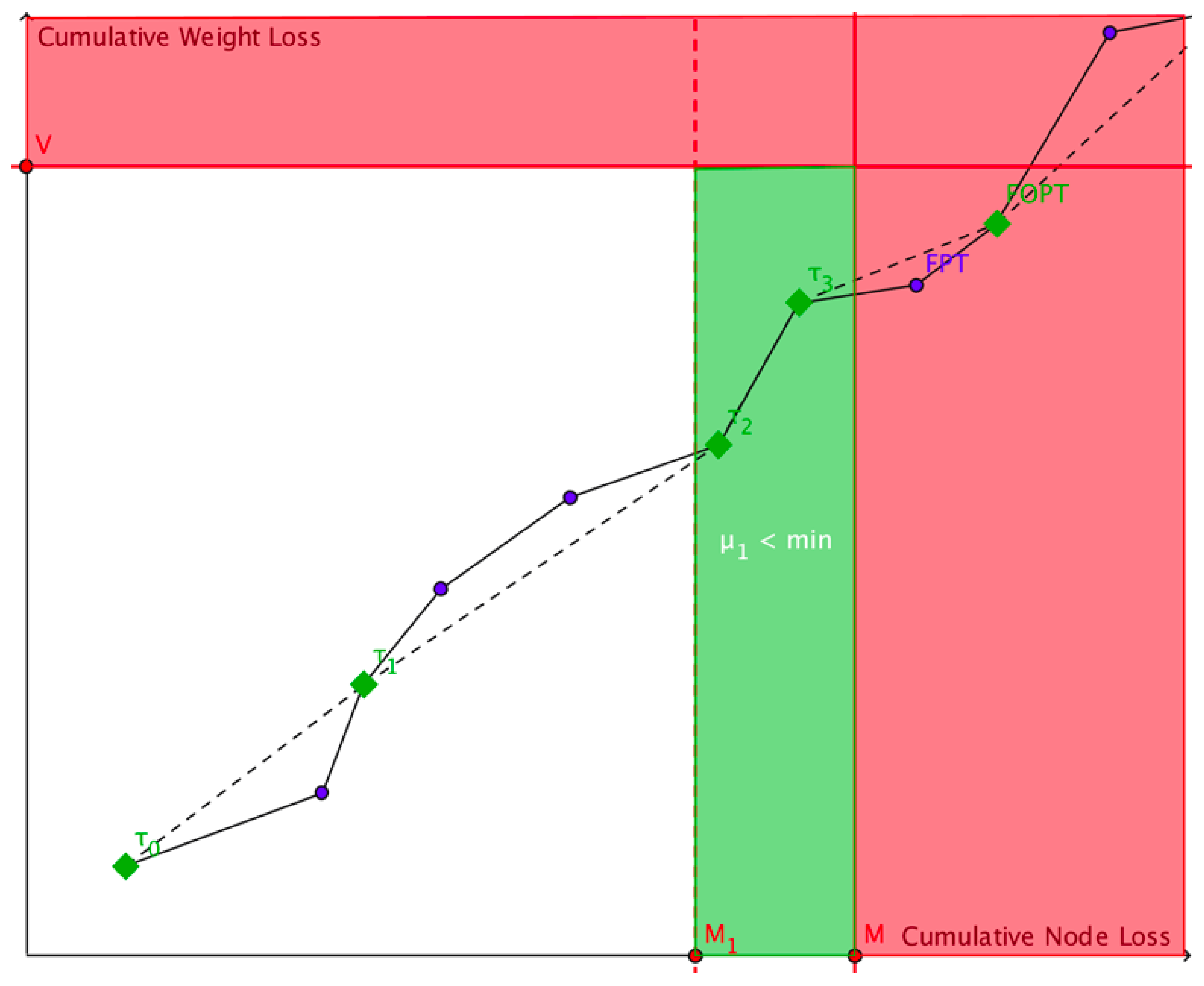
A realization of process $\mathcal{X}\otimes \mathcal{Y}\otimes \mathcal{T}$ of losses (defined in (26) above) in Figure 1 illustrates how it operates with respect to the introduced main and auxiliary thresholds. We can regard $\mathcal{X}\otimes \mathcal{Y}\otimes \mathcal{T}$ as a two-dimensional random walk on a random grid (rather than traditional lattice). We have a rectangular region formed of rectangular sectors in white, green, and red colors. In real-time the walker attempts to escape the white-green area at the first opportune time when the cumulative loss of nodes exceeds M or the cumulative weight loss exceeds V, whichever comes first. It leaves a polygonal path in blue and a cruder, observed, path in green. The walker enters the green area indicating that a lower threshold $M_1$ is crossed, while neither M nor V was. In reality, the green area can be empty with a positive probability.

In Figure 1, the underlying real-time process (the blue dots) represents the real-time incoming damages, which are observed only upon ${\tau }_k$’s (depicted by the green dots), where the $M_1$-observed-crossing occurs before the first observed passage time (FOPT) of M or V (i.e., there is an observation in the green area), at which the components of the process may or may not coincide with their values at the real-time FPT (first passage time).

The following assertion on functional ${\Phi }_{{\mu }_1<(\mu \wedge \nu )}$ about the escape parameters of random walk $\mathcal{X}\otimes \mathcal{Y}\otimes \mathcal{T}$ defined in (26) is an embellishment of the random walk model of Theorem 2 verbalized in the context of cyberattacks on a network, and can be found in [66] (Theorem 3.5).

Theorem 3.

The functional ${\Phi }_{{\mu }_1<(\mu \wedge \nu )}$ of the network damage on the confined sub-σ-algebra $\mathcal{F}\left(\Omega \right)\cap \left\{{\mu }_1<(\mu \wedge \nu )\right\}$ satisfies the formula

$$\begin{array}{c}\hfill {\Phi }_{{\mu }_1<(\mu \wedge \nu )}={\mathfrak{D}}_{xyw}\left(\left[{\varphi }_0^1-{\varphi }_0+\frac{{\phi }_0}{1-\phi }({\varphi }^1-\varphi )\right]\frac{{\xi }^1-\chi }{1-\psi }\right)\left(M_1,M,V\right)\end{array}$$

(38)

under the abbreviated notation in (39)–(44).

$$\begin{array}{cc}\hfill & \phi =\gamma \left(u_{0}u{\alpha }_0\alpha xy,v_0+v+{\beta }_0+\beta +w,{\theta }_0+\theta +h_0+h\right)\hfill \end{array}$$

(39)

$$\begin{array}{cc}& \varphi =\gamma \left(u{\alpha }_0\alpha xy,v+{\beta }_0+\beta +w,\theta +h_0+h\right)\hfill \end{array}$$

(40)

$$\begin{array}{cc}& {\varphi }^1=\gamma \left(u{\alpha }_0\alpha y,v+{\beta }_0+\beta +w,\theta +h_0+h\right)\hfill \end{array}$$

(41)

$$\begin{array}{cc}& \psi =\gamma \left({\alpha }_0\alpha y,{\beta }_0+\beta +w,h_0+h\right)\hfill \end{array}$$

(42)

$$\begin{array}{cc}& \chi =\gamma \left(\alpha y,\beta +w,h\right)\hfill \end{array}$$

(43)

$$\begin{array}{c}\hfill {\xi }^1=\gamma \left(\alpha ,\beta ,h\right)\end{array}$$

(44)

and expressions with 0 subscripts involve initial-jump functionals, e.g., ${\phi }_0$ is like φ except it uses ${\gamma }_0$ instead of γ.

Example 2.

In this example we will present fully explicit probabilistic results for a special case of the process with the $M_1$-auxiliary threshold, under the following five assumptions made in the context of network’s security.

• As previously, the attack times $\left\{t_1,t_2,\dots \right\}$ form a Poisson point process of rate λ.
• Inter-observation times are constant, i.e.,
  ${\Delta }_k={\tau }_k-{\tau }_{k-1}=c$ a.s., $L\left(\theta \right)=e^{-\theta c}$.
• Nodes lost per strike have an arbitrary finite discrete distribution, i.e., $P\{n_k=j\}=p_j$, $j=1,\dots ,R$ and PGF $g\left(z\right)={\sum }_{s=1}^R{p}_s{z}^s$, with p$=\left(p_1,\dots ,p_R\right)$
• Weight per node $w_{jk}\in \left[Gamma\left(\alpha ,\beta \right)\right]$, so we have LST $l\left(z\right)={\left(\frac{\beta }{z+\beta }\right)}^{\alpha }$.
• The initial functional ${\gamma }_0=1$ (i.e., zero initial damage).

We note that deterministic observations present more of a challenge than many random observations. The assumption on the number nodes destroyed in a single strike being bounded by R is analytically convenient but not too restrictive, because R can be made arbitrarily large. The general gamma distribution of weight of a single node is also pretty general.

Let $E\left[u^{N_{{\mu }_1}}{e}^{-v{W}_{{\mu }_1}}{e}^{-\theta {\tau }_{{\mu }_1}}{\mathbf{1}}_{\left\{{\mu }_1<(\mu \wedge \nu )\right\}}\right]$ be the ${\Phi }_{{\mu }_1<(\mu \wedge \nu )}$-marginal functional of walk’s position on the passage of threshold $M_1$ (see the green area in the figure above) with the main escape from set A not occurred. Then, the following holds formulated in the context of the cyberattack.

Under Assumptions 1–5, the joint transform of the number of lost nodes, their cumulative weight, and the first passage time of the crossing of $M_1$ preceding the first crossing of M or V (i.e., on the sub-σ-algebra $\mathcal{F}\left(\Omega \right)\cap \left\{{\mu }_1<(\mu \wedge \nu )\right\})$ satisfies the following formula [66]:

$$\begin{array}{cc}\hfill & {\Phi }_{{\mu }_1<(\mu \wedge \nu )}(1,u,1,1,0,v,0,0,\theta ,0,0)\hfill \\ & =E\left[u^{N_{{\mu }_1}}{e}^{-v{W}_{{\mu }_1}}{e}^{-\theta {\tau }_{{\mu }_1}}{\mathbf{1}}_{\left\{{\mu }_1<(\mu \wedge \nu )\right\}}\right]\hfill \\ & =e^{-c\left(\theta +\lambda \right)}\{\sum _{k=0}^{M_1-1}{u}^k{F}_k\left(\theta ,p\right)\sum _{m=0}^{M-1-k}{u}^m{E}_m\left(p\right){\left(\frac{\beta }{v+\beta }\right)}^{\alpha \left(k+m\right)}P\left(\alpha \left(k+m\right),\left(v+\beta \right)V\right)\hfill \\ & -\sum _{k=0}^{M_1-1}{u}^k{\left(\frac{\beta }{\beta +v}\right)}^{\alpha k}P\left(\alpha k,\left(v+\beta \right)V\right)\sum _{n=0}^k{E}_n\left(p\right)F_{k-n}\left(\theta ,p\right)\},\hfill \end{array}$$

(45)

where

$$\begin{array}{c}\hfill F_j\left(\theta ,\mathrm{p}\right)=\sum _{r=0}^{⌊\frac{R-1}{R}j⌋}{\left(c\lambda \right)}^{j-r}{\mathrm{Li}}_{-(j-r)}\left(e^{-c(\theta +\lambda )}\right)\sum _{\begin{array}{c}{\parallel \delta \parallel }_1=j\\ \left[R\right]·\delta =r+j\end{array}}\frac{p_1^{{\delta }_1}\cdots p_R^{{\delta }_R}}{{\delta }_1!\cdots {\delta }_R!},\end{array}$$

(46)

$\left[R\right]=\left(1,\dots ,R\right)$, $\delta =\left({\delta }_1,\dots ,{\delta }_R\right)\in {\mathbb{N}}_0^R$ (${\delta }_j\le R$for each j),

$$\begin{array}{c}\hfill E_j\left(p\right)=\sum _{r=0}^{⌊\frac{R-1}{R}j⌋}{\left(c\lambda \right)}^{j-r}\sum _{\begin{array}{c}{\parallel \delta \parallel }_1=j\\ \left[R\right]·\delta =r+j\end{array}}\frac{p_1^{{\delta }_1}\cdots p_R^{{\delta }_R}}{{\delta }_1!\cdots {\delta }_R!},\end{array}$$

(47)

Li${}_s\left(z\right)={\sum }_{k=1}^{\infty }{z}^k{k}^{-s}$ is the polylogarithm, which is numerically tractable for our domain $\left\{e^{-w}:\mathrm{Re}\left(w\right)>0\right\}$ with $s\in {\mathbb{Z}}_{\le 0}$, $P\left(x,y\right)=1-\frac{\Gamma \left(x,y\right)}{\Gamma \left(x\right)}$ is the upper regularized Gamma function, $\Gamma \left(x,y\right)$ is the incomplete gamma function, and $\Gamma \left(x\right)$ is the gamma function.

Remark 2.

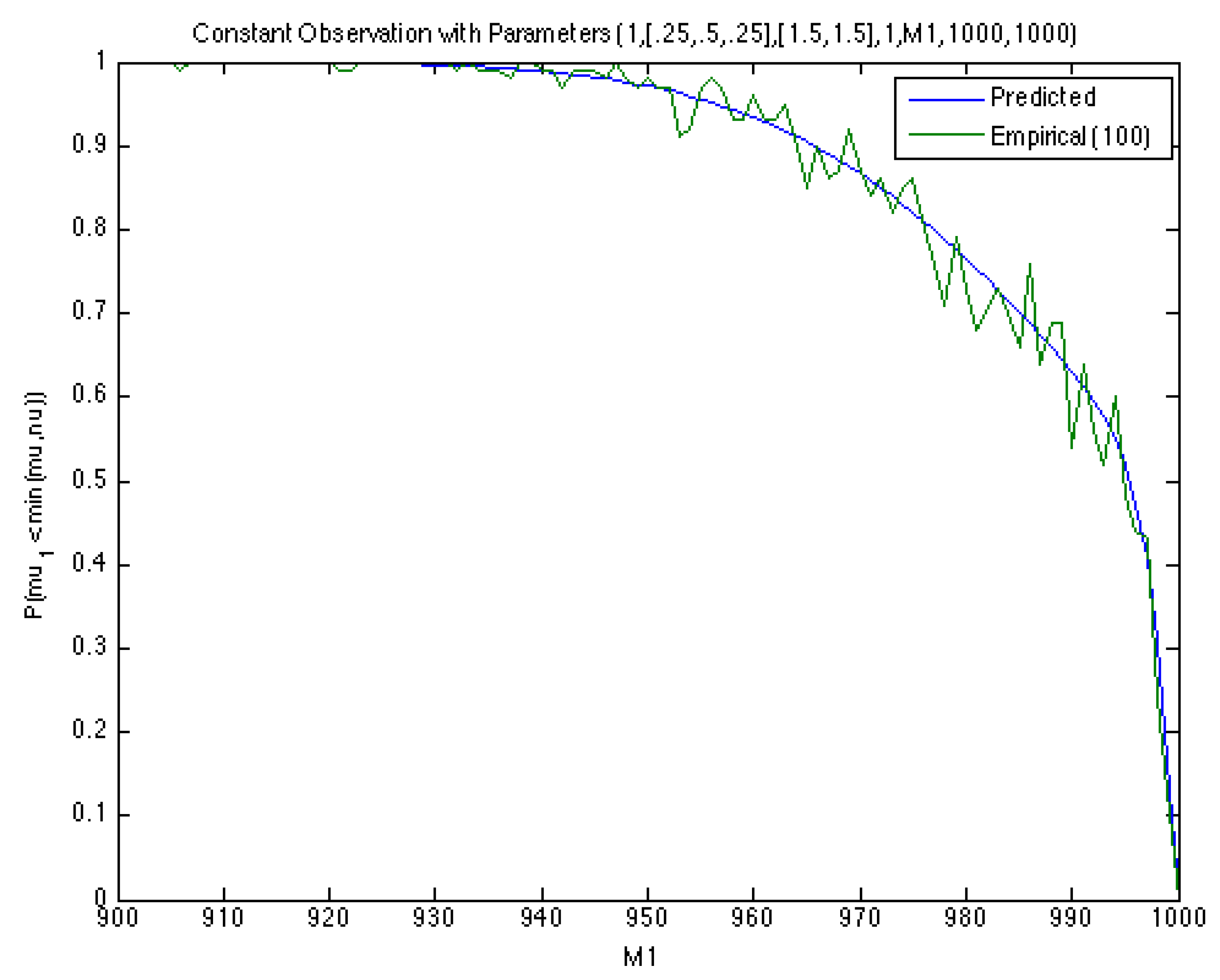
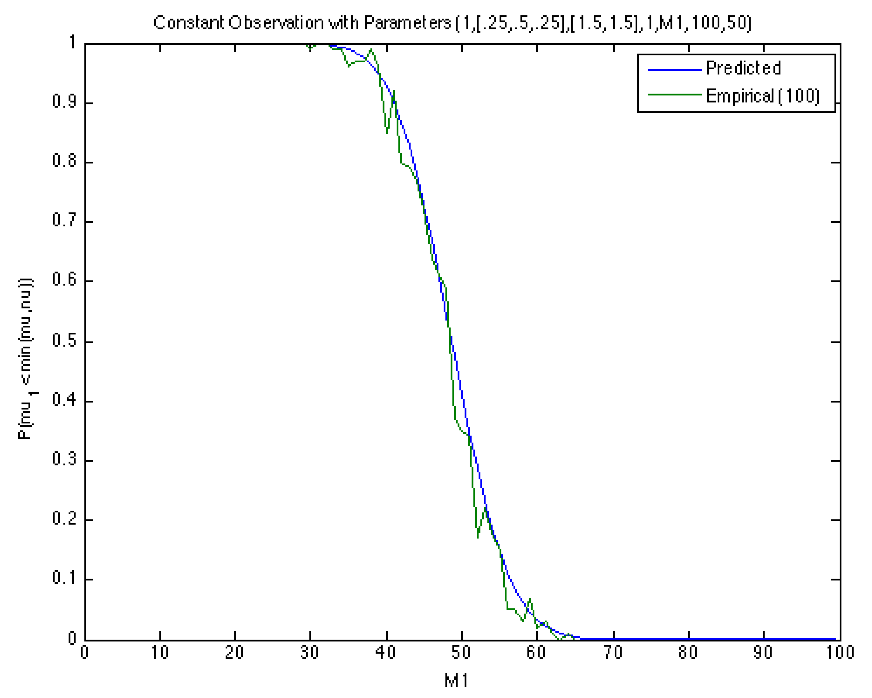
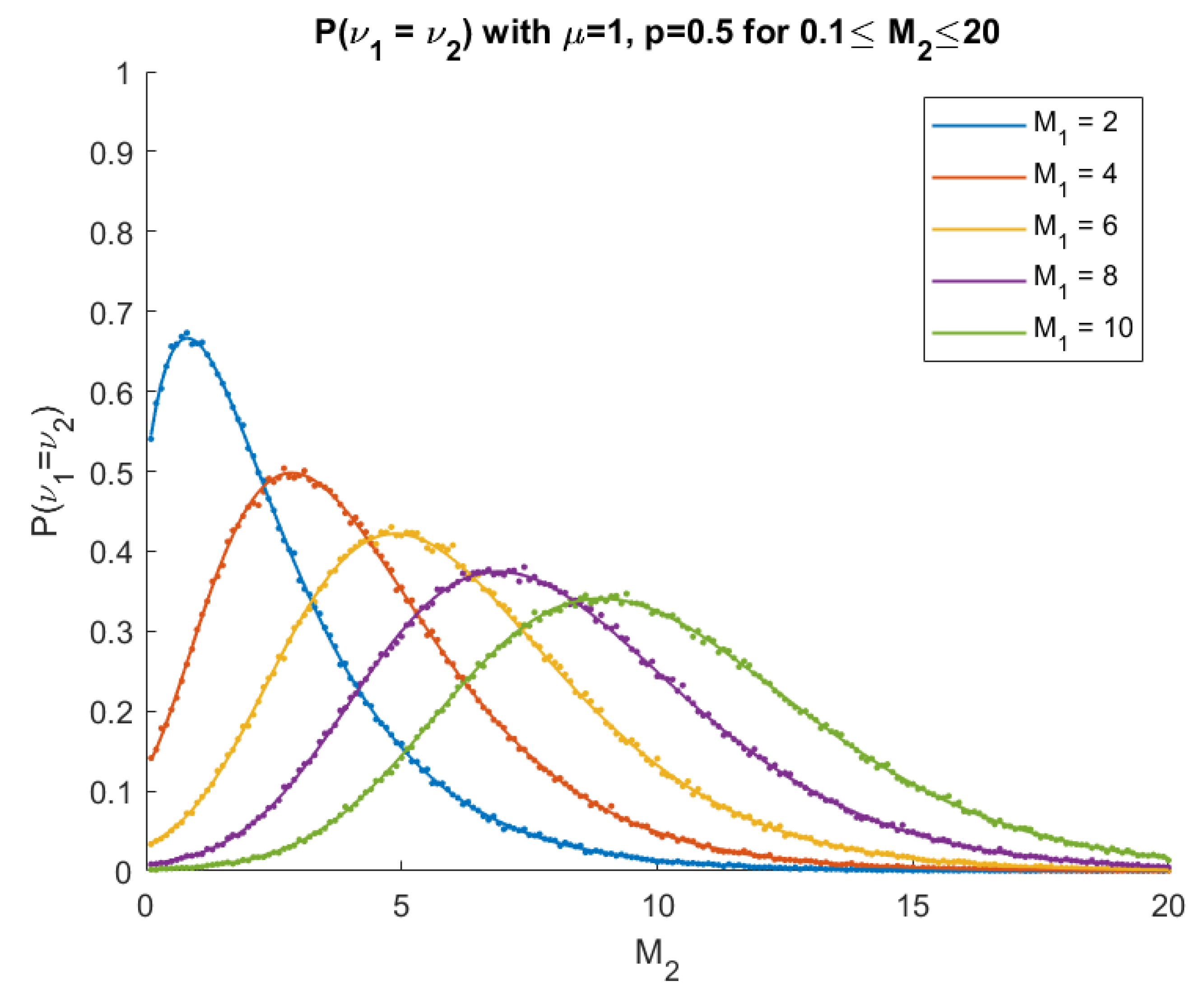
Through simulation of the process, we were able to produce some verification of the results via numerical examples presented in Figure 2 and Figure 3. For two sets of parameters of the process with $R=3$, $\left(\lambda ,[p_1,p_2,p_3],[\alpha ,\beta ],c,M_1,M,V\right)$, we generated 100 realizations of the process for each of a range of $M_1$ values and calculated the empirical probabilities $P\left\{{\mu }_1<(\mu \wedge \nu )\right\}$ for each:

Some current work by White [106] goes further and considers large networks with nodes connected by edges and the edges, rather than the nodes, have weights. Here, successive attacks take out a random number of nodes, which removes a random number of connected edges, each with a weight indicating its value to the network. The network enters into a critical state if losses of any of these three types accumulate beyond some pre-specified thresholds.

This is modeled through a Poisson random measure

$$\begin{array}{c}\hfill \eta =\mathcal{N}\otimes \mathcal{E}\otimes \mathcal{W}=\sum _{k\ge 1}\left(n_k,e_k,w_k\right){\epsilon }_{t_k},\end{array}$$

(48)

where $n_k$ nodes are incapacitated in the kth attack at time $t_k$, the jth node lost in the$k$th attack has $e_{jk}$ incident edges that go down, and the ith edge from the jth node lost in the kth attack has weight $w_{ijk}$, so we have

$$\begin{array}{cc}\hfill & e_k=\sum _{j=1}^{n_k}{e}_{jk}\hfill \end{array}$$

(49)

$$\begin{array}{cc}& w_k=\sum _{j=1}^{n_k}\sum _{i=1}^{e_{jk}}{w}_{ijk}\hfill \end{array}$$

(50)

This process is studied as above under delayed observation, so we consider the following random measure, similar to ((26)).

$$\begin{array}{c}\hfill \mathcal{X}\otimes \mathcal{Y}\otimes \mathcal{Z}\otimes \mathcal{T}=\sum _{n=0}^{\infty }\left(X_n,Y_n,Z_n\right){\epsilon }_{{\tau }_n},\end{array}$$

(51)

which is a three-dimensional random walk with mutually dependent marks $\left(X_n,Y_n,Z_n\right):\Omega \to \mathbb{N}\times \mathbb{N}\times {\mathbb{R}}_{+}$ and we define

$$\begin{array}{cc}\hfill & {\gamma }_0\left(u,v,w,h\right)=E\left[u^{\mathcal{N}\left({\tau }_0\right)}{u}^{\mathcal{E}\left({\tau }_0\right)}{e}^{-w\mathcal{W}\left({\tau }_0\right)-h{\tau }_0}\right]\hfill \end{array}$$

(52)

$$\begin{array}{cc}& \gamma \left(u,v,w,h\right)=E\left[u^{\mathcal{N}\left({\Delta }_1\right)}{v}^{\mathcal{E}\left({\Delta }_1\right)}{e}^{-w\mathcal{W}\left({\Delta }_1\right)-h{\Delta }_1}\right]\hfill \end{array}$$

(53)

We will define

$$\begin{array}{c}\hfill S_n=(N_n,E_n,W_n)=\left(\sum _{i=0}^n{X}_i,\sum _{i=0}^n{Y}_i,\sum _{i=0}^n{Z}_i\right).\end{array}$$

Here, there are three thresholds, $M_n$, $M_e$, $M_w$ for losses of nodes, edges, and weights, respectively, and three corresponding exit indices ${\rho }_n$, ${\rho }_e$, ${\rho }_w$ with $\rho ={\rho }_n\wedge {\rho }_e\wedge {\rho }_w$. We seek the functional

$$\begin{array}{cc}\hfill \Phi & =\Phi \left(\xi ,u_0,u,v_0,v,w_0,w,h_0,h\right)\hfill \\ & =E\left[{\xi }^{\rho }{u}_0^{N_{\rho -1}}{u}^{N_{\rho }}{v}_0^{E_{\rho -1}}{v}^{E_{\rho }}{e}^{-w_0{W}_{\rho -1}-w{W}_{\rho }}{e}^{-h_0{\tau }_{\rho -1}-h{\tau }_{\rho }}\right],\hfill \end{array}$$

(54)

which is much like the functional (29) from Theorem 2, except it includes some extra terms for the edge losses upon the exit, $E_{\rho -1}$ and $E_{\rho }$, and also includes a term ${\xi }^{\rho }$ corresponding to a probability-generating function of the number of observations before the network enters into its critical state.

The functional has been derived through a procedure similar to Theorem 2 above, although it is a bit more difficult since this problem is three-dimensional and the weight lost per attack is more complex. To accomplish this, we can use the operator

$$\begin{array}{c}\hfill {\mathfrak{D}}_{xyz}\left(·\right)\left(p,q,r\right)=\mathcal{L}{\mathcal{C}}_z^{-1}\circ {\mathcal{D}}_y^q\circ {\mathcal{D}}_x^p\left(·\right)\left(r\right)\end{array}$$

(55)

Theorem 4.

The functional Φ satisfies the formula

$$\begin{array}{cc}\hfill \Phi =& {\mathfrak{D}}_{xyz}[{\gamma }_0\left(u,v,w,h\right)-{\gamma }_0\left(ux,vx,w+z,h\right)\hfill \\ & +\frac{\xi {\gamma }_0}{1-\xi \gamma }\left(\gamma \left(u,v,w,h\right)-\gamma \left(ux,vy,w+z,h\right)\right)]\left(M_n,M_e,M_w\right),\hfill \end{array}$$

(56)

where

$$\begin{array}{cc}\hfill & {\gamma }_0={\gamma }_0\left(u_{0}ux,v_{0}vy,w_0+w+z,h_0+h\right)\hfill \end{array}$$

(57)

$$\begin{array}{cc}& \gamma =\gamma \left(u_{0}ux,v_{0}vy,w_0+w+z,h_0+h\right)\hfill \end{array}$$

(58)

It is easy to draw many parallels between the functionals in Theorem 2 [65] and Theorem 4 [106], which is suggestive of some structure that can extend to higher dimensional results, as has recently been shown and will be outlined in Section 5 below.

4. Time Insensitive Random Walk and Applications

In summary, the random walk analysis surveyed in Section 2 and Section 3 is referred to as time insensitive analysis and the associate random walk is time insensitive. See Agarwal, Dshalalow, and O’Regan [107], Agarwal and Dshalalow [108], Dshalalow [56,57], and Dshalalow and Liew [58,59,60]. It pertains to the fact that the random walk process we analyzed so far cannot be associated with continuous time information, say $S\left(t\right)$ giving us the status of the walk at any time t simultaneously with $S_{\nu },t_{\nu }$ and other escape parameters within interval $\left[0,t\right]$. Of course, we can pull out some probabilistic information about the location of ${\tau }_{\nu }$ such as $P\left\{t_{\nu }\le t\right\}$ or $P\left\{t_{\nu }\in B\right\}$ and likewise $P\left\{S_{\nu }\in R\right\}$ or for that matter, the finite-dimensional distribution of S${}_{\nu }$. However, this still falls short of the time continuous information $S\left(t\right)$ on the walk that is very important in control theory. It was very obvious that with our efforts to embed an auxiliary control level $M_1$ prior to the main escape, we make up for the lack of $S\left(t\right)$. In the forthcoming sections we will address this issue and present time sensitive walks which appear to provide us with a bulk of additional information, but at a cost, because the insensitive analysis is tamer.

We return to this topic later, but for now we would like to present some applications of the insensitive walks beyond the cyberattack models in Section 3.

Consider the random walk

$$\begin{array}{c}\hfill \mathcal{S}=\mathcal{A}\otimes \mathcal{P}=\sum _{k=0}^{\infty }\left({\mathbf{A}}_k,{\mathbf{P}}_k\right){\epsilon }_{t_k},\end{array}$$

valued in ${\mathbb{N}}^d\times {\mathbb{R}}^l$ such that

$$\begin{array}{c}\hfill \left({\mathcal{A}}_n,{\mathcal{P}}_n\right)=\left(\sum _{k=0}^n{\mathbf{A}}_k,\sum _{k=0}^n{\mathbf{P}}_k\right)\end{array}$$

is the position of the walker on the associated random grid. From this position, the walker jumps to position $\left({\mathcal{A}}_{n+1},{\mathcal{P}}_{n+1}\right)$. Here,

$$\begin{array}{cc}\hfill & {\mathbf{A}}_k=\left(A_{k1},\cdots ,A_{kd}\right),\hfill \end{array}$$

(59)

$$\begin{array}{cc}& {\mathbf{P}}_k=\left(P_{k1},\cdots ,P_{kl}\right),\hfill \end{array}$$

(60)

while

$$\begin{array}{cc}\hfill & {\mathcal{A}}_n=\left({\alpha }_{n1}=\sum _{k=0}^n{A}_{k1},\cdots ,{\alpha }_{nd}=\sum _{k=0}^n{A}_{kd}\right)\hfill \end{array}$$

(61)

$$\begin{array}{cc}& {\mathcal{P}}_n=\left({\pi }_{n1}=\sum _{k=0}^n{P}_{k1},\cdots ,{\pi }_{nl}=\sum _{k=0}^n{P}_{kl}\right).\hfill \end{array}$$

(62)

The objective is to investigate time and the position of the walker when its component $\mathcal{A}$ escapes from rectangle $A={\prod }_{i=1}^d{R}_i\subseteq {\mathbb{N}}^d$. Often of main interest is the position of the walker in ${\mathbb{R}}^l$. Component $\mathcal{A}$ of $\mathcal{S}$ is called the active, while $\mathcal{P}$ is passive implying that in our case, only $\mathcal{A}$ is contained, while $\mathcal{P}$ is unrestricted. Note that, unlike the previous assumptions in Section 2 and Section 3, the walk in ${\mathbb{R}}^l$ runs in all directions along a randomly generated grid. However, the escape is determined by the projection $\left[{\mathbb{N}}^d\times {\mathbb{R}}^l,{\mathbb{N}}^d,\pi \right]$ of the position of the walker relative to set A. Here $\pi$ is defined as the projection map from ${\mathbb{N}}^d\times {\mathbb{R}}^l$ to ${\mathbb{N}}^d$.

In a nutshell, the escape coordinates in ${\mathbb{N}}^d\times {\mathbb{R}}^l$ are determined by the time and location of the active components $\mathcal{A}$ of the walker upon their first crossing of A. Obviously, the exit from A occurs when at least one of the active entries ${\alpha }_{nj}$ crosses $R_j$ of rectangle R.

The exit index is defined as

$$\begin{array}{c}\hfill \rho =inf\left\{n:{\mathcal{A}}_n\in A^c\right\},\end{array}$$

(63)

implying that $t_{\rho }$ is the first passage time and ${\mathcal{S}}_{\rho }=({\mathcal{A}}_{\rho },{\mathcal{P}}_{\rho })$ is the global location of the walker in $A\times {\mathbb{R}}^l$ upon $\mathcal{A}$’s escape from set A.

Before we continue with more formalism, let us bring up a situation that led to the above model.

Example 3.

Suppose an agent decides whether or not to short an option on some stock S${}_1$ he does not own. In the event he decides to short the option, he wonders if he is to acquire the stock or not to dependent on the stock’s chance to hit the strike price. In this case, if the agent does not own the stock, while it hits the strike price and the option holder will exercise the contract, he will have to deliver the stock and thus buy it at a market price. This particular example does not demonstrate how to find the probability that the stock described by a random walk process will cross the threshold determined by the strike price, but it will give the functional of the first passage time when the stock drops for the first time or when its increment will increase above some level $M_1$. This can be used as an initial information for the stock to run its further path. This information can also be used whenever one decides whether or not to buy a volatile stock. Now, the prediction about the first drop or sharp increase can be refined by adhering to stock S${}_1$ yet another stock, say S${}_2$, which is proved to be well correlated with S${}_1$. Then, instead of a scrutiny on stock S${}_1$ alone, we can mix S${}_1$ and S${}_2$ to see whichever of the two will come first to drop or rise. The prediction can be more accurate.

In a similar situation, suppose an owner of a stock portfolio is interested to extend or update it with more stocks. A diversification is a common strategy. Another strategy is to mix a portfolio with longs and shorts. Suppose the agent would want to know whether to long or short just two stocks dependent on what direction they may take. For instance, if a sharp drop occurs, it could be a signal of price decline; if a significant rise takes place without any economical reasons, it could be an indication of overpricing that would present another risk to the stock owner. In this case, the owner would also like to predict the moment either the first drop or a significant rise is to happen (which we will associate with the first passage or exit time). Then, if necessary, shorting the two stocks, the agent would be able to minimize risk, optimize the respective portfolio’s performance and thus attain a higher return on his investment.

In the context of the above notation, ${\pi }_{n1}$ and ${\pi }_{n2}$ give the prices of the two stocks upon reference times $t_n,n=1,2,\dots$ so that $P_{n1}$ and $P_{n2}$ are increments of the stock price changes between their respective subintervals $(t_{n-1},t_n],$ where $t_0=0$. We would like to emphasize that because the stock prices periodically change their directions, the named increments are real-valued r.v.’s, rather than positive and thus the stock prices are not monotone, in contrast with monotone components of Section 2 and Section 3.

Introduce four auxiliary active components

$$\begin{array}{cc}\hfill & A_{n1}=\left\{\begin{array}{cc}0,& P_{n1}\ge 0\\ 1,& P_{n1}<0\end{array}\right.\hfill \end{array}$$

(64)

$$\begin{array}{cc}& A_{n2}=\left\{\begin{array}{cc}0,& P_{n2}\ge 0\\ 1,& P_{n2}<0\end{array}\right.\hfill \end{array}$$

(65)

$$\begin{array}{c}\hfill A_{n3}=\left\{\begin{array}{cc}0,& P_{n1}<M_1\\ 1,& P_{n1}\ge M_1\end{array}\right.\end{array}$$

(66)

$$\begin{array}{c}\hfill A_{n4}=\left\{\begin{array}{cc}0,& P_{n2}<M_2\\ 1,& P_{n2}\ge M_2\end{array}\right.\end{array}$$

(67)

that follow the evolution of two questionable stocks’ prices. Now since the stock price changes are not monotone sequences, we associate them with passive components whereas the auxiliary components of (64)–(67) are monotone.

Now while stock S${}_i$’s price appreciates, $A_{ki}=0,k=1,2,\dots ,$ resulting in $\left({\alpha }_{n1},{\alpha }_{n2}\right)=\left(0,0\right),n=1,2,\dots ,i=1,2$. When at some $t_n,$at least one of the two stock prices drops for the first time, we will see $({\alpha }_{n1},{\alpha }_{n2})=\left(0,1\right)$ or $\left(1,0\right),$ or $\left(1,1\right)$. The other two active components of $\mathcal{A}$ will watch similarly behaving rising trends of the two stocks as per (66) and (67).

Thus, setting the rectangle $A=\{0,R_1\}\times \{0,R_2\}\times \{0,R_3\}\times \{0,R_4\}$ we can predict the trend of the two stocks to appreciate or dive and suggest a longing or shorting strategy of acquiring stock portfolio. For example, crossing $R_1$ or $R_2$ at $t_{\rho }$ points to changing direction of the respective stock prices from rising to dropping. On the other hand, crossing $R_3$ or $R_4$ points to a solid gain in prices that suggests longing rather than shorting the stocks. A mixed trend speaks of unwanted volatility.

Back to the general case, we introduce the functional

$$\begin{array}{cc}\hfill {\Phi }_{\rho }& ={\Phi }_{\rho }\left(\xi ,\mathit{u},\mathit{v},\mathbf{\eta },\mathbf{\xi },\vartheta ,\theta \right)\hfill \\ & =E\left[{\xi }^{\rho }{u}_1^{{\alpha }_{\rho 1-1}}\cdots u_d^{{\alpha }_{\rho d-1}}{v}_1^{{\alpha }_{\rho 1}}\cdots v_d^{{\alpha }_{\rho d}}\times e^{i\mathbf{\eta }·{\mathcal{P}}_{\rho -1}+i\xi ·{\mathcal{P}}_{\rho }-\vartheta t_{\rho -1}-\theta t_{\rho }}\right]\hfill \end{array}$$

(68)

such that u $=\left(u_1,\cdots ,u_d\right)$, v$(v_1,\cdots ,v_d)\in {\mathbb{C}}^d$ with $u_i,v_i\in \overline{B}\left(0,1\right)$ for $i=1,\cdots ,d$, $\mathbf{\eta },\mathbf{\xi }\in {\mathbb{R}}^l$, and $\vartheta ,\theta \in {\mathbb{C}}_{+}$. (i.e., Re$\left(\vartheta \right)\ge 0$ and Re$\left(\theta \right)\ge 0$.)

This functional includes familiar escape and pre-escape parameters. One of the utilities of pre-escape parameters, at least in the context of stock prices or option trading, is to predict the highest stock price, say before a drop or a second drop or sharp drop.

Next we have the multivariate version of the $\mathcal{D}$-operator defined as

$$\begin{array}{c}\hfill {\mathcal{D}}_{\mathrm{x}}^{\mathrm{R}}={\mathcal{D}}_{x_1}^{R_1}\circ \dots \circ {\mathcal{D}}_{x_d}^{R_d}\end{array}$$

(69)

such that ${\mathcal{D}}_{x_i}^{R_i}\left\{\phi \left(\mathrm{x}\right)\right\}={lim}_{x_i\to 0}\frac{1}{R_i!}\frac{{\partial }^{R_i}}{\partial x^{R_i}}\left[\frac{1}{1-x_i}\phi \left(\mathbf{x}\right)\right]$, where $\mathbf{R}=\left(R_1,\dots ,R_d\right)$, $\mathbf{x}=\left(x_1,\dots ,x_d\right)\in {\mathbb{C}}^d$, $x_i\in B(0,1)$ for $i=1,\dots ,d$, and $\phi$ is analytic at 0 with respect to each $x_1,\dots ,x_d$.

Theorem 5.

The functional ${\Phi }_{\rho }$ satisfies the following formula.

$$\begin{array}{cc}\hfill {\Phi }_{\rho }={\mathcal{D}}_{\mathit{x}}^{\mathrm{R}-\mathit{1}}[& {\gamma }_0\left(\mathit{v};\mathit{\xi },\theta \right)-{\gamma }_0\left(\mathit{x}\circ \mathit{v};\mathit{\xi },\theta \right)\hfill \\ & +{\gamma }_0\left(\mathit{x}\circ \mathit{u}\circ \mathit{v};\eta +\xi ,\vartheta +\mathit{\theta }\right)\frac{\mathit{\xi }\gamma \left(\mathit{v};\mathit{\xi },\theta \right)-\gamma \left(\mathit{x}\circ \mathit{v};\mathit{\xi },\theta \right)}{1-\xi \gamma \left(\mathit{x}\circ \mathit{u}\circ \mathit{v};\eta +\mathit{\xi },\vartheta +\theta \right)}]\hfill \end{array}$$

(70)

where

$$\begin{array}{cc}\hfill & {\gamma }_0\left(\mathit{u};\eta ,\vartheta \right)=E\left[u_1^{A_{01}}\cdots u_d^{A_{0d}}{e}^{i\eta ·P_0-\vartheta t_0}\right]\hfill \end{array}$$

(71)

$$\begin{array}{cc}& \gamma \left(\mathit{u};\eta ,\vartheta \right)=E\left[u_1^{A_{11}}\cdots u_d^{A_{1d}}{e}^{i\eta ·P_1-\vartheta (t_1-t_0)}\right]\hfill \end{array}$$

(72)

andu∘vis the Hadamard product of vectorsuandv.

We note that the functionals γ and ${\gamma }_0$ are supposed to be known or they can be obtained. We revisit Example 3 about stocks trading.

Example 4.

In the context of Example 3 consider a special case when an agent observes two stocks with some initial constant prices $P_{01},P_{02}$ at the beginning, under assumption that $t_0=0$. Because $P_{01}$ and $P_{02}$ are positive, $A_{01}=A_{02}=0$. It makes sense to set $P_{01}<M_1$ and $P_{02}<M_2,$ thereby setting $A_{03}=A_{04}=0$ as well. Thus we have $\mathit{u}=\mathbf{1}$, so

$$\begin{array}{c}\hfill {\gamma }_0\left(\mathbf{1};\eta ,0\right)=e^{i\left({\eta }_1{P}_{01}+{\eta }_2{P}_{02}\right)}=g_0\left(\eta \right)\end{array}$$

(73)

is a fixed constant.

Next, the agent wants to predict the first instant $t_{\rho }$ when at least one of the four events takes place: Stocks prices of S${}_1$ or S${}_2$ drop for the first time after appreciating, or with their increments P$=\left(P_1,P_2\right)$ spike above $M_1$ or $M_2$. If any of these events occur at time $t_{\rho }$, they will turn $P_{\rho 1}$ or $P_{\rho 2}$ negative and thus $A_{\rho 1}$ or $A_{\rho 2}=1,$ or $P_{\rho 1}\ge M_1$ or $P_{\rho 2}\ge M_1$ and thus $A_{\rho 3}$ or $A_{\rho 4}=1$. Therefore, $A={\left\{0,1\right\}}^4$ and $\mathbf{R}=\left(1,1,1,1\right)$.

We need to figure out

$$\begin{array}{cc}\hfill \gamma \left(\mathit{u};\eta ,\vartheta \right)& =E\left[u_1^{A_{11}}\cdots u_d^{A_{14}}{e}^{i\eta ·P_1-\vartheta t_1}\right]\hfill \\ & =E\left[e^{i\eta ·P_1-\vartheta t_1}{\mathbf{1}}_{\left\{\mathbf{0}\le P_1<\mathbf{M}\right\}}\right]+E\left[u_1{e}^{i\eta ·P_1+\vartheta t_1}{\mathbf{1}}_{\left\{P_{11}<0,0\le P_{12}<M_2\right\}}\right]\hfill \\ & +E\left[u_2{e}^{i\eta ·P_1-\vartheta t_1}{\mathbf{1}}_{\left\{0\le P_{11}<M_1,P_{12}<0\right\}}\right]+E\left[u_3{u}_4{e}^{i\eta ·P_1-\vartheta t_1}{\mathbf{1}}_{\left\{P_1\ge \mathrm{M}\right\}}\right]\hfill \\ & +E\left[u_4{e}^{i\eta ·P_1-\vartheta t_1}{\mathbf{1}}_{\left\{0\le P_{11}<M_1,P_{12}\ge M_2\right\}}\right]+E\left[u_1{u}_4{e}^{i\eta ·P_1-\vartheta t_1}{\mathbf{1}}_{\left\{P_{11}<0,P_{12}\ge M_2\right\}}\right]\hfill \\ & +E\left[u_2{u}_3{e}^{i\eta ·P_1-\vartheta t_1}{\mathbf{1}}_{\left\{P_{11}\ge M_1,P_{12}<0\right\}}\right]+E\left[u_1{u}_2{e}^{i\eta ·P_1-\vartheta t_1}{\mathbf{1}}_{\left\{P_1<\mathbf{0}\right\}}\right]\hfill \\ & +E\left[u_3{e}^{i\eta ·P_1-\vartheta t_1}{\mathbf{1}}_{\left\{P_{11}\ge M_1,0\le P_{12}<M_2\right\}}\right]\hfill \end{array}$$

(74)

where $\mathbf{M}=\left(M_1,M_2\right)$. This can be calculated dependent on the choice of distributions of Pand $t_1$. (With position independent marking, that is, assuming Pand $t_1$ independent, the computation can be straightforward.) Now applying Theorem 5, we have

$$\begin{array}{cc}\hfill {\Phi }_{\rho }& ={\mathcal{D}}_{\mathit{x}}^{\mathbf{0}}[{\gamma }_0\left(\mathit{v};\mathit{\xi },\theta \right)-{\gamma }_0\left(\mathit{x}\circ \mathit{v};\mathit{\xi },\theta \right)\hfill \\ & +{\gamma }_0\left(\mathit{x}\circ \mathit{u}\circ \mathit{v};\mathit{\eta }+\mathit{\xi },\vartheta +\theta \right)\frac{\mathit{\xi }\gamma \left(\mathit{v};\mathit{\xi },\theta \right)-\gamma \left(\mathit{x}\circ \mathit{v};\mathit{\xi },\theta \right)}{1-\mathit{\xi }\gamma \left(\mathit{x}\circ \mathit{u}\circ \mathit{v};\mathit{\eta }+\mathit{\xi },\vartheta +\theta \right)}]\hfill \\ & =g_0\left(\mathit{\eta }+\mathit{\xi }\right)\frac{\mathit{\xi }\gamma \left(\mathit{v};\mathit{\xi },\theta \right)-\gamma \left(\mathbf{0};\mathit{\xi },\theta \right)}{1-\mathit{\xi }\gamma \left(\mathbf{0};\mathit{\eta }+\mathit{\xi },\vartheta +\theta \right)}\hfill \end{array}$$

(75)

For example, the most explicit functional is the marginal distribution of the exit index ρ (which is the predicted observation number from $1,2,\cdots$ when the above mentioned events take place). Thus, the pgf of ρ reads

$$\begin{array}{cc}\hfill & E{\xi }^{\rho }={\Phi }_{\rho }\left(\mathit{\xi },\mathbf{1},\mathbf{1},\mathbf{0},\mathbf{0},0,0\right)=\frac{\xi \gamma \left(\mathbf{1};\mathbf{0},0\right)-\gamma \left(\mathbf{0};\mathbf{0},0\right)}{1-\xi \gamma \left(\mathbf{0};\mathbf{0},0\right)}=\xi \frac{1-a}{1-\xi a},\hfill \end{array}$$

(76)

where

$$\begin{array}{c}\hfill a=\gamma \left(\mathbf{0},\mathbf{0},0\right)=P\left\{\mathbf{0}\le P_1<\mathbf{M}\right\}\end{array}$$

(77)

In particular, the mean of ρ is

$$\begin{array}{c}\hfill E\rho =\frac{1}{1-a}\end{array}$$

(78)

Next, the marginal LST of $t_{\rho -1}$ is

$$\begin{array}{cc}\hfill & {\Phi }_{\rho }\left(1,\mathbf{1},\mathbf{1},\mathbf{0},\mathbf{0},\vartheta ,0\right)=E{e}^{-\vartheta {\tau }_{\rho -1}}=\frac{1-\gamma \left(\mathbf{0},0,0\right)}{1-\gamma \left(\mathbf{0},0,\vartheta \right)}=\frac{1-a}{1-a\left(\vartheta \right)},\hfill \end{array}$$

(79)

where

$$\begin{array}{c}\hfill a\left(\vartheta \right)=E{e}^{-\vartheta t_1}{\mathbf{1}}_{\left\{\mathbf{0}\le P_1<\mathbf{M}\right\}}=aE{e}^{-\vartheta t_1}=aq\left(\vartheta \right)\end{array}$$

(80)

(if with position independent marking).

Thus, under the position independent marking assumption (that is price variations are independent of the time increments, the marginal transform of the highest portfolio price before at least one of the two stocks drops or spikes is

$$\begin{array}{c}\hfill E{e}^{-\vartheta t_{\rho -1}}=\frac{1-a}{1-aq\left(\vartheta \right)},\end{array}$$

(81)

implying that the mean time prior to one of these events is

$$\begin{array}{c}\hfill E{t}_{\rho -1}=\frac{aE{t}_1}{1-a}.\end{array}$$

(82)

5. Higher Dimensional Random Walks

Consider a random measure $\left(\mathcal{S},\mathcal{T}\right)={\sum }_{n=0}^{\infty }{\mathbf{x}}_n{\epsilon }_{{\tau }_n}$, where ${\mathbf{x}}_n=\left({\mathcal{X}}_n,{\mathcal{Y}}_n\right)\in {\mathbb{R}}_{+}^k\times {\mathbb{R}}^m$, and the corresponding delayed renewal process

$$\begin{array}{c}\hfill {\mathbf{S}}_n=\left({\mathcal{A}}_n,{\mathcal{P}}_n\right)=\left(\sum _{i=0}^n{\mathcal{X}}_i,\sum _{i=0}^n{\mathcal{Y}}_i\right),\end{array}$$

(83)

where ${\mathcal{A}}_n=\left(A_n^1,\dots ,A_n^k\right)$ and ${\mathcal{P}}_n=\left(P_n^1,\dots ,P_n^m\right)$. Unlike any model considered previously, some components of the jumps, the passive components ${\mathcal{Y}}_n$, are permitted to be negative.

Given the rectangle $A=\left[0,L_1\right]\times \cdots \times \left[0,L_k\right]\times {\mathbb{R}}^m,$ where $L=\left(L_1,\dots ,L_k\right)\in {\mathbb{R}}_{+}^k,$ we are interested in the escape parameters upon walker’s exit from set A. Namely,

$$\begin{array}{c}\hfill {\nu }_i=inf\{n\ge 0:A_n^i>L_i\}\end{array}$$

(84)

are the exit indices, and we focus on the first exit index

$$\begin{array}{c}\hfill \rho =inf\left\{{\nu }_i:i=1,\cdots ,k\right\}=inf\left\{n\ge 0:{\mathrm{S}}_n\notin A\right\}.\end{array}$$

(85)

As seen in a prior section, Dshalalow and Liew [59,60] derived a functional containing the pre-exit and post-exit non-negative active components ${\mathcal{A}}_{\rho -1}$ and ${\mathcal{A}}_{\rho }$ as well as real-valued passive components ${\mathcal{P}}_{\rho -1}$ and ${\mathcal{P}}_{\rho }$,

$$\begin{array}{cc}\hfill {\Phi }_{\rho }& ={\Phi }_{\rho }(\xi ,\alpha ,\varphi ,\beta ,\psi )=E{\xi }^{\rho }{e}^{-\alpha ·{\mathcal{A}}_{\rho -1}}{e}^{i\varphi ·{\mathcal{P}}_{\rho -1}}{e}^{-\beta ·{\mathcal{A}}_{\rho }}{e}^{i\psi ·{\mathcal{P}}_{\rho }},\hfill \end{array}$$

(86)

where $\mathit{\xi }\in \overline{B}(0,1)$, each component of $\alpha$, $\beta \in {\mathbb{C}}^k$ have non-negative real parts, and $\varphi$, $\psi \in {\mathbb{C}}^m$.

A new work by White [109] departs from the works above to derive a general formula for the probability of an arbitrary weak ordering of threshold crossings, a question of practical interest in numerous applications outlined above related to stochastic network defense, queueing theory, finance, and actuarial sciences.

In particular, a weak ordering of the exit indices ${\nu }_1$, ..., ${\nu }_k$ is a member of the set

$$\begin{array}{c}\hfill \mathcal{W}=\left\{\left\{{\nu }_{p\left(1\right)}⪯{\nu }_{p\left(2\right)}⪯\cdots ⪯{\nu }_{p\left(k\right)}\right\}:p\mathrm{is}\mathrm{a}\mathrm{permutation}\mathrm{of}\left\{1,\cdots ,k\right\}\right\},\end{array}$$

(87)

where each ⪯ is fixed to be either = or <. Without loss of generality, each $W\in \mathcal{W}$ may be represented as

$$\begin{array}{c}\hfill W=\left\{{\nu }_1=\cdots ={\nu }_{s_1}<{\nu }_{s_1+1}=\cdots ={\nu }_{s_2}<\cdots <{\nu }_{s_{n-1}+1}=\cdots ={\nu }_{s_n}\right\},\end{array}$$

(88)

keeping in mind some permutation may be applied to the indices of the $\nu$’s. The proofs within Dshalalow [40] and Dshalalow and Liew [59,60] among others partition the sample space into $\mathcal{W}$ and derive functionals of the form

$$\begin{array}{cc}\hfill {\Phi }_W& ={\Phi }_W(\xi ,\alpha ,\varphi ,\beta ,\psi )=E{\xi }^{\rho }{e}^{-\alpha ·{\mathcal{A}}_{\rho -1}}{e}^{i\varphi ·{\mathcal{P}}_{\rho -1}}{e}^{-\beta ·{\mathcal{A}}_{\rho }}{e}^{i\psi ·{\mathcal{P}}_{\rho }}{\mathbf{1}}_W\hfill \end{array}$$

(89)

for each weak ordering $W\in \mathcal{W}$ separately for $k\le 4$ before adding them to find ${\Phi }_{\rho }$. Note that a special case of ${\Phi }_W$ is

$$\begin{array}{c}\hfill {\Phi }_W(1,\mathbf{0},\mathbf{0},\mathbf{0},\mathbf{0})=E{\mathbf{1}}_W=P\left(W\right),\end{array}$$

(90)

the probability of the weak ordering W occurring.

This could be done manually for $k\ge 5$ in principle, but it is impractical. $\mathcal{W}$ contains all permutations of $\{{\nu }_1,\cdots ,{\nu }_k\}$ with strict inequalities, i.e., where threshold crossings occur at distinct times, which is already $k!$elements. Further, $\mathcal{W}$ also contains many other weak orderings because arbitrary subsets of the threshold crossings may occur upon the same jump of the process. It turns out the cardinalities of $\mathcal{W}$ for dimension k correspond to the Fubini numbers (or ordered Bell numbers): 1, 3, 13, 75, 541, 4683, 47,293, ... Deriving 75 ${\Phi }_W$ functionals for dimension four was feasible but took quite a lot of effort. Some experimentation has shown that moving up to seven dimensions on a similar problem is time-consuming but feasible with an automated procedure with a consumer-grade computer, and a few more dimensions should work on more substantial hardware, but it soon becomes infeasible regardless of computational resources.

The main result of White [109] takes an alternate path and generalizes the derivation of an arbitrary $P\left(W\right)$ in any finite k dimensions in its proof. Before we formulate the result, let’s define the composition of k operators as

$$\begin{array}{c}\hfill {\mathfrak{H}}_{\chi }\left(·\right)={\mathcal{H}}_{{\chi }_1}^{L_1}\circ \cdots \circ {\mathcal{H}}_{{\chi }_k}^{L_k}\left(·\right),\end{array}$$

(91)

where

$$\begin{array}{c}\hfill {\mathcal{H}}_x^k\left(·\right)=\left\{\begin{array}{cc}{\mathcal{D}}_x^k\left(·\right),\hfill & \mathrm{if}\mathrm{component}k\mathrm{is}\mathrm{discrete}\mathrm{in}\mathbb{N}\hfill \\ \mathcal{L}{\mathcal{C}}_x^{-1}\left(·\right)\left(k\right),\hfill & \mathrm{if}\mathrm{component}k\mathrm{is}\mathrm{continuous}\mathrm{in}{\mathbb{R}}_{+}\hfill \end{array}\right.\end{array}$$

(92)

This allows us to have a unified notation for the operator while permitting components of the process to be discrete, continuous, or mixed.

Given this, we formulate the result.

Theorem 6.

If each component of S${}_n$ is continuous and each vector $x^{T_j}$ contains at least one component with a positive real part, then for each $W\in \mathcal{W}$,

$$\begin{array}{c}\hfill P\left(W\right)={\mathfrak{H}}_{\chi }\left(\prod _{j=1}^n\frac{1}{1-{\Gamma }_{T_j}}\sum _{l=0}^{r_j}{(-1)}^l\sum _{\begin{array}{c}J\subset S_j\\ {\parallel J\parallel }_1=l\end{array}}{\Gamma }_{{}_{T_j\cup J}}\right),\end{array}$$

(93)

where ${\chi }^B=\left({\chi }_1^B,\cdots ,{\chi }_k^B\right)$, ${\chi }_j^B={\mathbf{1}}_B\left(j\right){\chi }_j$ for $B\subseteq \{1,\cdots ,k\}$,

$$\begin{array}{cc}\hfill & \gamma \left(\chi \right)=E{e}^{-\chi ·{\mathcal{X}}_1},\hfill \end{array}$$

(94)

$$\begin{array}{cc}& {\Gamma }_{{}_B}=\gamma \left({\chi }^B\right),\hfill \end{array}$$

(95)

$r_j=s_j-s_{j-1}+1$, and $S_j=\left\{n\in \mathbb{N}:s_{j-1}<n\le s_j\right\}$.

For convenience, the result above was formulated under the assumption the components of ${\mathbf{S}}_n$ are continuous-valued. However, if any discrete component of the process, the definition of ${\mathfrak{H}}_{\chi }$ implies the appropriate change in the individual components to $\mathcal{D}$ operators. The only other necessary change is to replace $x_m$ with $-ln\left(x_m\right)$ input to the appropriate $\gamma$ terms in order to convert the Laplace-Stieltjes transform $E{e}^{-x_{m}X}$ to a probability-generating function $E{x}_m^X$.

In all, this result gives a probability of each weak ordering of threshold crossings, whether the components are continuous, discrete, or mixed. However, it is under k operators, which at first glance seems to do little but push the problem to another impasse, but some examples below demonstrate it is a practical result that agrees with empirical experiments in special cases.

Example 5.

Recall the stochastic network problems in two dimensions addressed in Theorem 2 above. In the context of this section’s models, suppose

$$\begin{array}{c}\hfill {\mathbf{S}}_n={\mathcal{A}}_n=\left(\sum _{i=0}^n{X}_i,\sum _{i=0}^n\sum _{j=0}^{X_i}{Y}_{ij}\right),\end{array}$$

(96)

where each $X_i$ represents the i.i.d. sizes batches of nodes incapacitated by attacks. The nodes lost from the ith attack have i.i.d. random weights $Y_{i1}$, ..., $Y_{i{X}_i}$ representing their value to the overall health of the network.

An interesting question is the probability the node loss crosses its critical threshold before, after, or simultaneous to critical weight loss occurring. If one is clearly more likely, it provides some path to make decisions to improve the reliability of the network–for example, whether efforts should be made to shield nodes to reduce node losses or to decentralize the value within the network to reduce weight losses.

If we assume node batches $X_i$ are geometrically distributed with parameter p and the node weights $Y_{ij}$ are exponential with parameter μ, the following probabilities were computed explicitly by simplifying Theorem 6 and applying the appropriate ${\mathfrak{H}}_{\chi }$ operator.

$$\begin{array}{cc}\hfill P\left({\nu }_1<{\nu }_2\right)=& \mathcal{P}(M_1-1,\mu M_2)-\frac{e^{-p\mu M_2}}{{(1-p)}^{M_1-1}}\mathcal{P}(M_1-1,(1-p)\mu M_2)\hfill \end{array}$$

(97)

$$\begin{array}{cc}\hfill P\left({\nu }_1>{\nu }_2\right)=& Q(M_1-1,\mu M_2)-{(1-p)}^{M_1-1}{e}^{\frac{p\mu M_2}{1-p}}Q\left(M_1-1,\frac{\mu M_2}{1-p}\right),\hfill \end{array}$$

(98)

with $P({\nu }_1={\nu }_2)=1-P\left({\nu }_1<{\nu }_2\right)-P\left({\nu }_1>{\nu }_2\right)$, where $Q(M,y)=\frac{\Gamma (M,y)}{\Gamma \left(M\right)}$ is the upper regularized gamma function and $\mathcal{P}(M,y)=1-Q(M,y)$ is the lower regularized gamma function.

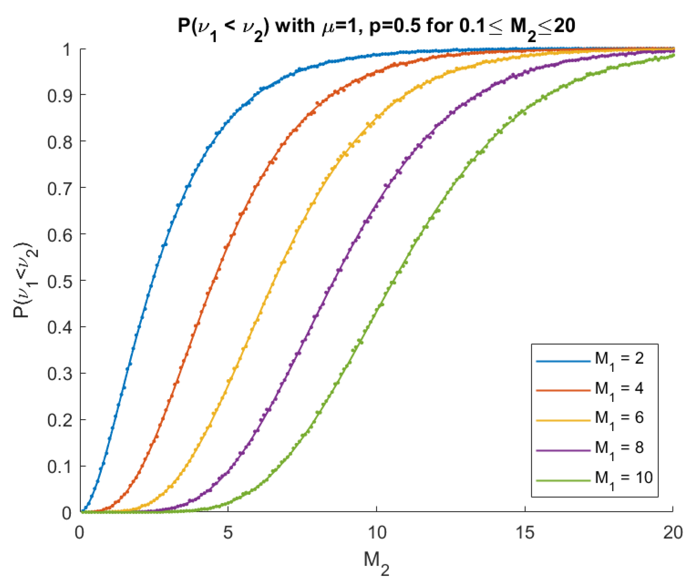
These probabilities are compared to empirical probabilities computed from simulated special case where $\mu =1$, $p=\frac{1}{2}$, and varying values of the thresholds $M_1$ and $M_2$ in the diagrams below.

In Figure 4, predicted results above are plotted as solid curves and empirical probabilities from simulations of 10,000 paths of the process are computed and plotted as dots, which show strong agreement.

We see a sigmoid pattern for the probability ${\nu }_1<{\nu }_2$ when $M_1$ is fixed and $M_2$ grows. If we realize ${\nu }_1<{\nu }_2$ implies $M_1$ is crossed before $M_2$ and that the means of both the node and weight jumps from an attack are equal in this special case, this is very intuitive. A small $M_2$ should be crossed first with high probability resulting in a low probability of the converse, ${\nu }_1<{\nu }_2$. At $M_1=M_2$, the probability is 0.5. A large $M_2$ is rarely crossed first, giving a large probability that ${\nu }_1<{\nu }_2$.

For $P({\nu }_1={\nu }_2)$, we see similarly intuitive results.

Here, in Figure 5 again, simulated and predicted results strongly agree, as does intuition: note that the peak occurs when $M_1=M_2$, which should be when a simultaneous crossing is most common in this case where the mean of the jumps in each dimension is equal.

While we were able to simply compute the probabilities to arbitrary precision with numerical approximations in the example above, this is not always possible, especially at higher dimensions, but the next example demonstrates an alternate path to practical results.

Example 6.

Suppose the jumps of the process ${\mathcal{X}}_i$ are made up of three independent exponential random variables, $\left(X_{i1},X_{i2},X_{i3}\right)$, with parameters ${\mu }_1$, ${\mu }_2$, and ${\mu }_3$, respectively. In a three-dimensional problem, $\mathcal{W}$ is made up of 13 weak orders of four types:

$$\begin{array}{cc}\hfill & {\nu }_1<{\nu }_2<{\nu }_3,{\nu }_1<{\nu }_3<{\nu }_2,{\nu }_2<{\nu }_1<{\nu }_3,{\nu }_2<{\nu }_3<{\nu }_1,{\nu }_3<{\nu }_1<{\nu }_2,{\nu }_3<{\nu }_2<{\nu }_1\hfill \\ & {\nu }_1={\nu }_2<{\nu }_3,{\nu }_1={\nu }_3<{\nu }_2,{\nu }_2={\nu }_3<{\nu }_1\hfill \\ & {\nu }_1<{\nu }_2={\nu }_3,{\nu }_2<{\nu }_1={\nu }_3,{\nu }_3<{\nu }_1={\nu }_2\hfill \\ & {\nu }_1={\nu }_2={\nu }_3\hfill \end{array}$$

Since this example has jumps with independent components, it is enough to compute the four probabilities in the first column and simply apply a permutation to the results and adjust the parameters accordingly to get the others in the same line. We refer the reader to [109] to see the full results, but we reproduce the first one for the sake of discussion. We find

$$\begin{array}{cc}\hfill & P({\nu }_1<{\nu }_2<{\nu }_3)\hfill \\ & =1-e^{-{\mu }_2{M}_2}\left(1+\sqrt{{\mu }_1{\mu }_2{M}_2}{\int }_0^{M_1}\frac{e^{-{\mu }_1\tau }}{\sqrt{\tau }}{I}_1\left(2\sqrt{{\mu }_1{\mu }_2{M}_2\tau }\right)d\tau \right)\hfill \\ & -e^{-{\mu }_3{M}_3}\left(1+\sqrt{{\mu }_2{\mu }_3{M}_3}{\int }_0^{M_2}\frac{e^{-{\mu }_2\tau }}{\sqrt{\tau }}{I}_1\left(2\sqrt{{\mu }_2{\mu }_3{M}_3\tau }\right)d\tau \right)\hfill \\ & +e^{-{\mu }_2{M}_2-{\mu }_3{M}_3}{\mathcal{L}}_{x_1}^{-1}\left(\frac{1}{x_1}{\int }_0^{M_2}\frac{e^{\frac{{\mu }_1{\mu }_2\left(M_2-\tau \right)}{{\mu }_1+x_1}}}{\sqrt{\tau }}{I}_1\left(2\sqrt{\frac{{\mu }_1{\mu }_2{\mu }_3{M}_3\tau }{{\mu }_1+x_1}}\right)d\tau \right)\left(M_1\right)\hfill \end{array}$$

(99)

where $I_1$ is the modified Bessel function of the first kind. The formulas derived for the other 13 probabilities had similar expressions, all made up of a term involving an inverse Laplace transform of an integral involving a Bessel functions and less difficult terms to compute.

The expression above is not quite explicit since some expressions are under integrals and one portion remains under a Laplace transform. The Bessel functions can be computed numerically to high precision quickly and the integrals turn out to be quite easy to approximate to high accuracy with standard numerical integration techniques.

The inverse Laplace transform poses some less widely-understood challenges, but it turns it can reliably be inverted numerically in this instance using the fixed Talbot algorithm [110], which uses trapezoidal numerical integration along a specific deformed contour, using the framework and best practices developed by Abate and Whitt [111].

500 choices of parameters $({\mu }_1,{\mu }_2,{\mu }_3,M_1,M_2,M_3)$ were sampled uniformly fromthe region ${[0.5,3]}^3\times {[10,40]}^3$. For each vector of parameters, 100,000 realizations of the corresponding processes were simulated and empirical probabilities were computed. The numerical scheme for at least one of the 14 probabilities failed to converge properly in 11 of 500 cases, but the maximum error on any of the 14 probabilities in the remaining 489 cases was 0.004, indicating success with numerical inversion.

These two examples demonstrate the result of Theorem 6 is versatile and can be computed explicitly or at least in a form that can be numerically approximated to high precision in numerous interesting special cases.

The probabilities of [109] are unique in this area of study, but what about the full functional ${\Phi }_{\rho }$ in $m+k$ dimensions? This is the focus of some current work by White [112], which has recently confirmed the conjecture made by Dshalalow and Liew [59,60] that their result applies for arbitrarily many active components k for a functional that may be considered in the simplest sense as

$$\begin{array}{c}\hfill {\Phi }_{\rho }={\Phi }_{\rho }\left(u\right)=E{e}^{-u·{\mathcal{A}}_{\rho }},\end{array}$$

(100)

where continuous jumps have a common joint LST $\gamma \left(u\right)=E{e}^{-u·{\mathcal{X}}_1}$. In the spirit of Theorem 6, it has been shown the following holds.

Theorem 7.

If at least one component of $u$has a positive real part, then for each $W\in \mathcal{W}$ where the permutation p is the identity function, then

$$\begin{array}{cc}\hfill {\Phi }_W\left(u\right)& =E{e}^{-u·{\mathcal{A}}_{\rho }}{\mathbf{1}}_W\hfill \\ & ={\mathfrak{H}}_{\chi }\left(\frac{1}{1-\gamma }\sum _{l=0}^{r_1}{(-1)}^l\sum _{\begin{array}{c}J\subset S_j\\ {\parallel J\parallel }_1=l\end{array}}{\gamma }_{{}_{T_2\cup J}}\prod _{j=2}^n\frac{1}{1-{\Gamma }_{T_j}}\sum _{l=0}^{r_j}{(-1)}^l\sum _{\begin{array}{c}J\subset S_j\\ {\parallel J\parallel }_1=l\end{array}}{\Gamma }_{{}_{T_j\cup J}}\right)\hfill \end{array}$$

(101)

where $\gamma =\gamma \left(u+\chi \right)$, ${\gamma }_{{}_B}=\gamma \left(u+{\chi }^B\right)$, and ${\Gamma }_{{}_B}=\gamma \left({\chi }^B\right)$ for $B\subseteq \{1,\dots ,k\}$.

The result readily extends to the situation where p is any permutation, hence giving us an expression for ${\Phi }_W$ for any weak ordering $W\in \mathcal{W}$.

The proof is a somewhat trivial extension to the proof of Theorem 6, but the much larger challenge beyond the work in [112] is to find ${\Phi }_{\rho }$ by summing the ${\Phi }_W$ terms over all weak orderings $W\in \mathcal{W}$,

$$\begin{array}{c}\hfill {\Phi }_{\rho }\left(u\right)=\sum _{W\in \mathcal{W}}{\Phi }_W\left(u\right)\end{array}$$

(102)

Very recently, this problem has been solved in [112] exploiting an interesting recursive pattern in the way in the expressions ${\Phi }_W$ simplify when added together. The result is formulated below.

Theorem 8.

If at least one component of u has a positive real part, then

$$\begin{array}{c}\hfill {\Phi }_{\rho }\left(u\right)=E{e}^{-u·{\mathcal{A}}_{\rho }}={\mathfrak{H}}_{\chi }\left(\frac{\gamma \left(u\right)-\gamma }{1-\gamma }\right).\end{array}$$

(103)

This result has a remarkably simple formula, but an expression analogous to $\frac{\gamma \left(u\right)-\gamma }{1-\gamma }$ is common to many of the other results herein when the pre-exit terms, passive components, and ${\xi }^{\rho }$ terms are omitted from the functional. As such, this theorem most of the time unifies insensitive functionals above, and confirms the conjecture of Dshalalow and Liew [59,60] about a model with k active components.

Of course, many embellishments are possible, such as adding the pre-exit terms, passive components, and ${\xi }^{\rho }$ terms to the functional to seek a fuller functional

$$\begin{array}{cc}\hfill & {\Phi }_{\rho }(\xi ,\alpha ,\varphi ,\beta ,\psi )=E{\xi }^{\rho }{e}^{-\alpha ·{\mathcal{A}}_{\rho -1}}{e}^{i\varphi ·{\mathcal{P}}_{\rho -1}}{e}^{-\beta ·{\mathcal{A}}_{\rho }}{e}^{i\psi ·{\mathcal{P}}_{\rho }}\hfill \end{array}$$

(104)

This is a simple extension of Theorem 8, which will appear in [112]

6. Time Sensitive Analysis of Random Walks

In several models outlined above, particularly those studied by the authors in [65,66] and outlined in Section 3, considered a process running in real time with jumps at times $t_1,t_2,\cdots$, which can only be observed upon an independent delayed renewal process ${\tau }_0$, ${\tau }_1$, ... rather than in real time. In this case, the exit of the process from a k-dimensional rectangular region was studied upon the pre-exit observation time and the post-exit observation time but access to the real exit was unavailable. This approach introduces some insurmountable uncertainty dependent on the crudeness of the observation process ${\left\{{\tau }_n\right\}}_{n=1}^{\infty }$.

A sequence of papers, Dshalalow and his collaborators [50,68,69,73,74,75,76,113] pursue methods referred to as time sensitive analysis that try to offer more precise look into the intermediate time period between the pre-exit observation and post-exit observation times during which the real time exit actually occurs, to glean some further insights about the process upon its exit.

The simplest case of this approach is the study of a one-dimensional discrete random walk by the authors in 2016 [113], where we have a random measure $\mathcal{S}={\sum }_{n=0}^{\infty }{a}_n{\epsilon }_{t_n}$ where $a_n:\Omega \to {\mathbb{Z}}_{+}$ are independent and identically distributed non-negative random variables, and study the continuous-time Poisson process with parameter $\lambda$,

$$\begin{array}{c}\hfill S\left(t\right)=\sum _{n=0}^{\infty }{a}_n{\epsilon }_{t_n}\left([0,t]\right),\end{array}$$

(105)

where each $a_n$ has a common probability-generating function $g\left(z\right)=E{z}^{a_n}$. $S\left(t\right)$ is referred to as the real time stochastic process. The time insensitive methods rely upon study of the process $S\left(t\right)$ through its observed values

$$\begin{array}{c}\hfill S_n=S\left({\tau }_n\right),\end{array}$$

(106)

where the point process ${\tau }_0,{\tau }_1,\dots$ is delayed renewal process representing the observation times of $S\left(t\right).$As a delayed renewal process, the inter-observation times, ${\Delta }_0={\tau }_0$ and ${\Delta }_n={\tau }_n-{\tau }_{n-1},n\in \mathbb{N},$ are independent, and the times for $n\ge 1$ are identically distributed. Denote the Laplace–Stieltjes transforms of each as $L_0\left(\theta \right)=E{e}^{-\theta {\tau }_0}$ and $L\left(\theta \right)=E{e}^{-\theta {\Delta }_1}$, each with Re$\left(\theta \right)\ge 0$.

Then, the increments of the Poisson process between observations satisfy

$$\begin{array}{cc}\hfill & {\gamma }_0\left(z,\theta \right)=E\left[z^{S\left({\tau }_0\right)}{e}^{-\theta {\tau }_0}\right]=L_0\left[\theta +\lambda -\lambda g\left(z\right)\right],\hfill \end{array}$$

(107)

$$\begin{array}{cc}& \gamma \left(z,\theta \right)=E\left[z^{S\left({\Delta }_1\right)}{e}^{-\theta {\Delta }_1}\right]=L\left[\theta +\lambda -\lambda g\left(z\right)\right],\hfill \end{array}$$

(108)

which we assume to be known or readily obtainable.

Given the interval $A=\left[0,M\right],$ where $M\in {\mathbb{Z}}_{+}$, we are interested in the index of the first observed exit of the process from set A, $\nu =$inf$\left\{n\ge 0:S_n\notin A\right\}$. With the one-dimensional time insensitive analysis outlined in Section 2, a functional of the form

$$\begin{array}{c}\hfill {\Phi }_{\nu }(u,v,\vartheta ,\theta )=E{u}^{S_{\nu -1}}{v}^{S_{\nu }}{e}^{-\vartheta t_{\nu -1}-\theta t_{\nu }}\end{array}$$

(109)

was derived. In contrast, one-dimensional time sensitive analysis focuses on targets of the form

$$\begin{array}{cc}\hfill & {\Phi }_{\nu }^1(t,u,v,\vartheta ,\theta ,y)=E{u}^{S_{\nu -1}}{v}^{S_{\nu }}{e}^{-\vartheta {\tau }_{\nu -1}-\theta {\Delta }_{\nu }}{y}^{S\left(t\right)}{\mathbf{1}}_{\{t<{\tau }_{\nu -1}\}},\hfill \end{array}$$

(110)

$$\begin{array}{cc}& {\Phi }_{\nu }^2(t,u,v,\vartheta ,\theta ,y)=E{u}^{S_{\nu -1}}{v}^{S_{\nu }}{e}^{-\vartheta {\tau }_{\nu -1}-\theta {\Delta }_{\nu }}{y}^{S\left(t\right)}{\mathbf{1}}_{\{{\tau }_{\nu -1}\le t<{\tau }_{\nu }\}}\hfill \end{array}$$

(111)

of the value of S upon the observations immediately before and after the real time crossing $S\left({\tau }_{\nu -1}\right)$ and $S\left({\tau }_{\nu }\right)$, the real time value of the process $S\left(t\right)$, and the times of the observations immediately before and after the crossing ${\tau }_{\nu -1}$ and ${\tau }_{\nu }$ themselves. Notice that each functional deals with t placed within a particular random time interval, either before ${\tau }_{\nu -1}$ or between ${\tau }_{\nu -1}$ and ${\tau }_{\nu }$.

In [113], the authors derived formulas for each of these two functionals under a Laplace transform, which are reproduced below.

Theorem 9.

The joint functional ${\Phi }_{\nu }^1(t,u,v,\vartheta ,\theta ,y)$ of the process $S\left(t\right)$ on the interval $[0,{\tau }_{\nu -1})$ satisfies

$$\begin{array}{cc}\hfill {\Phi }_{\nu }^1(t,u,v,\vartheta ,\theta ,y)& ={\mathcal{L}}_x^{-1}\left[{\mathcal{D}}_s^{M-1}\right(\frac{\gamma (v,\theta )-\gamma (vs,\theta )}{x+\lambda g\left(uvs\right)-\lambda g\left(uvys\right)}\hfill \\ & \times \left[\frac{{\gamma }_0(uvs,\vartheta )}{1-\gamma (uvs,\vartheta )}-\frac{{\gamma }_0(uvys,x+\vartheta )}{1-\gamma (uvys,x+\vartheta )}\right]\left)\right]\left(t\right)\hfill \end{array}$$

(112)

Theorem 10.

The joint functional ${\Phi }_{\nu }^2(u,v,\vartheta ,\theta ,y)$ of the process $S\left(t\right)$ on the interval $[{\tau }_{\nu -1},{\tau }_{\nu })$ satisfies

$$\begin{array}{cc}\hfill & {\Phi }_{\nu }^2(t,u,v,\vartheta ,\theta ,y)\hfill \\ & ={\mathcal{L}}_x^{-1}\left[{\mathcal{D}}_s^{M-1}\right(\frac{{\gamma }_0(v,\theta )-{\gamma }_0(vy,x+\theta )}{x+\lambda g\left(v\right)-\lambda g\left(vy\right)}-\frac{{\gamma }_0(vs,\theta )-{\gamma }_0(vys,x+\theta )}{x+\lambda g\left(vs\right)-\lambda g\left(vys\right)}\hfill \\ & +\frac{{\gamma }_0(uvys,x+\theta )}{1-\gamma (uvys,x+\theta )}[\frac{\gamma (v,\theta )-\gamma (vy,x+\theta )}{x+\lambda g\left(v\right)-\lambda g\left(vy\right)}\hfill \\ & -\frac{\gamma (vs,\theta )-\gamma (vys,x+\theta )}{x+\lambda g\left(vs\right)-\lambda g\left(vys\right)}\left]\right)]\left(t\right)\hfill \end{array}$$

(113)

The results are each under a Laplace transform, so it is necessary to evaluate an additional inverse operator to extract probabilistic results from this expression, but they provide a path to some deeper insights than the time sensitive analysis, although they are a bit more of a challenge to derive, as we see in the following example.

Example 7.

To derive practical results, we need merely to specify some details about the real time process and the delayed renewal process of observation times and then apply the transforms. We will make the following assumptions.

• The jump times $\left\{t_1,t_2,\dots \right\}$ form a Poisson point process of rate λ.
• Inter-observation times ${\Delta }_n$ are exponentially distributed with parameter μ, so their LST is $L\left(z\right)=\frac{\mu }{\mu +z}$.
• The marks of the real time process are geometrically distributed with parameter a, so their PGF is $g\left(z\right)=\frac{az}{1-bz}$ where $b=1-a$.
• The initial functional ${\gamma }_0=1$ (i.e., zero initial state and time).

It turns out that in such special cases, time sensitive analysis can be used to derive explicit formulas for joint distributions of random quantities associated with the exit. For example, to find the joint probability mass and distribution function of the exit position of the process and pre-exit observation time, $P\{S_{\nu }=r,{\tau }_{\nu -1}>t\}$, one can find

$$\begin{array}{c}\hfill {\Phi }_{\nu }^1(1,v,0,0,0)=E\left[v^{S_{\nu }}{\mathbf{1}}_{\{t<{\tau }_{\nu -1}\}}\right]\end{array}$$

(114)

explicitly by applying the inverse Laplace transform and $\mathcal{D}$ operator before using properties of probability generating functions to find the function in question as follows.

Proposition 1.

Under Assumptions 1–4,

$$\begin{array}{cc}\hfill & P\{S_{\nu }=r,{\tau }_{\nu -1}>t\}\hfill \\ & =\frac{\mu }{\lambda }\left[R_{0r}+\frac{a\mu }{\mu +\lambda }\sum _{j=1}^{M-1}{R}_{jr}\right]-\frac{\mu }{\lambda +\mu }\left[G_0{R}_{0r}+\sum _{j=1}^{M-1}(G_j-H_{j-1})R_{jr}\right]\hfill \\ & -\frac{\mu }{\lambda }[\sum _{j=0}^{M-1}\sum _{i=0}^{M-1-j}{c}^i{\mathbf{1}}_{\{r=i+j\}}-(b+c)\sum _{j=0}^{M-2}\sum _{i=0}^{M-2-j}{c}^i{\mathbf{1}}_{\{r=i+j+1\}}\hfill \\ & +bc\sum _{j=0}^{M-3}\sum _{i=0}^{M-3-j}{c}^i{\mathbf{1}}_{\{r=i+j+2\}}]\hfill \\ & +\frac{\mu }{\lambda +\mu }[\sum _{j=0}^{M-1}{G}_j\sum _{i=0}^{M-1-j}{c}^i{\mathbf{1}}_{\{r=i+j\}}-\sum _{j=0}^{M-2}(b{G}_j+H_j)\sum _{i=0}^{M-2-j}{c}^i{\mathbf{1}}_{\{r=i+j+1\}}\hfill \\ & +b\sum _{j=0}^{M-3}{H}_j\sum _{i=0}^{M-3-j}{c}^i{\mathbf{1}}_{\{r=i+j+2\}}],\hfill \end{array}$$

(115)

where $c=\frac{b\mu +\lambda }{\mu +\lambda }$,

$$\begin{array}{cc}\hfill & R_{jr}=\left\{\begin{array}{cc}0,\hfill & \mathrm{if}r<j\hfill \\ 1,\hfill & \mathrm{if}r=j\hfill \\ (c-b)c^{r-j-1},\hfill & \mathrm{if}r>j\hfill \end{array}\right.\hfill \end{array}$$

(116)

$$\begin{array}{cc}& G_j=b^j\sum _{k=0}^j\left(\genfrac{}{}{0pt}{}{j}{k}\right){\left(\frac{a}{b}\right)}^k\left[P(k,\lambda t)+\frac{\mu }{\lambda }P(k+1,\lambda t)\right]\hfill \end{array}$$

(117)

$$\begin{array}{cc}& H_j=b^{j+1}\sum _{k=0}^j\left(\genfrac{}{}{0pt}{}{j}{k}\right){\left(\frac{a}{b}\right)}^k\left[P(k,\lambda t)+\left(\frac{\mu }{\lambda }+\frac{a}{b}\right)P(k+1,\lambda t)\right]\hfill \end{array}$$

(118)

and $P(k,\lambda t)=1-\frac{\Gamma (k,\lambda t)}{\Gamma \left(k\right)}$ is the lower regularized gamma function.

While this expression may seem rather large, it is simply a linear combination of terms of the form $G_j$, $H_j$, $R_{jr}$, and some constants associated with the process, which is easy to efficiently compute, as the lower regularized gamma function can be quickly computed to arbitrary precision with common numerical computing tools.

This was just one example of a result that time sensitive analysis permits. It clearly could work for any pair of the time and position random variables upon the exit represented in ${\Phi }_{\nu }^1$ and ${\Phi }_{\nu }^2$, noting in particular,

$$\begin{array}{c}\hfill {\Phi }_{\nu }^1+{\Phi }_{\nu }^2=E\left[u^{S_{\nu -1}}{v}^{S_{\nu }}{e}^{-\vartheta {\tau }_{\nu -1}-\theta {\Delta }_{\nu }}{y}^{S\left(t\right)}{\mathbf{1}}_{\{t<{\tau }_{\nu }\}}\right]\end{array}$$

(119)

allows one to use the post-exit observation ${\tau }_{\nu }$ instead of the pre-exit observation, if preferred.

Some later work by the authors in 2019 [76] pursued time sensitive analysis for a problem extended in several directions: (1) some interesting results are derived for general processes with independent and stationary increments (ISI), (2) instead of one dimension, it assumes a active components and b passive components for a process in ${\mathbb{R}}_{+}^a\times {\mathbb{R}}^b$, and (3) instead of just two times of interest—the pre-exit and post-exit observation previously—the position of the process and time at any finite number of such random times are included in the functional here.

The general results are worth mentioning as they have some interesting implications beyond the scope of this work. Suppose {S$\left(t\right):t\ge 0\}$ is a continuous-time ISI stochastic process, defined on a filtered probability space $\left(\Omega ,\mathcal{F},\left({\mathcal{F}}_t\right),P\right)$. Let $\mathcal{T}=\{T_0,T_1,\dots \}$ be a point process in ${\mathbb{R}}_{+}$ with $T_n=T_{n-1}+{\delta }_n$ where each ${\delta }_n$ is independent of the prior time increments ${\delta }_0,{\delta }_1,\dots ,{\delta }_{n-1}$ and each is non-negative. In this setting, the following interesting result is established regarding the functional

$$\begin{array}{c}\hfill F_n(t,v_0,v_1,\dots ,v_m,y,\mathit{\theta })=E\left[e^{-\sum _{j=0}^m\left(i{v}_j·\mathrm{S}\left(T_j\right)+{\theta }_j{\delta }_j\right)}{e}^{-i\mathit{y}·\mathrm{S}\left(t\right)}{\mathbf{1}}_{[T_{n-1},T_n)}\left(t\right)\right]\end{array}$$

(120)

for each $n=1,\dots ,m$ assuming $v_j,y\in {\mathbb{R}}^{a+b}$ and $\mathit{\theta }=({\theta }_0,\dots ,{\theta }_m)\in {\mathbb{C}}_{+}^{m+1}$, where we denote ${\mathbb{C}}_{+}=\{z\in \mathbb{C}:$Re$\left(z\right)\ge 0\}$. This is a joint characteristic function of the ISI process S$\left(T_j\right)$ at each time in $\mathcal{T}$ with $j\le m$, each corresponding random time increment ${\delta }_n$, and the real time value of the process S$\left(t\right)$, restricted to times in $[T_{n-1},T_n)$.

Denote the Laplace transform of $F_n(t,v_0,v_1,\dots ,v_m,y,\mathit{\theta })$ as

$$\begin{array}{cc}\hfill & F_n^{*}(x,v_0,v_1,\dots ,v_m,y,\mathit{\theta })={\mathcal{L}}_t\left(F_n(t,v_0,v_1,\dots ,v_m,y,\mathit{\theta })\right)\left(x\right).\hfill \end{array}$$

(121)

Theorem 11.

For an independent and stationary increments process $S\left(t\right)$ on the trace σ-algebra $\mathcal{F}\cap \{T_{n-1}\le t\le T_n\}$, where $\mathcal{T}$ is independent of ${\mathcal{F}}_t$, the functional $F_n$ satisfies

$$\begin{array}{cc}\hfill & F_n^{*}(x,v_0,v_1,\dots ,v_m,\mathit{y},\mathit{\theta })\hfill \\ & =\prod _{j=0}^{n-1}{\varphi }_j({\mathit{b}}_j+\mathit{y},{\theta }_j+x)E\left[e^{-{\theta }_n{\delta }_n}\psi ({\mathit{b}}_n+\mathit{y},{\mathit{b}}_n,{\delta }_n,x)\right]\prod _{j=n+1}^m{\varphi }_j({\mathit{b}}_j,{\theta }_j)\hfill \end{array}$$

(122)

under the notation ${\mathit{b}}_j={\Sigma }_{j=0}^m{v}_j$,

$$\begin{array}{cc}\hfill & {\varphi }_j(\mathit{b},\theta )=E\left[e^{-i\mathit{b}·\mathit{S}\left({\delta }_j\right)-\theta {\delta }_j}\right],\hfill \end{array}$$

(123)

$$\begin{array}{cc}& \phi (\mathit{b},t)=E\left[e^{-i\mathit{b}·\mathit{S}\left(t\right)}\right],\hfill \end{array}$$

(124)

$$\begin{array}{cc}& \psi (\mathit{b}+\mathit{y},\mathit{b},r,x)=\left(e^{-x(·)}\phi (\mathit{b}+\mathit{y},·)\right)\ast \phi (\mathit{b},·)\left(r\right).\hfill \end{array}$$

(125)

This result gives a formula for a joint functional on some m independent random times of interest of a very general stochastic process S$\left(t\right)$. If the process is assumed to be a collection of marked Poisson processes, the result simplifies to an interesting result.

Corollary 1.

If $\mathit{S}\left(t\right)$ is made up of $d=a+b$ parallel marked Poisson processes with rates ${\lambda }_1,\dots ,{\lambda }_d$ and $\mathcal{T}$ is independent of ${\mathcal{F}}_t$, then on the trace σ-algebra $\mathcal{F}\cap \{T_{n-1}\le t\le T_n\}$, the functional $F_n$ satisfies

$$\begin{array}{cc}\hfill & F_n^{*}(x,{\mathit{v}}_0,{\mathit{v}}_1,\dots ,{\mathit{v}}_m,\mathit{y},\mathit{\theta })\hfill \\ & =\prod _{j=0}^{n-1}{\varphi }_j(x+{\theta }_j+\mathit{\lambda }·\mathit{G}({\mathit{b}}_j+\mathit{y}))\frac{{\varphi }_n({\theta }_n+\mathit{\lambda }·\mathit{G}\left({\mathit{b}}_n\right))-{\varphi }_n(x+{\theta }_n+\mathit{\lambda }·\mathit{G}({\mathit{b}}_n+\mathit{y}))}{x+\lambda ·(\mathit{G}({\mathit{b}}_n+\mathit{y})-\mathit{G}\left({\mathit{b}}_n\right))}\hfill \\ & \times \prod _{j=n+1}^m{\varphi }_j({\theta }_j+\mathit{\lambda }·\mathit{G}\left({\mathit{b}}_j\right)),\hfill \end{array}$$

(126)

where ${\varphi }_j\left(\theta \right)=E\left[e^{-\theta {\delta }_j}\right]$, $g_j\left(b\right)=E\left[e^{-i\mathrm{b}{X}_{mj}}\right]$, and $\mathit{G}\left(\mathit{b}\right)=\left(1-g_1\left(b_1\right),\dots ,1-g_d\left(b_d\right)\right)$.

Suppose next the process has two active components, $a=2$, and we will make some additional assumptions to turn the process $\mathbf{S}\left(t\right)$ into a random walk and review the related results from [76].

Consider the random measure

$$\begin{array}{c}\hfill \mathcal{S}=\sum _{n=0}^{\infty }\left(a_n^1,a_n^2,{\mathrm{p}}_n\right){\epsilon }_{t_n},\end{array}$$

(127)

where the jumps $\left(a_n^1,a_n^2,{\mathrm{p}}_n\right):\Omega \to {\mathbb{R}}_{+}\times {\mathbb{R}}_{+}\times {\mathbb{R}}^b$ are independent and identically distributed non-negative random vectors, and we study the stochastic process

$$\begin{array}{c}\hfill \mathbf{S}\left(t\right)=\sum _{n=0}^{\infty }\left(a_n^1,a_n^2,{\mathrm{p}}_n\right){\epsilon }_{t_n}\left([0,t]\right),\end{array}$$

(128)

where each jump has a common joint transform $\mathbf{G}\left(z\right)$. The time insensitive methods rely upon study of the process $\mathbf{S}\left(t\right)$ through its observed values

$$\begin{array}{c}\hfill {\mathbf{S}}_n=\mathbf{S}\left({\tau }_n\right)=\sum _{j=0}^n{\mathbf{x}}_j\end{array}$$

(129)

where the point process ${\tau }_0,{\tau }_1,\cdots$ is delayed renewal process representing the observation times of S$\left(t\right)$ with initial LST $L_0\left(\theta \right)=E{e}^{-\theta {\tau }_0}$ and common LST $L\left(\theta \right)=E{e}^{-\theta {\Delta }_1}$ for the inter-observation times. We can represent the joint transforms of ${\mathbf{x}}_n$ as

$$\begin{array}{cc}\hfill & {\gamma }_0(\mathit{v},\vartheta )=E{e}^{-i\mathit{v}·{\mathbf{x}}_0-\vartheta {\tau }_0}\hfill \end{array}$$

(130)

$$\begin{array}{cc}& \gamma (\mathit{v},\vartheta )=E{e}^{-i\mathit{v}·{\mathbf{x}}_1-\vartheta {\Delta }_1}\hfill \end{array}$$

(131)

for $n\ge 1$, which we assume to be known or readily obtainable.

Given the rectangular cylinder $A=\left[0,M_1\right]\times \left[0,M_2\right]\times {\mathbb{R}}^b,$ where $M_1,M_2\in {\mathbb{R}}_{+},$ we are interested in the index of the first observed exit of the process from set A, $\nu =inf\left\{n\ge 0:{\mathit{S}}_n\notin A\right\}$, and we will target the time sensitive functionals

$$\begin{array}{cc}\hfill & {\Phi }_{\nu }^1(t,\mathit{u},\mathit{v},{\theta }_0,\theta ,\mathit{y})=E\left[e^{-i\mathit{u}·{\mathrm{S}}_{\nu -1}-i\mathit{v}·{\mathrm{S}}_{\nu }-{\theta }_0{\tau }_{\nu -1}-\theta {\Delta }_{\nu }-i\mathit{y}·\mathrm{S}\left(t\right)}{\mathit{1}}_{[0,{\tau }_{\nu -1})}\left(t\right)\right]\hfill \end{array}$$

(132)

$$\begin{array}{cc}& {\Phi }_{\nu }^2(t,\mathit{u},\mathit{v},{\theta }_0,\theta ,\mathit{y})=E\left[e^{-i\mathit{u}·{\mathrm{S}}_{\nu -1}-i\mathit{v}·{\mathrm{S}}_{\nu }-{\theta }_0{\tau }_{\nu -1}-\theta {\Delta }_{\nu }-i\mathit{y}·\mathrm{S}\left(t\right)}{\mathit{1}}_{[{\tau }_{\nu -1},{\tau }_{\nu })}\left(t\right)\right]\hfill \end{array}$$

(133)

of the positions of the process upon the pre-exit and post-exit observations, the position at the real time t, and the pre-exit and post-exit times themselves, restricted to the random time intervals $[0,{\tau }_{\nu -1})$ before the pre-passage times and $[{\tau }_{\nu -1},{\tau }_{\nu })$ between the pre-exit and post-exit times.

Through a stochastic summation over a conveniently chosen partition of the sample space, Corollary 1 can be used to derive these functionals in the case where the components of the process are marked Poisson processes.

Theorem 12.

Let $\mathit{S}\left(t\right)$ be the constant interpolation of the process embedded in a process made up of $2+b$ parallel marked Poisson processes of rates ${\lambda }_1,\cdots ,{\lambda }_{2+b}$ where the two active components are discrete, continuous, or mixed. For the process on the trace σ-algebra $\mathcal{F}\cap \{t<{\tau }_{\nu -1}\}$, the joint functional ${\Phi }_{\nu }^1(t,\mathit{u},\mathit{v},{\theta }_0,\theta ,\mathit{y})$ satisfies

$$\begin{array}{cc}\hfill & {\mathcal{L}}_t\left({\Phi }_{\nu }^1(t,\mathit{u},\mathit{v},{\theta }_0,\theta ,\mathit{y})\right)\left(x\right)\hfill \\ & ={\mathfrak{H}}_{\mathit{s}}(\frac{{\gamma }_0(\mathit{u}+\mathit{v}+\mathit{s}+\mathit{y},x+{\theta }_0)}{x+\lambda ·\left(G\right(\mathit{u}+\mathit{v}+\mathit{s})-G(\mathit{u}+\mathit{v}+\mathit{s}+\mathit{y}\left)\right)}\left[\gamma (\mathit{v},\theta )-\gamma (\mathit{v}+\mathit{s},\theta )\right]\hfill \\ & \times \left[\frac{1}{1-\gamma (\mathit{u}+\mathit{v}+\mathit{s},{\theta }_0)}-\frac{1}{1-{\gamma }_0(\mathit{u}+\mathit{v}+\mathit{s}+\mathit{y},x+{\theta }_0)}\right]\hfill \\ & +\frac{{\gamma }_0(\mathit{u}+\mathit{v}+\mathit{s},{\theta }_0)-{\gamma }_0(\mathit{u}+\mathit{v}+\mathit{s}+\mathit{y},x+{\theta }_0)}{x+\lambda ·\left(G\right(\mathit{u}+\mathit{v}+\mathit{s})-G(\mathit{u}+\mathit{v}+\mathit{s}+\mathit{y}\left)\right)}\frac{\gamma (\mathit{v},\theta )-\gamma (\mathit{v}+\mathit{s},\theta )}{1-\gamma (\mathit{u}+\mathit{v}+\mathit{s},{\theta }_0)})\left(\mathit{M}\right).\hfill \end{array}$$

(134)

Theorem 13.

Let $\mathit{S}\left(t\right)$ be the constant interpolation of the process embedded in a process made up of $2+b$ parallel marked Poisson processes of rates ${\lambda }_1,\dots ,{\lambda }_{2+b}$ where the two active components are discrete, continuous, or mixed. For the process on the trace σ-algebra $\mathcal{F}\cap \{{\tau }_{\nu -1}\le t<{\tau }_{\nu }\}$, the joint functional ${\Phi }_{\nu }^2(t,\mathit{u},\mathit{v},{\theta }_0,\theta ,\mathit{y})$ satisfies

$$\begin{array}{cc}\hfill & {\mathcal{L}}_t\left({\Phi }_{\nu }^2(t,\mathit{u},\mathit{v},{\theta }_0,\theta ,\mathit{y})\right)\left(x\right)\hfill \\ & ={\mathcal{G}}_{\mathit{s}}^{-1}(\frac{{\gamma }_0(\mathit{v}+\mathit{y},x+\theta )-{\gamma }_0(\mathit{v},\theta )}{x+\lambda ·\left(G\right(\mathit{v})-G(\mathit{v}+\mathit{y}\left)\right)}-\frac{{\gamma }_0(\mathit{v}+\mathit{s}+\mathit{y},x+\theta )-{\gamma }_0(\mathit{v}+\mathit{s},\theta )}{x+\lambda ·\left(G\right(\mathit{v}+\mathit{s})-G(\mathit{v}+\mathit{s}+\mathit{y}\left)\right)}\hfill \\ & +\frac{{\gamma }_0(\mathit{u}+\mathit{v}+\mathit{s}+\mathit{y},x+{\theta }_0)}{1-\gamma (\mathit{u}+\mathit{v}+\mathit{s}+\mathit{y},x+{\theta }_0)}\hfill \\ & \times [\frac{\gamma (\mathit{v}+\mathit{y},x+\theta )-\gamma (\mathit{v},\theta )}{x+\lambda ·\left(G\right(\mathit{v})-G(\mathit{v}+\mathit{y}\left)\right)}\hfill \\ & -\frac{\gamma (\mathit{v}+\mathit{s}+\mathit{y},x+\theta )-\gamma (\mathit{v}+\mathit{s},\theta )}{x+\lambda ·\left(G\right(\mathit{v}+\mathit{s})-G(\mathit{v}+\mathit{s}+\mathit{y}\left)\right)}\left]\right)\left(\mathit{M}\right).\hfill \end{array}$$

(135)

The expression of Theorem 13 [76] is clearly very similar to the one dimensional time sensitive result from Theorem 10 [113], but this one happens to be for a continuous problem. Indeed, this expression actually is in a similar form to the time insensitive functionals of Theorem 1, Theorem 2 [65], and Theorem 4 [106], a common thread running throughout much of the work discussed in this article.

References

- Pearson, K. The Problem of the Random Walk. Nature 1905, 72, 294. [Google Scholar] [CrossRef]
- Takács, L. On fluctuations of sums of random variables. In Sudies in Probability and Ergodic Theory. Advances in Mathematics. Supplementary Studies; Rota, G.C., Ed.; Academic Press: New York, NY, USA, 1978; Volume 2, pp. 45–93. [Google Scholar]
- Unver, I.; Tundzh, Y.S.; Ibaev, E. Laplace-Stieltjes transform of the distribution of the first moment of crossing the level a (a > 0) by a semi-Markovian random walk with positive drift and negative jumps. Autom. Control. Comput. Sci. 2014, 48, 144–149. [Google Scholar] [CrossRef]
- Andersen, E.S. On the fluctuations of sums of random variables. Math. Scand. 1953, 1, 263. [Google Scholar] [CrossRef] [Green Version]
- Andersen, E.S. On the fluctuations of sums of random variables II. Math. Scand. 1954, 2, 194. [Google Scholar] [CrossRef] [Green Version]
- Rayleigh, J.W.S. The Problem of the Random Walk. Nature 1905, 72, 318. [Google Scholar] [CrossRef] [Green Version]
- Takács, L. Random walk on a finite group. Acta Sci. Math. 1983, 45, 395–408. [Google Scholar]
- Takacs, C. Biased random walks on directed trees. Probab. Theory Relat. Fields 1983, 111, 123–139. [Google Scholar] [CrossRef]
- Dshalalow, J.H.; Syski, R. Lajos Takács and his work. J. Appl. Math. Stoch. Anal. 1994, 7, 215–237. [Google Scholar] [CrossRef] [Green Version]
- Van den Berg, M. Exit and Return of a Simple Random Walk. Potential Anal. 2005, 23, 45–53. [Google Scholar] [CrossRef]
- Mogul’skiĭ, A.A. Local limit theorem for the first crossing time of a fixed level by a random walk. Sib. Adv. Math. 2010, 20, 191–200. [Google Scholar] [CrossRef]
- Becker, M.; König, W. Moments and Distribution of the Local Times of a Transient Random Walk on ℤd. J. Theor. Probab. 2008. [Google Scholar] [CrossRef]
- Csáki, E.; Földes, A.; Révész, P. Maximal Local Time of a d-dimensional Simple Random Walk on Subsets. J. Theor. Probab. 2005, 18, 687–717. [Google Scholar] [CrossRef] [Green Version]
- Gluck, D. First hitting times for some random walks on finite groups. J. Theor. Probab. 1999, 12, 739–755. [Google Scholar] [CrossRef]
- Fayolle, G.; Iasnogorodski, R.; Malyshev, V. Random Walks in the Quarter Plane; Springer: Berlin/Heisenberg, Germany, 2017. [Google Scholar] [CrossRef]
- Hildebrand, M. A survey of results on random random walks on finite groups. Probab. Surv. 2005, 2. [Google Scholar] [CrossRef]
- Montroll, E.W.; Weiss, G.H. Random Walks on Lattices. II. J. Math. Phys. 1965, 6, 167–181. [Google Scholar] [CrossRef]
- Kutner, R.; Masoliver, J. The continuous time random walk, still trendy: Fifty-year history, state of art and outlook. Eur. Phys. J. B 2017, 90. [Google Scholar] [CrossRef] [Green Version]
- Scalas, E. The application of continuous-time random walks in finance and economics. Phys. A Stat. Mech. Its Appl. 2006, 362, 225–239. [Google Scholar] [CrossRef]
- Balakrishnan, V.; Khantha, M. First passage time and escape time distributions for continuous time random walks. Pramana 1983, 21, 187–200. [Google Scholar] [CrossRef]
- Blanchard, P.; Volchenkov, D. Random Walks and Diffusions on Graphs and Databases; Springer: Berlin/Heisenberg, Germany, 2011. [Google Scholar] [CrossRef] [Green Version]
- Brémaud, P. Discrete Probability Models and Methods; Springer: Berlin/Heisenberg, Germany, 2017. [Google Scholar] [CrossRef]
- Fujie, F.; Zhang, P. Covering Walks in Graphs; Springer: New York, NY, USA, 2014. [Google Scholar] [CrossRef]
- Sarkar, P.; Moore, A.W. Random Walks in Social Networks and their Applications: A Survey. In Social Network Data Analytics; Springer: New York, NY, USA, 2011; Chapter 3. [Google Scholar] [CrossRef]
- Shi, Z. Branching Random Walks; Springer: Berlin/Heisenberg, Germany, 2015. [Google Scholar] [CrossRef]
- Telcs, A. Random Walks on graphs, electric networks and fractals. Probab. Theory Relat. Fields 1989, 82, 435–449. [Google Scholar] [CrossRef]
- Abolnikov, L.; Dshalalow, J.H. Ergodicity conditions and invariant probability measure for an embedded Markov chain in a controlled bulk queueing system with a bilevel service delay discipline part I. Appl. Math. Lett. 1992, 5, 25–27. [Google Scholar] [CrossRef] [Green Version]
- Abolnikov, L.; Dshalalow, J.H. A first passage problem and its applications to the analysis of a class of stochastic models. J. Appl. Math. Stoch. Anal. 1992, 5, 83–97. [Google Scholar] [CrossRef] [Green Version]
- Abolnikov, L.; Dshalalow, J.H. On a multilevel controlled bulk queueing system MX/Gr,R/1. J. Appl. Math. Stoch. Anal. 1992, 5, 237–260. [Google Scholar] [CrossRef] [Green Version]
- Abolnikov, L.M.; Dshalalow, J.H. Semi-regenerative analysis of controlled bulk queueing systems with a bilevel service delay discipline and some ergodic theorems. Comput. Math. Appl. 1993, 25, 107–116. [Google Scholar] [CrossRef] [Green Version]
- Abolnikov, L.; Agarwal, R.P.; Dshalalow, J.H. Random walk analysis of parallel queueing stations. Math. Comput. Model. 2008, 47, 452–468. [Google Scholar] [CrossRef]
- Abolnikov, L.M.; Dshalalow, J.H.; Dukhovny, A.M. On stochastic processes in a multilevel control bulk queueing system. Stoch. Anal. Appl. 1992, 10, 155–179. [Google Scholar] [CrossRef]
- Abolnikov, L.M.; Dshalalow, J.H.; Dukhovny, A.M. Stochastic analysis of a controlled bulk queueing system with continuously operating server: Continuous time parameter queueing process. Stat. Probab. Lett. 1993, 16, 121–128. [Google Scholar] [CrossRef]
- Abolnikov, L.M.; Dshalalow, J.H.; Dukhovny, A.M. A multilevel control bulk queueing system with vacationing server. Oper. Res. Lett. 1993, 13, 183–188. [Google Scholar] [CrossRef]
- Dshalalow, J.H. On a first passage problem in general queueing systems with multiple vacations. J. Appl. Math. Stoch. Anal. 1992, 5, 177–192. [Google Scholar] [CrossRef]
- Dshalalow, J.H.; Tadj, L. On applications of first excess level random processes to queueing systems with random server capacity and capacity dependent service time. Stochastics Stoch. Rep. 1993, 45, 45–60. [Google Scholar] [CrossRef]
- Dshalalow, J.H. First excess levels of vector processes. J. Appl. Math. Stoch. Anal. 1994, 7, 457–464. [Google Scholar] [CrossRef] [Green Version]
- Dshalalow, J. First excess level analysis of random processes in a class of stochastic servicing systems with global control. Stoch. Anal. Appl. 1994, 12, 75–101. [Google Scholar] [CrossRef]
- Dshalalow, J. Excess level processes in queueing. In Advances in Queueing; Dshalalow, J., Ed.; CRC Press: Boca Raton, FL, USA, 1995; pp. 243–262. [Google Scholar]
- Dshalalow, J. On the level crossing of multi-dimensional delayed renewal processes. J. Appl. Math. Stoch. Anal. 1997, 10, 355–361. [Google Scholar] [CrossRef] [Green Version]
- Dshalalow, J.H.; Motir, R. Random Walk Processes in a Bilevel (M-N)-Policy Queue with Multiple Vacations. Qual. Technol. Quant. Manag. 2011, 8, 303–332. [Google Scholar] [CrossRef]
- Dshalalow, J.H.; Russell, G. On a single-server queue with fixed accumulation level, state dependent service, and semi-Markov modulated input flow. Int. J. Math. Math. Sci. 1992, 15, 593–600. [Google Scholar] [CrossRef] [Green Version]
- Dshalalow, J.H.; Yellen, J. Bulk input queues with quorum and multiple vacations. Math. Probl. Eng. 1996, 2, 95–106. [Google Scholar] [CrossRef]
- Agarwal, R.; Dshalalow, J. New fluctuation analysis of D-policy bulk queues with multiple vacations. Math. Comput. Model. 2005, 41, 253–269. [Google Scholar] [CrossRef]
- Abolnikov, L.; Dshalalow, J.H.; Treerattrakoon, A. On a dual hybrid queueing system. Nonlinear Anal. Hybrid Syst. 2008, 2, 96–109. [Google Scholar] [CrossRef]
- Dshalalow, J.H. Queues with hysteretic control by vacation and post-vacation periods. Queueing Syst. 1998, 29, 231–268. [Google Scholar] [CrossRef]
- Dshalalow, J.; Dikong, E. On generalized hysteretic control queues with modulated input and state dependent service. Stoch. Anal. Appl. 1999, 17, 937–961. [Google Scholar] [CrossRef]
- Dikong, E.E.; Dshalalow, J.H. Bulk input queues with hysteretic control. Queueing Syst. 1999, 32, 287–304. [Google Scholar] [CrossRef]
- Dshalalow, J.; Kim, S.; Tadj, L. Hybrid queueing systems with hysteretic bilevel control policies. Nonlinear Anal. Theory Methods Appl. 2006, 65, 2153–2168. [Google Scholar] [CrossRef]
- Bacot, J.B.; Dshalalow, J. A bulk input queueing system with batch gated service and multiple vacation policy. Math. Comput. Model. 2001, 34, 873–886. [Google Scholar] [CrossRef]
- Dshalalow, J.H.; Merie, A. Fluctuation analysis in queues with several operational modes and priority customers. Top 2018, 26, 309–333. [Google Scholar] [CrossRef]
- Dshalalow, J.H.; Merie, A.; White, R.T. Fluctuation Analysis in Parallel Queues with Hysteretic Control. Methodol. Comput. Appl. Probab. 2019, 22, 295–327. [Google Scholar] [CrossRef]
- Dshalalow, J.H.; Huang, W. A stochastic games with a two-phase conflict. In Jubilee Volume: Legacy of the Legend, Professor V. Lakshmikantham; Cambridge Scientific Publishers: Cottenham, UK, 2009; pp. 201–209. [Google Scholar]
- Dshalalow, J.H.; Huang, W. Tandem antagonistic games. Nonlinear Anal. Ser. Theory Methods 2009, 71, 259–270. [Google Scholar]
- Dshalalow, J.H.; Huang, W. Sequential antagonistic games with an auxiliary initial phase. In Functional Equations, Difference Inequalities, and Ulam Stability Notions (F.U.N.); Nova Science Publishers: New York, NY, USA, 2010; Chapter 2; pp. 15–36. [Google Scholar]
- Dshalalow, J.H. Fluctuations of Recurrent Processes and Their Applications to the Stock Market. Stoch. Anal. Appl. 2004, 22, 67–79. [Google Scholar] [CrossRef]
- Dshalalow, J.H. On exit times of a multivariate random walk with some applications to finance. Nonlinear Anal. 2005, 63, 569–577. [Google Scholar] [CrossRef]
- Dshalalow, J.H.; Liew, A. Level crossings of an oscillating marked random walk. Comput. Math. Appl. 2006, 52, 917–932. [Google Scholar] [CrossRef] [Green Version]
- Dshalalow, J.; Liew, A. On fluctuations of a multivariate random walk with some applications to stock options trading and hedging. Math. Comput. Model. 2006, 44, 931–944. [Google Scholar] [CrossRef]
- Dshalalow, J.H.; Liew, A. On exit times of a multivariate random walk and its embedding in a quasi Poisson process. Stoch. Anal. Appl. 2006, 24, 451–474. [Google Scholar] [CrossRef]
- Dshalalow, J.H.; Iwezulu, K. Discrete versus continuous operational calculus in antagonistic stochastic games. São Paulo J. Math. Sci. 2017, 11, 471–489. [Google Scholar] [CrossRef]
- Dshalalow, J.H.; Ke, H.J. Layers of noncooperative games. Nonlinear Anal. Ser. Theory Methods 2009, 71, 283–291. [Google Scholar] [CrossRef]
- Dshalalow, J.H.; Ke, H.J. Multilayers in a modulated stochastic game. J. Math. Anal. Appl. 2009, 353, 553–565. [Google Scholar] [CrossRef] [Green Version]
- Dshalalow, J.H.; Treerattrakoon, A. Set-theoretic inequalities in stochastic noncooperative games with coalition. J. Inequalities Appl. 2008, 2008, 1–14. [Google Scholar] [CrossRef]
- Dshalalow, J.H.; White, R. On Reliability of Stochastic Networks. Neural Parallel Sci. Comput. 2013, 21, 141–160. [Google Scholar]
- Dshalalow, J.H.; White, R. On Strategic Defense in Stochastic Networks. Stoch. Anal. Appl. 2014, 32, 365–396. [Google Scholar] [CrossRef]
- Dshalalow, J.H. Time dependent analysis of multivariate marked renewal processes. J. Appl. Probab. 2001, 38, 707–721. [Google Scholar] [CrossRef]
- Agarwal, R.P.; Dshalalow, J.H.; O’Regan, D. Time sensitive functionals of marked Cox processes. J. Math. Anal. Appl. 2004, 293, 14–27. [Google Scholar] [CrossRef] [Green Version]
- Al-Matar, N.; Dshalalow, J.H. Time sensitive functionals in a queue with sequential maintenance. Stoch. Model. 2011, 27, 687–704. [Google Scholar] [CrossRef]
- Dshalalow, J.H. Random Walk Analysis in Antagonistic Stochastic Games. Stoch. Anal. Appl. 2008, 26, 738–783. [Google Scholar] [CrossRef]
- Dshalalow, J.H. On multivariate antagonistic marked point processes. Math. Comput. Model. 2009, 49, 432–452. [Google Scholar] [CrossRef]
- Dshalalow, J.H.; Bacot, J.B. On functionals of a marked Poisson process observed by a renewal process. Int. J. Math. Math. Sci. 2001, 26, 427–436. [Google Scholar] [CrossRef] [Green Version]
- Dshalalow, J.H.; Nandyose, K.M. Continous time interpolation of monotone marked random measures with applications. Neural Parallel Sci. Comput. 2018, 26, 119–141. [Google Scholar] [CrossRef]
- Dshalalow, J.H.; Nandyose, K.M. Real time analysis of signed marked random measures with applications to finance and insurance. Nonlinear Dyn. Syst. Theory 2018, 19, 36–54. [Google Scholar]
- Dshalalow, J.H.; Nandyose, K.M.; White, R.T. Time dependent analysis of stochastic games of three players with applications. Math. Stat. 2021. pending minor revision. [Google Scholar]
- White, R.T.; Dshalalow, J.H. Characterizations of random walks on random lattices and their ramifications. Stoch. Anal. Appl. 2019, 38, 307–342. [Google Scholar] [CrossRef]
- Antal, T.; Redner, S. Escape of a Uniform Random Walk from an Interval. J. Stat. Phys. 2006, 123, 1129–1144. [Google Scholar] [CrossRef] [Green Version]
- Hughes, B.D. Random Walks and Random Environments; Clarendon Press Oxford University Press: Oxford, NY, USA, 1995. [Google Scholar]
- Redner, S. A Guide to First-Passage Processes; Cambridge University Press: Cambridge, UK, 2001. [Google Scholar] [CrossRef]
- Kyprianou, A.E.; Pistorius, M.R. Perpetual options and Canadization through fluctuation theory. Ann. Appl. Probab. 2003, 13, 1077–1098. [Google Scholar] [CrossRef] [Green Version]
- Muzy, J.; Delour, J.; Bacry, E. Modelling fluctuations of financial time series: From cascade process to stochastic volatility model. Eur. Phys. J. B 2000, 17, 537–548. [Google Scholar] [CrossRef] [Green Version]
- Uchaikin, V.V.; Gusarov, G.G. Analysis of the structure function for the spatial distribution of galaxies in the random-walk model. Russ. Phys. J. 1997, 40, 707–710. [Google Scholar] [CrossRef]
- Zhou, J.L.; Sun, Y.S.; Zhou, L.Y. Evidence for Lévy Random Walks in the Evolution of Comets from the Oort Cloud. Celest. Mech. Dyn. Astron. 2002, 84, 409–427. [Google Scholar] [CrossRef]
- Odagaki, T.; Kasuya, K. Alzheimer random walk. Eur. Phys. J. B 2017, 90. [Google Scholar] [CrossRef]
- Jabbari, B.; Zhou, Y.; Hillier, F.S. A decomposable random walk model for mobility in wireless communications. Telecommun. Syst. 2001, 16, 523–537. [Google Scholar] [CrossRef]
- Asmussen, S. Phase-Type Representations in Random Walk and Queueing Problems. Ann. Probab. 1992, 20, 772–789. [Google Scholar] [CrossRef]
- Bayer, N.; Boxma, O.J. Wiener-Hopf analysis of an M/G/1 queue with negative customers and of a related class of random walks. Queueing Syst. 1996, 23, 301–316. [Google Scholar] [CrossRef] [Green Version]
- Cohen, J. Random Walk with a Heavy-Tailed Jump Distribution. Queueing Syst. 2002, 40, 35–73. [Google Scholar] [CrossRef]
- Gannon, M.; Pechersky, E.; Suhov, Y.; Yambartsev, A. Random walks in a queueing network environment. J. Appl. Probab. 2016, 53, 448–462. [Google Scholar] [CrossRef] [Green Version]
- Guillemin, F.; van Leeuwaarden, J.S.H. Rare event asymptotics for a random walk in the quarter plane. Queueing Syst. 2010, 67, 1–32. [Google Scholar] [CrossRef] [Green Version]
- Janssen, A.; van Leeuwaarden, J. Spitzer’s identity for discrete random walks. Oper. Res. Lett. 2018, 46, 168–172. [Google Scholar] [CrossRef] [Green Version]
- Lemoine, A.J. On Random Walks and StableGI/G/1 Queues. Math. Oper. Res. 1976, 1, 159–164. [Google Scholar] [CrossRef]
- Stadje, W. The embedded random walk in the stationary M/M/1 queue. Methodol. Comput. Appl. Probab. 2002, 4, 143–151. [Google Scholar] [CrossRef]
- Zorine, A.V. Study of a Service Process by a Loop Algorithm by Means of a Stopped Random Walk. In Information Technologies and Mathematical Modelling. Queueing Theory and Applications; Springer: Berlin/Heisenberg, Germany, 2019; pp. 121–135. [Google Scholar] [CrossRef]
- Bingham, N.H. Fluctuation theory in continuous time. Adv. Appl. Probab. 1975, 7, 705–766. [Google Scholar] [CrossRef]
- Bingham, N.H. Random walk and fluctuation theory. In Handbook of Statistics; Shanbhag, D.N., Rao, C.R., Eds.; Elsevier: Amsterdam, The Netherlands, 2001; Volume 19, pp. 171–213. [Google Scholar]
- Bladt, M.; Nielsen, B.F. Matrix-Exponential Distributions in Applied Probability; Springer: New York, NY, USA, 2017. [Google Scholar] [CrossRef]
- Foss, S.; Korshunov, D.; Zachary, S. An Introduction to Heavy-Tailed and Subexponential Distributions; Springer: New York, NY, USA, 2013. [Google Scholar] [CrossRef]
- Gut, A. Stopped Random Walks; Springer: New York, NY, USA, 2009. [Google Scholar] [CrossRef]
- Iksanov, A. Renewal Theory for Perturbed Random Walks and Similar Processes; Springer: Berlin/Heisenberg, Germany, 2016. [Google Scholar] [CrossRef]
- Lawler, G.F. Intersections of Random Walks; Springer: New York, NY, USA, 2013. [Google Scholar] [CrossRef]
- Slade, G. The Lace Expansion and Its Applications; Springer: Berlin/Heisenberg, Germany, 2006. [Google Scholar] [CrossRef] [Green Version]
- Telcs, A. The Art of Random Walks; Springer: Berlin/Heisenberg, Germany, 2006. [Google Scholar] [CrossRef]
- Wijesundera, I.; Halgamuge, M.N.; Nanayakkara, T.; Nirmalathas, T. Natural Disasters, When Will They Reach Me? Springer: Singapore, 2016. [Google Scholar] [CrossRef]
- Dshalalow, J.H. Single-server queues with controlled bulk service, random accumulation level, and modulated input. Stoch. Anal. Appl. 1993, 11, 29–41. [Google Scholar] [CrossRef]
- White, R.T. Reliability of networks under stochastic attacks. manuscript in progress.
- Agarwal, R.P.; Dshalalow, J.H.; O’Regan, D. Random observations of marked Cox processes. Time insensitive functionals. J. Math. Anal. Appl. 2004, 293, 1–13. [Google Scholar] [CrossRef] [Green Version]
- Agarwal, R.P.; Dshalalow, J.H. On multivariate delayed recurrent processes. Pan Am. Math. J. 2005, 15, 35–49. [Google Scholar]
- White, R.T. On the exiting patterns of sums of independent random vectors with an application to stochastic networks. 2021. submitted. [Google Scholar]
- Talbot, A. The Accurate Numerical Inversion of Laplace Transforms. IMA J. Appl. Math. 1979, 23, 97–120. [Google Scholar] [CrossRef]
- Abate, J.; Whitt, W. A Unified Framework for Numerically Inverting Laplace Transforms. Informs J. Comput. 2006, 18, 408–421. [Google Scholar] [CrossRef]
- White, R.T. On exits and overshoots of dependent jump processes. manuscript in progress.
- Dshalalow, J.H.; White, R.T. Time sensitive analysis of independent and stationary increment processes. J. Math. Anal. Appl. 2016, 443, 817–833. [Google Scholar] [CrossRef] [Green Version]
Figure 1.
The process confined to .
Figure 2.
Predicted and empirical (simulated) probabilities for parameters .
Figure 3.
Figure 4.
Predicted and empirical (simulated) probabilities with parameters , , and for various values.
Figure 5.
Publisher’s Note: MDPI stays neutral with regard to jurisdictional claims in published maps and institutional affiliations. |
© 2021 by the authors. Licensee MDPI, Basel, Switzerland. This article is an open access article distributed under the terms and conditions of the Creative Commons Attribution (CC BY) license (https://creativecommons.org/licenses/by/4.0/).
Share and Cite
MDPI and ACS Style
Dshalalow, J.H.; White, R.T. Current Trends in Random Walks on Random Lattices. Mathematics 2021, 9, 1148. https://doi.org/10.3390/math9101148
AMA Style
Dshalalow JH, White RT. Current Trends in Random Walks on Random Lattices. Mathematics. 2021; 9(10):1148. https://doi.org/10.3390/math9101148
Chicago/Turabian StyleDshalalow, Jewgeni H., and Ryan T. White. 2021. "Current Trends in Random Walks on Random Lattices" Mathematics 9, no. 10: 1148. https://doi.org/10.3390/math9101148
Note that from the first issue of 2016, this journal uses article numbers instead of page numbers. See further details here.