Article

The Curve Estimation of Combined Truncated Spline and Fourier Series Estimators for Multiresponse Nonparametric Regression

by
Helida Nurcahayani
1,2,
I Nyoman Budiantara
1,* and
Ismaini Zain
1
1
Department of Statistics, Faculty of Science and Data Analytics, Institut Teknologi Sepuluh Nopember, Surabaya 60111, Indonesia
2
BPS—Statistics of Daerah Istimewa Yogyakarta Province, Bantul 55183, Indonesia
*
Author to whom correspondence should be addressed.
Mathematics 2021, 9(10), 1141; https://doi.org/10.3390/math9101141
Submission received: 11 April 2021 / Revised: 14 May 2021 / Accepted: 17 May 2021 / Published: 18 May 2021
(This article belongs to the Section Probability and Statistics)

Abstract

:
Nonparametric regression becomes a potential solution if the parametric regression assumption is too restrictive while the regression curve is assumed to be known. In multivariable nonparametric regression, the pattern of each predictor variable’s relationship with the response variable is not always the same; thus, a combined estimator is recommended. In addition, regression modeling sometimes involves more than one response, i.e., multiresponse situations. Therefore, we propose a new estimation method of performing multiresponse nonparametric regression with a combined estimator. The objective is to estimate the regression curve using combined truncated spline and Fourier series estimators for multiresponse nonparametric regression. The regression curve estimation of the proposed model is obtained via two-stage estimation: (1) penalized weighted least square and (2) weighted least square. Simulation data with sample size variation and different error variance were applied, where the best model satisfied the result through a large sample with small variance. Additionally, the application of the regression curve estimation to a real dataset of human development index indicators in East Java Province, Indonesia, showed that the proposed model had better performance than uncombined estimators. Moreover, an adequate coefficient of determination of the best model indicated that the proposed model successfully explained the data variation.

1. Introduction

As one of the renowned methods of regression analysis, parametric regression has been used for many years in various scientific fields. However, some parametric regression assumptions are too restrictive, such as identifying a regression curve’s shape with some prespecified functional form (e.g., linear, quadratic, or cubic) [1]. In real datasets, not all regression curves have a visible pattern due to the absence of relationship information between response and predictor variables. Therefore, in such scenarios, nonparametric regression analysis is more recommended [2]. Nonparametric regression is able to degrade the misspecification risk because data inherently represent the real shape of a regression curve without interference due to the researcher’s subjectivity [2].
To date, researchers have investigated various functions for estimating the regression curve in nonparametric regression, such as spline [3,4,5,6], Fourier series [7,8,9], kernel [10,11,12], polynomial [13,14,15], and wavelet [16,17,18] functions. The present study explores the nonparametric regression approach to analyzing spatial data, i.e., the use of the nonparametric truncated spline function in geographically weighted regression [19,20]. In nonparametric regression with more than one predictor variable (multivariable), the pattern of the relationship between each predictor variable and the response variable is not always the same; therefore, in this study, we employ a nonparametric regression model with a combined estimator. Considering the concept of semiparametric regression, some studies have proposed combined estimator models to estimate the regression curve, such as spline and kernel functions [21,22,23]. Similarly, in [24], the researchers developed a combined estimator of kernel and Fourier series, whereas in [25,26,27], the researchers presented nonparametric regression with a mixed estimator of truncated spline and Fourier series. Recently, researchers have also been giving attention to a mixed model of longitudinal data, as carried out by [28].
So far, studies on nonparametric regression with combined estimators have not dealt with more than two responses, i.e., multiresponse nonparametric regression. Numerous studies on nonparametric regression have been applied to many scientific fields, such as sociodemographic analysis [23,24,25,26], finance [5,29], climatology [4], and economics [30], wherein some cases have involved real data with two or more correlated response variables. Therefore, this study makes a major contribution to the research on multiresponse nonparametric regression by using a combined estimator. Of the several types of regression functions for nonparametric regression, the truncated spline function has the major advantages of high flexibility, good visual interpretation, and the ability to handle smooth function characters and data that have changed behavior at certain subintervals [2]. On the other hand, the Fourier series function is used to estimate the regression curve if the data are smooth and follow a repeated pattern at specific intervals [9]. The Fourier series function is also a trigonometric polynomial that can adjust the data’s local nature effectively. In this study, we adopt a cosine Fourier series function [9], which follows a trend line as the regression curve estimator. A Fourier series with a cosine function was employed since it is an even function, such that the second derivative usually mathematically obtains a scalar or a nonzero value. Furthermore, the penalties in the penalized least square method can be well defined. Considering some of the advantages of these two functions, as outlined above, this study highlights the combined use of truncated spline and Fourier series estimators for multiresponse nonparametric regression.
One of the most well-known tools for the estimation of regression is the ordinary least square (OLS) method. However, the OLS method cannot be directly used in nonparametric regression because of the unknown curve shape. By utilizing smooth, continuous, and differentiable properties, as well as other components, the OLS method was modified with conditional optimization to create the penalized least-square (PLS) regression method [31]. The combined use of estimators for multiresponse nonparametric regression leads to the use of an error variance–covariance matrix as a weighting matrix. Therefore, PLS optimization is still added with a weight; accordingly, the proposed model was obtained through penalized weighted least square (PWLS) optimization. To evaluate the proposed model performance, we employed a simulation study with three different sample sizes and three error variances and applied the proposed model to a real dataset.
Given the view above, the objective of this study is to obtain a curve estimation using combined truncated spline and Fourier series estimators for multiresponse nonparametric regression. This aim is followed by estimating an error variance–covariance matrix as a weighting matrix. To estimate the proposed model, a two-stage estimation method was used. Stage 1 was to estimate the Fourier series component using PWLS optimization. The following stage was to estimate the truncated spline component by utilizing weighted least square (WLS) optimization. In addition to curve estimation, we attempted to simulate and apply the proposed model to a dataset of the HDI in East Java Province, Indonesia. The paper is organized as follows: Section 1 provides an overview of the topic while identifying the knowledge gap and stating the aims of the research. Section 2 describes the truncated spline function and the Fourier series function, along with the PWLS method. Section 3 presents the findings of the regression curve estimation via the combined use of truncated spline and Fourier series estimators for multiresponse nonparametric regression, along with an estimation of the variance–covariance matrix, smoothing parameter selection, and a simulation study following the application of a real dataset. Section 4 gives a brief conclusion and makes future recommendations.

2. Materials and Methods

2.1. Multiresponse Nonparametric Regression, Truncated Spline Function, and Fourier Series Function

Given paired data ( y 1 i , y 2 i , , y r i x 1 i , x 2 i , , x p i , z 1 i , z 2 i , , z q i ) , the relationship between response ( y 1 i , y 2 i , , y r i )   and predictor ( x 1 i , x 2 i , , x p i , z 1 i , z 2 i , , z q i ) variables is assumed to follow multiresponse nonparametric regression, as follows:
y h i = μ h i ( x 1 i , x 2 i , , x p i , z 1 i , z 2 i , , z q i ) + ε h i , ε h i ~ N ( 0 , σ h 2 )
where h = 1 , 2 , , r and i = 1 , 2 , , n . In this study, r is defined as the number of response variables, and n refers to the number of observations for each response and predictor variable. For convenience, Equation (1) can be rewritten in the following matrix form:
y = μ ( x , z ) + ε
The regression curve in Equation (1) can be assumed to be an additive model.
μ h i ( x 1 i , x 2 i , , x p i , z 1 i , z 2 i , , z q i ) = j = 1 p f h j ( x j i ) + k = 1 q g h k ( z k i ) .
In Equation (3), the regression curve f h j ( x j i ) ; j = 1 ,   2 ,   ,   p is assumed to be smooth and is approached by a truncated spline function. Meanwhile, the regression curve g h k ( z k i ) ; k = 1 , 2 , , q is approached by a Fourier series function, which assumes that the regression curve is unknown and is contained in continuous space C [ 0 , π ] . Hence, the multiresponse nonparametric regression in Equation (3) can be written as
y h i = j = 1 p f h j ( x j i ) + k = 1 q g h k ( z k i ) + ε h i ,   ε h i ~ N ( 0 , σ h 2 ) .
Under the assumption ε h i ~ N ( 0 , σ h 2 ) , as described in [32], c o r r ( ε h i ε i ) = ρ for h ;   h , = 1 , 2 , , r . This term refers to situations in which the response variables y h i and y i are a pair, such that a correlation between the h -th response and the -th response yields c o r r ( ε h i ε i ) = ρ , and zero otherwise. The error correlation between responses is the same for every response, defined as ρ = cov ( ε h i ε i ) σ h h σ ; i = 1 , 2 , , n ; h ;   h , = 1 , 2 , , r .
Thus, the regression curve f h j ( x j i ) in Equation (4) is approached by a linear truncated spline function with knots K h j 1 ,   K h j 2 , , K h j u , as follows:
f h j ( x j i ) = α h j x j i + s = 1 u β h j s ( x j i K h j s ) + ,
with the truncated function
( x j i K h j s ) + = { ( x j i K h j s ) + , x j i K h j s 0 , x j i < K h j s
Adopting the Fourier series function in [9], g h k ( z k i ) in Equation (4) is approached by a Fourier series cosine function following the trend line ( b h k z k i ), as given in Equation (6):
g h k ( z k i ) = b h k z k i + 1 2 a o h k + t = 1 T a t h k cos t z k i .

2.2. Penalized Weighted Least Square

Suppose that the dataset ( y 1 i , y 2 i , , y r i , x 1 i , x 2 i , , x p i , z 1 i , z 2 i , , z q i ) follows the multiresponse nonparametric regression in Equation (1) and is rewritten in matrix form as Equation (2). The random error ε in Equation (2) is normally distributed, with mean 0 and error variance–covariance matrix W, such that it can be written as ε ~ N ( 0 , W ) . In particular, W as a weighting matrix plays an important role in accommodating the correlation between responses. If there is a correlation between responses, the correlation is defined as ρ = σ h σ h h σ , such that σ h = ρ σ h h σ . Note that I is the identity matrix. When all observations come in pairs, W has σ h , elements, as described below:
W = ( σ 11 σ 12 σ 1 r σ 12 σ 22 σ 2 r σ 1 r σ 2 r σ r r ) I
= Σ I
The regression curve of the combined truncated spline and Fourier series estimators for multiresponse nonparametric regression was estimated by carrying out the following PWLS optimization:
Min g k C [ 0 , π ] { N 1 h = 1 r i = 1 n w h i ( y h i j = 1 p f h j ( x j i ) k = 1 q g h k ( z k i ) ) 2 + k = 1 q λ k 0 π 2 π ( g k ( z k ) ) 2 d z k } ,
where N refers to the number of observations for all response variables, alternatively written as N = h = 1 r n h . The first component in Equation (7) is a function that measures the goodness-of-fit (GoF), while the second component is the penalty. In addition, w h i is a weighted component, and λ k serves as a positive smoothing parameter that controls the balance between the GoF and the penalty. In this study, during the process of regression curve estimation, the parameters w h i and λ k are given. Note that the superscript T refers to transpose and the superscript “ refers to the second derivative of the function.
As stated in the Introduction section, we estimated the regression curve of the proposed model in two stages. The first stage involves completing the estimation of the regression curve g h k ( z k i ) through PWLS optimization, which results in Theorem 1 (see the Section 3.1). Subsequently, the second stage involves completing the estimated regression curve f h j ( x j i ) using WLS optimization, which results in Theorem 2 (see the Section 3.1).

3. Results

3.1. Curve Estimation of Combined Truncated Spline and Fourier Series Estimators for Multiresponse Nonparametric Regression

As previously stated, PWLS and WLS optimization were used to obtain combined truncated spline and Fourier series estimators for multiresponse nonparametric regression. Therefore, some lemmas and theorems were required. Whenever Lemma 1 presents the GoF, Lemma 2 presents the penalty of the PWLS optimization. By using the results of Lemma 1 and Lemma 2, the first stage estimation is obtained, which is formulated in Theorem 1. The second stage involves estimating the regression curve using WLS optimization, as presented in Lemma 3, with the main result presented in Theorem 2. All the proofs of the lemmas and theorems are presented in Appendix A, Appendix B, Appendix C, Appendix D and Appendix E.
Lemma 1.
If the multiresponse nonparametric regression model is written as Equation (4) and the regression curve g h k ( z k i ) is as given in Equation (6), the GoF can be formulated as follows:
R ( g 1 , , g r ) = N 1 ( v Z a ) T W ( v Z a ) ,
where W is the n h × n h weighting matrix,
v = [ v 1 T v 2 T v r T ] T ;   v h = [ v h 1 v h 2 v h n ] T ;   v h i = y h i j = 1 p f h j ( x j i )
Z = [ Z 1 0 0 0 Z 2 0 0 0 Z r ] ,   a = [ a 1 T a 2 T a r T ] T ,
Z h = [ z 11 1 / 2 cos 1 z 11 cos 2 z 11 cos T z 11 z q 1 1 / 2 cos 1 z q 1 cos 2 z q 1 cos T z q 1 z 12 1 / 2 cos 1 z 12 cos 2 z 12 cos T z 12 z q 2 1 / 2 cos 1 z q 2 cos 2 z q 2 cos T z q 2 z 1 n 1 / 2 cos 1 z 1 n cos 2 z 1 n cos T z 1 n z q n 1 / 2 cos 1 z q n cos 2 z q n cos T z q n ] ,
a h = [ b 1 h a 01 h a 11 h a 21 h a T 1 h b q h a 0 q h a 1 q h a 2 q h a T q h ] T .
The proof of Lemma 1 is given in Appendix A.
Lemma 2.
If the multiresponse nonparametric regression model is written as Equation (4) and the regression curve g h k ( z k i ) is as presented in Equation (6), the penalty component is as follows:
P ( λ 1 , λ 2 , , λ q ) = a T D ( λ ) a
where
D ( λ ) = [ 0 0 0 0 0 0 0 0 0 0 0 0 0 0 0 0 0 0 0 0 0 0 λ 1 1 4 0 0 0 0 0 0 0 0 0 0 λ 1 2 4 0 0 0 0 0 0 0 0 0 0 λ 1 T 4 0 0 0 0 0 0 0 0 0 0 0 0 0 0 0 0 0 0 0 0 0 0 0 0 0 0 0 0 0 0 0 0 λ q 1 4 0 0 0 0 0 0 0 0 0 0 λ q 2 4 0 0 0 0 0 0 0 0 0 0 λ q T 4 ] .
A complete description of the proof of Lemma 2 can be found in Appendix B.
Having discussed how to construct the GoF and the penalty, Theorem 1 addresses potential solutions to the first-stage estimation using PWLS optimization in Equation (7).
Theorem 1.
If the GoF and the penalty of the model are given in Lemma 1 and Lemma 2, the curve estimation for multiresponse nonparametric regression can be attained from PWLS optimization, as follows:
g ^ ( K , λ , T ) ( x , z ) = ( Z [ Z T W Z + N D ( λ ) ] 1 Z T W ) v .
The evidence of Theorem 1 is given in Appendix C. The second stage involves estimating the regression curve using WLS optimization, as described in Lemma 3, with the result in Theorem 2.
Lemma 3.
If the regression curve f h j ( x j i ) is as described in Equation (5), WLS optimization can be obtained as
[ ( I H ) ( y J γ ) ] T W [ ( I H ) ( y J γ ) ] ,
where H = ( Z [ Z T W Z + N D ( λ ) ] 1 Z T W ) ,
S i = [ ( x 11 K h 11 ) + ( x 11 K h 12 ) + ( x 11 K h 1 u ) + ( x p 1 K h p 1 ) + ( x 11 K h p 2 ) + ( x 11 K h p u ) + ( x 12 K h 11 ) + ( x 12 K h 12 ) + ( x 12 K h 1 u ) + ( x p 2 K h p 1 ) + ( x 12 K h p 2 ) + ( x 12 K h p u ) + ( x 1 n K h 11 ) + ( x 1 n K h 12 ) + ( x 1 n K h 1 u ) + ( x p n K h p 1 ) + ( x 1 n K h p 2 ) + ( x 1 n K h p u ) + ] , γ = [ α 1 α 2 α r β 1 β 2 β r ]
α h = [ α 1 h α 2 h α p h ] T ,   β h = [ β h 11 β h 12 β h 1 u β h p 1 β h p 2 β h p u ] T .
As a note, Lemma 3′s proof is provided in Appendix D.
Theorem 2.
If WLS optimization is given by Lemma 3, the regression curve estimation for multiresponse nonparametric regression can be attained from WLS optimization such that
f ^ ( K , λ , T ) ( x , z ) = J [ J T ( I 2 H T ) W J + J T H T W H J ] 1 [ J T ( H T I ) W ( H I ) ] y .
= J K 1 L y ,
where K = [ J T ( I 2 H T ) W J + J T H T W H J ] and L = [ J T ( H T I ) W ( H I ) ] .
The proof of Theorem 2 is given in Appendix E.
After obtaining f ^ ( K , λ , T ) ( x , z ) in Theorem 2, the result of g ^ ( K , λ , T ) ( x , z ) in Theorem 1 can be rewritten as Equation (12). First, substituting Equation (9) into Equation (A9) gives Equation (10):
a ^ = [ Z T W Z + N D ( λ ) ] 1 Z T W v
= [ Z T W Z + N D ( λ ) ] 1 Z T W ( y f )
= [ Z T W Z + N D ( λ ) ] 1 Z T W ( y J K 1 L y )
= [ Z T W Z + N D ( λ ) ] 1 Z T W ( I J K 1 L ) y .
If the result of Equation (10) is substituted into Equation (A10), the regression curve estimation of the Fourier series can be rewritten as Equation (12). As a note, Equation (A9) and Equation (A10) can be found in Appendix C.
g ^ ( K , λ , T ) ( x , z ) = Z a ^
= Z ( [ Z T W Z + N D ( λ ) ] 1 Z T W ( I J K 1 L ) y )
= H ( I J K 1 L ) y .
Another main finding of this study is the regression curve of the combined truncated spline and Fourier series estimators for multiresponse nonparametric regression, as presented in Corollary 1.
Corollary 1.
According to the main result in Equation (8) and Equation (11), the regression curve estimation of the combined truncated spline and Fourier series estimators for the additive model is presented below:
μ ^ ( K , λ , T ) ( x , z ) = [ J K 1 L + H ( I J K 1 L ) ] y .
Proof. 
By using an additive model in Equation (3), the regression curve estimation of the combined estimator for multiresponse nonparametric regression can be written in the following matrix form:
μ ^ ( K , λ , T ) ( x , z ) = f ^ ( K , λ , T ) ( x , z ) + g ^ ( K , λ , T ) ( x , z ) .
Based on the result of f ^ ( K , λ , T ) ( x , z ) in Equation (8) and g ^ ( K , λ , T ) ( x , z ) in Equation (11), thus μ ^ ( K , λ , T ) ( x , z ) can be drawn as
μ ^ ( K , λ , T ) ( x , z ) = { J [ J T ( I 2 H T ) W J + J T H T W H J ] 1 [ J T ( H T I ) W ( H I ) ] y } + { Z ( [ Z T W Z + N D ( λ ) ] 1 Z T W ( I J K 1 L ) y ) } .
= C ( K , λ , T ) y
For simplification, by substituting Equation (9) and Equation (12) into Equation (13), μ ^ ( K , λ , T ) ( x , z ) can also be expressed as
μ ^ ( K , λ , T ) ( x , z ) = [ J K 1 L + H ( I J K 1 L ) ] y .
 □

3.2. Estimation of Error Variance–Covariance Matrix

The result in Equation (13) shows that curve estimation of the proposed model leads to the use of an error variance–covariance matrix as a weighting matrix. Hence, estimation of the error variance–covariance matrix is presented in Theorem 3.
Theorem 3.
If the regression curve estimation is given by Corollary 1 and random error ε is normally distributed with mean 0 and error variance–covariance matrix W such that it can be written as ε ~ N ( 0 , W ) , the error variance–covariance matrix estimation is as follows:
W ^ = ( σ ^ 11 σ ^ 12 σ ^ 1 r σ ^ 12 σ ^ 22 σ ^ 2 r σ ^ 1 r σ ^ 2 r σ ^ r r ) I
where
σ ^ 11 = [ y 1 ( J F + Z G ) y 1 ] T [ y 1 ( J F + Z G ) y 1 ] n ,   σ ^ 22 = [ y 2 ( J F + Z G ) y 2 ] T [ y 2 ( J F + Z G ) y 2 ] n ,   σ ^ r r = [ y r ( J F + Z G ) y r ] T [ y r ( J F + Z G ) y r ] n ,
σ ^ 12 = [ y 1 ( J F + Z G ) y 1 ] T [ y 2 ( J F + Z G ) y 2 ] n ,   σ ^ 1 r = [ y 1 ( J F + Z G ) y 1 ] T [ y r ( J F + Z G ) y r ] n ,   σ ^ 2 r = [ y 2 ( J F + Z G ) y 2 ] T [ y r ( J F + Z G ) y r ] n ,
F = ( ( [ I ( J T J ) 1 J T Z ( Z T Z ) 1 Z T J ] 1 ( J T J ) 1 J T ) ( ( J T J ) 1 J T Z ( Z T Z ) 1 Z T ) ) ,
G = ( ( [ I ( Z T Z ) 1 Z T J ( J T J ) 1 J T Z ] 1 ( Z T Z ) 1 Z T ) ( ( Z T Z ) 1 Z T J ( J T J ) 1 J T ) ) .
The proof of Theorem 3 is given in Appendix F.

3.3. Smoothing Parameter Selection

Another critical step in nonparametric regression modeling is selecting the optimal knot, oscillation parameter, and smoothing parameter. A large smoothing parameter produces a smoother estimator function but constrains the capability mapping of data. In contrast, if the smoothing parameter is too small, the function estimator is rougher [33]. We concluded that a suitable method was required to determine the optimal smoothing parameters. The smoothing parameter selection in this study was based on the GCV method, as conducted by [33]; the detailed procedure and optimal properties of this method have been carried out by [34]. The modified GCV method for combined truncated spline and Fourier series estimators in the multiresponse nonparametric regression model is as follows:
G C V ( K , λ , T ) = M S E ( K , λ , T ) [ N 1 t r a c e ( I C ( K , λ , T ) ) ] 2
where
M S E ( K , λ , T ) = N 1 ( y μ ^ ) T ( y μ ^ ) = N 1 ( y C ( K , λ , T ) y ) T ( y C ( K , λ , T ) y )
= N 1 I C ( K , λ , T ) y 2
By substituting Equation (15) into Equation (14), the optimum smoothing parameter is obtained by taking the minimum of modified GCV for the proposed model, as presented below
G C V ( K o p t , λ o p t , T o p t ) = Min K , λ , T { N 1 I C ( K , λ , T ) y 2 [ N 1 t r a c e ( I C ( K , λ , T ) ) ] 2 }
where C ( K , λ , T ) is the regression curve estimation of the proposed model, as in Equation (13).

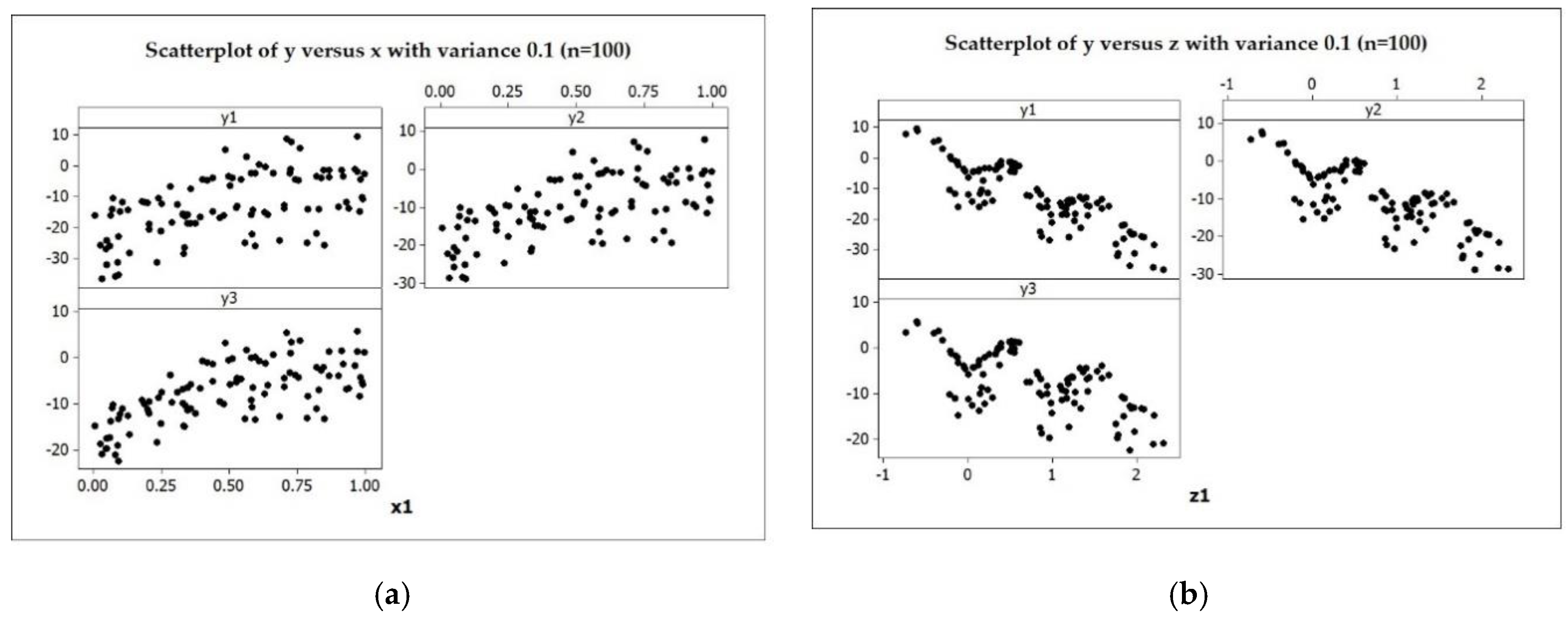
3.4. Simulation Study

Simulations with 100 replications were carried out to verify and validate the theoretical result of the proposed model. Using three data sample sizes ( n = 20, 50, and 100) and three different error variances ( σ 2 = 0.1, 0.5, and 1), random data were generated for multiresponse nonparametric regression. As shown in Figure 1, each predictor variable describes different functions, i.e., a polynomial function represents the truncated spline ( x i ), while a trigonometry function with a trend represents the Fourier series function ( z i ). As a note, Figure 1 only presents a partial scatterplot of the numerical example function for n = 100 and σ 2 = 0.1. The simulation study followed the model in Equation (4), so the polynomial and trigonometric functions used in this numerical example were obtained from the following function:
y 1 i = 15 ( x i 1 ) ( 1 x i ) 2 10.5 z i 4 cos ( 2 π z i ) + ε 1 i
y 2 i = 14 ( x i 1 ) ( 1 x i ) 2 7.5 z i 4 cos ( 2 π z i ) + ε 2 i
y 3 i = 13 ( x i 1 ) ( 1 x i ) 2 4.5 z i 4 cos ( 2 π z i ) + ε 3 i
In particular, the predictor variables x i and z i are generated from a Uniform (0,1) distribution, while random errors ε h i are generated from a multivariate normal distribution. In addition, ε 1 i , ε 2 i , and ε 3 i are correlated with c o r r   ( ε 1 i , ε 2 i ) = c o r r   ( ε 1 i , ε 3 i ) = c o r r   ( ε 2 i , ε 3 i ) = ρ = 0.9 . In order for ease of the computational process and based on the results of the partial scatterplot identification from Figure 1, the simulation study was carried out with the combination of three knots (K = 1, 2, 3) and three oscillation parameters (T = 1, 2, 3). To determine the optimal smoothing parameter, the minimum GCV criteria were used.
Table 1 provides a comparison of the statistical results for n = 100 with the error variances, the number of knots, and oscillation parameters. A complete summary of the statistical results for n = 20 and 50 is provided in Appendix G. Table 1 shows that the smallest GCV (6.098) occurs for variance σ 2 = 0.1 with the combination of the three knots–three oscillation model. This model yields adequate results, with coefficient of determination (R2) = 93,202 and mean-square-error (MSE) = 5.675. Surprisingly, the same result is seen for the other sample sizes ( n = 20 and 50), where the smallest GCV is obtained for variance σ 2 = 0.1. In addition, a comparison between sample sizes gives the result in which the smallest GCV is gained from the simulation with the largest sample number ( n = 100). Thus, a smaller variance with a large sample size will produce a minimum GCV, which implies that the regression curve will be better estimated as well. These findings are consistent with [23], who developed mixed estimators in nonparametric regression for cross-sectional data.

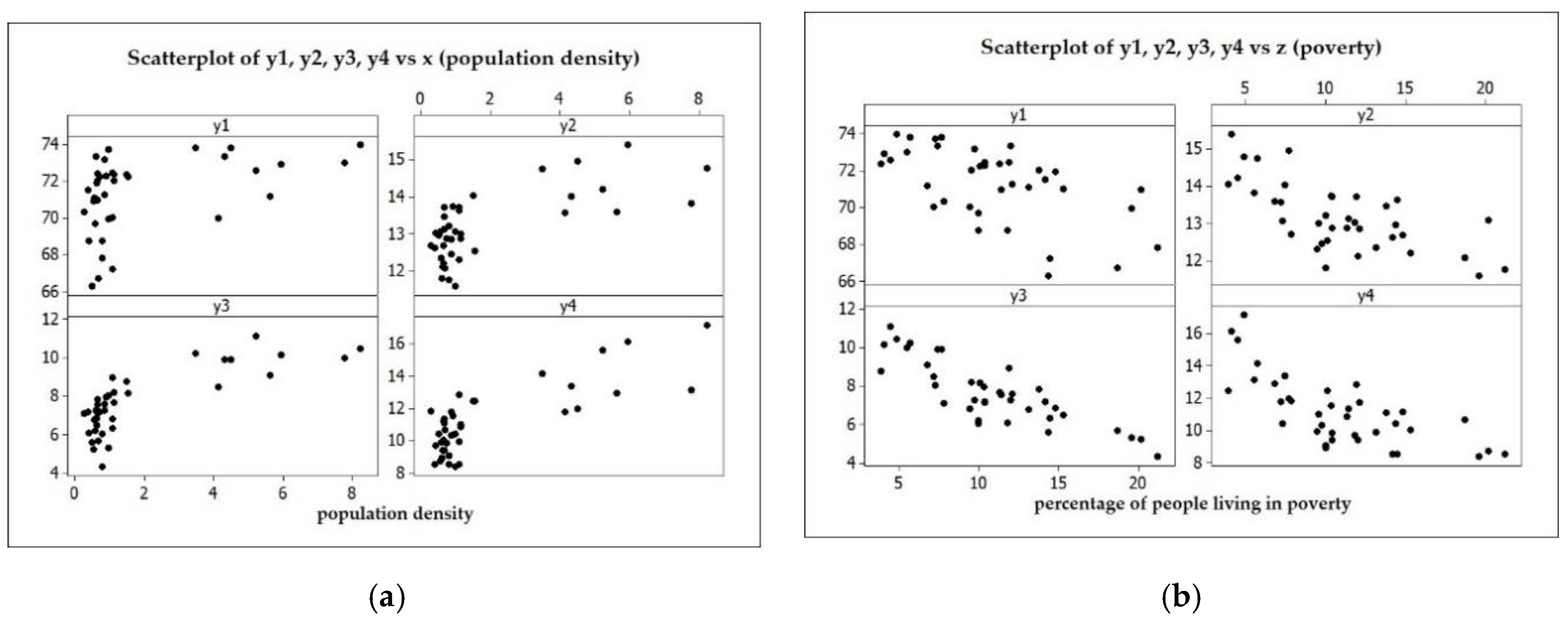
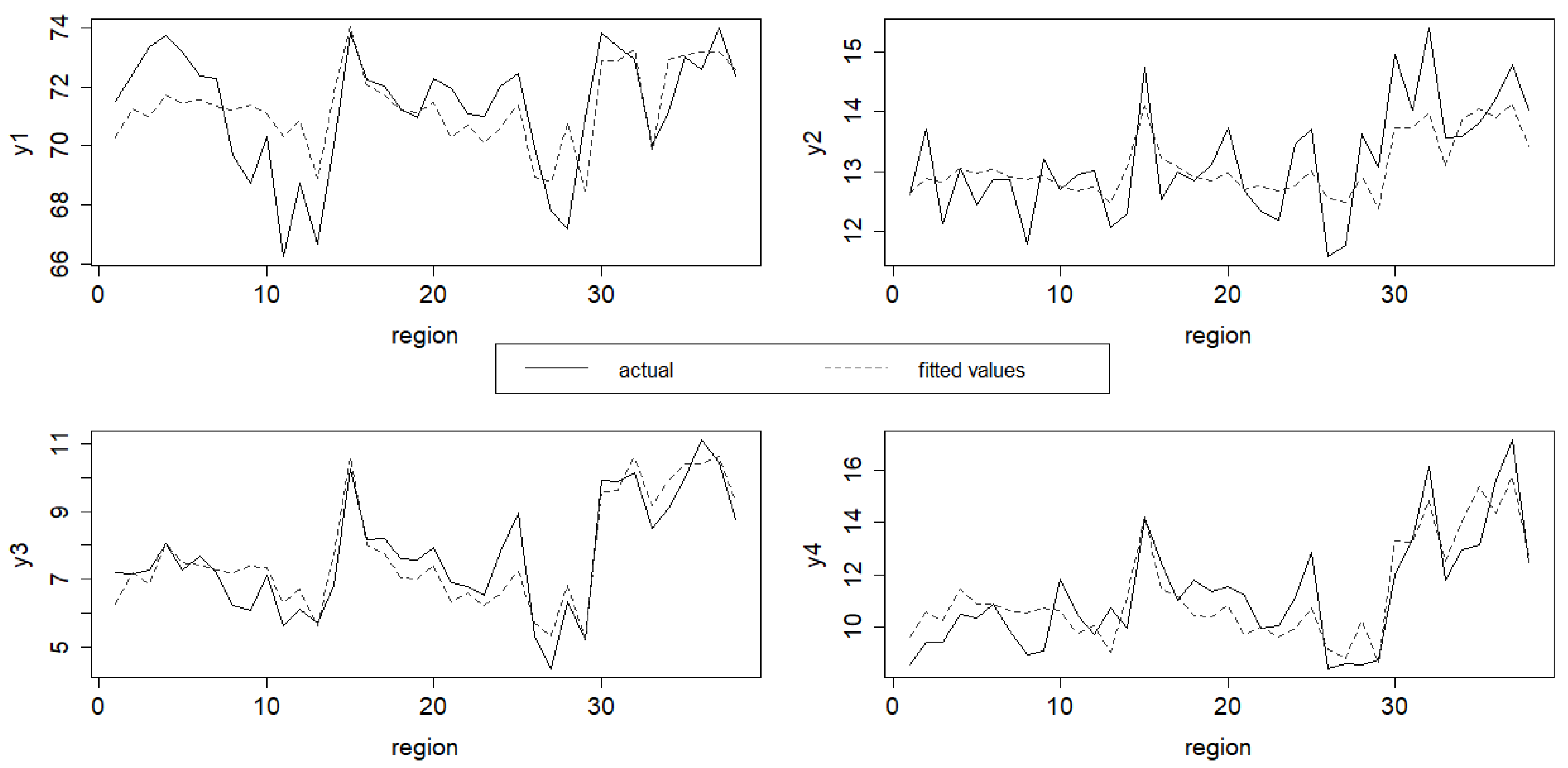
3.5. Data Application

This section attempts to provide the application of the proposed model to a real dataset. The proposed model was applied to four indicators of HDI data in 38 regencies/cities across East Java Province, Indonesia, in 2018. To measure human development in some regions, the UNDP developed the HDI in 1990. In the 1990 Human Development Report, three basic dimensions of human development were defined in the HDI: income (economy), health, and education [35]. From these dimensions, four indicators of HDI data were derived: life expectancy rate, expected years of schooling, mean years of schooling, and adjusted per capita expenditure [35]. In this study, these four indicators are the response variables, y 1 ,   y 2 , y 3 , and y 4 , respectively.
The issue of the HDI has received considerable critical attention in every province/regency in Indonesia as it is one of the determining components of the general allocation fund (DAU) [36]. As one of the largest provinces in Indonesia, East Java Province contributes significantly to Indonesia’s HDI. East Java Province’s HDI in 2018 was 70.77 [37], slightly lower than the national achievement. In addition, it was the lowest among the five other provinces of Java island in the last three years. Therefore, further studies on East Java Province’s HDI are to be potentially discussed.
To determine whether the correlation matrix has an identity matrix (homogeneity of variances), we used Bartlett’s test of sphericity with statistical significance α = 0.05. The results showed a statistical value of χ 2   = 121.993 with p-value = 0.00, which means that the decision was to reject the null hypothesis as p-value < α . According to this result, we can infer that there is a significant correlation among the response variables; hence, multiresponse nonparametric regression analysis can be used.
Several studies have highlighted the potential factors associated with Indonesia’s HDI, such as the percentage of people living in poverty [25,38], the unemployment rate [25,38,39], population density [25,38], and the per capita gross regional domestic product (GRDP) [25,39,40]. Based on these, the predictor variables used in this study were population density and the percentage of people living in poverty. In addition, the relationship between the response variable and each predictor variable was identified by a partial scatterplot, as shown in Figure 2. The partial scatter plot between the four indicators of the HDI and population density ( x ) showed changes at a particular subinterval that is fit for the truncated spline function. Meanwhile, the partial scatterplot between the response variable and the percentage of people living in poverty ( z ) followed a pattern that repeated at a certain interval, with a particular trend; thus, this variable was approached by the Fourier series function.
As shown in Table 2, some scenarios using a combined estimator (Model 1) and uncombined estimators (Model 2 and Model 3) were performed to compare the effectiveness of the proposed model. By using the modified GCV formula in Section 3.3, we selected the best model according to the minimum GCV as the criterion. In this study, a comparison of these three models revealed that the proposed model (Model 1) had the smallest GCV compared to the other uncombined estimator models for multiresponse nonparametric regression. In summary, these results indicate that the proposed model is better recommended for modeling the 2018 HDI data of East Java Province.
Another important result from Table 2 is the comparison of the number of knots and oscillation combinations from the proposed model. Similar to the simulation studies, we used a combination of three knot and oscillation parameters each. According to the minimum GCV as the criterion, the leading model was a three knots–three oscillations model with a GCV equal to 1.39189 and MSE = 1.08377. In addition, this model yields a coefficient of determination (R2) of 99.84%. Due to the satisfactory result of R2, it can be said that the proposed model is able to describe the variance of the response variable through the predictor variables exceptionally well. Another interesting result was the number of knot and oscillation combinations of the best model in the simulation study, in line with those of data application.
Appendix H presents the results of parameter estimation from the best model obtained from the minimum GCV in Table 2. As such, we obtained a three knots–three oscillations model. Based on the parameter estimation results for each response variable for the 2018 HDI data of East Java Province, Indonesia, the multiresponse nonparametric regression model with a combined truncated spline and Fourier series estimator can be written as
y ^ 1 = 0.932 + 0.869 x 1 i 3057.409   ( x 1 i 3.718 ) + + 6107.433   ( x 1 i 3.933 ) + 3050.878   ( x 1 i 4.148 ) + 0.677   z 1 i + 1 / 2 ( 1355.724 ) 935.001 cos z 1 i + 423.443 cos 2 z 1 i 92.348   cos 3 z 1 i . = 676.929 + 0.869 x 1 i 3057.409   ( x 1 i 3.718 ) + + 6107.433   ( x 1 i 3.933 ) + 3050.878   ( x 1 i 4.148 ) + 0.677   z 1 i 935.001 cos z 1 i + 423.443 cos 2 z 1 i 92.348   cos 3 z 1 i .
y ^ 2 = 0.747 + 0.393 x 1 i 619.153   ( x 1 i 3.718 ) + + 1235.608   ( x 1 i 3.933 ) + 616.769   ( x 1 i 4.148 ) + 0.180   z 1 i + 1 / 2 ( 274.146 ) 189.489 cos z 1 i + 85.224 cos 2 z 1 i 18.760   cos 3 z 1 i . = 136.326 + 0.393 x 1 i 619.153   ( x 1 i 3.718 ) + + 1235.608   ( x 1 i 3.933 ) + 616.769   ( x 1 i 4.148 ) + 0.180   z 1 i 189.489 cos z 1 i + 85.224 cos 2 z 1 i 18.760 cos 3 z 1 i .
y ^ 3 = 0.102 + 0.865 x 1 i 510.292   ( x 1 i 3.718 ) + + 1015.208   ( x 1 i 3.933 ) + 505.678   ( x 1 i 4.148 ) + 0.411   z 1 i + 1 / 2 ( 224.955 ) 156.440 cos z 1 i + 69.027 cos 2 z 1 i 15.588   cos 3 z 1 i . = 112.375 + 0.865 x 1 i 510.292   ( x 1 i 3.718 ) + + 1015.208   ( x 1 i 3.933 ) + 505.678   ( x 1 i 4.148 ) + 0.411   z 1 i 156.440 cos z 1 i + 69.027 cos 2 z 1 i 15.588   cos 3 z 1 i .
y ^ 4 = 0.482 + 0.969 x 1 i 684.712   ( x 1 i 3.718 ) + + 1363.397   ( x 1 i 3.933 ) + 679.163   ( x 1 i 4.148 ) + 0.456   z 1 i + 1 / 2 ( 302.146 ) 209.894 cos z 1 i + 92.927 cos 2 z 1 i 20.891   cos 3 z 1 i . = 150.591 + 0.969 x 1 i 684.712   ( x 1 i 3.718 ) + + 1363.397   ( x 1 i 3.933 ) + 679.163   ( x 1 i 4.148 ) + 0.456   z 1 i 209.894 cos z 1 i + 92.927 cos 2 z 1 i 20.891   cos 3 z 1 i .
Figure 3 presents a comparison between the response variable and the fitted values using the proposed model. From the graph, we can see that all fitted values resemble the pattern of the real data; although some do not, there are only a few deviations. Thus, the proposed model can produce a prediction model.

4. Discussion and Conclusions

This study presents the major findings from regression curve estimation with a combined truncated spline and Fourier series estimator for an additive model in multiresponse nonparametric regression using PWLS and WLS optimization, as shown below:
f ^ ( K , λ , T ) ( x , z ) = J [ J T ( I 2 H T ) W J + J T H T W H J ] 1 [ J T ( H T I ) W ( H I ) ] y ,
g ^ ( K , λ , T ) ( x , z ) = Z ( [ Z T W Z + N D ( λ ) ] 1 Z T W ( I J K 1 L ) y ) ,
μ ^ ( K , λ , T ) ( x , z ) = [ J K 1 L + H ( I J K 1 L ) ] y
Furthermore, the result of error variance–covariance matrix estimation is as follows:
W ^ = ( σ ^ 11 σ ^ 12 σ ^ 1 r σ ^ 12 σ ^ 22 σ ^ 2 r σ ^ 1 r σ ^ 2 r σ ^ r r ) I
From the simulation study, the minimum GCV obtained a satisfactory outcome through a large sample with small variance. In addition, data application to a real dataset of the 2018 HDI in East Java revealed that the proposed model had a better result than the uncombined model. An adequate coefficient of determination (R2) from the best model indicates that the proposed model can explain the data variation remarkably well. Interestingly, the number of knots and oscillations of the best model in this simulation study and data application is consistent; that is a combination of three knots–three oscillations. In summary, these findings have significant implications for the understanding of regression curve estimation when using combined estimators for multiresponse nonparametric regression. Although the focus of the research was on combined truncated spline and Fourier series estimators, the procedure in this study can be applied to other combinations of estimators for multiresponse nonparametric regression.
The scope of this study was limited in terms of curve estimation and estimation of the variance–covariance matrix; thus, the major limitation was the absence of hypothesis testing and confidence intervals testing. Considering its necessity for good statistical practice, there is a commitment to perform such a goodness-of-fit test (model checking). Therefore, further research will be conducted to achieve hypothesis testing and confidence intervals testing. Another possible area is that a further simulation study could be performed using another function, such as an exponential or logarithmic function, to validate the capability of the proposed model. An additional variation of ρ in a simulation study could be used to gain more insights into the performance evaluation of the proposed model.

Author Contributions

Conceptualization, H.N., I.N.B., and I.Z.; methodology, H.N. and I.N.B.; writing—original draft preparation, H.N.; writing—review and editing, H.N., I.N.B., and I.Z. All authors have read and agreed to the published version of the manuscript.

Funding

H.N. thanks BPS—Statistics Indonesia, which has bestowed a doctoral scholarship through APBN BPS. This research was funded by Deputi Bidang Penguatan Riset dan Pengembangan, Ministry of Research and Technology/National Research and Innovation Agency (Kemenristek or RISTEK-BRIN), the Republic of Indonesia, via grant Penelitian Disertasi Doktor (PDD) in 2021.

Institutional Review Board Statement

Not applicable.

Informed Consent Statement

Not applicable.

Data Availability Statement

Publicly available datasets were analyzed in this study. This data can be found here: BPS—Statistics of Jawa Timur Province, Indonesia, https://jatim.bps.go.id, accessed on 1 March 2021.

Conflicts of Interest

The authors declare no conflict of interest.

Abbreviations

GoFgoodness-of-fit
GCVgeneralized cross-validation
MSEmean square error
MLEmaximum likelihood estimation
OLSordinary least square
PLSpenalized least square
PWLSpenalized weighted least square
WLSweighted least square

Appendix A

Lemma 1 can be proven by the completed R ( g h k ( z k 1 ) , g h k ( z k 2 ) , , g h k ( z k n ) ) as the GoF of PWLS optimization in Equation (7), as shown below:
R ( g h k ( z k 1 ) , g h k ( z k 2 ) , , g h k ( z k n ) ) = N 1 h = 1 r i = 1 n w h i ( y h i j = 1 p f h j ( x j i ) k = 1 q g h k ( z k i ) ) 2 .
If v h i = y h i j = 1 p f h j ( x j i ) , then Equation (A1) can be written as
R ( g h k ( z k 1 ) , g h k ( z k 2 ) , , g h k ( z k n ) ) = N 1 h = 1 r i = 1 n w h i ( v h i k = 1 q g h k ( z k i ) ) 2 ,
where g h k ( z k i ) is the Fourier series function, as shown in Equation (6). Furthermore, the function g h k ( z k i ) with one predictor variable, symbolized as k , can be written in the following matrix form:
g h = [ g h k ( z k 1 ) g h k ( z k 2 ) g h k ( z k n ) ] = [ b h k z k 1 + 1 2 a 0 h k + a 1 h k cos 1 z k 1 + a 2 h k cos 2 z k 1 + + a T h k cos T z k 1 b h k z k 2 + 1 2 a 0 h k + a 1 h k cos 1 z k 2 + a 2 h k cos 2 z k 2 + + a T h k cos T z k 2 b h k z k n + 1 2 a 0 h k + a 1 h k cos 1 z k n + a 2 h k cos 2 z k n + + a T h k cos T z k n ]
= [ z k 1 1 / 2 cos 1 z k 1 cos 2 z k 1 cos 1 z k 1 z k 2 1 / 2 cos 1 z k 2 cos 2 z k 2 cos T z k 2 z k n 1 / 2 cos 1 z k n cos 2 z k n cos T z k n ] [ b h k a 0 h k a 1 h k a 2 h k a T h k ]
= Z k a h k
Similarly, for k = 1 , 2 , , q predictors, the Fourier series function for the multiresponse nonparametric regression presented in Equation (A3) can be written as
g h = Z 1 a h 1 + Z 2 a h 2 + + Z q a h q
= k = 1 q Z k a h k = Z h a h ,
such that
g = [ g 1 T g 2 T g r T ] = [ Z 1 a 1 Z 2 a 2 Z r a r ] = [ Z 1 0 0 0 Z 2 0 0 0 Z r ] [ a 1 a 2 a r ] = Z a
Thus, the GoF in Equation (7), where g h k ( z k i ) is the Fourier series function, can be expressed as
R ( g h k ( z k 1 ) , g h k ( z k 2 ) , , g h k ( z k n ) ) = N 1 h = 1 r i = 1 n w h i ( v h i k = 1 q g h k ( z k i ) ) 2
= N 1 h = 1 r i = 1 n w h i ( v h i k = 1 q ( b h k z k i + 1 2 a 0 h k + t = 1 T a t h k cos t z k i ) ) 2 .
As a result, the GoF component in Equation (A5) can be drawn in the following matrix form:
R ( g 1 , , g r ) = N 1 W ( v Z a ) 2
= N 1 ( v Z a ) T W ( v Z a ) .

Appendix B

The penalty component of the PWLS optimization in Equation (7) is as follows:
k = 1 q λ k 0 π 2 π ( g k ( z k ) ) 2 d z k ,
where g h k ( z k i ) is presented in Equation (6). To prove Lemma 2, let us begin with solving the second derivative in Equation (A6), as follows:
0 π 2 π ( g k ( z k ) ) 2 d z k = 0 π 2 π ( d d z k [ d d z k ( b h k z k i + 1 2 a 0 h k + t = 1 T a t h k cos t z k i ) ] ) 2 d z k
= 2 π 0 π ( t = 1 T t 2   a t h k cos t z k i ) 2 d z k
= 2 π 0 π { t = 1 T ( t 2   a t h k cos t z k i ) 2 + 2 t < u T ( t 2   a t h k cos t z k i ) ( u 2   a t h k cos u z k i ) } d z k
= 2 π t = 1 T 0 π ( t 4   a t h k 2 cos 2 t z k i )   d z k + 4 π 0 π t < u T ( ( t u ) 2   a t h k cos t z k i a u h k cos u z k i ) d z k  
= t = 1 T t 4   a t h k 2 .
After obtaining the result in Equation (A7), the solution to the penalty component in Equation (A6) can be written as
P ( λ 1 , λ 2 , , λ q ) = k = 1 q λ k 0 π 2 π ( g k ( z k ) ) 2 d z k
= k = 1 q ( λ k t = 1 T t 4 a t h k 2 )
= a T D ( λ ) a   .

Appendix C

According to the result of the GoF in Lemma 1 and the penalty in Lemma 2, the PWLS optimization in Equation (7) can be written as
Min g k C [ 0 , π ] { N 1 h = 1 r i = 1 n w h i ( y h i j = 1 p f h j ( x j i ) k = 1 q g h k ( z k i ) ) 2 + k = 1 q λ k 0 π 2 π ( g k ( z k ) ) 2 d z k }
= M i n a R ( 2 + T ) q h x 1 { N 1 ( v Z a ) T W ( v Z a ) + a T D ( λ ) a }
If F ( a ) = N 1 ( v Z a ) T W ( v Z a ) + a T D ( λ ) a , then
F ( a ) = N 1 v T W v 2 N 1 a T Z T W v + N 1 a T Z T W Z a + a T D ( λ ) a ,
such that
M i n a R ( 2 + T ) q h x 1 { N 1 ( v Z a ) T W ( v Z a ) + a T D ( λ ) a }
= M i n a R ( 2 + T ) q h x 1 { N 1 v T W v 2 N 1 a T Z T W v + N 1 a T Z T W Z a + a T D ( λ ) a } .
To solve the optimization in Equation (A8), the estimator a ^ can be obtained by deriving the partial Equation (A8) against a and equating the result with 0, as follows:
F ( a ) a = [ N 1 v T W v 2 N 1 a T Z T W v + N 1 a T Z T W Z a + a T D ( λ ) a ] a
a ^ = [ Z T W Z + N D ( λ ) ] 1 Z T W v .
The subsequent step is to substitute a ^ in Equation (A9) into Equation (A4), such that the estimator of the truncated spline function can be written as
g ^ ( K , λ , T ) ( x , z ) = Z a ^
= ( Z [ Z T W Z + N D ( λ ) ] 1 Z T W ) v
= H v .

Appendix D

The solution in Theorem 1 still contains an f component, where f is a truncated linear spline function, as described in Equation (5). Hence, to complete the PWLS optimization in Equation (7), it is necessary to estimate the regression curve of f h j ( x j i ) . First, the multiresponse nonparametric regression curve of the truncated spline component in Equation (5), which involves only one predictor, is written in the following matrix form:
f h = [ f h j ( x j 1 ) f h j ( x j 2 ) f h j ( x j n ) ] = [ α h j x j 1 + s = 1 u β h j s ( x j 1 K h j s ) + α h j x j 2 + s = 1 u β h j s ( x j 2 K h j s ) + α h j x j n + s = 1 u β h j s ( x j n K h j s ) + ]
= [ x j 1 x j 2 x j n ] α h j + [ ( x j 1 K h j 1 ) + ( x j 1 K h j 2 ) + ( x j 1 K h j u ) + ( x j 2 K h j 1 ) + ( x j 2 K h j 2 ) + ( x j 2 K h j u ) + ( x j n K h j 1 ) + ( x j n K h j 2 ) + ( x j n K h j u ) + ] [ β h j 1 β h j 2 β h j u ]
= x j i α h j + S j i β h j
Consequently, f h with the j = 1 , 2 , , p predictor can be written as follows:
f h = x 1 i α 1 h + S 1 i β 1 h + x 2 i α 2 h + S 2 i β 2 h + + x p i α p h + S p i β p h
= X i α h + S i β h ,
According to Equation (A13), the truncated spline function for multiresponse nonparametric regression can be expressed in matrix form, as follows:
f = [ f 1 T f 2 T f r T ] = [ X 1 α 1 X 2 α 2 X r α r ] + [ S 1 β 1 S 2 β 2 S r β r ] = [ X 1 0 0 0 X 2 0 0 0 X r ] [ α 1 α 2 α r ] + [ S 1 0 0 0 S 2 0 0 0 S r ] [ β 1 β 2 β r ]
= [ X 1 0 0 0 X 2 0 0 0 X r | S 1 0 0 0 S 2 0 0 0 S r ] [ α 1 α 2 α r β 1 β 2 β r ]
= [ X | S ] [ α β ] = J γ .
To solve the regression curve estimation of the truncated spline and Fourier series estimators for multiresponse nonparametric regression with PWLS optimization, substitute Equations (A11) and (A14) into Equation (4), as follows:
y = f + g + ε ;   g = H v
ε = y f H v ;   v = y f
= y f H ( y f ) ;   f = J γ
= ( I H ) ( y J γ ) .
The subsequent step is to solve Equation (A15) with WLS optimization. Therefore, the estimator can be obtained by completing the following WLS:
ε T ε = [ ( I H ) ( y J γ ) ] T W [ ( I H ) ( y J γ ) ]

Appendix E

The second stage of the proposed method is performed using WLS optimization, as follows:
Min γ R ( 1 + u ) n r { [ ( I H ) ( y J γ ) ] T W [ ( I H ) ( y J γ ) ] }
If T ( γ ) = [ y H y J γ + H J γ ] T W [ y H y J γ + H J γ ] , then we perform the multiplication in parentheses to obtain,
T ( γ ) = y T W y + y T H T W H y + γ T J T W J γ + γ T J T H T W H J γ 2 y T H T W y 2 γ T J T W y + 2 γ T J T H T W y + 2 γ T J T W H y 2 γ T J T H T W H y 2 γ T J T H T W J γ .
WLS optimization can be obtained by partial derivation of T ( γ ) against γ . When the expression is equal to 0, the result is Equation (A16):
T ( γ ) γ = γ ( y T W y + y T H T W H y + γ T J T W J γ + γ T J T H T W H J γ 2 y T H T W y 2 γ T J T W y + 2 γ T J T H T W y + 2 γ T J T W H y 2 γ T J T H T W H y 2 γ T J T H T W J γ ) = 0 ,
γ ^ = [ J T ( I 2 H T ) W J + J T H T W H J ] 1 [ J T ( H T I ) W ( H I ) ] y .
Substituting Equation (A16) into Equation (A14) yields
f ^ ( K , λ , T ) ( x , z ) = J γ ^
= J [ J T ( I 2 H T ) W J + J T H T W H J ] 1 [ J T ( H T I ) W ( H I ) ] y
= J K 1 L y .

Appendix F

Assume random error ε in Equation (2) is normally distributed with mean 0 and error variance–covariance matrix W such that it can be written as ε ~ N ( 0 , W ) . Thus, matrix W is outlined as follows
W = V a r ( ε ) = E [ ( ε E ( ε ) ) ( ε E ( ε ) ) T ]
= E [ ( ε 11 , ε 12 , , ε 1 n , ε 21 , ε 22 , , ε 2 n , , ε r 1 , ε r 2 , , ε r n ) T ( ε 11 , ε 12 , , ε 1 n , ε 21 , ε 22 , , ε 2 n , , ε r 1 , ε r 2 , , ε r n ) ]
= E ( ε 11 2 ε 11 ε 12 ε 11 ε 1 n ε 11 ε 21 ε 11 ε 22 ε 11 ε 2 n ε 11 ε r 1 ε 11 ε r 2 ε 11 ε r n ε 12 ε 11 ε 12 2 ε 12 ε 1 n ε 12 ε 21 ε 12 ε 22 ε 12 ε 2 n ε 12 ε r 1 ε 12 ε r 2 ε 12 ε r n ε 1 n ε 11 ε 21 ε 12 ε 1 n 2 ε 1 n ε 21 ε 1 n ε 22 ε 1 n ε 2 n ε 1 n ε r 1 ε 1 n ε r 2 ε 1 n ε r n ε 21 ε 11 ε 21 ε 12 ε 21 ε 1 n ε 21 2 ε 21 ε 22 ε 21 ε 2 n ε 21 ε r 1 ε 21 ε r 2 ε 21 ε r n ε 22 ε 11 ε 22 ε 12 ε 22 ε 1 n ε 22 ε 21 ε 22 2 ε 22 ε 2 n ε 22 ε r 1 ε 22 ε r 2 ε 22 ε r n ε 2 n ε 11 ε 2 n ε 12 ε 2 n ε 1 n ε 2 n ε 21 ε 2 n ε 22 ε 2 n 2 ε 2 n ε r 1 ε 2 n ε r 2 ε 2 n ε r n ε r 1 ε 11 ε r 1 ε 12 ε r 1 ε 1 n ε r 1 ε 21 ε r 1 ε 22 ε r 1 ε 2 n ε r 1 2 ε r 1 ε r 2 ε r 1 ε r n ε r 2 ε 11 ε r 2 ε 12 ε r 2 ε 1 n ε r 2 ε 21 ε r 2 ε 22 ε r 2 ε 2 n ε r 2 ε r 1 ε r 2 2 ε r 2 ε r n ε r n ε 11 ε r n ε 12 ε r n ε 1 n ε r n ε 21 ε r n ε 22 ε r n ε 2 n ε r n ε r 1 ε r n ε r 2 ε r n 2 ) .
The correlation between response variables, define as c o r r ( ε h i ε i ) , is assumed to be constant as ρ for all response variables and succeeded by the other assumptions, as follows:
E ( ε h i ε h i ) = { σ h h ,   i f   i = i 0 ,   i f   i i   w h e r e   h = 1 , 2 , , r E ( ε h i ε i ) = { σ h ,   i f   i = i 0 ,   i f   i i   w i t h   σ h = ρ σ h h σ
According to the above assumption, Equation (A19) can be written as
W = ( σ 11 σ 12 σ 1 r σ 12 σ 22 σ 2 r σ 1 r σ 2 r σ r r ) I
= Σ I
The estimation of matrix W is obtained by the maximum likelihood estimation (MLE) method, as in Equation (A20). Furthermore, substitute Equation (A10) and Equation (A17) into μ ( x , z ) ; then, the likelihood presented in Equation (A22) is as follows:
L ( W | μ , y ) = ( 2 π ) r n / 2 | W | n / 2 exp [ 1 2 i = 1 n ( ( y μ ( x , z ) ) T W 1 ( y μ ( x , z ) ) ) ]
= ( 2 π ) r n / 2 | W | n / 2 exp [ 1 2 i = 1 n ( ( y ( J γ + Z a ) ) T W 1 ( y ( J γ + Z a ) ) ) ] .
By taking the natural logarithm from the likelihood function and substituting W , as in Equation (A20), the result is as follows:
ln L ( Σ ) = r n 2 ln ( 2 π ) n 2 ln | Σ I | 1 2 i = 1 n [ ( y ( J γ + Z a ) ) T ( Σ I ) 1 ( y ( J γ + Z a ) ) ]
Point ( y ( J γ + Z a ) ) into the form of v e c ( C )
( y ( J γ + Z a ) ) T ( Σ I ) 1 ( y ( J γ + Z a ) ) = ( v e c ( C ) ) T ( Σ I ) 1 ( v e c ( C ) ) = t r ( Σ 1 C T C )
such that Equation (A23) can be written as
ln L ( Σ | γ , a , y ) = r n 2 ln ( 2 π ) n 2 ln | Σ | 1 2 t r ( Σ 1 C T C )  
The maximum value of the likelihood function is obtained by partially deriving Equation (A24) against σ h and equating the result with 0, as follows:
σ h ln L ( Σ ^ | γ , a , y ) = n 2 ( σ h ln | Σ ^ | ) 1 2 σ h t r ( Σ ^ 1 C T C ) = 0
such that
Σ ^ = 1 n ( C T C )  
= ( [ y 1 ( J γ + Z a ) ] T [ y 1 ( J γ + Z a ) ] n [ y 1 ( J γ + Z a ) ] T [ y 2 ( J γ + Z a ) ] n [ y 1 ( J γ + Z a ) ] T [ y r ( J γ + Z a ) ] n [ y 1 ( J γ + Z a ) ] T [ y 2 ( J γ + Z a ) ] n [ y 2 ( J γ + Z a ) ] T [ y 2 ( J γ + Z a ) ] n [ y 2 ( J γ + Z a ) ] T [ y r ( J γ + Z a ) ] n [ y 1 ( J γ + Z a ) ] T [ y r ( J γ + Z a ) ] n [ y 2 ( J γ + Z a ) ] T [ y r ( J γ + Z a ) ] n [ y r ( J γ + Z a ) ] T [ y r ( J γ + Z a ) ] n )
The subsequent step is to estimate γ and a using the ordinary least square (OLS) method, with the result as follows:
γ = [ y T y 2 γ T J T y 2 a T Z T y + 2 a T Z T J γ + γ T J T J γ + a T Z T Z a ] γ
γ ^ s = ( ( [ I ( J T J ) 1 J T Z ( Z T Z ) 1 Z T J ] 1 ( J T J ) 1 J T ) ( ( J T J ) 1 J T Z ( Z T Z ) 1 Z T ) ) y = F y
a = [ y T y 2 γ T J T y 2 a T Z T y + 2 a T Z T J γ + γ T J T J γ + a T Z T Z a ] a
a ^ s = ( ( [ I ( Z T Z ) 1 Z T J ( J T J ) 1 J T Z ] 1 ( Z T Z ) 1 Z T ) ( ( Z T Z ) 1 Z T J ( J T J ) 1 J T ) ) y = G y
Substituting the result of γ ^ s and a ^ s above into Equation (A25), error variance–covariance matrix W in Equation (A20) can be written as follows:
W ^ = Σ ^ I ,  
where
σ ^ 11 = [ y 1 ( J F + Z G ) y 1 ] T [ y 1 ( J F + Z G ) y 1 ] n ,   σ ^ 22 = [ y 2 ( J F + Z G ) y 2 ] T [ y 2 ( J F + Z G ) y 2 ] n ,   σ ^ r r = [ y r ( J F + Z G ) y r ] T [ y r ( J F + Z G ) y r ] n ,
σ ^ 12 = [ y 1 ( J F + Z G ) y 1 ] T [ y 2 ( J F + Z G ) y 2 ] n ,   σ ^ 1 r = [ y 1 ( J F + Z G ) y 1 ] T [ y r ( J F + Z G ) y r ] n ,   σ ^ 2 r = [ y 2 ( J F + Z G ) y 2 ] T [ y r ( J F + Z G ) y r ] n

Appendix G

Table A1. Summary of statistical results for n = 20 and 50 with error variances, the number of knots, and oscillation parameters.
VarianceNumber of OscillationsNumber of Knotsn = 20n = 50
GCVR2MSEGCVR2MSE
0.1117.02388.6654.5277.20790.1706.735
26.85989.8664.0806.84890.6076.312
36.47091.6723.3366.685 *91.1726.075
216.77787.6495.0367.07491.1335.960
26.386 *88.2884.7126.97291.6095.638
36.38889.8814.0857.16591.8355.489
316.53586.3985.2947.07491.1335.959
26.60188.1125.1516.97291.6105.638
36.61787.9294.9707.16691.8335.489
0.5119.18593.2805.6679.21790.9527.783
210.01093.3035.6557.14193.2935.769
310.13993.8245.2197.26593.3845.692
217.97092.4706.4559.21590.9337.797
28.19392.5386.3937.13393.2845.775
38.01292.8966.0187.29393.4365.645
3110.77292.2106.5999.21590.9307.799
29.26393.3285.6557.13293.2835.776
38.39692.5576.3067.29393.4335.647
1.0119.25692.9355.7197.55994.7347.064
210.13693.2185.4917.31994.9726.746
310.24193.7515.0586.89095.3326.262
218.01991.9886.4957.58595.2276.401
27.83892.5186.1167.46195.5086.024
37.33093.4455.5067.38095.7535.698
3110.59391.6666.7637.49094.8626.903
27.66892.6295.9837.17595.1556.521
38.69793.8335.0136.96895.3516.245
* The smallest value of GCV.

Appendix H

Table A2. Results of parameter estimation of the best model.
Response VariableParameterEstimationResponse VariableParameterEstimation
y 1 α 01 −0.932 y 3 α 03 −0.102
α 11 0.869 α 31 0.865
β 111 −3057.409 β 311 −510.292
β 112 6107.433 β 312 1015.208
β 113 −3050.878 β 313 −505.678
b 11 −0.677 b 31 −0.411
a 011 1355.724 a 031 224.955
a 111 −935.001 a 311 −156.440
a 112 423.443 a 312 69.027
a 113 −92.348 a 313 −15.588
y 2 α 02 −0.747 y 4 α 04 −0.482
α 21 0.393 α 41 0.969
β 211 −619.153 β 411 −684.712
β 212 1235.608 β 412 1363.397
β 213 −616.769 β 413 −679.163
b 21 −0.180 b 41 −0.456
a 021 274.146 a 041 302.146
a 211 −189.489 a 411 −209.894
a 212 85.224 a 412 92.927
a 213 −18.760 a 413 −20.891

References

  1. Härdle, W. Applied Nonparametric Regression; Cambridge University Press: Cambridge, UK, 1990. [Google Scholar]
  2. Eubank, R.L. Nonparametric Regression and Spline Smoothing, 2nd ed.; Marcel Dekker, Inc.: New York, NY, USA, 1999. [Google Scholar]
  3. Budakçı, G.; Oruç, H. Further Properties of Quantum Spline Spaces. Mathematics 2020, 8, 1770. [Google Scholar] [CrossRef]
  4. Du, R.; Yamada, H. Principle of Duality in Cubic Smoothing Spline. Mathematics 2020, 8, 1839. [Google Scholar] [CrossRef]
  5. Lapshin, V. A nonparametric approach to bond portfolio immunization. Mathematics 2019, 7, 1121. [Google Scholar] [CrossRef] [Green Version]
  6. Nurcahayani, H.; Budiantara, I.N.; Zain, I. Nonparametric Truncated Spline Regression on Modelling Mean Years Schooling of Regencies in Java. AIP Conf. Proc. 2019, 2194, 020073. [Google Scholar] [CrossRef]
  7. Yu, W.; Yong, Y.; Guan, G.; Huang, Y.; Su, W.; Cui, C. Valuing guaranteed minimum death benefits by cosine series expansion. Mathematics 2019, 7, 835. [Google Scholar] [CrossRef] [Green Version]
  8. Kim, J.; Hart, J.D. A Change-Point Estimator Using Local Fourier series. J. Nonparametr. Stat. 2011, 23, 83–98. [Google Scholar] [CrossRef]
  9. Bilodeau, M. Fourier Smoother and Additive Models. Can. J. Stat. 1992, 20, 257–269. [Google Scholar] [CrossRef]
  10. Yang, Y.; Pilanci, M.; Wainwright, M.J. Randomized Sketches for Kernels: Fast and Optimal Nonparametric Regression. Ann. Stat. 2017, 45, 991–1023. [Google Scholar] [CrossRef] [Green Version]
  11. Zhao, G.; Ma, Y. Robust Nonparametric Kernel Regression Estimator. Stat. Probab. Lett. 2016, 116, 72–79. [Google Scholar] [CrossRef]
  12. Kayri, M.; Zırhlıoğlu, G. Kernel Smoothing Function and Choosing Bandwidth for Non-Parametric Regression Methods. Ozean J. Appl. Sci. 2009, 2, 49–54. [Google Scholar]
  13. Syengo, C.K.; Pyeye, S.; Orwa, G.O.; Odhiambo, R.O. Local Polynomial Regression Estimator of the Finite Population Total under Stratified Random Sampling: A Model-Based Approach. Open J. Stat. 2016, 6, 1085–1097. [Google Scholar] [CrossRef] [Green Version]
  14. Chamidah, N.; Budiantara, I.N.; Sunaryo, S.; Zain, I. Designing of Child Growth Chart Based on Multi-Response Local Polynomial Modeling. J. Math. Stat. 2012, 8, 342–347. [Google Scholar]
  15. Opsomer, J.D.; Ruppert, D. Fitting a Bivariate Additive Model by Local Polynomial Regression. Ann. Stat. 1997, 25, 186–211. [Google Scholar] [CrossRef]
  16. Maronge, J.M.; Zhai, Y.; Wiens, D.P.; Fang, Z. Optimal designs for spline wavelet regression models. J. Stat. Plan. Inference 2017, 184, 94–104. [Google Scholar] [CrossRef] [Green Version]
  17. Antoniadis, A.; Bigot, J.; Sapatinas, T. Wavelet estimators in nonparametric regression: A comparative simulation study. J. Stat. Softw. 2001, 6, 1–83. [Google Scholar] [CrossRef] [Green Version]
  18. Antoniadis, A.; Leblanc, F. Nonparametric Wavelet Regression for Binary Response. Statistics 2000, 34, 183–213. [Google Scholar] [CrossRef]
  19. Sifriyani; Budiantara, I.N.; Kartiko, S.H.; Gunardi. Evaluation of Factors Affecting Increased Unemployment in East Java Using NGWR-TS Method. Int. J. Sci. Basic Appl. Res. 2019, 46, 123–142. [Google Scholar]
  20. Sifriyani; Kartiko, S.H.; Budiantara, I.N.; Gunardi. Development of Nonparametric Geographically Weighted Regression using Truncated Spline Approach. Songklanakarin J. Sci. Technol. 2018, 40, 909–920. [Google Scholar]
  21. Budiantara, I.N.; Ratnasari, V.; Ratna, M.; Zain, I. The Combination of Spline and Kernel Estimator for Nonparametric Regression and Its Properties. Appl. Math. Sci. 2015, 9, 6083–6094. [Google Scholar] [CrossRef]
  22. Ratnasari, V.; Budiantara, I.N.; Ratna, M.; Zain, I. Estimation of Nonparametric Regression Curve using Mixed Estimator of Multivariable Truncated Spline and Multivariable Kernel. Glob. J. Pure Appl. Math. 2016, 12, 5047–5057. [Google Scholar]
  23. Hidayat, R.; Budiantara, I.N.; Otok, B.W.; Ratnasari, V. The regression curve estimation by using mixed smoothing spline and kernel (MsS-K) model. Commun. Stat. Theory Methods 2020. [Google Scholar] [CrossRef]
  24. Budiantara, I.N.; Ratnasari, V.; Ratna, M.; Wibowo, W.; Afifah, N.; Rahmawati, D.P.; Octavanny, M.A.D. Modeling Percentage of Poor People In Indonesia Using Kernel And Fourier Series Mixed Estimator In Nonparametric Regression. Rev. Investig. Operacional. 2019, 40, 538–550. [Google Scholar]
  25. Nurcahayani, H.; Budiantara, I.N.; Zain, I. The Semiparametric Regression Curve Estimation by Using Mixed Truncated Spline and Fourier Series Model. AIP Conf. Proc. 2021, 2329, 060025. [Google Scholar] [CrossRef]
  26. Mariati, N.P.A.M.; Budiantara, I.N.; Ratnasari, V. Combination Estimation of Smoothing Spline and Fourier Series in Nonparametric Regression. J. Math. 2020, 2020, 1–10. [Google Scholar] [CrossRef]
  27. Sudiarsa, I.W.; Budiantara, I.N.; Suhartono; Purnami, S.W. Combined Estimator Fourier Series and Spline Truncated in Multivariable Nonparametric Regression. Appl. Math. Sci. 2015, 9, 4997–5010. [Google Scholar] [CrossRef]
  28. Octavanny, M.A.D.; Budiantara, I.N.; Kuswanto, H.; Rahmawati, D.P. Nonparametric Regression Model for Longitudinal Data with Mixed Truncated Spline and Fourier Series. Abstr. Appl. Anal. 2020, 2020, 1–11. [Google Scholar] [CrossRef]
  29. Caldeira, J.F.; Gupta, R.; Torrent, H.S. Forecasting U.S. Aggregate Stock Market Excess Return: Do Functional Data Analysis Add Economic Value? Mathematics 2020, 8, 2042. [Google Scholar] [CrossRef]
  30. Correa-Quezada, R.; Cueva-Rodríguez, L.; Álvarez-García, J.; del Río-Rama, M.d.l.C. Application of the Kernel Density Function for the Analysis of Regional Growth and Convergence in the Service Sector through Productivity. Mathematics 2020, 8, 1234. [Google Scholar] [CrossRef]
  31. Green, P.J.; Silverman, B.W. Nonparametric Regression and Generalized Linear Models, 1st ed.; Chapman and Hall/CRC: New York, NY, USA, 1993. [Google Scholar]
  32. Wang, Y.; Guo, W.; Brown, M.B. Spline smoothing for bivariate data with applications to association between hormones. Stat. Sin. 2000, 10, 377–397. [Google Scholar]
  33. Wahba, G. Spline Models for Observational Data; SIAM Society For Industrial And Applied Mathemathics: Philadelphia, PA, USA, 1990. [Google Scholar]
  34. Craven, P.; Wahba, G. Smoothing noisy data with spline functions—Estimating the correct degree of smoothing by the method of generalized cross-validation. Numer. Math. 1978, 31, 377–403. [Google Scholar] [CrossRef]
  35. United Nations Development Programme. Human Development Report 1990; Oxford University Press: Jericho, NY, USA, 1990. [Google Scholar]
  36. BPS—Statistics Indonesia. Indeks Pembangunan Manusia 2018; BPS—Statistics Indonesia: Jakarta, Indonesia, 2019. [Google Scholar]
  37. BPS—Statistics of Jawa Timur Province. Provinsi Jawa Timur Dalam Angka 2019; BPS—Statistics of Jawa Timur Province: Jawa Timur, Indonesia, 2019. [Google Scholar]
  38. Rahayu, A.; Purhadi; Sutikno; Prastyo, D.D. Multivariate Gamma Regression: Parameter Estimation, Hypothesis Testing, and Its Application. Symmetry 2020, 12, 813. [Google Scholar] [CrossRef]
  39. Sofilda, E.; Hermiyanti, P.; Hamzah, M.Z. Determinant Variable Analysis of Human Development Index in Indonesia (Case For High And Low Index At Period 2004–2013). OIDA Int. J. Sustain. Dev. 2015, 8, 11–28. [Google Scholar]
  40. Dewanti, P.; Budiantara, I.N.; Rumiati, A.T. Modelling of SDG’s Achievement in East Java Using Bi-responses Nonparametric Regression with Mixed Estimator Spline Truncated and Kernel. J. Phys. Conf. Ser. 2020, 1562, 012016. [Google Scholar] [CrossRef]
Figure 1. Partial scatterplot between the response variable and each predictor variable, which represents (a) a truncated spline function and (b) a Fourier series function.
Mathematics 09 01141 g001
Figure 2. Partial scatterplot between the four indicators of the Human Development Index (HDI) with two predictor variables: (a) population density and (b) percentage of people living in poverty.
Mathematics 09 01141 g002
Figure 3. Comparison between actual and fitted values.
Mathematics 09 01141 g003
Table 1. Summary of statistical results for n = 100 with error variances, the number of knots, and oscillation parameters.
VarianceNumber of OscillationsNumber of KnotsGeneralized Cross-Validation (GCV)R2Mean Square Error (MSE)
0.1117.05091.8666.817
26.99692.1006.719
36.52592.9915.853
216.41392.9645.875
26.39193.0725.784
36.38693.1675.704
317.01791.8766.785
26.43593.0665.789
3 6.098 *93.2025.675
0.5116.91592.4546.686
26.75992.7166.492
36.63493.0236.328
218.18391.1217.913
26.72092.7576.454
36.38393.6715.640
316.14593.6455.663
26.26093.6605.650
36.38193.6735.638
1.0116.40894.8565.905
26.47994.9065.847
36.58294.9335.816
216.35894.8955.860
26.41794.9555.791
36.49095.0045.734
316.35894.8955.860
26.41794.9555.791
36.49095.0045.734
* The smallest value of GCV.
Table 2. Summary of statistical results for the case study.
Model 1Combined Truncated Spline and Fourier Series Estimator for Multiresponse Nonparametric Regression
Number of OscillationsNumber of KnotsGCVMSE
111.430561.16177
21.456861.14882
31.419891.07056
211.434641.11886
21.468771.07960
31.438831.07192
312.107491.91785
21.440401.13633
31.39189 *1.08377
Model 2Truncated Spline Estimator for Multiresponse Nonparametric Regression
Number of KnotsGCVMSE
11.4780361.114668
21.5228331.013464
31.5866641.055945
Model 3Fourier Series Estimator for Multiresponse Nonparametric Regression
Number of OscillationsGCVMSE
11.5244631.149681
21.5360811.089298
31.5787241.05066
* The smallest value of GCV.
Publisher’s Note: MDPI stays neutral with regard to jurisdictional claims in published maps and institutional affiliations.

