Applied Machine Learning Algorithms for Courtyards Thermal Patterns Accurate Prediction

Abstract

Currently, there is a lack of accurate simulation tools for the thermal performance modeling of courtyards due to their intricate thermodynamics. Machine Learning (ML) models have previously been used to predict and evaluate the structural performance of buildings as a means of solving complex mathematical problems. Nevertheless, the microclimatic conditions of the building surroundings have not been as thoroughly addressed by these methodologies. To this end, in this paper, the adaptation of ML techniques as a more comprehensive methodology to fill this research gap, covering not only the prediction of the courtyard microclimate but also the interpretation of experimental data and pattern recognition, is proposed. Accordingly, based on the climate zoning and aspect ratios of 32 monitored case studies located in the South of Spain, the Support Vector Regression (SVR) method was applied to predict the measured temperature inside the courtyard. The results provided by this strategy showed good accuracy when compared to monitored data. In particular, for two representative case studies, if the daytime slot with the highest urban overheating is considered, the relative error is almost below 0.05%. Additionally, values for statistical parameters are in good agreement with other studies in the literature, which use more computationally expensive CFD models and show more accuracy than existing commercial tools.

1. Introduction

According to the latest forecasts, two trends will become progressively reinforced over the present century. The first one is the gradual increase in average surface temperatures mainly due to global greenhouse gas emissions [1]. The second is the concentration of the population in cities [2]. This combination of factors, rising temperatures, and high population concentration will accentuate other environmental problems related to human thermal comfort, such as the so-called Urban Heat Island (UHI) effect. Urban Heat Islands (UHIs) are defined as urban areas with higher air temperatures than their surrounding rural areas [3]. The causes of the UHI effect are classified differently by Givoni [4] as due either to meteorological factors or to urban parameters [5].

Several urban dynamics converge to generate this overheating. Apart from domestic and industrial anthropogenic impacts, some of these factors are related to built-up topography and urban features: firstly, the constructed zones offer more surface area for heat absorption, radiating it slowly during the night; secondly, the canyon effect [6], which causes the thermal energy to remain in the ground by the influence of multiple horizontal reflections and absorption of incoming radiation provoked by tall buildings. UHI is also linked to a capsule of city gases that absorbs heat from the sun. In the city, buildings obstruct the wind and the capsule remains in place [7]. Finally, the urban albedo, which could be defined as the aptitude of construction materials to reflect solar radiation [8].

Considering the need to achieve the medium-term goal of nearly zero-energy buildings and cities [9], different passive strategies have been evaluated to counteract this urban overheating without resorting to energy-dependent cooling systems [10]. Like other animal colonies, cities are usually adapted to the climate as kinds of human termite mounds, perforating the urban fabric to regulate direct solar radiation. On a different scale than other public spaces, such as urban canyons and squares, courtyards have traditionally acted as passive cooling resources in cities around the world and not exclusively in hot and warm climates. One study on low-rise housing in the Netherlands shows how courtyards improve the energy efficiency of the building [11]. Previous research performed on courtyards in Spain has quantified the courtyard tempering effect, which enables improving thermal comfort and helping to reduce cooling energy consumption in buildings [12]. Due to the growing interest in strategies capable of achieving more climate-resilient cities, many studies have examined the microclimatic performance of the courtyard. Furthermore, several literature reviews compiling research on this topic have been published [13,14,15]. The courtyard microclimate can be explained in terms of the thermodynamic effects that occur within it, i.e., convection, radiation, stratification, and flow patterns. Among the different parameters affecting these microclimatic conditions, most of the studies emphasize the importance of courtyard geometry [13,14,15,16,17,18,19,20,21,22,23,24,25,26,27,28,29], in many cases considered the Aspect Ratio (AR), which is the ratio between the height and the width of the courtyard.

$$\mathrm{AR}=\frac{\mathrm{Height}}{\mathrm{Width}}$$

(1)

Courtyard location, implying climatic conditions and specifically outdoor temperature ranges, is another key factor that is becoming commonplace in a large number of publications [14,15,16,17,18,19,20,21,25,26,27,28,29,30].

The perforation of the urban block with courtyards responds to light, ventilation, and thermal needs. Different field monitoring campaigns in the existing literature have proved the thermal tempering potential of courtyards to lower the outdoor temperature, in some cases by up to 15 °C [23]. Many simulation methods and tools are currently available for the thermal performance modeling of indoor spaces [22]. Notwithstanding, the alternatives for simulating outdoor ones are more limited. This is mainly due to the complexity of these outdoor spaces’ thermodynamics, which involve multiple variables and entails enormous challenges to be modeled with enough accuracy. However, new software means have emerged in recent years that are capable, to some extent, of simulating their microclimatic conditions [31]. One of the most widely used tools is ENVI-met, based on CFD simulation [32]. Other outdoor modeling software alternatives are Urban Weather Generator (UWG), based on energy conservation principles [33]; SOLWEIG, which can simulate spatial variations of 3D radiation fluxes and mean radiant temperatures [34]; Open FOAM, which has been used in previous research to simulate urban wind flows [35]; FreeFem++, employed to perform courtyard microclimate modelling [17,36]; and ANSYS Fluent, which has been applied for the simulation of wind flows in outdoor spaces [17,36]. Most of these tools present adequate accuracy for predicting urban outdoor microclimates, but they tend to show a larger error range when they are used to model the microclimate of smaller-scale spaces, such as courtyards, with greater dependence on the built environment [12,36].

Consequently, in this work, a new tool is proposed to predict this specific microclimate inside courtyards based on Machine Learning (ML) techniques [37,38]. In the computers and information era, a large amount of data are being generated in many different fields, such as science, finance, engineering, and industry. Thus, statistical problems have grown in size and complexity and the statistical analysis tries to understand these data. This is what is called learning from data or ML. Some examples of ML problems are the following: predict the price of a stock for 6 months from now, based on company performance measures and economic data; identify the numbers in a handwritten ZIP code from a digitized image, or estimate the amount of glucose in the blood of a diabetic person from the infrared absorption spectrum of that person’s blood [38]. ML models have been shown previously to be useful for predicting and assessing structural performance [39].

ML problems are categorized as supervised or unsupervised. In supervised learning, the aim is to predict the value of an outcome measure based on a certain number of input measures (also known as features, attributes, or covariates). It is called supervised because of the presence of the outcome variable to guide the learning process. In unsupervised learning, there is no outcome measure, and the goal is to describe the associations and patterns among a set of input measures. Mathematical optimization has played a crucial role in supervised learning [37,38,39,40]. Support Vector Machine (SVM) and Support Vector Regression (SVR) are some of the main applications of mathematical optimization for supervised learning [41,42,43,44,45,46]. These are geometrical optimization problems that can be written as convex quadratic optimization problems with linear constraints, solvable by some nonlinear optimization procedure.

The present paper’s main goal is to implement the ML methodology as a suitable and accurate system for predicting courtyard thermal patterns. To achieve this, the most relevant features regarding courtyards’ thermoregulatory performance according to the literature, i.e., geometry and outdoor temperature, have been considered. The advantages of using ML techniques over conventional modeling tools are twofold: on the one hand, they allow the identification of the fundamental variables, simplifying the calculation processes; on the other hand, they are perfectible methodologies that make it possible to increase the accuracy of predictions by providing feedback from monitored data by increasing the size of the training dataset. In fact, despite presenting work based on an extensive set of field-monitoring campaigns, the case studies monitored could be considered an initial limitation of the study. Nevertheless, the proposed methodology achieves an accuracy level comparable to, and in some cases superior to, other outdoor thermal modeling methods. The overall structure of the paper can be framed in a three-phase procedure. Firstly, the case studies used to validate the thermal predictions are selected and monitored. Secondly, simulations based on SVR and correlated employing MATLAB interpolations are performed. Finally, different error ranges are verified and compared with other tools simulation errors in the thermal patterns’ prediction of the courtyard microclimate. Note that the interpolation technique is applied when characteristic parameters are within an appropriate range, defined by training data. Outside of this range, other prediction techniques are needed.

2. Materials and Methods

Regarding specifically the application of the ML methodology, it was sequenced into four steps. First, the reference study cases are defined and characterized. Second, the field monitoring campaigns are characterized. Third, the problem setup is detailed. Fourth, the SVR method is described. In particular, the following variables are considered: time (hours), outside courtyard measured temperature (CMT), wind speed and direction, with the aim of searching for a function that provides the temperature inside the courtyard all along the week. This problem was solved using the statistical software R. Finally, using the library of predicted data obtained from the ML method, the measured temperature inside a given courtyard is predicted, based on its climate zone, year´s season, and ARs. This will be done in two phases by an interpolation technique implemented in the scientific software MATLAB.

2.1. Location, Climate and Cases Study

In this research, the thermal performance of 22 selected courtyards in a total of 12 different locations in three different Thermal Ranges (TR) are analyzed as case studies.

The study was carried out in Mérida (Badajoz, Spain), Córdoba (Córdoba, Spain) and Seville (Seville, Spain), located in south-western Spain. All three cities are characterized by a hot climate in summer and a mild climate in winter. The specific Spanish regulations CTE-DB-HE [47], characterize them as C4, B4, and B4, respectively. The letter (A–D) represents the winter climate severity ranging from A for mild temperatures to D for very cold climates, and the number (1–4) represents the summer climate severity, being 1 for mild climates and 4 for very hot climates.

The selected case studies are intended to be analyzed in the warm season, so they all belong to the same climatic zone in summer. According to the Köppen classification, the selected cities are defined as Csa, with dry summers with low rainfall and very hot summers. Many case studies were analyzed over an extended period, always exceeding the minimum two-week monitoring period established by previous research [48].

Previous studies have shown the influence of outdoor temperature and geometry on the thermal tempering potential of the courtyard [49] and their thermal sensation [50], so for this research, a selection of case studies with different outdoor temperatures and different AR (Equation (1), defined in (1)) are analyzed. Therefore, two values, ARI and ARII, are defined. In

Table 1. Location of monitored courtyards in this work.

Courtyard	TR	Location	Longitude	Latitude	MASL	Climate Zone	Floor Area (m2)	Dimensions (m)		Height (m)	AR I	AR II
CS1	TR1	M	38.90°	6.35°	229	C4	34.1	5.2	6.5	5.9	1.14	0.91
CS2	TR1	M	38.92°	6.93°	229	C4	25.2	4.1	6.1	6.3	1.54	1.04
CS3	TR1	M	38.91°	6.34°	229	C4	34.7	5.2	6.7	6.3	1.21	0.95
CS4	TR1	M	38.92°	6.35°	229	C4	36.5	3.2	11.5	10.8	3.41	0.94
CS5	TR2	S	37.39°	5.96°	16	B4	35.9	6.9	5.2	5	0.72	0.96
CS6	TR2	C	37.88°	4.78°	106	B4	14.6	4.3	3.4	6.3	1.47	1.85
CS7	TR2	S	37.40°	6.00°	16	B4	101.2	11	9.2	12	1.1	1.3
CS8	TR2	S	37.39°	5.96°	16	B4	35.9	6.9	5.2	5	0.72	0.96
CS9	TR2	S	37.36°	5.99°	16	B4	48.2	7.3	6.6	14	1.92	2.12
CS10	TR2	S	37.40°	6.00°	16	B4	22.4	5.6	4	8.5	1.5	2.12
CS11	TR2	S	37.39°	5.96°	16	B4	35.9	6.9	5.2	5	0.72	0.96
CS12	TR2	S	37.36°	5.99°	16	B4	48.2	7.3	6.6	14	1.92	2.12
CS13	TR2	S	37.28°	5.92°	16	B4	75.9	11	6.9	8.9	0.81	1.29
CS14	TR2	2	37.39°	5.96°	16	B4	35.9	6.9	5.2	5	0.72	0.96
CS15	TR2-3	S	37.28°	5.93°	16	B4	99	13.2	7.5	10.7	0.81	1.43
CS16	TR3	C	37.88°	4.78°	106	B4	65.5	8.4	7.8	6.8	0.81	0.87
CS17	TR3	C	37.88°	4.77°	106	B4	14.6	4.3	3.4	6.3	1.47	1.85
CS18	TR3	S	37.36°	5.99°	16	B4	48.2	7.3	6.6	14	1.92	2.12
CS19	TR3	C	37.88°	4.78°	106	B4	65.5	8.4	7.8	6.8	0.81	0.87
CS20	TR3	S	37.35°	5.99°	16	B4	48.2	7.3	6.6	14	1.92	2.12
CS21	TR3	C	37.88°	4.77°	106	B4	14.6	4.3	3.4	6.3	1.47	1.85
CS22	TR3	C	37.89°	4.78°	106	B4	65.5	8.4	7.8	6.8	0.81	0.87

, the main characteristics of the case studies selected for this research are shown, including the longitude, latitude and meters above sea level (MASL) of each case study.

2.2. Field Monitoring Campaign

As previously mentioned, in this research, numerous monitoring campaigns have been carried out in courtyards with diverse geometries (AR) and with different outdoor temperatures (TR). For both boundary conditions, AR and TR, the selected ranges are based on previous studies [23].

Some campaigns were carried out over several months to select similar outdoor temperature ranges in all case studies. One week was selected as a representative sample for each courtyard. During the monitoring campaigns, outdoor climatological parameters were analyzed, and simultaneously, the temperature inside the courtyards was recorded. According to the U.S. National Weather Service [51], dry-bulb temperature (DBT), can be measured using a normal thermometer freely exposed to the air but shielded from solar radiation and moisture. The thermometer will be affected by thermal radiation from the courtyard walls, so we will refer to the DBT as the Courtyard Measured Temperature (CMT) rather than the air temperature. In the case of outdoor environment analysis, portable weather stations model PCE-FWS 20 were used, the technical data of which are shown in

Table 2. Technical data of the measurement equipment.

Sensor	Situation	Variable	Resolution	Range	Accuracy
PCE-FWS 20	Outdoor	Wind	-	0–180 km/h	±1 m/s
		Dry bulb Temp	0.1 °C	−40 to +65 °C	±1 °C
		RH	1%	12–99%	±5%
TESTO 174H/T	Courtyard	Dry bulb Temp	0.1 °C	−20 to +70 °C	±0.5 °C
		RH	2%	0–100%	±0.1%

. The weather station was located on the roof of the building, fully exposed, with no nearby high-rise buildings that could affect data collection. Data, such as courtyard measured temperature and wind speed and direction, were recorded with a measurement interval of 15 min.

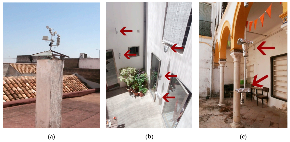
Simultaneously, the temperatures in the courtyards of the selected case studies were recorded with sensors’ model TESTO 174 H and TESTO 174 T, whose technical data are shown in Table 2. The sensors were placed vertically suspended from the roof of the building on the north-facing façade of the courtyard so that solar radiation would not influence the results. In addition, they were protected with a reflective shield to prevent overheating and to allow ventilation of the measuring equipment (Figure 1). As the sensors’ measured temperature would vary throughout the courtyard due to several factors, including stratification and infrared radiation, all the sensors were placed at +1.00 m and +2.00 m, referring to the height of the courtyard inhabited by users.

2.3. Problem Setup

In this article, the variables selected to predict the value of the temperature inside a courtyard are the two most relevant according to the literature review, namely, TR—considering climate location zone and year´s season, and AR—as a numerical parameter synthesizing courtyard geometry. To perform the modeling, two stages were considered.

In the first stage, work was accomplished with the data from 22 monitored courtyards in every hour of one week, from different periods of the year, in various courtyards located in the Spanish cities of Badajoz, Córdoba and Seville.

The SVM method was used to create the library with some of these training data along one week in different courtyards. After that, we consider courtyards with different characteristic parameters, such as ARI and ARII, which are not included in the training data and use interpolation techniques to obtain the prediction for a week.

2.4. Support Vector Regression Method

Support Vector Machines (SVMs) were introduced in the 90s by Vapnik and his collaborators [45] in the framework of statistical learning theory. Although originally, SVMs were thought to solve binary classification problems, they are currently used to solve various types of problems, for example, regression problems [44], on which this research has focused.

In this first stage, the predicted value of the measured temperature inside a courtyard using some information related to it has been obtained. In particular, the time (hour of the day), the outside CMT, the wind speed and direction have been considered. More specifically, the following has been considered: $x=\left(x^1,x^2,x^3,x^4\right),$ where,

• $x^1$ = time (hour of the day);
• $x^2$ = outside temperature;
• $x^3$ = wind speed;
• $x^4$ = wind direction.

Searching for a function $f:R^4\to \mathrm{R}$, such that $y=f\left(x\right)$ provides the temperature inside the courtyard was the goal in this step.

To find this function $f$ for each courtyard, the $m$-collection of experimental data associated with it was used. The idea of the SVR method [6] is to obtain a function such that for every sample $\left(x_i,y_i\right)$, $i=1,\dots ,m$, it is satisfied that $\left|f\left(x_i\right)-y_i\right| \le \epsilon ,$ for some $\epsilon >0$ small. Concretely, given $\epsilon ,\gamma$ and $C>0$, the following optimization problem is considered:

$$\underset{}{\max }\left\{-\frac{1}{2}\sum _{i,j=1}^m\left({\alpha }_i-{\alpha }_i^{\ast }\right)\left({\alpha }_j-{\alpha }_j^{\ast }\right)\exp \left(-\mathsf{\gamma }\parallel x_i-x_j{\parallel }^2\right) - \epsilon \sum _{i,j=1}^m\left({\alpha }_i+{\alpha }_i^{\ast }\right)+\sum _{i,j=1}^m{y}_i\left({\alpha }_i-{\alpha }_i^{\ast }\right)\right\},$$

$$\mathrm{subject} \mathrm{to} \begin{array}{c}{\sum }_{i,j=1}^m({\alpha }_i-{\alpha }_i^{\ast })=0,\hspace{1em} \mathrm{for} {\alpha }_i,{\alpha }_i^{\ast }\in \left[0,C\right].\end{array}$$

This problem was solved using the statistical software $R$. In particular, we used the E1071 library [52], a software package designed to solve classification and regression problems, using Support Vector Machines, which can be easily installed in $R$. The solution provides a possible candidate function as follows:

$$f\left(x\right)={\displaystyle \sum }_{i=1}^m({\alpha }_i-{\alpha }_i^{\ast })\exp \left(-\gamma \parallel x_i-x{\parallel }^2\right)+b,$$

where the constant $b \in R$ can be computed by forcing the Karush–Kuhn–Tucker (KKT) condition [53]. The function $K\left(x,x^{\prime }\right)=\exp \left(-\gamma \parallel x-x^{\prime }{\parallel }^2\right)$ is called the radial basis kernel. It holds that $\left|f\left(x_i\right)-y_i\right|\le \epsilon ,$ for all $i=1,\dots ,m$. The quality of function $f$ depends on the choice of the parameters $\epsilon ,\gamma$ and $C$. In order to select the best parameters, Cross-Validation (CV) technique was used to obtain the parameter values: γ = 0.1, C = 10 and ε = 0.1, with a CV error around 1% for all test cases.

2.5. Predicted Temperature of a Courtyard

In the first stage, through the monitoring data and the SVR method, a library of predicted temperatures inside various courtyards located in different cities of the south of Spain was obtained. In this second stage, by using this library, the predicted temperature inside a given courtyard was obtained.

In this section, given that the definition of AR is two-dimensional, two ARs were measured: the first one, ARI was defined as the relation between the width and the height, and the second one, ARII was defined as the relation between the length and the height, as follows:

$$\mathrm{ARI}=h_{max}/W\hspace{1em}\mathrm{and}\hspace{1em}\mathrm{ARII}=h_{max}/L,$$

where $h_{max}$ is the maximum height, $W$ represents the width and $L$ the length of the courtyard.

Once both ARs were fixed, the predicted temperature inside a given courtyard in two different ways was performed. First, the courtyards library was classified considering three different TRs, depending on the range of temperatures of the courtyards and an interpolation technique to predict the temperature inside a courtyard of the same class by using ARs data was used, as it is explained in Section 2.5.1.

Second, the courtyards library was classified into different groups, depending on the courtyards AR range and an interpolation technique to predict the temperature inside a courtyard of the same class by using the maximum and minimum temperature data was used. Two cases (AR.1 and AR.2) were considered: first, the classification by considering ARI, and second, ARII was performed.

2.5.1. Fixed Temperature Range, Interpolation Using the ARs

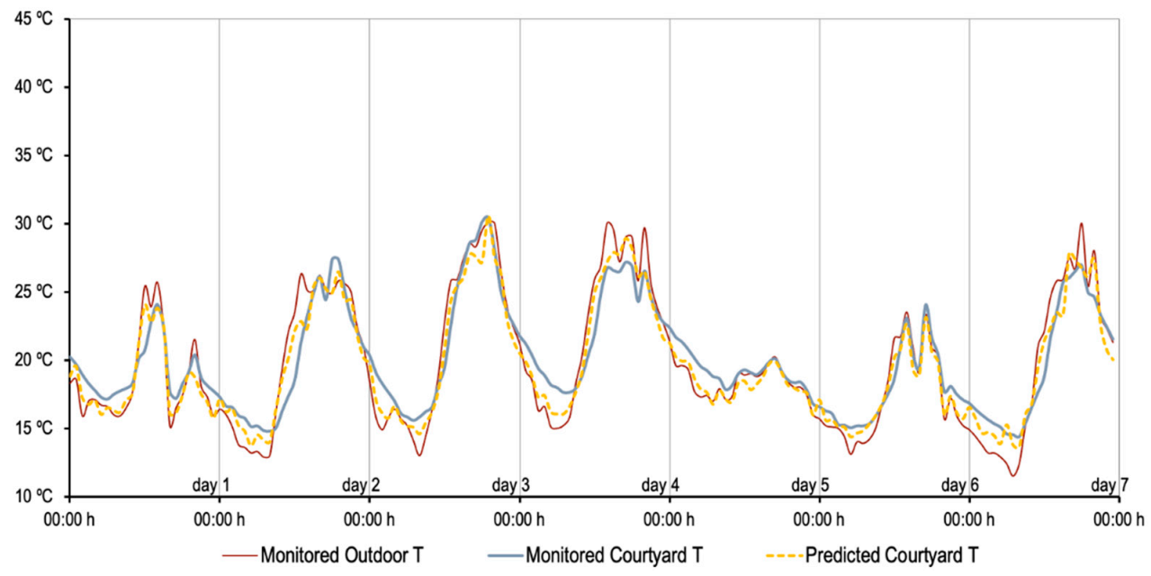
In this case, the courtyards library was classified into three different TR, depending on the range of temperatures inside the courtyard. These TRs correspond to statistical climatic records in the locations where case studies are placed. The first group corresponds to the hottest days of spring or autumn, the second, to a typical summer season and, the third, to a summer heatwave.

TR1: $\left({15}^{\circ },{35}^{\circ }\right)$.

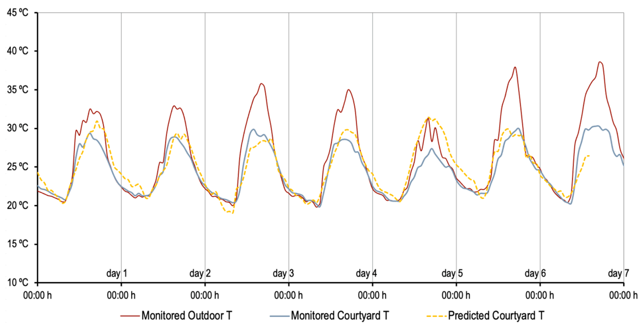
TR2: $\left({20}^{\circ },{40}^{\circ }\right)$.

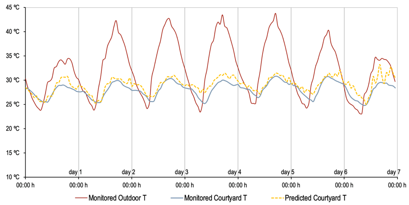
TR3: $\left({25}^{\circ },{45}^{\circ }\right)$.

In the following

Table 3. Classification of courtyards within temperature range classes.

Thermal Range	Courtyards
TR1	CS1, CS2, CS3, CS4
TR2	CS5, CS6, CS7, CS8, CS9, CS10, CS11, CS12, CS13, CS14
TR3	CS16, CS17, CS18, CS19, CS20, CS21, CS22

, the courtyards are classified within these different TR. Note that some courtyards are in more than one TR because the temperature range in the courtyard changed from one week to another. This is because the courtyard, as a thermal tempering device, performs differently depending on the outdoor temperature.

For a given courtyard, its range of temperature is first estimated, being classified as TR1, TR2 or TR3, and its AR, being classified as ARI or ARII.

Once courtyards are classified, the temperature prediction is verified through the SVR method; by an interpolation technique, it can be obtained a prediction of the temperature inside a courtyard of the same class. To achieve these data, MATLAB function scatteredInterpolant was used, which performs interpolation on a 2D dataset of scattered data. In particular, it returns the interpolant $F$ for the given dataset such that we can evaluate $F$ at a set of query points in 2D to produce interpolated values T_q = F (ARI_q, ARII_q), obtaining the temperature inside the courtyard $T_q$.

2.5.2. Fixed the ARs, Interpolation Using Minimum and Maximum Temperatures

In this section, two different cases, depending on whether we fix ARI or ARII, are considered.

First, the courtyards library was classified into two different classes, depending on $ARI$:

ARI.1: $\left(0,1\right)$.

ARI.2: $\left(1,2\right)$.

In the following

Table 4. Classification of courtyards within ARI range class.

ARI Range Class	Courtyards
ARI.1	CS5, CS8, CS11, CS13, CS14, CS15, CS16, CS19, CS22
ARI.2	CS1, CS2, CS3, CS6, CS7, CS9, CS10, CS12, CS17, CS18, CS20, CS21

, the courtyards are classified within these different classes. Note that CS4 has not been taken into account, as its ARI is out of the considered ranges (3.41).

Thus, for a given courtyard, we measure the ARI and classify it into ARI.1 or ARI.2.

Then, given the minimum and maximum temperature, $T_{min}$ and $T_{max}$, respectively, of some courtyards in the same class and their corresponding predicted temperatures through the SVR method, by an interpolation technique implemented in the scientific software MATLAB, it can be obtained a prediction of the temperature inside a courtyard of the same class. To do the interpolation, we have used again the MATLAB function scatteredInterpolant, which performs interpolation on a 2D dataset of scattered data. In this case, we obtained $T_q=F\left(T_{min,q},T_{max,q}\right),$ obtaining the temperature inside the courtyard $T_q$.

Second, we classified the courtyards library into two different classes, depending on $ARII$:

ARII.1: $\left(0,1\right)$.

ARII.2: $\left(1,2.5\right)$.

In the following

Table 5. Classification of courtyards within ARII range class.

ARII Range Class	Courtyards
ARII.1	CS1, CS3, CS4, CS5, CS8, CS11, CS14, CS16, CS19, CS22
ARII.2	CS2, CS6, CS7, CS9, CS10, CS12, CS13, CS15, CS17, CS18, CS20, CS21

, we classify the courtyards within these different classes:

Thus, for a given courtyard, first it was measured the ARII, being classified as ARII.1 or as ARII.2. To do the interpolation, the same procedure as in the case of ARI was followed, using now ARII instead.

3. Results

3.1. Fixed Temperature Range, Interpolation Using AR

In this section, it is shown the predicted temperature obtained by the method proposed in Section 2.5.1 in one courtyard of each temperature range class. The predicted temperature in comparison to the monitored temperature inside the courtyard, as well as the outdoor temperature, are both represented. In addition, a quantitative analysis was carried out. On the one hand, it was evaluated the relative error of the predicted temperature with respect to the monitored temperature in different discrete norms:

$$\begin{gathered} L^1\hspace{0.17em}\left(\%\right)=\frac{{{\displaystyle \sum }}_{i=1}^N|T_{monit.}-T_{pred.}|\left(t_i\right)}{{{\displaystyle \sum }}_{i=1}^N{T}_{monit.}\left(t_i\right)}\cdot 100, \\ {L}^2\hspace{0.17em}\left(\%\right)={\left[\frac{{{\displaystyle \sum }}_{i=1}^N{(T_{monit.}-T_{pred.})}^2\left(t_i\right)}{{{\displaystyle \sum }}_{i=1}^N{T}_{monit.}^2\left(t_i\right)}\right]}^{1/2}\cdot 100, \end{gathered}$$

where it is denoted by $T_{monit.}\left(t_i\right)$ (resp, $T_{pred.}\left(t_i\right)$), the monitored temperature (resp., the predicted temperature) at time $t_i,i=1,\dots ,N$ (hours, (h)). Moreover, the percentage in time for which the obtained absolute error within the predicted and the monitored temperature is less than or equal to a fixed tolerance $tol=2^{ \circ }\mathrm{C}$ was evaluated. On the other hand, the following statistical parameters were computed: the correlation coefficient $R$, the Root Mean Square Error ($RMSE$) and the Mean Absolute Percentage Error ($MAPE$). The formulas for these parameters are as follows:

$$R=\frac{{{\displaystyle \sum }}_{i=1}^N(T_{monit.}\left(t_i\right)-{\overline{T}}_{monit.})\left(T_{pred.}\left(t_i\right)-{\overline{T}}_{pred.}\right)}{{\left[{\displaystyle \sum _{i=1}^N}{(T_{monit.}\left(t_i\right)-{\overline{T}}_{monit.})}^2{\displaystyle \sum _{i=1}^N}{(T_{pred.}\left(t_i\right)-{\overline{T}}_{pred.})}^2\right]}^{1/2}},$$

$$RMSE\hspace{0.17em}{(}^{o}C)={\left[\frac{{{\displaystyle \sum }}_{i=1}^N{(T_{monit.}-T_{pred.})}^2\left(t_i\right)}{N}\right]}^{1/2},$$

$$MAPE\hspace{0.17em}\left(\%\right)=\frac{1}{N}{{\displaystyle \sum }}_{i=1}^N\frac{\left|T_{monit.}-T_{pred.}\right|\left(t_i\right)}{T_{monit.}\left(t_i\right)}\cdot 100,$$

where, in the formula for the correlation coefficient $R,$ the mean monitored temperature (resp., the mean predicted temperature) is denoted by ${\overline{T}}_{monit.}$ (resp, ${\overline{T}}_{pred.}$). The values of the relative and absolute errors and the statistical parameters are shown in

Table 6. Example 3.0.1. Relative and absolute errors for the courtyard measured temperature in each selected courtyard of each TR.

Thermal Range	${\mathit{L}}^{\mathbf{1}}$ (%)	${\mathit{L}}^{\mathbf{2}}$ (%)	Absolute Error  $\mathbf{\le }\mathit{tol}$ (%)
TR1	$5.09$	$6.10$	$91.67$
TR2	$4.93$	$6.62$	$84.28$
TR3	$3.50$	$4.31$	$89.88$

and

Table 7. Example 3.0.1. Statistical parameters for the courtyard measured temperature in each selected courtyard of each TR.

Thermal Range	$\mathit{R}$	RMSE (°C)	MAPE (%)
TR1	$0.96$	$1.24$	$5.17$
TR2	$0.88$	$1.62$	$4.82$
TR3	$0.89$	$1.21$	$3.52$

for the CMT in each selected courtyard of each temperature range class.

For the class TR1, the courtyard CS1, located in Badajoz was considered. The prediction is performed for the dates 20 to 26 May. In the graph (Figure 2), simulation versus monitoring results of this courtyard with mild and very irregular temperatures is shown. There is hardly any thermal gap, and the prediction shows good accuracy. The obtained results are specified in Table 6 and Table 7 (first row).

For the class TR2, the courtyard CS5, located in Seville, was considered. The prediction is performed for the date 7 to 13 September. The obtained results are represented in Figure 3 and Table 6 and Table 7 (second row). Note that the prediction for the second half of the last day is not represented in this plot. This is due to the fact that some of the training data used for this prediction had fewer points than the 168 needed for the whole week. However, to be consistent with the other cases, we decided to keep the whole week in this plot.

For the class TR3, the courtyard CS17, located in Córdoba, was considered. The prediction is performed for the date 26 July to 1 August. Unlike the previous case shown in Figure 2, in this one (Figure 4), the outside temperature is higher and there is a large thermal gap. The predicted results show similarly good accuracy, particularly on days of maximum outdoor temperature. The obtained results are detailed in Table 6 and Table 7 (third row).

3.2. Fixed AR, Interpolation Using Minimum and Maximum Temperature

In this section, the predicted temperature obtained by the method proposed in Section 2.5.2 in one courtyard of each AR range class is shown. First, the ARI range class is considered, representing the predicted temperature in comparison to the monitored temperature inside the courtyard, as well as the outdoor temperature. Additionally, a quantitative analysis was carried out. On the one hand, the relative error of the predicted temperature with respect to the monitored temperature in different discrete norms ($L^1$ and $L^2$) was evaluated, as done in Section 3.1. Moreover, the percentage in time for which the obtained absolute error within the predicted and the monitored temperature is less than or equal to a fixed tolerance $tol=2^{ \circ }\mathrm{C}$ was also evaluated. On the other hand, the following statistical parameters were computed: $R$, $RMSE$ and $MAPE$. The values of the relative and absolute errors and the statistical parameters are shown in

Table 8. Example 3.0.1. Statistical parameters for the courtyard measured temperature in each selected courtyard of each temperature range class.

$\mathit{ARI}$ Range Class	${\mathit{L}}^{\mathbf{1}}$ (%)	${\mathit{L}}^{\mathbf{2}}$ (%)	Absolute Error  $\mathbf{\le }\mathit{tol}$ (%)
ARI.1	$5.79$	$7.05$	$61.45$
ARI.2	$5.09$	$6.10$	$91.67$

and

Table 9. Example 3.0.2. Statistical parameters for the courtyard measured temperature in each selected courtyard of each ARI range class.

$\mathit{ARI}$ Range Class	$\mathit{R}$	RMSE (°C)	MAPE (%)
ARI.1	$0.92$	$2.30$	$5.99$
ARI.2	$0.96$	$1.24$	$5.17$

for the courtyard measured temperature in each selected courtyard of each ARI range class.

For the ARI.1, the courtyard CS16, located in Córdoba, was considered. The prediction is performed for the date 26 July to 1 August. The obtained results are represented in Figure 5 and Table 7 and Table 8 (first row).

For the class ARI.2, the courtyard CS1, located in Badajoz, was considered. The prediction is performed for the date 20 to 26 May. The obtained results are represented in Figure 6 and Table 7 and Table 8 (second row).

Finally, the ARII range class was considered and the predicted temperature was represented in comparison to the monitored temperature inside the courtyard as well as the outdoor temperature. As before, a quantitative analysis was carried out. On the one hand, the relative error of the predicted temperature with respect to the monitored temperature in different discrete norms ($L^1$ and $L^2$) was evaluated, as done in Section 3.1. Moreover, the percentage in time for which the obtained absolute error within the predicted and the monitored temperature is less than or equal to a fixed tolerance $tol=2^{ \circ }\mathrm{C}$ was also evaluated. On the other hand, the following statistical parameters were computed: $R$, $RMSE$ and $MAPE$. The values of the relative and absolute errors, and the statistical parameters are shown in in

Table 10. Example 3.0.2. Relative and absolute errors for the courtyard measured temperature in each selected courtyard of each ARII range class.

$\mathit{ARII}$ Range Class	${\mathit{L}}^{\mathbf{1}}$ (%)	${\mathit{L}}^{\mathbf{2}}$ (%)	Absolute Error  $\mathbf{\le }\mathit{tol}$ (%)
ARII.1	$10.10$	$12.69$	$58.33$
ARII.2	$4.80$	$5.87$	$80.72$

and

Table 11. Example 3.0.2. Statistical parameters for the courtyard measured temperature in each selected courtyard of each ARII range class.

$\mathit{ARII}$ Range Class	$\mathit{R}$	RMSE (°C)	MAPE (%)
ARII.1	$0.64$	$2.65$	$9.78$
ARII.2	$0.79$	$1.46$	$4.86$

for the courtyard measured temperature in each selected courtyard of each ARII range class.

For the class ARII.1, the courtyard CS4, located in Badajoz, was considered. The prediction is performed for the date 20 to 26 May. In this case, as can be seen in Figure 7, the courtyard has a different thermal performance than in the previously described case studies. This is mainly due to the overheating that occurs in the early morning hours due to the low AR. The predicted results do not show such a tight accuracy under these conditions. The obtained results are detailed in Table 9 and Table 10 (first row).

For the class ARII.2, the courtyard CS9, located in Seville, was considered. The prediction is performed for the date 4 to 10 September. The obtained results are represented in Figure 8 and Table 9 and Table 10 (second row).

3.3. Relative Errors Calculation

The main goal of this work is the accurate thermal modeling of the courtyard for its optimization as a resilient strategy against climate change and urban overheating. Therefore, the specific performance of courtyard thermodynamics was considered for the evaluation of the model errors. The courtyard´s thermal tempering performance increases as a function of the Thermal Gap (from now on, TG), that is, the difference between the exterior monitored temperature and the monitored temperature inside the courtyard. TG usually increases as the outside temperature rises. Accordingly, in this section, relative errors from two different and representative case studies with different TRs are selected, comparing statistical parameters more in detail.

The first selected case study corresponds to the predicted temperature inside the TR1 courtyard CS1 (Figure 2), and the second case corresponds to the predicted temperature inside the TR3 courtyard CS17 (Figure 4). These cases were selected since, in the first case, monitored and predicted temperatures inside the courtyard are rather close to the exterior monitored one, while in the second case, monitored and predicted temperatures inside the courtyard are quite far from the exterior monitored one.

Conversely, the relative and absolute errors, as well as the statistical parameters considered in the previous section, were computed. Then, the daily computations all along the week were performed. The obtained results are given in

Table 12. Relative error CS1.

Errors + Stat. Param.\Day	1	2	3	4	5	6	7
$L^1\hspace{0.17em}\left(\%\right)$	5.70	5.55	4.77	5.67	4.57	3.62	5.55
$L^2\hspace{0.17em}\left(\%\right)$	6.79	6.95	5.62	6.40	5.30	4.42	6.52
Absolute error $\le tol\hspace{0.17em}\left(\%\right)$	95.83	83.33	87.50	91.67	95.83	100	87.50
$R$	0.92	0.95	0.98	0.97	0.91	0.97	0.96
$RMSE\hspace{0.17em}{(}^{\circ }\mathrm{C})$	1.30	1.41	1.25	1.44	1.03	0.80	1.32
$MAPE\hspace{0.17em}\left(\%\right)$	5.82	5.84	4.91	5.90	4.54	3.57	5.60

and

Table 13. Relative Error CS17.

Errors + Stat. Param.\Day	1	2	3	4	5	6	7
$L^1\hspace{0.17em}\left(\%\right)$	2.16	2.68	2.71	5.10	2.40	3.23	5.95
$L^2\hspace{0.17em}\left(\%\right)$	3.26	3.14	3.03	5.48	2.65	3.92	7.02
Absolute error $\le tol\hspace{0.17em}\left(\%\right)$	95.83	95.83	100	83.33	100	95.83	58.33
$R$	0.91	0.96	0.96	0.92	0.97	0.91	0.89
$RMSE\hspace{0.17em}{(}^{\circ }\mathrm{C})$	0.90	0.87	0.85	1.54	0.76	1.12	1.93
$MAPE\hspace{0.17em}\left(\%\right)$	2.42	2.65	2.74	5.18	2.42	3.30	5.91

.

On the other hand, bearing in mind the obtained results, the best predicted day in each week was selected. In the first case, the day that gives better performances is the 6th one, while in the second case, it is the 5th one. Then, the relative error of the predicted temperature was computed hourly and represented in two ways. In the first way, with respect to the TG and in the second way, with respect to the monitored temperature. The graphics corresponding to CS1 and CS17 are included in Figure 9a,b, respectively. The graphic represented in Figure 9a corresponds to the relative error of the predicted temperature with respect to TG, and the graphic in Figure 9b corresponds to the relative error of the predicted temperature with respect to the monitored temperature inside the courtyard. In addition, the segment of the day in which critical urban overheating is concentrated is indicated in each graph. These hours, according to climate records [54], are between 13:00 and 19:00. On the left, considering CS1 plotted in Figure 9a, it can be observed that the relative error with respect to TG is always below 3%, except for two peaks, corresponding to time slots where the exterior temperature and the monitored temperature inside the courtyard almost coincide. Considering CS17 in Figure 9a, it was obtained a very low relative error with respect to TG in the central time slot of the day, that is, between 13:00 and 19:00, where TG is large. On the right, regarding the relative error with respect to the courtyard measured temperature (CMT) in Figure 9b, it can be observed that the plotted relative error for CS1 is below 0.1%, while for CS17, this relative error is always below 0.05%. For both case studies, if the daytime slot with the highest urban overheating is considered, the relative error is always below 0.05%.

4. Discussion

In this section, the results that were obtained in Section 3 are discussed. Regarding the results obtained in Section 3.1 and Section 3.2, on the one hand, it can be appreciated in Table 6, Table 8 and Table 10 that the values for the relative errors in different discrete norms are around 5% and in almost all cases are below 10%, and the percentage in time for which the obtained absolute error w.r.t. the CMT is less than or equal to $tol=2^{ \circ }\mathrm{C}$ is superior to 80%, except for the cases of Example 3.0.2, the ARI.1 range class and the ARII.1 range class. For the first critical case, reasonable values for the relative errors in different discrete norms (within 5% and 8%) were obtained, and the percentage in time for which the obtained absolute error w.r.t. the CMT is less than or equal to $tol=2^{ \circ }\mathrm{C}$ is 61.45%. However, that case is rather special since it can be observed at relatively high temperatures w.r.t. the other experiments. In any case, if the tolerance parameter is increased to $tol=3{ }^{\circ }\mathrm{C}$ for that case, a higher percentage of up to 80.72%, can be obtained. For the second critical case, the relative errors in different discrete norms are within 10% and 13%, and the percentage in time for which the obtained absolute error w.r.t. the CMT is less than or equal to $tol=2{ }^{\circ }\mathrm{C}$ is 58.33%. In any case, if the tolerance parameter is increased to $tol=3^{ \circ }\mathrm{C}$ for that case, we obtain the higher percentage 74.40%. On the other hand, the values for the statistical parameters that indicate that the simulation is accurate are $R\to 1$, $RMSE\to 0$, $MAPE\to 0$ [36,42,43,44,50,51,52]. The values of these parameters for the courtyard measured temperature in the present courtyards for each simulation confirm that the used strategy is rather accurate. In particular, in Table 7, Table 9 and Table 11 it can be observed that the correlation coefficient $R$ is quite close to 1 for all range classes (superior to 0.85, except for the cases Example 3.0.2 ARII.1 and ARII.2 range classes for which it is within 0.6 and 0.8). The $RMSE$ values are around $1.5{ }^{\circ }\hspace{0.17em}\mathrm{C}$ and the $MAPE$ values are around 5%, except for the critical cases identified above for which the $RMSE$ values are around ${2.5}^{ \circ }\mathrm{C}$ and the $MAPE$ values are within 5% and 10%.

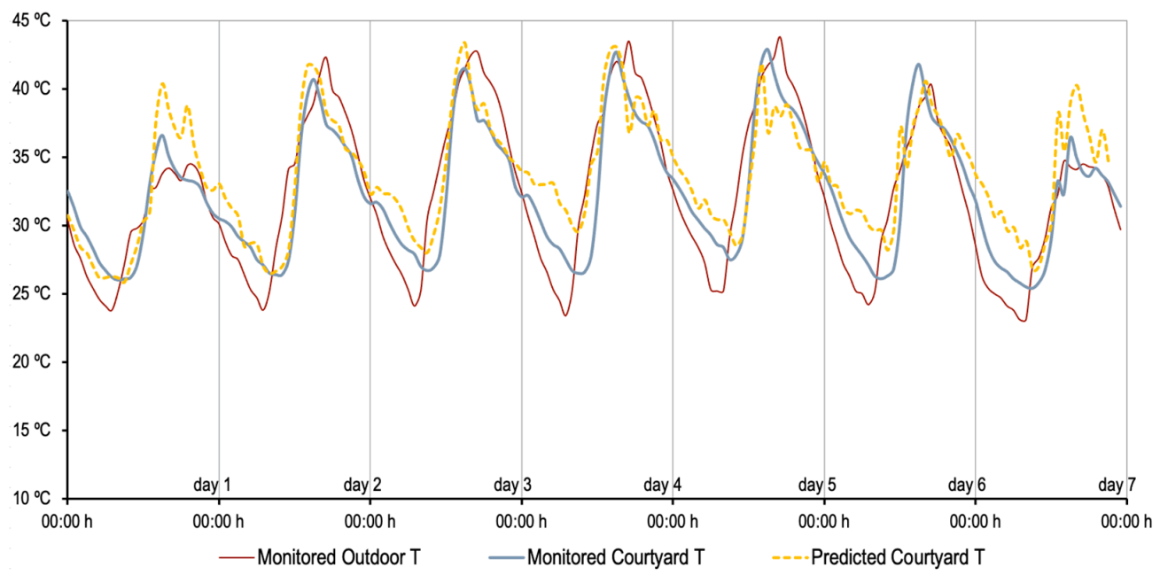
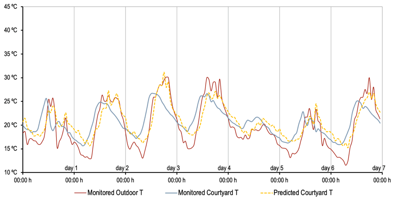
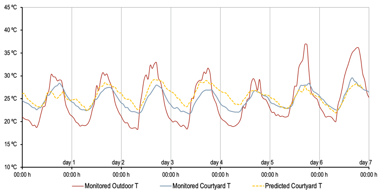
Finally, in Section 3.3, relative and absolute errors as well as the statistical parameters in two selected cases were computed daily. The case where the predicted CMT inside the courtyard is rather close to the exterior one, and the case where the predicted CMT inside the courtyard is quite far from the exterior one were chosen. The obtained results are given in Table 12 and Table 13, respectively. It can be observed that the values for the relative errors in different discrete norms are around 6% in the first case, and around 3% in the second case, and in almost all cases are below 7%. Moreover, the percentage in time for which the obtained absolute error w.r.t. the CMT is less than or equal to $tol=2{ }^{\circ }\mathrm{C}$ is superior to 80% all the days except for the 7th day of the second case, arriving to 100% in the 6th day of the first case and on the 3rd and 5th day of the second case. With respect to statistical parameters, the correlation coefficient R is quite close to 1, being larger than 0.89 in all cases. The $RMSE$ values are around $1.25{ }^{\circ }\mathrm{C}$ in the first case and $1^{ \circ }\mathrm{C}$ in the second one, and the $MAPE$ values are around 5% in the first case and 3% in the second case. Thus, mostly, the results obtained in Section 3.3 daily in these selected cases improve the global results computed for the whole week in Section 3.1 and Section 3.2.

In brief, apart from the critical cases identified above, the values of the statistical parameters considered are in a similar range than those obtained in [36] for a similar problem. In that work, the authors performed a very accurate courtyard thermal simulation based upon a Computational Fluid Dynamics (CFD) FreeFEM 3D model, which is much more computationally expensive than the ML technique SVR used in this work. In particular, the computation of one-week temperature through the SVR method takes around one minute, while the CFD method takes around four minutes per one day of simulation.

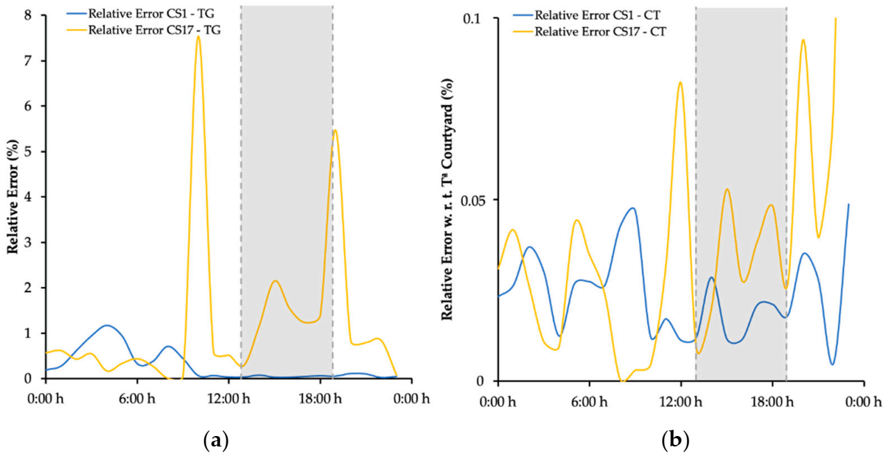
5. Conclusions

In the present work, the applicability of a supervised ML model as a suitable tool for predicting microclimatic performance inside courtyards has been evaluated. For this purpose, among the ML models developed as supervised learning, Support Vector Machines (SVM) were selected. The model was fed and validated with empirical data from 22 case studies in southern Spain.

The results provided by this strategy showed good accuracy when compared to monitored data. In particular, we selected two representative and highly meaningful case studies with different TGs. The final results for both cases showed that, when the daytime slot with the highest urban overheating is considered, the relative error is almost below 0.05%. Additionally, values for statistical parameters are in good agreement with other studies in the literature that use more computationally expensive CFD models and show more accuracy than existing commercial tools. Indeed, the present strategy shows a Root Mean Square Error (RMSE) around $1{ }^{\circ }\mathrm{C}$ for the two representative case studies selected, which is in a similar range to the values obtained in [36] for a similar problem by a more computationally expensive CFD model, while corresponding values for existing commercial software are typically around $3{ }^{\circ }\mathrm{C}$.

Based on the results obtained, it can be stated that the new application proposed for the ML method is useful for the development of design and measurement tools capable of modeling the complex microclimate of courtyards. Furthermore, the accuracy of the predictions for the analyzed case studies increases as a function of the courtyard thermal tempering potential linked to the intensification of the outdoor temperature.

The enhancement of the proposed methodology with the inclusion of other complementary microclimatic strategies, such as shading devices or vegetation as new ML features as well as establishing a balance between an over fitted and under fitted ML model considering the optimal number of training data, can be considered as future ways to develop this research.