A New Class of Estimators Based on a General Relative Loss Function

Abstract

Motivated by the relative loss estimator of the median, we propose a new class of estimators for linear quantile models using a general relative loss function defined by the Box–Cox transformation function. The proposed method is very flexible. It includes a traditional quantile regression and median regression under the relative loss as special cases. Compared to the traditional linear quantile estimator, the proposed estimator has smaller variance and hence is more efficient in making statistical inferences. We show that, in theory, the proposed estimator is consistent and asymptotically normal under appropriate conditions. Extensive simulation studies were conducted, demonstrating good performance of the proposed method. An application of the proposed method in a prostate cancer study is provided.

1. Introduction

In contrast to the mean-based regression that mainly gives an overall quantification for the central covariate effect, quantile regression can directly model a series of quantiles (from lower to higher) of the response variable to deliver a global evaluation of the covariate effect [1,2]. A major advantage of quantile regression is that no assumptions about the distribution of the response are required, which makes it practical, robust and amenable to skewed response distributions [3]. Additionally, quantile regression methods can help to handle the cases of heteroscedasticity [4]. Nowadays, quantile regressions have been widely used in many fields, established numerous methodologies covering linear, nonlinear and longitudinal quantile regressions [5,6], as well as applications in survival analysis [7]. Application studies show that quantile regression allows adjustment for potential confounders and calculation of interaction terms and variable selection, while being more robust to statistical outliers and yielding much more information about the underlying associations [1,3]. However, the computation of quantile regressions is relatively complex and somewhat unique, especially compared with ordinary least squares for mean-based linear (or nonlinear) regressions. Take a 0.5 quantile estimation as an example: the quantile regression minimizes the sum of weighted absolute residuals instead of squared residuals [8]. One drawback of quantile regressions is that the estimation efficiency fluctuates a lot at different quantiles and is relatively low at the tails [9]. A traditional quantile regression is typically based on minimizing a check loss function [1], but often the relative quantile loss could be more relevant than the check loss function and hence might be used to gain more efficiency for inference. So far, to the best of our knowledge, there have been no consistent studies on other type of loss functions, such as the relative error loss for quantile regression.

In many practical applications, the magnitude of the relative error, rather than the absolute error, is of the major concern. In general, the relative error is more relevant when the range of predicted values is large and that of predictors is small. Narula and Wellington (1977) proposed an estimation approach for linear models by minimizing the sum of relative errors [10], without any theoretical results. Khoshgoftaar et al. (1992) studied the asymptotic properties of the estimators by minimizing both the squared relative loss and the absolute relative loss under nonlinear regression models [11], and made a great comparative study on them. Later, Chen et al. (2010) applied the least absolute relative error loss [12] for the linear regression model

$$Y_i^{*}=X_i^T\beta +{\epsilon }_i^{*},$$

and proposed to estimate the model parameters by minimizing the sum of the absolute relative error

$$\sum _{i=1}^n\left\{\left|\frac{Y_i-exp\left(X_i^T\beta \right)}{Y_i}\right|+\left|\frac{Y_i-exp\left(X_i^T\beta \right)}{exp\left(X_i^T\beta \right)}\right|\right\},$$

where $Y_i=log\left(Y_i^{*}\right)$ and they assumed $log\left({\epsilon }_i^{*}\right)$ has a mean of 1. Motivated by [12], Yang and Ye (2013) established the connection between relative error estimators and the M-estimation under a linear model [13]. However, their works only consider the absolute relative loss, not related to any quantile estimates of model distribution. None of these studies discussed the way to apply the relative error for a general quantile regression.

In this article, we propose a general class of relative loss functions via a Box–Cox transformation [14,15]. The proposed loss function includes the absolute loss and the relative loss as special cases. We also show that the proposed loss function is convex, scale-free and able to be elicited. We apply the proposed loss function for a linear quantile regression [1] and prove that the estimates of the regression coefficients are consistent and asymptotically normal. Through numerical studies on two concrete examples that have well-derived theoretical solutions, we show that the proposed method is feasible and verify that the numerical results have the expected theoretical properties obtained from the theoretical study. We also apply the proposed method to a prostate cancer study, showing that our method provides more accurate statistical inferences on quantile estimates compared to the regular quantile regression, especially at the region of tail quantiles.

The rest of this article is organized as follows. In Section 2, we introduce the model and propose the estimation procedure. In Section 3, we establish the consistency and asymptotic normality for the parameter estimates under certain regularity conditions. In Section 4, we examine the finite-sample properties using two simple simulations. An application example is given in Section 5 with a prostate cancer study. We conclude with a brief summary and remarks in Section 6.

2. Model and Methods

Let $Y_i$ be the response of interest and $X_i$ be a $(p+1)$-dimensional covariate with the first element being 1. Consider a linear quantile regression model

$$Y_i=X_i^T{\beta }_0\left(\tau \right)+{ϵ}_i\left(\tau \right),i=1,\dots ,n,$$

(1)

where ${\beta }_0\left(\tau \right)$ is a $(p+1)$-dimensional coefficient for some $\tau \in (0,1)$, and ${ϵ}_i\left(\tau \right)$ is a random error with the $\tau$th quantile being equal to 0 conditional on $X_i$. In model (1), $Y_i$ could also be replaced by any other reasonable monotone transformation, but considering that a linear relationship in the transformed model may not be linear in the original scale, one may need to transform the result back to the original measurement scale for the interpretation.

Through an exponential transformation, model (1) can be rewritten as

$$T_i=exp\left\{X_i^T{\beta }_0\left(\tau \right)\right\}{\epsilon }_i\left(\tau \right),i=1,\dots ,n,$$

(2)

where $T_i=exp\left(Y_i\right)>0$, ${\epsilon }_i\left(\tau \right)=exp\left\{{ϵ}_i\left(\tau \right)\right\}=exp\{Y_i-X_i^T{\beta }_0\left(\tau \right)\}$. Denote $H(·)$ as a monotone function of real value, then according to the equivariance property of quantiles, $Q_{\tau }\left\{H\left({\epsilon }_i\right)\right|X_i\}=H\left\{Q_{\tau }\left({\epsilon }_i\right|X_i)\right\}$ holds for any random error ${\epsilon }_i$. Here, $Q_{\tau }\left(\epsilon \right|X)$ is the $\tau$th conditional quantile of $\epsilon$ given X. This characteristic enables us to consider quantile regressions under a proper transformation of the random error so as to enhance the estimation efficiency.

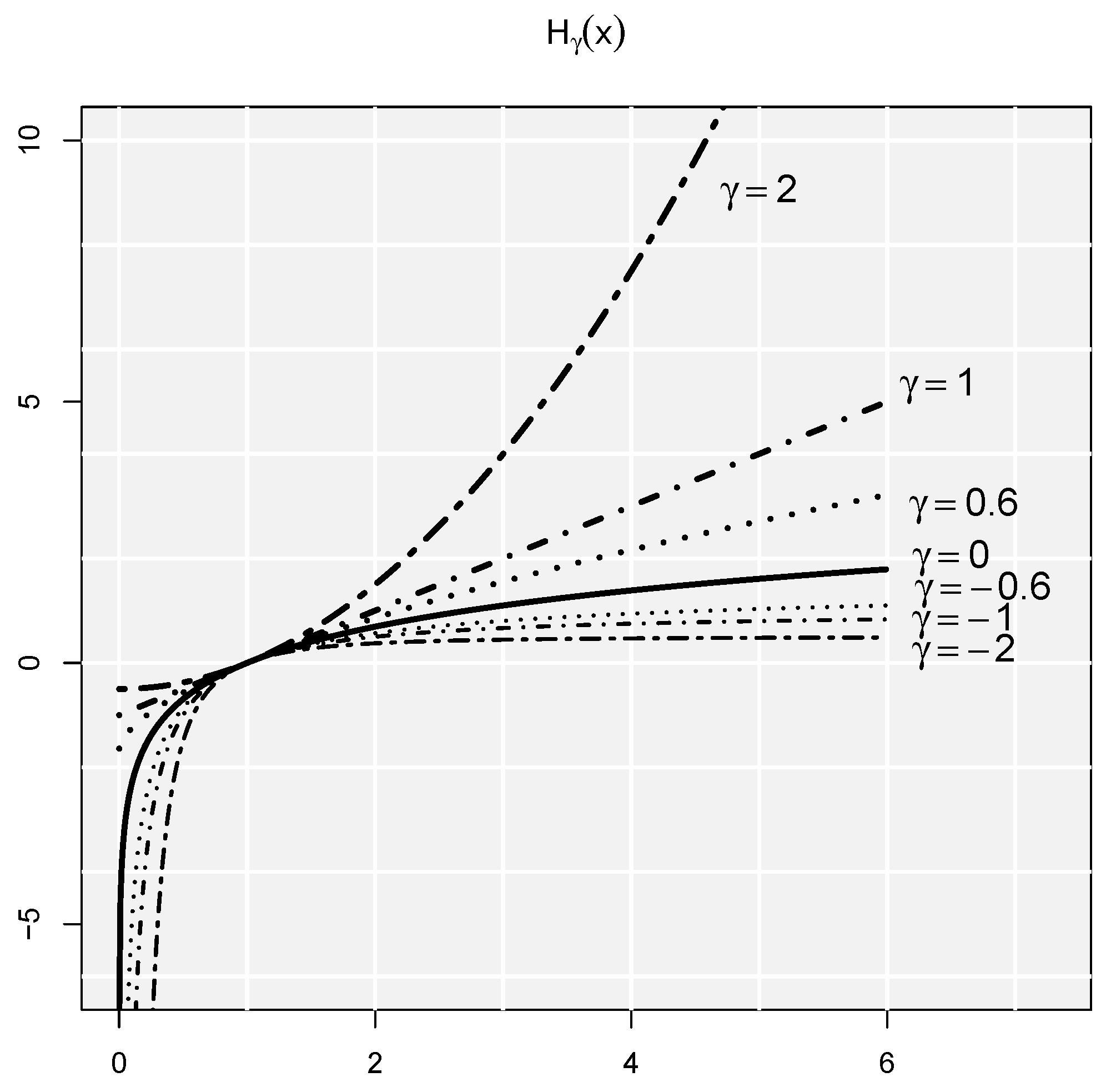
To this end, we propose to conduct the model regression using a general class of relative loss functions, which leads to the objective function in the form

$$\frac{1}{n}\sum _{i=1}^n\left\{{\rho }_{\tau }\left[H_{\gamma }\left\{T_{i}exp(-X_i^T\beta )\right\}\right]+{\rho }_{\tau }\left[H_{-\gamma }\left\{T_{i}exp(-X_i^T\beta )\right\}\right]\right\},$$

(3)

where ${\rho }_{\tau }\left(u\right)=u\{\tau -I(u<0)\}$ is the traditional quantile loss function and $H_{\gamma }(·)$ takes the Box–Cox transformation with $H_{\gamma }\left(u\right)=(u^{\gamma }-1)/\gamma$ for $\gamma \ne 0$ and $H_{\gamma }\left(u\right)=log\left(u\right)$ for $\gamma =0$ (see Figure 1).

The objective function, (3), can be further simplified as

$$\begin{array}{c}\hfill W_n(\beta ;\gamma ,\tau )=\frac{1}{n}\sum _{i=1}^n{V}_{\gamma }\left(exp(Y_i-X_i^T\beta )\right)\left\{\tau -I(Y_i<X_i^T\beta )\right\},\end{array}$$

(4)

where $V_{\gamma }\left(u\right)=(u^{\gamma }-u^{-\gamma })/\gamma$ if $\gamma \ne 0$, otherwise $V_{\gamma }\left(u\right)=2log\left(u\right)$ is a general relative loss function. In particular, if $\gamma =0$, (4) is reduced to the objective function of traditional quantile regression, and if $\gamma =1$ and $\tau =0.5$, (4) is reduced to

$$\frac{1}{n}\sum _{i=1}^n\left\{\left|\frac{T_i-exp\left(X_i^T\beta \right)}{T_i}\right|+\left|\frac{T_i-exp\left(X_i^T\beta \right)}{exp\left(X_i^T\beta \right)}\right|\right\},$$

which is exactly the objective function of the least absolute relative error in [12].

The proposed framework is very flexible—it allows us to adapt the quantile regression to either the absolute or relative loss or somewhere in between by tuning the parameter $\gamma$. Furthermore, the function $V_{\gamma }\left(u\right)$ in (4) can guarantee the proposed criterion function to be convex (see Lemma A1), scale-free, and able to be elicited (see Definition 2 in [16]). Therefore, given $\gamma$, the minimizer of $W_n(\beta ;\gamma ,\tau )$ with respect to $\beta$, denoted as ${\widehat{\beta }}_n(\gamma ;\tau )$, can be obtained conveniently using classical algorithms, such as the Nelder–Mead simplex method recommended by Yin and Cai [17].

3. Asymptotic Properties

3.1. Conditions and Main Results

We assumed that $(Y_i,X_i,{ϵ}_i\left(\tau \right))$, $i=1,\dots ,n$, are independent. Let $F_{ϵ}$ and $F_{\epsilon }$ be the cumulative distribution functions of $ϵ$ and $\epsilon$, and $F(·|X)$ be the conditional distribution function of $\epsilon$ given X. We considered a random design for X and used $f(·|X)$ to denote the corresponding density function that is almost definitely continuous in the neighborhood of 1. To establish the asymptotic properties of the estimators under a certain metric, we imposed regularity conditions as follows:

(C1)

Covariate X is bounded and does not concentrate on any hyperplane of p dimensions.

(C2)

For any fixed $\gamma$, it holds that $E\left\{{({\epsilon }^{\gamma }+{\epsilon }^{-\gamma })}^2\right|X\}<\infty$ and $E\left[({\epsilon }^{\gamma }+{\epsilon }^{-\gamma })\{\tau -I(\epsilon <1)\}\right|X]=0$.

(C3)

If $\beta (\gamma ;\tau )=\beta ({\gamma }^{*};\tau )$ for any fixed $\tau$, then $\gamma \left(\tau \right)={\gamma }^{*}\left(\tau \right)$.

(C4)

$D=E\left(X{X}^T\right)$ is a positive definite.

Condition (C1) is regular, and condition (C2) ensures the consistency and asymptotic normality, which can be treated as a generalized version of the zero mean and zero median assumptions for the least square estimation and least absolute deviation regression methods, respectively. Condition (C3) guarantees the identifiability of the adaptive parameter and regression parameters. Condition (C4) is to ensure the asymptotic normality of the estimates of the regression coefficients, similar to the finite second moment condition for the least square estimator in linear regressions.

Theorem 1.

Under conditions (C1)–(C4), for any $\tau \in (0,1)$ and any finite $\gamma \in [0,\mathsf{\Gamma }]$, $\mathsf{\Gamma }$ is a constant

$$\parallel {\widehat{\beta }}_n(\gamma ;\tau )-{\beta }_0\left(\tau \right)\parallel \to 0$$

in probability as $n\to \infty$, where $\parallel ·\parallel$ indicates the Euclidean norm.

Proof of Theorem 1.

By the results of Lemma A1 in Appendix A, we know that $W_n(\beta ;\gamma ,\tau )$ is a convex function with respect to $\beta$. According to the Convexity Lemma [18], it holds that

$$\begin{array}{c}\hfill \underset{\beta \in \mathcal{B}}{sup}\left|W_n(\beta ;\gamma ,\tau )-E\left\{W_n(\beta ;\gamma ,\tau )\right\}\right|\to 0\end{array}$$

(5)

with the probability as $n\to +\infty$ and the function $E\left\{W_n(\beta ;\gamma ,\tau )\right\}$ is necessarily convex on $\mathcal{B}$. Through an algebraic calculation, we obtain

$$\begin{array}{ccc}& & E\{W_n(\beta ;\gamma ,\tau )-W_n({\beta }_0\left(\tau \right);\gamma ,\tau )\}\hfill \\ & =& \frac{1}{n}\sum _{i=1}^{n}E\{{\rho }_{\tau }\left(\frac{T_i^{\gamma }exp(-\gamma X_i^T\beta )-1}{\gamma }\right)+{\rho }_{\tau }\left(\frac{T_i^{-\gamma }exp\left(\gamma X_i^T\beta \right)-1}{-\gamma }\right)\hfill \\ & & -{\rho }_{\tau }\left(\frac{{\epsilon }^{\gamma }-1}{\gamma }\right)-{\rho }_{\tau }\left(\frac{{\epsilon }^{-\gamma }-1}{-\gamma }\right)\}\hfill \\ & =& \frac{1}{n}\sum _{i=1}^{n}E\left[{\rho }_{\tau }\left(\frac{T_i^{\gamma }exp(-\gamma X_i^T\beta )-1}{\gamma }\right)-{\rho }_{\tau }\left(\frac{{\epsilon }_i^{\gamma }-1}{\gamma }\right)\right]\hfill \\ & & +\frac{1}{n}\sum _{i=1}^{n}E\left[{\rho }_{\tau }\left(\frac{T_i^{-\gamma }exp\left(\gamma X_i^T\beta \right)-1}{-\gamma }\right)-{\rho }_{\tau }\left(\frac{{\epsilon }_i^{-\gamma }-1}{-\gamma }\right)\right].\hfill \end{array}$$

(6)

According to the Knight’s identity [19], it holds that

$${\rho }_{\tau }(u-v)-{\rho }_{\tau }\left(u\right)=-v\{\tau -I(u<0)\}+{\int }_0^v\{I(u\le s)-I(u\le 0)\}ds,$$

Then, by using the Knight’s identity we obtain

$$\begin{array}{ccc}& & {\rho }_{\tau }\left(\frac{T_i^{\gamma }exp(-\gamma X_i^T\beta )-1}{\gamma }\right)-{\rho }_{\tau }\left(\frac{{\epsilon }_i^{\gamma }-1}{\gamma }\right)\hfill \\ & =& \frac{{\epsilon }_i^{\gamma }[exp\{-\gamma X_i^T(\beta -{\beta }_0\left(\tau \right))\}-1]}{\gamma }\left\{\tau -I({\epsilon }_i<1)\right\}\hfill \\ & & +{\int }_0^{{\epsilon }_i^{\gamma }[1-exp\{-\gamma X_i^T(\beta -{\beta }_0\left(\tau \right))\}]/\gamma }\left\{I(H_{\gamma }\left({\epsilon }_i\right)\le s)-I(H_{\gamma }\left({\epsilon }_i\right)\le 0)\right\}ds,\hfill \end{array}$$

and similarly we obtain

$$\begin{array}{ccc}& & {\rho }_{\tau }\left(\frac{T_i^{-\gamma }exp\left(\gamma X_i^T\beta \right)-1}{-\gamma }\right)-{\rho }_{\tau }\left(\frac{{\epsilon }_i^{-\gamma }-1}{-\gamma }\right)\hfill \\ & =& \frac{{\epsilon }_i^{-\gamma }[exp\left\{\gamma X_i^T(\beta -{\beta }_0\left(\tau \right))\right\}-1]}{-\gamma }\left\{\tau -I({\epsilon }_i<1)\right\}\hfill \\ & & +{\int }_0^{{\epsilon }_i^{-\gamma }[1-exp\left(\gamma X_i^T\{\beta -{\beta }_0\left(\tau \right)\}\right)]/(-\gamma )}\left\{I(H_{-\gamma }\left({\epsilon }_i\right)\le s)-I(H_{-\gamma }\left({\epsilon }_i\right)\le 0)\right\}ds.\hfill \end{array}$$

Therefore,

$$\begin{array}{ccc}\hfill & & E\{W_n(\beta ;\gamma ,\tau )-W_n({\beta }_0\left(\tau \right);\gamma ,\tau )\}\hfill \\ & =& \frac{1}{n}\sum _{i=1}^n\{E\left[-\frac{{\epsilon }_i^{\gamma }+{\epsilon }_i^{-\gamma }}{\gamma }\left\{\tau -I({\epsilon }_i<1)\right\}\left(exp\left\{\gamma X_i^T(\beta -{\beta }_0\left(\tau \right))\right\}-1\right)\right]\hfill \\ & & +E\left[\frac{{\epsilon }_i^{\gamma }}{\gamma }\left\{\tau -I({\epsilon }_i<1)\right\}\left(exp\left\{\gamma X_i^T(\beta -{\beta }_0\left(\tau \right))\right\}+exp\{-\gamma X_i^T(\beta -{\beta }_0\left(\tau \right))\}-2\right)\right]\hfill \\ & & +E[{\int }_0^{{\epsilon }_i^{\gamma }[1-exp\{-\gamma X_i^T(\beta -{\beta }_0\left(\tau \right))\}]/\gamma }\left\{I(H_{\gamma }\left({\epsilon }_i\right)\le s)-I(H_{\gamma }\left({\epsilon }_i\right)\le 0)\right\}ds\hfill \\ & & +{\int }_0^{{\epsilon }_i^{-\gamma }[1-exp\left\{\gamma X_i^T(\beta -{\beta }_0\left(\tau \right))\right\}]/(-\gamma )}\left\{I(H_{-\gamma }\left({\epsilon }_i\right)\le s)-I(H_{-\gamma }\left({\epsilon }_i\right)\le 0)\right\}ds\left]\right\}.\hfill \\ \hfill \end{array}$$

(7)

The first term in the summand of right-hand side is equal to 0 by condition (C2). By condition (C2) and the fact that

$$\begin{array}{ccc}\hfill 2E\left\{{\epsilon }^{\gamma }I({\epsilon }^{\gamma }\ge 1)\right|X\}& >& E\left\{({\epsilon }^{\gamma }+{\epsilon }^{-\gamma })I({\epsilon }^{\gamma }\ge 1)\right|X\}\hfill \\ & =& \frac{\tau }{1-\tau }E\left\{({\epsilon }^{\gamma }+{\epsilon }^{-\gamma })I({\epsilon }^{\gamma }<1)\right|X\}\hfill \\ & >& \frac{2\tau }{1-\tau }E\left\{{\epsilon }^{\gamma }I({\epsilon }^{\gamma }<1)\right|X\},\hfill \end{array}$$

(8)

which implies $E\left\{{\epsilon }^{\gamma }[\tau -I(\epsilon <1)]\right|X\}>0$. We know the second term in (7) is non-negative. The third term in (7) is equivalent to

$$\begin{array}{ccc}\hfill & & \sum _{i=1}^{n}E[{\int }_0^{[1-exp\{-\gamma X_i^T(\beta -{\beta }_0\left(\tau \right))\}]/\gamma }{\epsilon }_i^{\gamma }\left\{I({\epsilon }_i^{\gamma }\le {(1-\gamma s)}^{-1})-I({\epsilon }_i^{\gamma }\le 1)\right\}ds\hfill \\ & & +{\int }_0^{[1-exp\left\{\gamma X_i^T(\beta -{\beta }_0\left(\tau \right))\right\}]/(-\gamma )}{\epsilon }_i^{-\gamma }\left\{I({\epsilon }_i^{\gamma }\le 1+\gamma s)-I({\epsilon }_i^{\gamma }\le 1)\right\}ds].\hfill \\ \hfill \end{array}$$

(9)

As the upper limits of both $[1-exp\{-\gamma X_i^T(\beta -{\beta }_0\left(\tau \right))\}]/\gamma$ and $[1-exp\left\{\gamma X_i^T(\beta -{\beta }_0\left(\tau \right))\right\}]/(-\gamma )$ always have same signs, plus the fact that the integrated functions $I({\epsilon }_i^{\gamma }\le {(1-\gamma s)}^{-1})-I({\epsilon }_i^{\gamma }\le 1)$ and $I({\epsilon }_i^{\gamma }\le 1+\gamma s)-I({\epsilon }_i^{\gamma }\le 1)$ are all monotone functions with respect to s and the signs of the integrated functions are also consistent with those of the upper limits of the integrations, we know that (9) is also non-negative. Thus, $E\{W_n(\beta ;\gamma ,\tau )-W_n({\beta }_0\left(\tau \right);\gamma ,\tau )\}=0$ ensures

$$E\left\{{\epsilon }^{\gamma }[\tau -I(\epsilon <1)]\left(exp\left\{\gamma X_i^T(\beta -{\beta }_0\left(\tau \right))\right\}+exp\{-\gamma X_i^T(\beta -{\beta }_0\left(\tau \right))\}-2\right)\right\}=0.$$

As $\beta ={\beta }_0\left(\tau \right)$ is the unique minimizer of $exp\left\{\gamma X_i^T(\beta -{\beta }_0\left(\tau \right))\right\}+exp\{-\gamma X_i^T(\beta -{\beta }_0\left(\tau \right))\}-2$, it follows from conditions (C1), (C3) and $E\left\{{\epsilon }^{\gamma }[\tau -I(\epsilon <1)]\right|X\}>0$ that $\beta ={\beta }_0\left(\tau \right)$ is the unique minimizer of $E\{W_n(\beta ;\gamma ,\tau )-W_n({\beta }_0\left(\tau \right);\gamma ,\tau )\}$.

When $Q(\beta ;\gamma ,\tau )=E\left\{W_n(\beta ;\gamma ,\tau )\right\}$, then for every $\delta >0$, $\eta >0$, such that $Q(\beta ;\gamma ,\tau )>Q({\beta }_0\left(\tau \right);\gamma ,\tau )+\eta$ for $\parallel \beta -{\beta }_0\left(\tau \right)\parallel \ge \delta$. For any $\delta >0$ and a constant $D>0$, suppose the minimizer of $W_n(\beta ;\gamma ,\tau )$, i.e. ${\widehat{\beta }}_n(\gamma ;\tau )$, is achieved in $\{\beta :\delta \le \parallel \beta -{\beta }_0\parallel \le D\}\subset \mathcal{B}$. Following (5), we know that $W_n({\widehat{\beta }}_n(\gamma ;\tau );\gamma ,\tau )\to Q({\widehat{\beta }}_n(\gamma ;\tau );\gamma ,\tau )$ in probability as $n\to \infty$, and $Q({\widehat{\beta }}_n(\gamma ;\tau );\gamma ,\tau )>Q({\beta }_0\left(\tau \right);\gamma ,\tau )+\eta$. So ${lim}_{n\to \infty }{inf}_{\parallel \beta -{\beta }_0\left(\tau \right)\parallel \ge \delta }{W}_n(\beta ;\gamma ,\tau )\ge Q({\widehat{\beta }}_n(\gamma ;\tau );\gamma ,\tau )>Q({\beta }_0\left(\tau \right);\gamma ,\tau )+\eta$ holds in probability for any constant $\delta >0$. This is contradictory to (5). Hence, the minimum of $W_n(\beta ;\gamma ,\tau )$ can only be achieved in $\parallel \beta -{\beta }_0\left(\tau \right)\parallel <\delta$. By the randomness of $\delta$, we know ${\widehat{\beta }}_n(\gamma ;\tau )\to {\beta }_0\left(\tau \right)$ in probability as $n\to \infty$. □

Theorem 2.

Under conditions (C1)–(C4), for any $\tau \in (0,1)$ and any finite $\gamma \in [0,\mathsf{\Gamma }]$,

$$\sqrt{n}\{{\widehat{\beta }}_n(\gamma ;\tau )-{\beta }_0\left(\tau \right)\}\stackrel{d}{\to }N\left(0,{\left[\gamma \left\{J_{\gamma }\left(\tau \right)+f_{\epsilon }\left(1\right)\right\}\right]}^{-2}B(\gamma ;\tau )D^{-1}\right),$$

where $J_{\gamma }\left(\tau \right)=E\left[{\epsilon }^{\gamma }\left\{\tau -I(\epsilon <1)\right\}|X\right]$, $B(\gamma ;\tau )=E{\left[({\epsilon }^{\gamma }+{\epsilon }^{-\gamma })\{\tau -I(\epsilon <1)\}|X\right]}^2$ and $D=E\left(X{X}^T\right)$. In particular, if ε follows a symmetric distribution with the symmetrical axis $\epsilon =1$, then $B(\gamma ;\tau =1/2)=E\left\{{({\epsilon }^{\gamma }+{\epsilon }^{-\gamma })}^2|X\right\}/4$.

Proof of Theorem 2.

To prove the asymptotic normality, we approximate $E\{W_n(\beta ;\gamma ,\tau )$$-W_n({\beta }_0\left(\tau \right);\gamma ,\tau )\}$ for every $\beta$ in a neighborhood of ${\beta }_0\left(\tau \right)$ first. By the proof in Theorem 1, we know

$$\begin{array}{c}\hfill E\{W_n(\beta ;\gamma ,\tau )-W_n({\beta }_0\left(\tau \right);\gamma ,\tau )\}=\frac{1}{n}\sum _{i=1}^{n}E\left\{G_i\left(\beta \right)\right\}+\frac{1}{n}\sum _{i=1}^{n}E\left\{R_i\left(\beta \right)\right\},\end{array}$$

where $G_i\left(\beta \right)={\gamma }^{-1}{\epsilon }_i^{\gamma }\left\{\tau -I({\epsilon }_i<1)\right\}\left(exp\left\{\gamma X_i^T(\beta -{\beta }_0\left(\tau \right))\right\}+exp\{-\gamma X_i^T(\beta -{\beta }_0\left(\tau \right))\}-2\right)$ and

$$\begin{array}{cc}\hfill R_i\left(\beta \right)=& {\int }_0^{{\epsilon }_i^{\gamma }[1-exp\{-\gamma X_i^T(\beta -{\beta }_0\left(\tau \right))\}]/\gamma }\left\{I(H_{\gamma }\left({\epsilon }_i\right)\le s)-I(H_{\gamma }\left({\epsilon }_i\right)\le 0)\right\}ds\hfill \\ \hfill & +{\int }_0^{{\epsilon }_i^{-\gamma }[1-exp\left\{\gamma X_i^T(\beta -{\beta }_0\left(\tau \right))\right\}]/(-\gamma )}\left\{I(H_{-\gamma }\left({\epsilon }_i\right)\le s)-I(H_{-\gamma }\left({\epsilon }_i\right)\le 0)\right\}ds.\hfill \end{array}$$

The item $E\left\{G_i\left(\beta \right)\right\}$ can be expanded near ${\beta }_0\left(\tau \right)$ as

$$\begin{array}{c}\hfill \gamma E\left[{\epsilon }_i^{\gamma }\left\{\tau -I({\epsilon }_i<1)\right\}\right]{(\beta -{\beta }_0\left(\tau \right))}^{T}E\left(X_i{X}_i^T\right)(\beta -{\beta }_0\left(\tau \right))+O(\parallel \beta -{\beta }_0\left(\tau \right){\parallel }^3).\end{array}$$

Note that the item $E\left\{R_i\left(\beta \right)\right\}$ equals

$$\begin{array}{cc}\hfill & E_X\left[{\int }_0^{[1-exp\{-\gamma X_i^T(\beta -{\beta }_0\left(\tau \right))\}]/\gamma }\left\{{\int }_0^{{(1-\gamma s)}^{-1}}x{f}_{\epsilon }\left(x\right)dx-{\int }_0^{1}x{f}_{\epsilon }\left(x\right)dx\right\}ds\right]\hfill \\ \hfill & +E_X\left[{\int }_0^{[1-exp\left\{\gamma X_i^T(\beta -{\beta }_0\left(\tau \right))\right\}]/(-\gamma )}\left\{{\int }_0^{1+\gamma s}{x}^{-1}{f}_{\epsilon }\left(x\right)dx-{\int }_0^1{x}^{-1}{f}_{\epsilon }\left(x\right)dx\right\}ds\right]\hfill \\ \hfill =& E_X\left[{\int }_0^{[1-exp\{-\gamma X_i^T(\beta -{\beta }_0\left(\tau \right))\}]/\gamma }\left\{\gamma f_{\epsilon }\left(1\right)s+O\left(s^2\right)\right\}ds\right]\hfill \\ \hfill & +E_X\left[{\int }_0^{[1-exp\left\{\gamma X_i^T(\beta -{\beta }_0\left(\tau \right))\right\}]/(-\gamma )}\left\{\gamma f_{\epsilon }\left(1\right)s+O\left(s^2\right)\right\}ds\right]\hfill \\ \hfill =& E_X\left(\frac{\gamma f_{\epsilon }\left(1\right)}{2}\frac{{\left[1-exp\{-\gamma X_i^T(\beta -{\beta }_0\left(\tau \right))\}\right]}^2}{{\gamma }^2}\right)\hfill \\ \hfill & +E_X\left(\frac{\gamma f_{\epsilon }\left(1\right)}{2}\frac{{\left[1-exp\left\{\gamma X_i^T(\beta -{\beta }_0\left(\tau \right))\right\}\right]}^2}{{\gamma }^2}\right)+O(\parallel \beta -{\beta }_0\left(\tau \right){\parallel }^4)\hfill \\ \hfill =& \frac{f_{\epsilon }\left(1\right)}{2\gamma }\left[2{\gamma }^2{(\beta -{\beta }_0\left(\tau \right))}^{T}E\left(X_i{X}_i^T\right)(\beta -{\beta }_0\left(\tau \right))\right]+O(\parallel \beta -{\beta }_0\left(\tau \right){\parallel }^4)\hfill \\ \hfill =& \gamma f_{\epsilon }\left(1\right){(\beta -{\beta }_0\left(\tau \right))}^{T}E\left(X_i{X}_i^T\right)(\beta -{\beta }_0\left(\tau \right))+O(\parallel \beta -{\beta }_0\left(\tau \right){\parallel }^4).\hfill \end{array}$$

Thus,

$$\begin{array}{cc}\hfill & E\{W_n(\beta ;\gamma ,\tau )-W_n({\beta }_0\left(\tau \right);\gamma ,\tau )\}\hfill \\ \hfill =& \left\{\gamma J_{\gamma }\left(\tau \right)+\gamma f_{\epsilon }\left(1\right)\right\}{(\beta -{\beta }_0\left(\tau \right))}^{T}D(\beta -{\beta }_0\left(\tau \right))+O(\parallel \beta -{\beta }_0\left(\tau \right){\parallel }^3),\hfill \end{array}$$

where $J_{\gamma }\left(\tau \right)=E\left[{\epsilon }_i^{\gamma }\left\{\tau -I({\epsilon }_i<1)\right\}|X_i\right]$ and $D=E\left(X_i{X}_i^T\right)$.

Let $V_n=n^{-1}{\sum }_{i=1}^n({\epsilon }_i^{\gamma }+{\epsilon }_i^{-\gamma })\{\tau -I({\epsilon }_i<1)\}{X}_i$. Observe that

$$\begin{array}{cc}\hfill & W_n(\beta ;\gamma ,\tau )-W_n({\beta }_0\left(\tau \right);\gamma ,\tau )-E\{W_n(\beta ;\gamma ,\tau )-W_n({\beta }_0\left(\tau \right);\gamma ,\tau )\}\hfill \\ \hfill =& -\frac{1}{n}\sum _{i=1}^n\left\{\frac{{\epsilon }_i^{\gamma }+{\epsilon }_i^{-\gamma }}{\gamma }\left\{\tau -I({\epsilon }_i<1)\right\}\left(exp\left\{\gamma X_i^T(\beta -{\beta }_0\left(\tau \right))\right\}-1\right)\right\}\hfill \\ \hfill & +\frac{1}{n}\sum _{i=1}^n\left[G_i\left(\beta \right)-E\left\{G_i\left(\beta \right)\right\}\right]+\frac{1}{n}\sum _{i=1}^n\left[R_i\left(\beta \right)-E\left\{R_i\left(\beta \right)\right\}\right]+O(\parallel \beta -{\beta }_0\left(\tau \right){\parallel }^3),\hfill \end{array}$$

(10)

we next claim that

$$\begin{array}{cc}\hfill \underset{\parallel \beta -{\beta }_0\left(\tau \right)\parallel \le C{n}^{-1/2}}{sup}|& W_n(\beta ;\gamma ,\tau )-W_n({\beta }_0\left(\tau \right);\gamma ,\tau )+V_n^T(\beta -{\beta }_0\left(\tau \right))\hfill \\ \hfill & -E\{W_n(\beta ;\gamma ,\tau )-W_n({\beta }_0\left(\tau \right);\gamma ,\tau )\}|\to 0\hfill \end{array}$$

(11)

in probability as $n\to \infty$. Let $\theta =\sqrt{n}(\beta -{\beta }_0\left(\tau \right))$, then the above equation is equivalent to

$$\begin{array}{cc}\hfill \underset{\parallel \theta \parallel \le C}{sup}|& W_n({\beta }_0\left(\tau \right)+\theta /\sqrt{n};\gamma ,\tau )-W_n({\beta }_0\left(\tau \right);\gamma ,\tau )+n^{-1/2}{V}_n^T\theta \hfill \\ \hfill & -E\{W_n({\beta }_0\left(\tau \right)+\theta /\sqrt{n};\gamma ,\tau )-W_n({\beta }_0\left(\tau \right);\gamma ,\tau )\}|\to 0.\hfill \end{array}$$

(12)

Similar to the proof of Lemma B.4 in [20], using the arguments of VC-subgraph classes we can show

$$\underset{\parallel \beta -{\beta }_0\left(\tau \right)\parallel \le C{n}^{-1/2}}{sup}|\frac{1}{n}\sum _{i=1}^n\left[G_i\left(\beta \right)-E\left\{G_i\left(\beta \right)\right\}\right]+\frac{1}{n}\sum _{i=1}^n\left[R_i\left(\beta \right)-E\left\{R_i\left(\beta \right)\right\}\right]|\to 0$$

with probability as $n\to \infty$. Then, according to (10) and the Taylor expansion in the first term, (11) holds.

Let $W_n(\theta ;\tau )=-V_n^T\theta /\sqrt{n}+n^{-1}\left\{\gamma J_{\gamma }\left(\tau \right)+\gamma f_{\epsilon }\left(1\right)\right\}{\theta }^{T}D\theta$, then $W_n(\theta ;\tau )$ is convex and thus has a unique minimizer $\theta =\sqrt{n}{\left\{\gamma J_{\gamma }\left(\tau \right)+\gamma f_{\epsilon }\left(1\right)\right\}}^{-1}{D}^{-1}{V}_n$. By (12), we know that $W_n({\beta }_0\left(\tau \right)+\theta /\sqrt{n};\gamma ,\tau )-W_n({\beta }_0\left(\tau \right);\gamma ,\tau )\to W_n(\theta ;\tau )$ uniformly holds over $\parallel \theta \parallel \le C$. Thus, $\widehat{\theta }=argmin{W}_n({\beta }_0\left(\tau \right)+\theta /\sqrt{n};\gamma ,\tau )\stackrel{d}{\to }argmin{W}_n(\theta ;\tau )$, that is,

$$\sqrt{n}(\widehat{\beta }(\gamma ;\tau )-{\beta }_0\left(\tau \right))\stackrel{d}{\to }\sqrt{n}{\left\{\gamma J_{\gamma }\left(\tau \right)+\gamma f_{\epsilon }\left(1\right)\right\}}^{-1}{D}^{-1}{V}_n.$$

Hence, $\sqrt{n}(\widehat{\beta }(\gamma ;\tau )-{\beta }_0\left(\tau \right))\stackrel{d}{\to }N\left(0,{\left\{\gamma J_{\gamma }\left(\tau \right)+\gamma f_{\epsilon }\left(1\right)\right\}}^{-2}B(\gamma ;\tau )D^{-1}\right)$, where $B(\gamma ;\tau )=E{\left[({\epsilon }^{\gamma }+{\epsilon }^{-\gamma })\{\tau -I(\epsilon <1)\}|X\right]}^2$ and $D=E\left(X{X}^T\right)$. □

3.2. Adaptive Criteria for Choosing $\gamma$

The loss function defined in (4) provides a flexible framework that allows us to conduct a quantile regression adaptively to practical scenario. However, how to choose the tuning parameter $\gamma$ for the proposed loss function adaptively to real data is a challenging but important problem. Reasonable criteria for choosing the tuning parameter need to be explored, so with that we could select the optimal $\gamma$ based on the criterion using data-driven techniques.

In this article, we investigate two criteria as follows:

(i)

Criterion (I) selects the $\gamma \left(\tau \right)$ that minimizes the objective function $W_n(\beta ,\gamma ;\tau )$ for $\gamma \in [0,\mathsf{\Gamma }]$ at each given $\tau$;

(ii)

Criterion (II) selects the $\gamma \left(\tau \right)$ that minimizes the variance of ${\widehat{\beta }}_n(\gamma ;\tau )$ at each given $\tau$.

According to Lemma A1, we conclude that $\gamma \left(\tau \right)=arg{min}_{\gamma \in [0,\mathsf{\Gamma }]}{W}_n(\beta ,\gamma ;\tau )\equiv 0$. That is, the proposed quantile regression approach is equivalent to the traditional quantile regression under criterion (I). Thus, the optimal $\gamma \left(\tau \right)$ selected by criterion (I) provides the best model fitting at each quantile in the sense of regular quantile regression. Criterion (II) selects $\gamma \left(\tau \right)$, which reshapes the distribution of residuals for obtaining the best estimation efficiency. The optimal $\gamma \left(\tau \right)$ selected by criterion (II) is denoted as ${\gamma }^{*}\left(\tau \right)$. According to the derived asymptotic covariance matrix in Theorem 2, we know that the value of ${\gamma }^{*}$ depends on $\tau$ as well as the distribution of $\epsilon$. For a fixed $\tau$ and a specified distribution of $\epsilon$, minimizing the variance of ${\widehat{\beta }}_n(\gamma ;\tau )$ is equivalent to maximizing ${\left\{J_{\gamma }\left(\tau \right)+f_{\epsilon }\left(1\right)\right\}}^2/B(\gamma ;\tau )$, and thus

$${\gamma }^{*}\left(\tau \right)=\underset{\gamma \in [0,\mathsf{\Gamma }]}{argmax}{\left\{J_{\gamma }\left(\tau \right)+f_{\epsilon }\left(1\right)\right\}}^2/B(\gamma ;\tau ).$$

In the sequel, we mainly discuss the performance of criterion (II).

Remark 1.

To estimate the asymptotic variance for a given γ, we recommend to use the wild bootstrap technique. Define

$$\begin{array}{c}\hfill W_n^{*}(\beta ;\gamma ,\tau )=\frac{1}{n}\sum _{i=1}^n{w}_i\left[V_{\gamma }\{exp(Y_i-X_i^T\beta )\}\{\tau -I(Y_i<X_i^T\beta )\}\right],\end{array}$$

(13)

where $\{w_1,\dots ,w_n\}$ is a sequence of i.i.d nonnegative random variables with both mean and variance equal to 1. Let ${\widehat{\beta }}_n^{*}(\gamma ;\tau )=arg{min}_{\beta }{W}_n^{*}{(\beta ;\gamma ,\tau )|}_{\gamma }$, and then the distribution of $\sqrt{n}\{{\widehat{\beta }}_n(\gamma ;\tau )-{\beta }_0\left(\tau \right)\}$ can be approximated by the resampling distribution of $\sqrt{n}\{{\widehat{\beta }}_n^{*}(\gamma ;\tau )-{\widehat{\beta }}_n(\gamma ;\tau )\}$, where ${\widehat{\beta }}_n(\gamma ;\tau )$ is the minimizer of (4). The standard error of ${\widehat{\beta }}_n(\gamma ;\tau )$ can be approximately estimated by the empirical standard error of $\{{\widehat{\beta }}_n^{*\left(m\right)}(\gamma ;\tau ):m=1,\dots ,M\}$.

Remark 2.

People can also define other criteria, such as selecting ${\gamma }^{*}\left(\tau \right)$ by minimizing the summation of the standardized $W_n(\beta ,\gamma ;\tau )$ and the standardized variance of ${\widehat{\beta }}_n(\gamma ;\tau )$, we denote this criterion as (III), then the selected $\gamma \left(\tau \right)$ shall be between 0 and ${\gamma }^{*}\left(\tau \right)$. In practice, it is hard to assess whether a criterion is better than another one. The criterion that fits practical needs is the best.

To illustrate the feasibility of criterion (II) and show the existence of optimal $\gamma \left(\tau \right)$, we next give two concrete examples with specified quantiles and distributions of $\epsilon$.

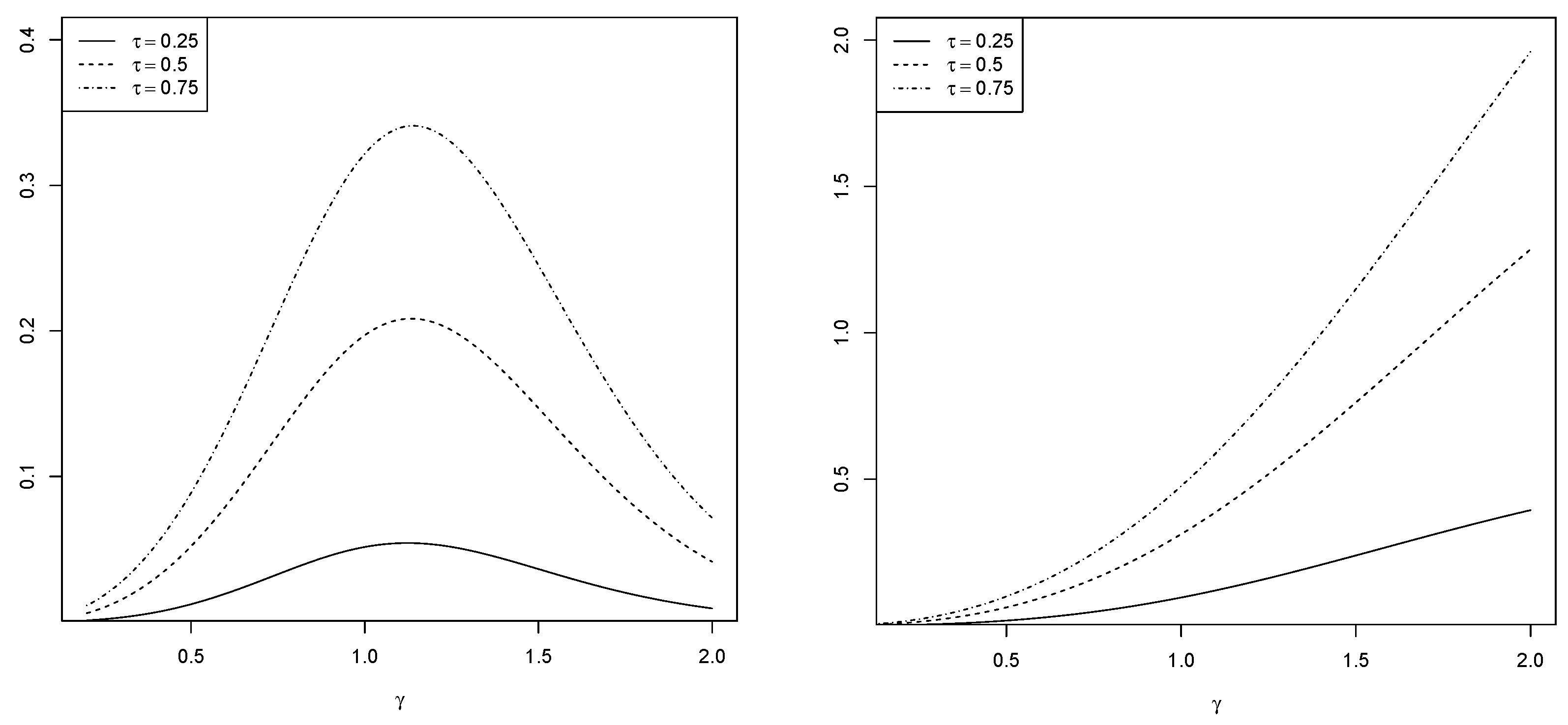
Example 1.

Assume that ${\epsilon }_i$ follows the standard log-normal distribution and is independent of $X_i$, i.e., ${ϵ}_i\sim N(0,1)$, then ${\gamma }^{*}\left(\tau \right)=1.12,1.13,1.14$ for $\tau =0.25,0.5,0.75$, respectively.

First, note that

$$\begin{array}{cc}\hfill B(\gamma ;\tau )=& E{\left[({\epsilon }^{\gamma }+{\epsilon }^{-\gamma })/\gamma \{\tau -I(\epsilon <1)\}\right]}^2\hfill \\ \hfill =& {(\tau -1)}^{2}E\{{({\epsilon }^{\gamma }+{\epsilon }^{-\gamma })}^2/{\gamma }^{2}I(\epsilon <1)\}+{\tau }^{2}E\{{({\epsilon }^{\gamma }+{\epsilon }^{-\gamma })}^2/{\gamma }^{2}I(\epsilon \ge 1)\}.\hfill \end{array}$$

By the definition,

$$\begin{array}{cc}\hfill & E\left({\epsilon }^{2\gamma }I(\epsilon <1)\right)=\frac{exp\left(2{\gamma }^2\right)}{\sqrt{2\pi }}{\int }_{-\infty }^{0}exp\left\{-{(x-2\gamma )}^2/2\right\}dx=exp\left(2{\gamma }^2\right)\Phi (-2\gamma ),\hfill \\ \hfill & E\left({\epsilon }^{-2\gamma }I(\epsilon <1)\right)=\frac{exp\left(2{\gamma }^2\right)}{\sqrt{2\pi }}{\int }_{-\infty }^{0}exp\left\{-{(x+2\gamma )}^2/2\right\}dx=exp\left(2{\gamma }^2\right)\Phi \left(2\gamma \right),\hfill \end{array}$$

hence, $B(\gamma ;\tau )=\{{\tau }^2+{(1-\tau )}^2\}\{exp\left(2{\gamma }^2\right)+2\}/{\gamma }^2$. We can derive

$$\begin{array}{cc}\hfill & E\left\{{\epsilon }^{\gamma }(\tau -I(\epsilon <1))\right\}\hfill \\ \hfill =& \frac{1}{\sqrt{2\pi }}{\int }_{-\infty }^{+\infty }exp\left(\gamma x\right)(\tau -I(x<0))exp(-x^2/2)dx\hfill \\ \hfill =& \frac{1}{\sqrt{2\pi }}\left\{(\tau -1){\int }_{-\infty }^{0}exp\left(\gamma x\right)exp(-x^2/2)dx+\tau {\int }_0^{+\infty }exp\left(\gamma x\right)exp(-x^2/2)dx\right\}\hfill \\ \hfill =& exp({\gamma }^2/2)\{(\tau -1)\Phi (-\gamma )+\tau (1-\Phi (-\gamma ))\}\hfill \\ \hfill =& exp({\gamma }^2/2)\{\tau -\Phi (-\gamma )\}.\hfill \end{array}$$

Thus, we have

$$\begin{array}{cc}\hfill {\left\{J_{\gamma }\left(\tau \right)+f_{\epsilon }\left(1\right)\right\}}^{-2}B(\gamma ;\tau )=& \frac{\{{\tau }^2+{(1-\tau )}^2\}\{exp\left(2{\gamma }^2\right)+2\}}{{\gamma }^2{\left[exp({\gamma }^2/2)\{\tau -\Phi (-\gamma )\}+f_{\epsilon }\left(1\right)\right]}^2}.\hfill \end{array}$$

There is no closed form solution for minimizing ${\left\{J_{\gamma }\left(\tau \right)+f_{\epsilon }\left(1\right)\right\}}^{-2}B(\gamma ;\tau )$, but through a numerical procedure, we find that ${\left\{J_{\gamma }\left(\tau \right)+f_{\epsilon }\left(1\right)\right\}}^2/B(\gamma ;\tau )$ reaches the maximum at $1.12$, $1.13$, and $1.14$, see Figure 2, for $\tau =0.25,0.5,0.75$, respectively. □

Example 2.

If ${ϵ}_i\sim \mathrm{Unif}(-1,1)$, then ${\gamma }^{*}\left(\tau \right)\equiv \mathsf{\Gamma }$ for any $\tau \in (0,1)$. In particular, ${\gamma }^{*}\left(\tau \right)\equiv 2$ if we set $\mathsf{\Gamma }=2$.

First, by $E\left\{{({\epsilon }^{\gamma }+{\epsilon }^{-\gamma })}^{2}I(\epsilon <1)\right\}=E\left\{{({\epsilon }^{\gamma }+{\epsilon }^{-\gamma })}^{2}I(\epsilon \ge 1)\right\}=2+\{exp\left(2\gamma \right)-exp(-2\gamma )\}/\left(4\gamma \right),$ we know that $B(\gamma ;\tau )=\{{\tau }^2+{(1-\tau )}^2\}\left[\{exp(2\gamma )-exp(-2\gamma \left)\right\}/\left(4\gamma \right)+2\right]/{\gamma }^2$. It further leads to

$$\begin{array}{cc}\hfill E\left\{{\epsilon }^{\gamma }(\tau -I(\epsilon <1))\right\}=& \frac{1}{2}{\int }_{-1}^{1}exp\left(\gamma x\right)\{\tau -I(x<0)\}dx\hfill \\ \hfill =& \frac{1}{2\gamma }\left\{(\tau -1){\int }_{-1}^{0}exp\left(\gamma x\right)d\left(\gamma x\right)+\tau {\int }_0^{1}exp\left(\gamma x\right)d\left(\gamma x\right)\right\}\hfill \\ \hfill =& \{\tau exp(\gamma )+(1-\tau )exp(-\gamma )-1\}/\left(2\gamma \right),\hfill \end{array}$$

and then we have

$$\begin{array}{cc}\hfill & {\left\{J_{\gamma }\left(\tau \right)+f_{\epsilon }\left(1\right)\right\}}^{-2}B(\gamma ;\tau )\hfill \\ \hfill =& \frac{\{{\tau }^2+{(1-\tau )}^2\}\{8\gamma +exp\left(2\gamma \right)-exp(-2\gamma )\}}{\gamma {\left[\{\tau exp\left(\gamma \right)+(1-\tau )exp(-\gamma )-1\}+2\gamma f_{\epsilon }\left(1\right)\right]}^2}\hfill \end{array}$$

As is shown in Figure 2, ${\left\{J_{\gamma }\left(\tau \right)+f_{\epsilon }\left(1\right)\right\}}^2/B(\gamma ;\tau )$ reaches the maximum at $\mathsf{\Gamma }$. □

4. Simulation Study

For numerical implementation of the proposed method, we first obtained ${\widehat{\beta }}_n(\gamma ;\tau )$ by minimizing (4) for each fixed $\gamma \in [0,\mathsf{\Gamma }]$ using the Nelder–Mead simplex algorithm, and then tuned and selected $\gamma \left(\tau \right)$ based on a criterion. We finally obtained the adapted value $\widehat{\gamma }\left(\tau \right)$ and the corresponding coefficient ${\widehat{\beta }}_n(\widehat{\gamma };\tau )$. To verify the theoretical properties of the proposed method, we conducted simulation studies under two simple scenarios with finite samples to illustrate the proposed method.

Scenario 1. We considered a simple univariate, case,

$$Y_i=\alpha +\beta X_i+{ϵ}_i,i=1,\dots ,n,$$

where $\alpha =0$, $\beta =1$, $X_i$ follows the standard normal distribution, and ${ϵ}_i={ϵ}_i^{*}-{\Phi }^{-1}\left(\tau \right)$, with ${ϵ}_i^{*}$ following the standard normal distribution and ${\Phi }^{-1}\left(\tau \right)$ indicating the $\tau$-quantile of the standard normal distribution. We set the sample size $n=200,400$ and the number of replications as 500.

For Scenario 1, ${\beta }_0$ is of one dimension. So, we can plot the 3-dimensional surface of $W_n(\beta ,\gamma ;\tau =0.5)$, see Figure 3, which shows that $W_n(\beta ,\gamma ;\tau )$ is local convex with respect to both $\gamma$ and $\beta$. As illustrated previously in Example 1, if $ϵ$ follows the standard normal distribution, the true value of ${\gamma }^{*}\left(\tau \right)$ in theory is around $1.08$ by criterion (II).

Table 1. Simulation results under Scenario 1.

			${\mathit{\beta }}_0=1$				$\mathit{\gamma }$
Criterion	$\mathit{n}$	$\mathbf{\tau }$	Est.	SD	SE	CP%	Est.	SD
I	200	$0.25$	$0.995$	$0.067$	$0.069$	$94.8$	$0.000$	$0.000$
		$0.50$	$1.003$	$0.060$	$0.063$	$95.2$	$0.000$	$0.000$
		$0.75$	$1.001$	$0.073$	$0.070$	$93.0$	$0.000$	$0.000$
	400	$0.25$	$0.998$	$0.047$	$0.049$	$94.4$	$0.000$	$0.000$
		$0.50$	$0.999$	$0.044$	$0.044$	$93.0$	$0.000$	$0.000$
		$0.75$	$1.000$	$0.048$	$0.049$	$93.4$	$0.000$	$0.000$
II	200	$0.25$	$0.999$	$0.056$	$0.052$	$93.8$	$1.048$	$0.321$
		$0.50$	$1.002$	$0.057$	$0.050$	$93.6$	$1.070$	$0.339$
		$0.75$	$1.000$	$0.060$	$0.051$	$92.6$	$1.068$	$0.339$
	400	$0.25$	$1.002$	$0.041$	$0.039$	$94.0$	$1.126$	$0.246$
		$0.50$	$1.000$	$0.041$	$0.038$	$94.8$	$1.136$	$0.261$
		$0.75$	$0.999$	$0.042$	$0.039$	$93.5$	$1.137$	$0.242$
III	200	$0.25$	$0.996$	$0.051$	$0.054$	$96.2$	$0.781$	$0.234$
		$0.50$	$0.998$	$0.056$	$0.051$	$91.4$	$0.722$	$0.266$
		$0.75$	$0.999$	$0.061$	$0.054$	$90.8$	$0.760$	$0.248$
	400	$0.25$	$0.996$	$0.039$	$0.040$	$94.0$	$0.773$	$0.205$
		$0.50$	$1.001$	$0.038$	$0.037$	$94.8$	$0.713$	$0.216$
		$0.75$	$1.002$	$0.042$	$0.038$	$92.4$	$0.761$	$0.206$

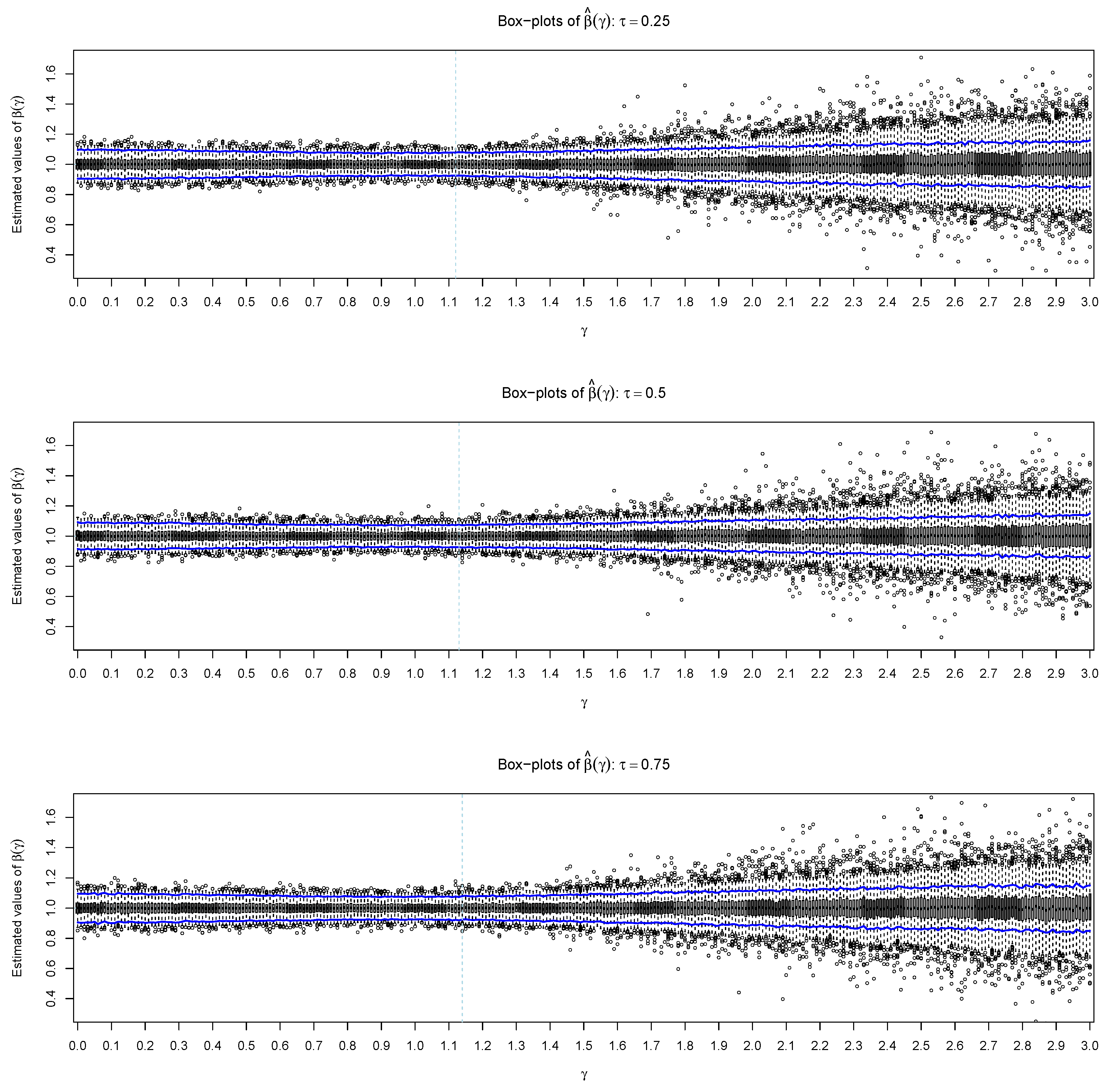
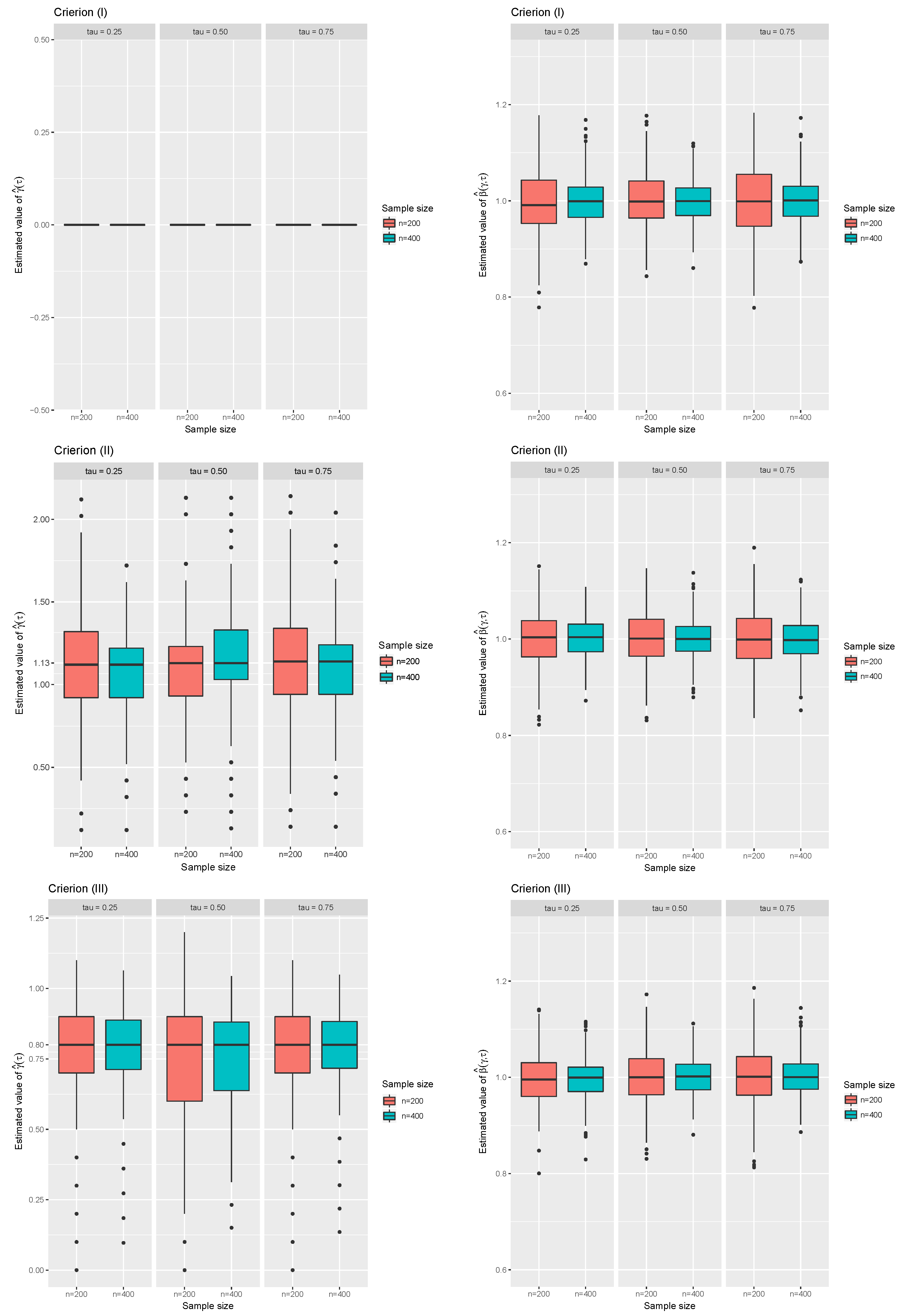
NOTE: Est., the empirical mean of the estimated coefficients; SD, the sample standard deviation of the estimated coefficients; SE, the empirical mean of standard errors based on the bootstrap method; CP, the coverage probability of the 95% confidence intervals.

summarizes the simulation results at different quantiles with various adaptive criteria. The results show that the estimated regression coefficients have small biases, and the biases demonstrate a clear trend of asymptotic consistency for all settings. According to the results in Table 1 and the box-plots in Figure 4 and Figure 5, we also see that the adaptive parameter $\widehat{\gamma }\left(0.5\right)$ selected by criteria (I) and (II) converge to 0.0, 1.13 and 0.8, respectively. 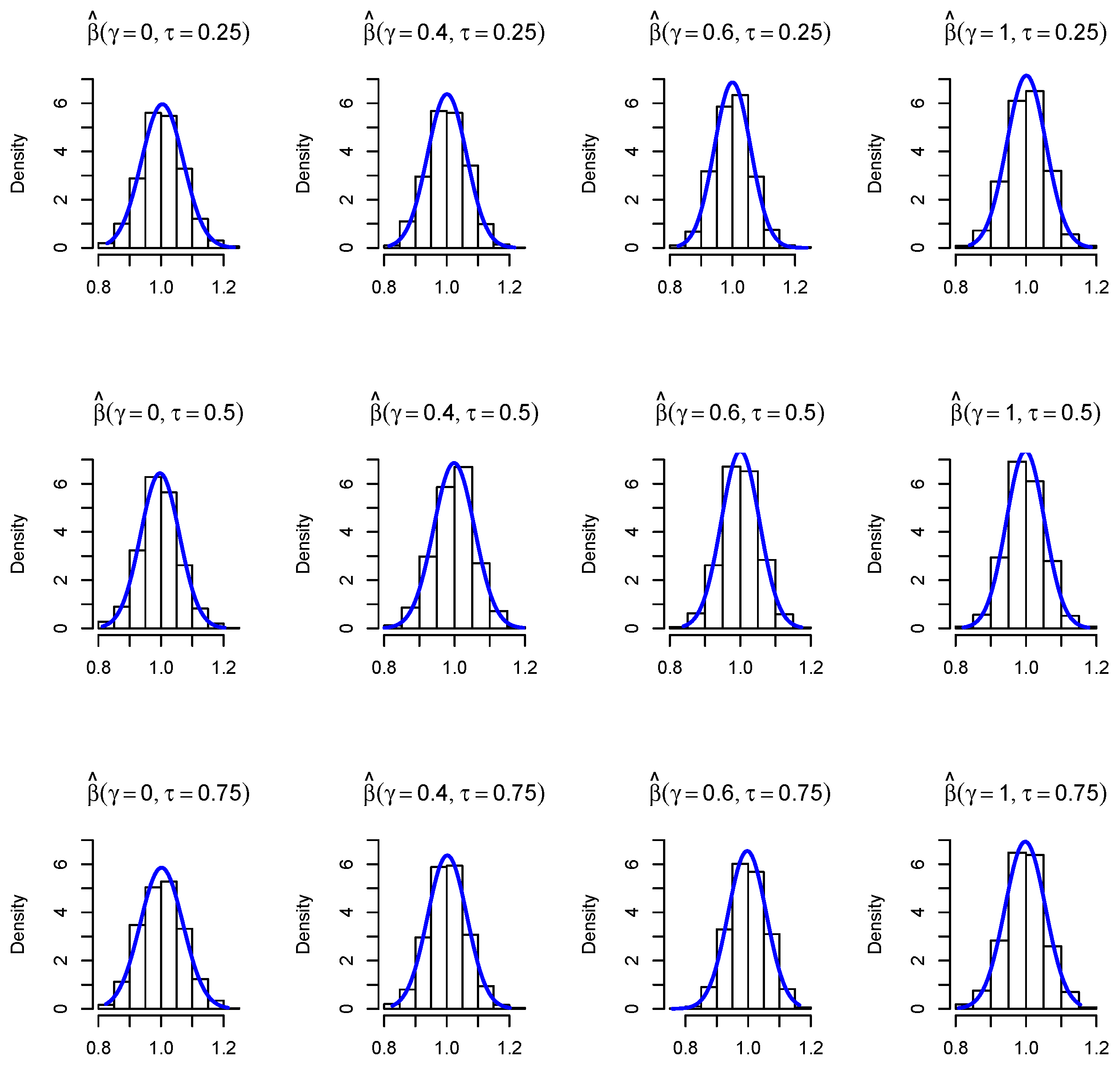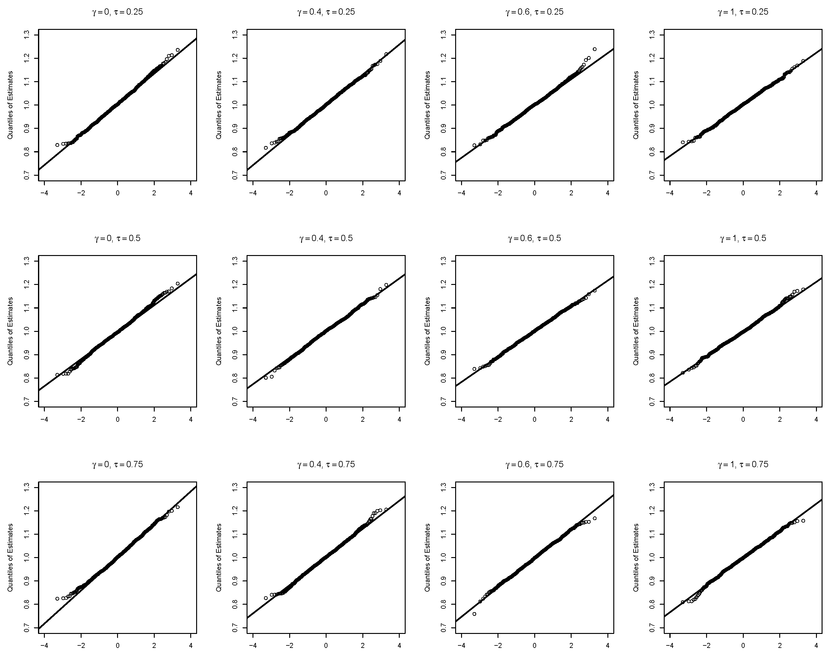The values of $\gamma \left(\tau \right)$ by criterion (I) are all equal to 0, indicating the estimates by criterion (I) are equivalent to that by the traditional quantile regression. Compared to the estimate by traditional quantile regression, the proposed estimate under the adaptive criterion (II) enhances the estimation efficiency of coefficients by 5∼20%. Additionally, from the histogram in Figure 6 and the quantile–quantile (Q–Q) plot [21,22] in Figure 7, we see that the empirical distribution of the estimators follows a clear normal distribution.

Scenario 2. We considered the same model and settings as in Scenario 1, except that the error follows a uniform distribution, and ${ϵ}_i={ϵ}_i^{*}-Q_{{ϵ}^{*}}\left(\tau \right)$, where ${ϵ}_i^{*}$ follows $\mathrm{Uniform}(-1,1)$, and $Q_{{ϵ}^{*}}\left(\tau \right)=2\tau -1$.

The simulation results are presented in

Table 2. Simulation results under Scenario 2.

			${\mathit{\beta }}_0=1$				$\mathit{\gamma }$
Criteria	$\mathit{n}$	$\mathbf{\tau }$	Est.	SD	SE	CP%	Est.	SD
I	200	$0.25$	$1.005$	$0.062$	$0.063$	$95.0$	$0.000$	$0.000$
		$0.50$	$1.005$	$0.072$	$0.073$	$95.0$	$0.000$	$0.000$
		$0.75$	$0.997$	$0.066$	$0.063$	$93.4$	$0.000$	$0.000$
	400	$0.25$	$1.000$	$0.043$	$0.043$	$94.8$	$0.000$	$0.000$
		$0.50$	$0.999$	$0.052$	$0.052$	$94.4$	$0.000$	$0.000$
		$0.75$	$0.999$	$0.043$	$0.045$	$95.2$	$0.000$	$0.000$
II	200	$0.25$	$0.998$	$0.038$	$0.039$	$94.0$	$1.927$	$0.250$
		$0.50$	$0.999$	$0.037$	$0.038$	$95.2$	$1.996$	$0.081$
		$0.75$	$1.001$	$0.038$	$0.040$	$92.8$	$1.924$	$0.257$
	400	$0.25$	$1.001$	$0.027$	$0.026$	$95.8$	$1.940$	$0.221$
		$0.50$	$0.999$	$0.026$	$0.026$	$95.0$	$1.998$	$0.036$
		$0.75$	$1.000$	$0.027$	$0.029$	$94.0$	$1.942$	$0.201$

NOTE: Est., the empirical mean of the estimated coefficients; SD, the sample standard deviation of the estimated coefficients; SE, the empirical mean of the estimated standard errors based on the bootstrap method; CP, the coverage probability of the 95% confidence intervals.

. It is shown that under criterion (I) that the estimated values of ${\gamma }^{*}\left(\tau \right)$ are all equal to 0 as well, and the corresponding estimated coefficients at different quantiles have small biases and reasonable coverage probabilities. Under the adaptive criterion (II), the estimated values of ${\gamma }^{*}\left(\tau \right)$ tend to converge to $\mathsf{\Gamma }=2$. In addition, the regression coefficients are all estimated accurately. Overall, the simulation results in Table 2 match well with the theoretical properties in Example 2 in Section 4. Specifically, the estimation efficiency of coefficients using the proposed method with criterion (II) increases by 60∼100% over the traditional quantile regression.

5. Application

We applied the proposed method to a prostate cancer study [23], where the prostate cancer data contain the medical records of 97 male patients who received a radical prostatectomy. The description of data is summarized in

Table 3. Summary of prostate cancer data.

Components	Total	Components	Total
cancer volume (cc)		PSA (ng./mL.)
mean (SD)	7.0 (7.9)	mean (SD)	23.74 (40.8)
median	4.25	median	13.35
range	45.39	range	265.2
prostate weight (gm.)		capsular penetration (cm.)
mean (SD)	45.5 (45.6)	mean (SD)	2.36 (3.72)
median	37.45	median	0.45
range	438.5	range	18.0
Age (year)		Gleason score –no.(%)
mean (SD)	63.9 (7.45)	= 6	35 (36)
median	65.00	= 7	56 (58)
range	38.00	= 8	1 (1)
		= 9	5 (5)
BPHA (cm${}^2$)		Percentage of Gleason
mean (SD)	2.64 (2.94)	scores 4 or 5 –no.(%)
median	1.35	$[0,20]$	61 (63)
range	9.99	$(20,60]$	24 (25)
SVI -no. (%)		$(60,100]$	12 (12)
+	21 (22)
−	76 (78)

NOTE: ‘SVI’, seminal vesicle invasion; ‘BPHA’, benign prostatic hyperplasia amount.

.

The response variable of interest is the level of prostate antigen (PSA), and there are eight predictor variables, including the log of cancer volume, the log of prostate weight, age, the log of the amount of benign prostatic hyperplasia, seminal vesicle invasion, the log of capsular penetration, Gleason score and the percentage of Gleason scores of 4 or 5. The research goal is to study the covariate effects of the predictor variables at the level of prostate antigen.

We considered a linear quantile model for the association between prostate antigen and the predictor variables. For convenience, we first standardized the predictors as well as the dependent variables, and then included the intercept in the model. We took 200 bootstrap samples for the variance estimation of coefficients, and selected the adaptive parameter using criterion (II). We obtained the estimate $\widehat{\gamma }\left(\tau \right)=2.0$ for all grid points $\tau \in \{0.1,0.2,\dots ,0.8,0.9\}$. Then, we further acquired the estimated regression coefficients with 95% Confidence Intervals (CIs) at the 0.25, 0.50 and 0.75 quantiles, which are summarized in

Table 4. The estimated covariate effects with 95% CIs for the prostate cancer study.

	Traditional QR (Criterion (I))		Criterion (II)
Coeff. $\widehat{\mathbf{\beta }}\left(\mathbf{\tau }\right)$	Est.	95% CI	Est.	95% CI	CI Ratio
$\tau =0.25$
Intercept	$-0.354$	$(-0.513,-0.167)$	$-0.217$	$(-0.333,-0.102)$	$1.498$
Volume	$0.696$	$(0.486,0.864)$	$0.611$	$(0.450,0.772)$	$1.174$
Weight	$0.282$	$(0.135,0.473)$	$0.238$	$(0.101,0.374)$	$1.238$
Age	$-0.033$	$(-0.203,0.150)$	$-0.147$	$(-0.272,-0.023)$	$1.418$
Hyperplasia	$0.130$	$(0.007,0.435)$	$0.102$	$(-0.039,0.244)$	$1.512$
Seminal	$0.275$	$(0.087,0.408)$	$0.248$	$(0.113,0.383)$	$1.189$
Capsular	$-0.259$	$(-0.504,-0.090)$	$-0.150$	$(-0.324,0.024)$	$1.190$
Gleason	$-0.022$	$(-0.189,0.152)$	$0.039$	$(-0.137,0.215)$	$0.969$
Percentage	$0.246$	$(-0.091,0.480)$	$0.128$	$(-0.048,0.305)$	$1.618$
$\tau =0.5$
Intercept	$-0.057$	$(-0.185,0.071)$	$0.009$	$(-0.090,0.109)$	$1.286$
Volume	$0.544$	$(0.363,0.725)$	$0.601$	$(0.459,0.742)$	$1.279$
Weight	$0.239$	$(0.059,0.419)$	$0.220$	$(0.091,0.349)$	$1.395$
Age	$-0.173$	$(-0.307,-0.039)$	$-0.116$	$(-0.222,-0.010)$	$1.264$
Hyperplasia	$0.201$	$(0.042,0.360)$	$0.112$	$(-0.004,0.228)$	$1.371$
Seminal	$0.287$	$(0.087,0.487)$	$0.240$	$(0.095,0.386)$	$1.375$
Capsular	$-0.159$	$(-0.343,0.026)$	$-0.111$	$(-0.274,0.052)$	$1.132$
Gleason	$0.127$	$(-0.050,0.304)$	$0.071$	$(-0.087,0.230)$	$1.117$
Percentage	$0.099$	$(-0.050,0.248)$	$0.084$	$(-0.081,0.248)$	$0.906$
$\tau =0.75$
Intercept	$0.378$	$(0.312,0.514)$	$0.253$	$(0.143,0.363)$	$0.918$
Volume	$0.570$	$(0.348,0.752)$	$0.592$	$(0.452,0.733)$	$1.438$
Weight	$0.136$	$(-0.067,0.342)$	$0.199$	$(0.058,0.339)$	$1.456$
Age	$-0.135$	$(-0.305,0.035)$	$-0.121$	$(-0.241,-0.002)$	$1.423$
Hyperplasia	$0.155$	$(-0.021,0.333)$	$0.087$	$(-0.048,0.222)$	$1.311$
Seminal	$0.334$	$(0.198,0.439)$	$0.261$	$(0.186,0.405)$	$1.100$
Capsular	$-0.089$	$(-0.383,0.065)$	$-0.070$	$(-0.227,0.088)$	$1.422$
Gleason	$-0.061$	$(-0.210,0.143)$	$-0.019$	$(-0.161,0.123)$	$1.243$
Percentage	$0.170$	$(-0.016,0.226)$	$0.125$	$(-0.059,0.308)$	$0.659$

, where the results are also compared to those of the traditional quantile regression. As is shown in the table, there is not much difference between the estimated coefficients by the traditional quantile regression and the proposed method with criterion (II). However, referring to the values of the ‘CI ratio’ (‘CI Ratio’ is defined as the ratio of the length of 95% CI by traditional QR over that by the proposed method using criterion (II)), we can see overall that the lengths of 95% CIs by the proposed method are significantly smaller than that by a traditional quantile regression. 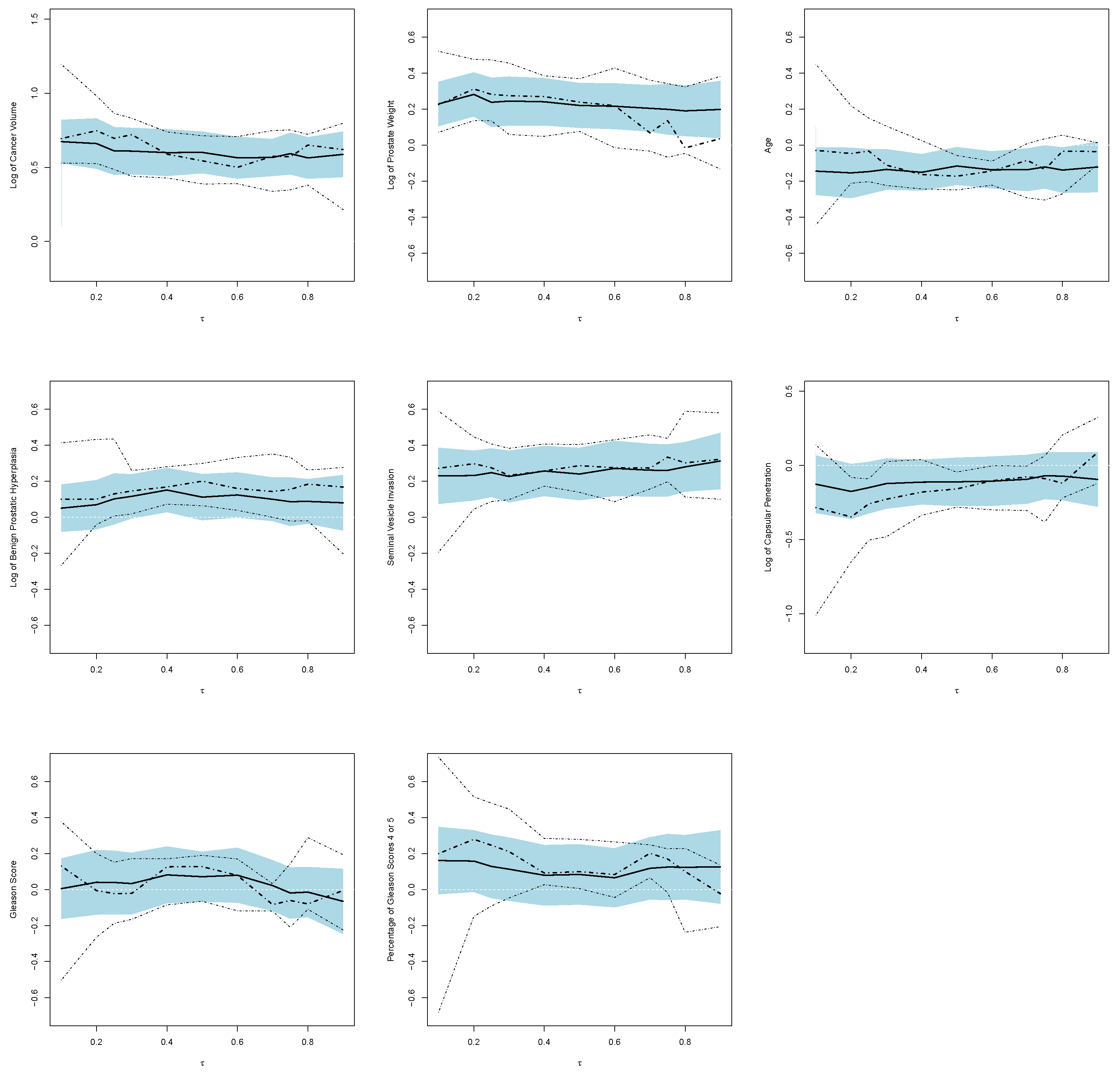Figure 8 presents the estimated curves of coefficients with 95% confidence bands. The figure shows that the proposed method with criterion (II) provides smoother estimates and more stable and narrower confidence bands compared to those by a regular quantile regression, especially at the region of tail quantiles. From the results in both Table 4 and Figure 8, we concluded that the cancer volume, the prostate weight, and the seminal vesicle invasion are significantly associated with the level of prostate antigen, which is as expected since a high level of prostate antigen is generally regarded as strong evidence of prostate cancer. While the effects of the amount of benign prostatic hyperplasia, capsular penetration, Gleason score and the percentage of Gleason scores of 4 or 5 at the level of prostate antigen are statistically insignificant.

6. Discussion

We propose a general class of loss functions to conduct a quantile regression, which naturally unifies the absolute and the relative error criteria. The consistency and asymptotic normality of the resulting estimators are established. Numerical studies demonstrate the good performance of the proposed method using finite samples. Although our proposal is based on a quantile regression, similar ideas can also be extended to other statistical framework such as the M-estimator. Further research includes extending the proposed procedure to censored data, see, e.g., [7,24,25], or longitudinal data [6,26], and even to the case with a diverging number of parameters or ultra-high dimensionality situations [27].