Efficient Processing of All Nearest Neighbor Queries in Dynamic Road Networks

Abstract

The increasing trend of GPS-enabled smartphones has led to the tremendous usage of Location-Based Service applications. In the past few years, a significant amount of studies have been conducted to process All nearest neighbor (ANN) queries. An ANN query on a road network extracts and returns all the closest data objects for all query objects. Most of the existing studies on ANN queries are performed either in Euclidean space or static road networks. Moreover, combining the nearest neighbor query and join operation is an expensive procedure because it requires computing the distance between each pair of query objects and data objects. This study considers the problem of processing the ANN queries on a dynamic road network where the weight, i.e., the traveling distance and time varies due to various traffic conditions. To address this problem, a shared execution-based approach called standard clustered loop (SCL) is proposed that allows efficient processing of ANN queries on a dynamic road network. The key concept behind the shared execution technique is to exploit the coherence property of road networks by clustering objects that share common paths and processing the cluster as a single path. In an empirical study, the SCL method achieves significantly better performance than competitive methods and efficiently reduces the computational cost to process ANN queries in various problem settings.

1. Introduction

Over the years, mobile technologies and location-based services (LBSs) have rapidly become popular, affording its user’s easy access to a variety of LBSs that aim to provide value-added experiences. On the other hand, GPS-enabled devices, such as smartphones, wireless sensor networks (WSN), and navigation systems, are responsible for generating a massive number of spatial query requests. The most common instances of spatial queries [1] associated with popular LBSs include shortest path queries, range queries [2,3], k-nearest neighbor (k-NN) queries [4,5], reverse k-NN queries [6], and preference queries [7,8,9]. To address the growing demand for such services, a significant amount of research has been conducted over the past few years to monitor and improve the processing of spatial queries. All these spatial queries extract the data objects based on the distance from the query point.

The ANN query retrieves all nearest neighbor data objects for every query object with the least distance between them. It can be said that ANN is a variation of k-NN, where the k is always equal to one for each query object in the entire query dataset. In this paper, the exploration of the ANN queries on a dynamic road network is carried out as it serves as a close approximation to real-world scenarios. Due to the frequent traffic updates, the weights, i.e., traveling time and distance, change accordingly. ANN queries can be used in real-life applications such as “Find the nearest gas station for every car-parking lot”, and in case of ride-sharing, “Find all the nearest taxi for all the matched customers”. In a ride-sharing scenario, a car is shared by one or more passengers. Let us assume that the group of passengers is requesting the nearest vacant taxi cab via their smartphones. The groups of passengers and taxi cabs are denoted as query objects and data objects, respectively. The scheduling system assigns the taxi cab that bears the smallest traveling distance to all the passengers. The consequence demand for real-time reporting in the ride-sharing concept can be facilitated through the improvement in ANN queries. The aforementioned examples utilize the snapshot query because the huge number of LBSs involve only snapshot query processing capabilities [10,11,12,13,14,15], rather than continuous monitoring.

A naive approach to process ANN queries is to scan the whole dataset by computing the distance between each query and data object. For large datasets, such a naive solution is not feasible because of its high computational complexity. Until now, most of the research on ANN queries has been done in Euclidean and metric space [16,17,18]. Their approaches either focus on the indexing scheme to implement the pruning that mitigates the entire scanning of the dataset or precomputation of the shortest path distance. These approaches are not suitable in the context of dynamic road networks as materialized structures cannot dynamically compute the shortest path between each pair of nodes in road networks, and they are limited to computation of Euclidean distances. For example, let us consider a scenario with a huge number of query objects requesting for their respective nearest data object within the same time frame $t_1$. Indexing such a large number of query objects with regard to their locations and distances to evaluate the set of nearest neighbors (NNs) might be suitable for a one-time evaluation. Whenever there occurs any location update after a certain time duration $t_{i+1}$, the server would be required to rebuild the whole index from the start, which would result in a huge computational burden. However, using the snapshot of the query locations at each time frame $t_{i+1}$ and clustering them would reduce the redundant network traversal regardless of the movement of the query object. Nevertheless, if the query object moves away from its current query cluster, then re-clustering would take relatively less time compared to the indexing, which makes it feasible for dynamic road environments.

Unfortunately, the indexing method cannot support answering ANN queries in dynamic road networks due to the computation overhead. Therefore, this study proposes an efficient algorithm to find the ANN queries on dynamic road networks by implementing the shared execution technique. The fundamental idea of the shared-execution technique is to batch the queries and execute them as a single query in order to achieve efficient load handling [19,20]. Standard clustered loop (SCL), based on the shared-execution technique, follows a similar rule, according to which groups of similar objects are clustered together. The working sets of SCL are constructed in two steps. In the first step, objects belonging to similar categories are clustered and arranged into a sequence. During the second step, a maximum of two NN queries are evaluated at the ends of each query object cluster and the results are assigned to all query objects belonging to that cluster. SCL exhibits low computational demands as it avoids the evaluation of redundant NN queries by employing shared-execution processing. SCL does not implement any materialization or precomputing scheme to process NN queries. Any existing nearest neighbor algorithm can be incorporated to process the ANN. The primary contributions of this study can be outlined as follows:

• The shared-execution based SCL method is proposed for the efficient processing of ANN queries on dynamic road networks. Moreover, to the extent of our knowledge, this is the first attempt to evaluate ANN queries on dynamic road networks.
• The proposed SCL method is simple and easy to implement. Only an optimized number of NN queries are evaluated by implementing clustering and shared-execution.
• Extensive experiments with various settings are performed to measure the superiority of the proposed scheme for particular scenarios.

The rest of the paper is organized as follows. Related works have been discussed in Section 2. An overview of the associated concepts is presented in Section 3. The SCL algorithm is outlined in Section 4 and Section 5. The time complexity of the proposed algorithm is discussed in Section 5.3. The experiments and evaluation of the proposed method are exhibited in Section 6 and further discussion in Section 7. Finally, the paper is concluded with future research direction in Section 8.

2. Related Works

2.1. Dynamic Road Network

Currently, the processing of spatial queries on road networks has intrigued many researchers. The known developments can be chronicled as follows. Papadias et al. [21] introduced Incremental Euclidean Restriction (IER) and Incremental Network Expansion (INE), both of which apply multi-step kNN capable of retrieving high-dimension similarities. IER is an early kNN technique that inherits its characteristics from the A* search algorithm [17]. It operates on the assumption that the network distance between two distinct objects cannot be less than the Euclidean distance between them. INE, on the other hand, performs spatial search by expanding the search region from a query object. The first data object discovered during the expansion is identified to be the data object closest to the initial query object. Samet et al. [22] proposed the SILC framework to mitigate the storage cost incurred during the decoupling of the objects from a large spatial network. SILC precomputes the shortest path between all possible pairs of nodes based on a best-first-search manner and uses quad-trees to store the identified shortest paths. Lee et al. [23] suggest route overlay and association directory (ROAD), a framework to search the spatial objects lying on the road network that cleanly separates the road network and objects. It is a solution-based approach that utilizes some precomputed results and distance ranges, instead of using precise distances that consume redundant storage. Hence, ROAD aims to solve the problem of high precomputation and storage overhead by utilizing the search space pruning to improve the efficiency of the framework. Precomputation is an expensive operation as the result sets must be stored. To overcome this issue, Zhong et al. [24] proposed an efficient indexing scheme that recursively partitions the road network into equal sub-networks. The assembly-based method computes the shortest path distance for the single-pair shortest path (SPSF) query. A few studies exist to process an NN query on a dynamic road environment [25,26]. In these studies, the authors employed precomputed grid structures that utilized in-memory data structures. However, this is inappropriate for large networks. A safe-region technique was proposed to efficiently compute the nearest neighbor queries for moving query objects [9,27]. Techniques involving safe-region computation cannot be used to process ANN queries on dynamic road networks considering the difference in problem definition. Heuristic methods were developed to compute the shortest path in dynamic road networks [28,29,30]. These methods depend on a lightweight indexing technique for route planning in dynamic road networks. However, these methods cannot be applied directly to process ANN queries on dynamic road networks considering the differences in the motivation of studies.

2.2. All Nearest Neighbor Queries

Clarkson [16] proposed three different algorithms to solve the problem of ANN computation in Euclidean space. Both the query and data objects were assumed to be of the same type, i.e., monochromatic data. All the data points were enclosed in small cubic cells of identical size. Then, the distance bounded by the nearest data cell represented the nearest neighbor of the query object. Zhang et al. [17] proposed a two-phase hash-based algorithm that loads pairs of data and query objects and divides them into buckets of equal size. Identical or overlapping buckets can then be used to identify the nearest neighbor of each query object. To date, there is only one study of the problem of processing ANN query in road networks [18]. This study introduced virtual vertex traversal (VIVET), which uses an index-based algorithm and performs a single traversal from a virtual node to all other existing nodes, and their shortest-path distances are stored in an array used for precomputation. Subsequently, a simple lookup in the array allows finding the nearest neighbor of any query object. However, the creation of an index is memory-intensive. No precomputation or indexing scheme can solve the problem of finding the ANN on dynamic road networks without incurring high computational costs. The proposed scheme differs from the existing studies in various aspects. First, the proposed method takes into account the dynamic nature of the road network, which cannot be addressed by using precomputation. Secondly, the implementation of shared execution enables efficient query processing. Lastly, based on gained knowledge, this is the first attempt to evaluate ANN queries on dynamic road networks.

3. Preliminaries

Here, a formal definition of the basic concepts along with their characteristics that have been used in this paper is mentioned. Firstly, this section establishes fundamentals for the dynamic road networks Secondly, this provides insight about the classification of nodes, which is the basis for understanding shared execution. Lastly, the conventional definition of an ANN query is given.

3.1. Dynamic Road Network

The world is composed of various complex structures, such as biological networks, communication networks, power-grid networks, and road networks [31,32], that can be represented and analyzed using a graph where the nodes and edges resemble the entity and the relationship among them [33]. In this study, the road network is depicted as an undirected graph $G=〈N,E,W〉$, where $N,E,W$ denotes the sets of nodes, edges, and the weights. In general, each edge has a non-negative weight that represents its distance. The concept of a dynamic road network simply can be understood as the variation of the moving objects and distances depending upon the traffic and road condition at any time.

Figure 1 depicts an example of a dynamic road network, in which objects $q_1$ to $q_5$ represent query objects (denoted by rectangles), and objects $d_1$ to $d_4$ represent data objects (denoted by triangles). Let us interpret this example in terms of a ride-sharing service, where data objects represent taxi-cabs and query objects represent passengers. The ride-sharing service involves sending a taxi-cab to each passenger who is located within the nearest vicinity from the taxi-cab. Further, the travel time should be updated frequently by consulting the real-time traffic conditions. For example, the nearest taxi-cab for $q_5$ at time $t_1$ is $d_4$, as shown in Figure 1a. However, due to huge traffic-congestion in taxi-cab $d_4$’s locality, it is incapable of reaching $q_5$ faster than $d_3$. In this study, a dynamic graph is treated as series of snapshots, where each snapshot is static in itself, yet dynamic between each other.

3.2. Classification of Nodes

In this study, nodes are classified into three different categories. Here, the degree of a node refers to the number of adjacent nodes that it is connected with. If the degree of a node is equal to one or two, then the node is called terminal or intermediate node, respectively. If the degree of a node is more than two, it is called an intersection node.

Node Sequence and Segments

A node sequence $\overline{n_l{n}_{l+1}\dots n_m}$ represents a path between two nodes $n_l$ and $n_m$ in a road network, such that $n_l$ and $n_m$ are either intersection nodes or a terminal nodes, and $n_{l+1},\dots ,n_{m-1}$ are intermediate nodes. The node sequence from $n_l$ to $n_m$ can be called a node segment. The shortest path distance is a distance between a data object and query object, whereas the length denotes the distance of the path from that query object to the data object in the same node sequence.

Table 1. Notation and their meaning.

Notation	Meaning
q	Query object $q\in Q$.
d	Data object $d\in D$.
$\overline{n_l{n}_{l+1}\dots n_m}$	Node sequence $\overline{N}$ when $n_l$ and $n_m$ are either intersection nodes or terminal nodes, $\overline{n_l{n}_m}\in \overline{\left|N\right|}$
$\overline{q_i{q}_{i+1}\dots q_j}$	Query sequence $\overline{Q}$ generated from query objects $q_i,q_{i+1},\dots q_j$ in the same node sequence, $\overline{q_i{q}_j}\in \overline{\left|Q\right|}$
D($\overline{q_i{q}_j})$	Set of data objects located in query object cluster $\left(\overline{q_i{q}_j}\right)$.
$D^q$	Set of data objects closest to query objects q for every d.
$dist(q,d)$	Shortest path distance between the data object and the query object.
$len(q,d)$	Distance of the segment connecting q and d such that they lie in the same segment.

summarizes the notations used in this paper. For simplification of notation, $\overline{q_i{q}_j}$ is used to indicate the query object cluster, i.e., $\overline{q_i{q}_{i+1}\dots q_j}$, where, $q_i{q}_{i+1},\dots ,q_j$ are the query objects lying in the same node segment.

3.3. All Nearest Neighbor Query

The ANN query in a road network returns all the pairs of every query object with the corresponding closest data object.

Definition 1.

Given two different object sets Q and D, where $Q=\left\{q_1,q_2,\dots ,q_n\right\}$ and $D=\left\{d_1,d_2,\dots ,d_m\right\}$, the ANN query returns the set of pair of objects from $Q\bowtie D$ such that D is the nearest neighbor of Q.

$$Q\bowtie D=\left\{〈q,d〉|\forall q\in Q,\forall d\in D^q\right\}$$

4. Methods of Clustering Query Objects

4.1. Methodology

An overview of the proposed query processing methodology has been depicted in Figure 2. Initially, the server captures a snapshot and creates a query processing module, which includes the query locations and n number of generated query requests at a time $t_1$ (Step 1 in Figure 2). Following this, the query processing module begins to search the nearest data object (Step 2 in Figure 2). During the search, the SCL method first traverses through the network and clusters all nodes that are in the same node segment, i.e., ‘$intermediatenodes$’. The node clustering process takes place only once and is used for the next snapshot (Step 3 in Figure 2). In addition, the query objects located in the same node cluster will be grouped together to form a cluster of query objects after scanning each node cluster (Step 4 in Figure 2). Next, the NN query is evaluated at the boundaries of each query object cluster. For every query object cluster, the generated NN result will be used for comparing the distance between the inner query objects with boundary query objects if the query object cluster size is equal or more than three. This process eliminates the necessity to perform traversal for inner query objects. The results of the boundary query objects are assigned to the nearest inner query objects (Step 5 in Figure 2). Finally, the result set that contains the nearest data object for each query object is returned to corresponding query users (Step 6 in Figure 2). After $t_{i+1}$ time, the process is repeated to update the result set and return fresh query responses.

4.2. Clustering Algorithm

Clustering is a process that involves the grouping of the data points belonging to the same category. There are two distinct types of clustering used: node and query object clustering. Figure 3a represents node clusters (denoted by different lines) in a road network. After clustering, the following node sequences are formed: $\overline{n_1{n}_2{n}_3}$, $\overline{n_1{n}_4{n}_3}$ and $\overline{n_1{n}_3}$.

Figure 3b represents the clustering process of query objects in the same node sequence. There are six query objects $q_1$ to $q_6$ and four data objects $d_1$ to $d_4$. Given two objects set of $Q=\left\{q_1,q_2,q_3,q_4,q_5,q_6\right\}$ and $D=\left\{d_1,d_2,d_3,d_4\right\}$ where $q_1$, $q_5$ and $q_4$ query objects in node sequence $\overline{n_1{n}_2{n}_3}$ are clustered together into $\overline{q_1{q}_5{q}_4}$, the query objects $q_3$ and $q_2$ in the node sequence $\overline{n_1{n}_4{n}_3}$ are clustered into $\overline{q_2{q}_3}$ and a single query object $q_6$ in $\overline{n_1{n}_3}$ is clustered into $\overline{q_6}$. The bold lines represent the query object clusters. The set of query objects $Q=\left\{q_1,q_2,q_3,q_4,q_5,q_6\right\}$ is now converted into $\overline{Q}=\left\{\overline{q_1{q}_5{q}_4},\overline{q_2{q}_3},\overline{q_6}\right\}$, where $\overline{Q}$ indicates the set of query object clusters.

Algorithm 1 outlines the process for clustering the query objects into query object clusters. The clustering process incorporates two steps. Generation of the node sequence is followed by generation of the query object clusters. $Line6$ checks whether the node is an intersection node or a terminal node. If the node is either type, paths from the node to its adjacent nodes are explored until an intermediate node is found. A node sequence is added to the $\overline{N}$. From $Lines$ 15–18, the algorithm looks for the query objects in each node sequence. Then, the discovered objects are grouped together and a query object cluster is formed and added to $\overline{Q}$ as in $Line17$. $Line19$ returns the final set of query object clusters.

Algorithm 1: Cluster_Query_Objects $\left(Q,N,E\right)$

5. SCL Design

5.1. Overview of SCL

Cho [34] suggests that evaluating NN queries at the two ends of the query object cluster is adequate to retrieve the nearest data object for every query object. According to Lemma 1, after evaluating at most two NN queries for $q_i$ and $q_j$, located at the boundaries of the query object cluster $\overline{q_i{q}_{i+1}\dots q_j}$, evaluating the NN for other query objects located inside $\overline{q_i{q}_{i+1}\dots q_j}$ is irrelevant. It is because the data objects can be retrieved just by comparing the distance from inner query objects $q_{i+1}\dots q_{j-1}$ to the $q_i$ and $q_j$ and assigning answer data object of the closest boundary query object. This process eliminates the necessity to perform traversal for inner query objects.

Lemma 1.

For every query object $q\in \overline{q_i{q}_j}$, there exists $D^q$, which is a subset of $D^{q_i}\cup D^{q_j}\cup D\left(\overline{q_i{q}_j}\right)$, where $D^{q_i}\left(D^{q_j}\right)$ refers to the set of data objects nearest to the query objects $q_i\left(q_j\right)$, and $D\left(\overline{q_i{q}_j}\right)$ refers to the set of data objects lying in the query object cluster $\overline{q_i{q}_j}$.

Proof of Lemma 1. 

The correctness of Lemma 1 is proved by contradiction. Let us assume that $D^q\subseteq D^{q_i}\cup D^{q_j}\cup D\left(\overline{q_i{q}_j}\right)$ is false and rather it holds $D^q⊈D^{q_i}\cup D^{q_j}\cup D\left(\overline{q_i{q}_j}\right)$, such that there is a data object $d\in D^q$ and $d\notin D^{q_i}\cup D^{q_j}\cup D\left(\overline{q_i{q}_j}\right)$. It is noticeable that $d\notin D^{q_i}$, hence d is farther from $q_i$ than its nearest data object $d^{q_i}$, i.e., $dist\left(q_i,d^{q_i}\right)<dist\left(q_i,d\right)$. On the other hand, $d\notin D^{q_j}$, hence d is farther from $q_j$ than its nearest data object $d^{q_j}$, i.e., $dist\left(q_j,d^{q_j}\right)<dist\left(q_j,d\right)$. Nevertheless, d does not belong to $D\left(\overline{q_i{q}_j}\right)$, i.e., $d\notin D\left(\overline{q_i{q}_j}\right)$. Hence, the shortest path connecting q to d must travel through either $q_i$ or $q_j$. The distance between q to d is calculated by $dist\left(q,d\right)=min\left\{len\left(q,q_i\right)+dist\left(q_i,d\right),len\left(q,q_i\right)+dist\left(q_j,d\right)\right\}$. Based on the aforementioned cases: $dist\left(q,d\right)>min\left\{len\left(q,q_i\right)+dist\left(q_i,d^{q_i}\right),len\left(q,q_j\right)+dist\left(q_j,d^{q_j}\right)\right\}$, which contradicts the assumption that there is a data object d that belongs to $D^q$, i.e., $d\in D^q$ such that $D^q⊈D^{q_i}\cup D^{q_j}\cup D\left(\overline{q_i{q}_j}\right)$. □

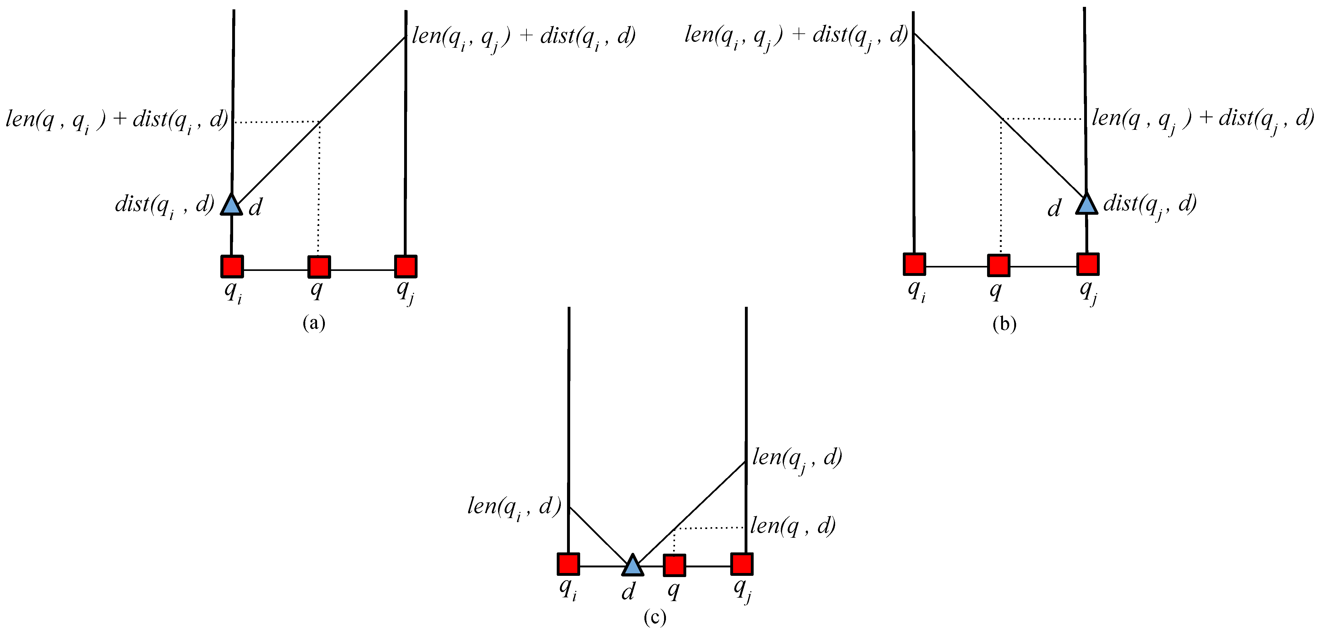
It is required to find the distance from the query object $q\in \overline{q_i{q}_j}$ to the nearest data object d. In Figure 4, $XY$ coordinates represent the distance and length from the query points to the data objects. X coordinate refers to the $len\left(q_i,q_j\right)$, whereas the Y coordinate refers to the distance from query point to data object $dist\left(q,d\right)$. When there exists a path from $q\to q_i\to d$, then, $dist\left(q,d\right)=len\left(q,q_i\right)+dist\left(q_i,d\right)$ is used to compute the distance. Likewise, if there exists a path from $q\to q_j\to d$, then $dist\left(q,d\right)=len\left(q,q_j\right)+dist\left(q_j,d\right)$ is used. Lastly, if the data object d exists inside of the $\overline{q_i{q}_j}$ then $dist\left(q,d\right)$ is evaluated as $dist\left(q,d\right)=len\left(q,d\right)$. Finally, from the array holding the computed distance, only the minimum distance is extracted as given below. Here, $len$ and $dist$ represent length and distance, respectively.

$$\begin{array}{c}\hfill dist\left(q,d\right)=\left\{\begin{array}{cc}min\left\{len\left(q,q_i\right)+dist\left(q_i,d\right),len\left(q,q_j\right)+dist\left(q_j,d\right)\right\},if d\notin \overline{q_i{q}_j}& \\ min\left\{len\left(q,q_i\right)+dist\left(q_i,d\right),len\left(q,q_j\right)+dist\left(q_j,d\right),len\left(q,d\right)\right\},otherwise\end{array}\right\}\end{array}$$

(1)

Table 2. Evaluation of $dist(q,d)$ for $q\in \overline{q_i{q}_j}$ and $d\in D^{q_i}\cup D^{q_j}\cup D\left(\overline{q_i{q}_j}\right)$.

Condition	dist(q,d)
$d\in D^{q_i}\cap D^{q_j}\cap D\left(\overline{q_i{q}_j}\right)$	$dist\left(q,d\right)=min\left\{len\left(q,q_i\right)+dist\left(q_i,d\right),len\left(q,q_j\right)+dist\left(q_j,d\right),len\left(q,d\right)\right\}$
$d\in D^{q_i}\cap D^{q_j}-D\left(\overline{q_i{q}_j}\right)$	$dist\left(q,d\right)=min\left\{len\left(q,q_i\right)+dist\left(q_i,d\right),len\left(q,q_j\right)+dist\left(q_j,d\right)\right\}$
$d\in D^{q_i}\cap D\left(\overline{q_i{q}_j}\right)-D^{q_j}$	$dist\left(q,d\right)=min\left\{len\left(q,q_i\right)+dist\left(q_i,d\right),len\left(q,d\right)\right\}$
$d\in D^{q_j}\cap D\left(\overline{q_i{q}_j}\right)-D^{q_i}$	$dist\left(q,d\right)=min\left\{len\left(q,q_j\right)+dist\left(q_j,d\right),len\left(q,d\right)\right\}$
$d\in D^{q_i}-\left(D^{q_j}\cup D\left(\overline{q_i{q}_j}\right)\right)$	$dist\left(q,d\right)=len\left(q,q_i\right)+dist\left(q_i,d\right)$
$d\in D^{q_j}-\left(D^{q_i}\cup D\left(\overline{q_i{q}_j}\right)\right)$	$dist\left(q,d\right)=len\left(q,q_j\right)+dist\left(q_j,d\right)$
$d\in D\left(\overline{q_i{q}_j}\right)-\left(D^{q_i}\cup D^{q_j}\right)$	$dist\left(q,d\right)=len\left(q,d\right)$

shows the conditions to compute the distance from the q to d. A data object can belong either to $D^{q_i}$, $D^{q_j}$, or $D\left(\overline{q_i{q}_j}\right)$. Retrieving the closest data object from $D^{q_i}\left(D^{q_j}\right)$ is more significant than retrieving the set of data objects from $D\left(\overline{q_i{q}_j}\right)$. The process of identifying the nearest-neighbor pairs is described in Algorithm 2. The shared execution process can be implemented to improve the execution time. 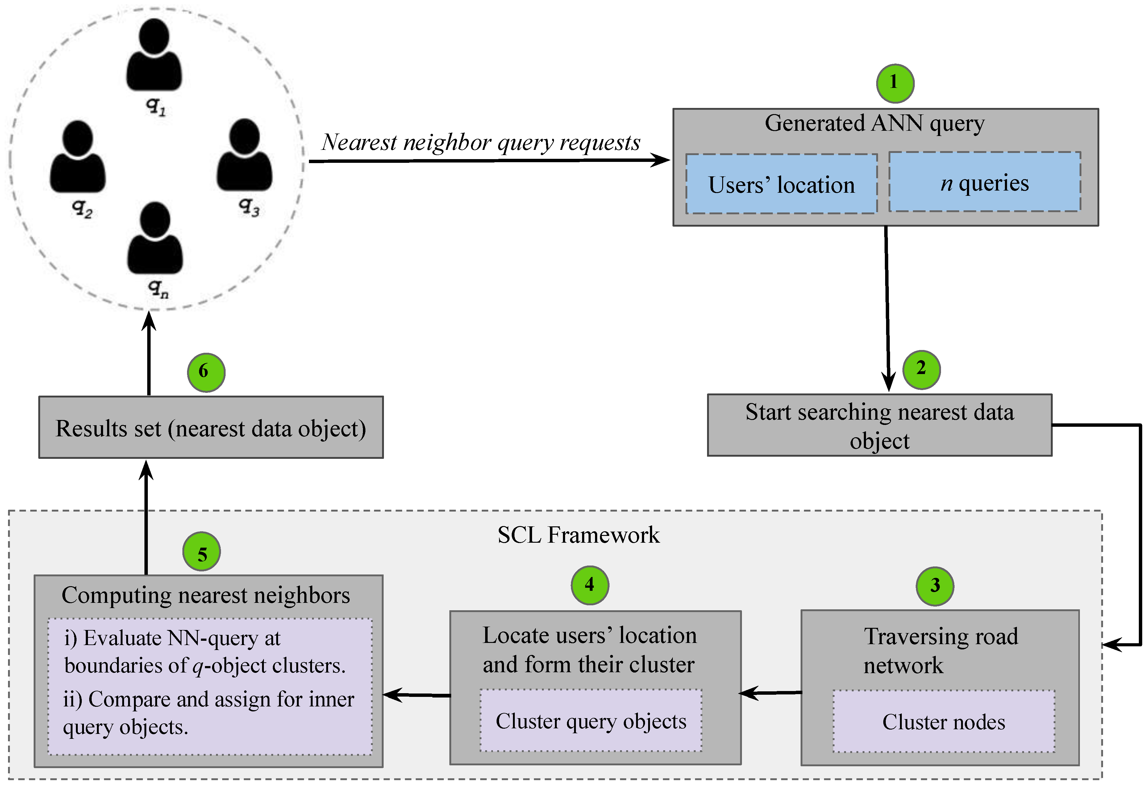Firstly, $\overline{\Omega }$, i.e., the set of object pairs, is initially assigned to be null. The algorithm comprises two steps. In the first step, the adjacent query objects are clustered together and query object clusters are formed and Q is transformed to $\overline{Q}$. The latter step involves the evaluation of the nearest neighbor query at the query object cluster $\overline{q_i{q}_j}$ to retrieve the nearest data object d.

Algorithm 2: SCL_Algorithm $\left(Q,D\right)$

The algorithm involves three different cases considering the number of query objects located in query object clusters. Case-I: $\left|\overline{q_i{q}_j}\right|=1$; Case-II: $\left|\overline{q_i{q}_j}\right|=2$; and Case-III: $\left|\overline{q_i{q}_j}\right|⩾3$. In Case-I, the NN query $NN\_Query\left(q_i\right)$ is evaluated at $q_i$, as in this case, the query object cluster $\overline{q_i{q}_j}$ consists solely of $q_i$. Following this, the NN query result is added to the partial join result $\overline{\Omega }\left(q_i\right)$ in $Lines$ 8–12. If it is Case-II, $NN\_Query\left(q_i\right)$ and $NN\_Query\left(q_j\right)$ are evaluated at $q_i$ and $q_j$, respectively. Then, the partial join result $\overline{\Omega }\left(q_i\right)$ and $\overline{\Omega }\left(q_j\right)$ are obtained, and the union is performed for the obtained partial sets, i.e., $\overline{\Omega }\left(q_i\right)\cup \overline{\Omega }\left(q_j\right)$ in $Lines$ 13–19.

Finally, for Case-III, two NN queries are evaluated, and the search for the nearest data objects is performed at $q_i$ and $q_j$. For each query object $q\in \left\{q_{i+1}\dots q_{j-1}\right\}$, the set of nearest neighbors of q is extracted in $Lines$ 12–24. According to Lemma 1, a partial join result $\overline{\Omega }\left(q_i{q}_j\right)$ can be extracted from $D^{q_i}\cup D^{q_i}\cup D\left(\overline{q_i{q}_j}\right)$ by applying the shared execution method. Finally, the join result set is obtained and the union of partial join results $\overline{\Omega }\left(q_i\right)\cup \overline{\Omega }\left(q_{i+1}\right)\cup \dots \overline{\Omega }\left(q_j\right)$ is returned in $Lines$ 25–29 after processing the entire query object cluster.

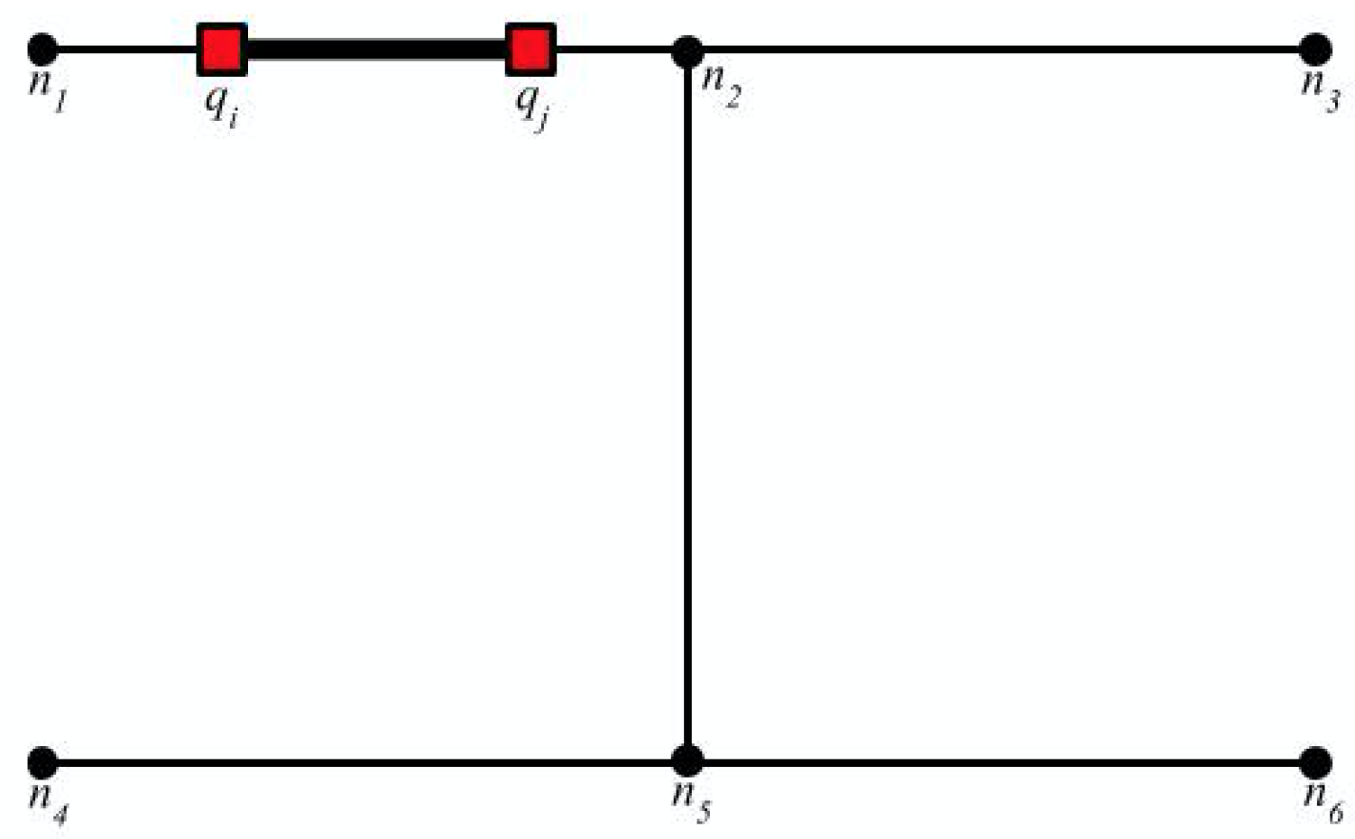
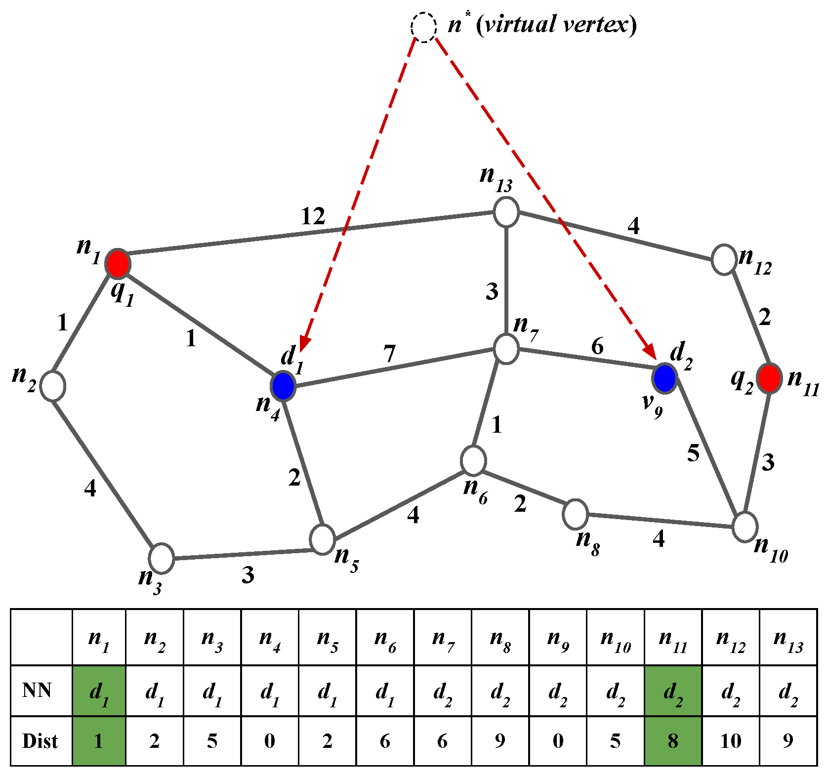
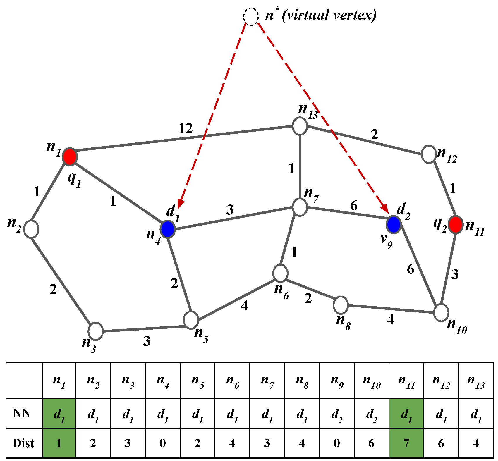
To bypass evaluating the redundant NN queries, a simple heuristic has been adopted, where no NN query is computed at query points close to the terminal nodes. For instance, as depicted in Figure 5, the graph consists of an intersection node $n_2$ with a query cluster $q_i{q}_j$ adjacent to it that ends with a terminal node $n_1$. In this example, the NN query at $q_i$ is unnecessary because it holds that $D^q\subseteq D^{q_j}\cup D\left(\overline{n_2{q}_j}\right)$, and it is sufficient to evaluate NN query at $\left\{q_j\right\}$.

5.2. Evaluation of SCL

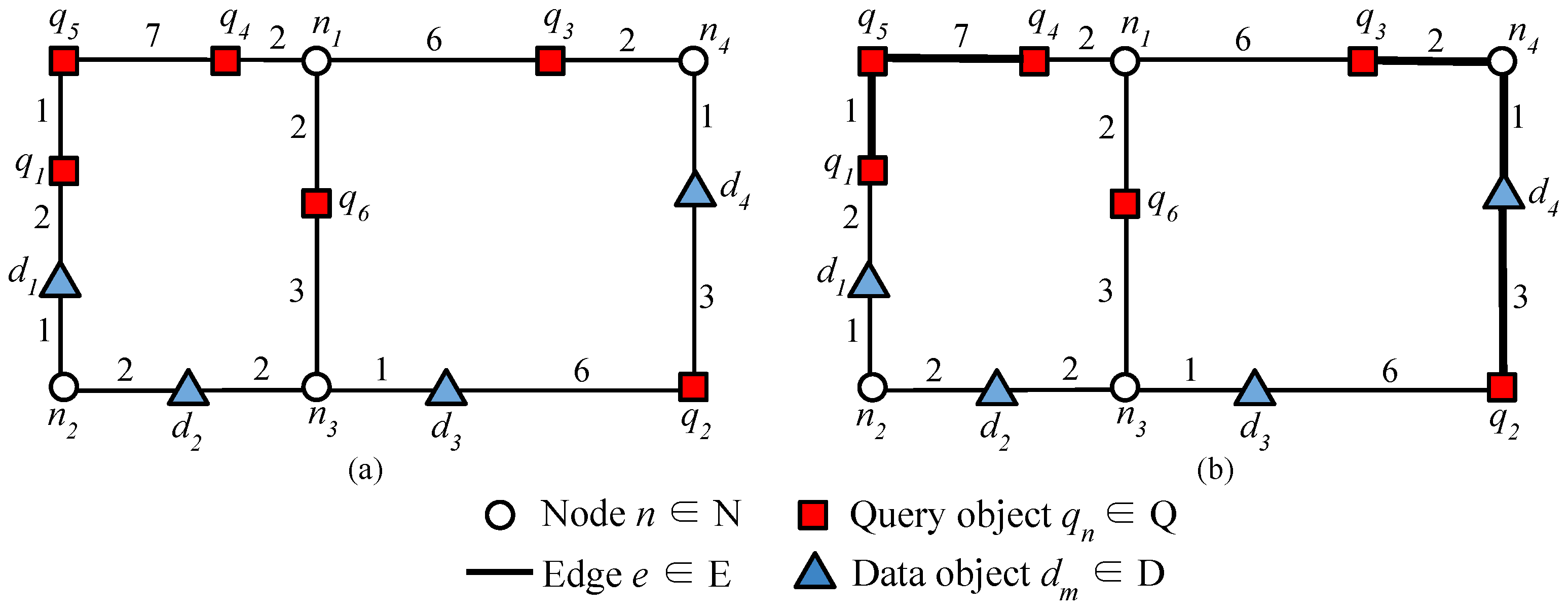
In this section, a brief discussion about the SCL algorithm has been carried out using Figure 3. Considering that, $Q=\left\{q_1,q_2,q_3,q_4,q_5,q_6\right\}$ and $D=\left\{d_1,d_2,d_3,d_4\right\}$ are the given sets of query and data objects, respectively. Query objects from Q have been clustered into query object clusters $\left(\overline{q_1{q}_5{q}_4}\right)$, $\left(\overline{q_3{q}_2}\right)$, and $\overline{q_6}$, all of which belong to $\overline{Q}$, as depicted in Figure 3b.

While processing $\overline{q_1{q}_5{q}_4}$ containing $q_1$, $q_5$, and $q_4$, the two NN queries are evaluated at $q_1$ and $q_4$ and the corresponding nearest data objects are retrieved. After evaluating the NN queries at two ends of the query object cluster, $D^{q_1}$ = $\left\{d_1\right\}$, $D^{q_4}$ = $\left\{d_3\right\}$, and $D\left(\overline{q_1{q}_5{q}_4}\right)$ = ⌀ are obtained. The simple partial join result sets can be generated based on this information as $\overline{\Omega }\left(q_1\right)$ = $\left\{〈q_1,d_1〉\right\}$ and $\overline{\Omega }\left(q_4\right)$ = $\left\{〈q_4,d_3〉\right\}$. Instead of evaluating the NN query corresponding to $q_5$, as it is an inner query object in the query object cluster $\overline{q_1{q}_5{q}_4}$. Rather, simply applying Lemma 1 is enough to retrieve the NN for $q_5$ based on the relation $D^{q_1}\cup D^{q_4}\cup D\left(\overline{q_1{q}_5{q}_4}\right)$ = $\left\{d_1,d_3\right\}$. 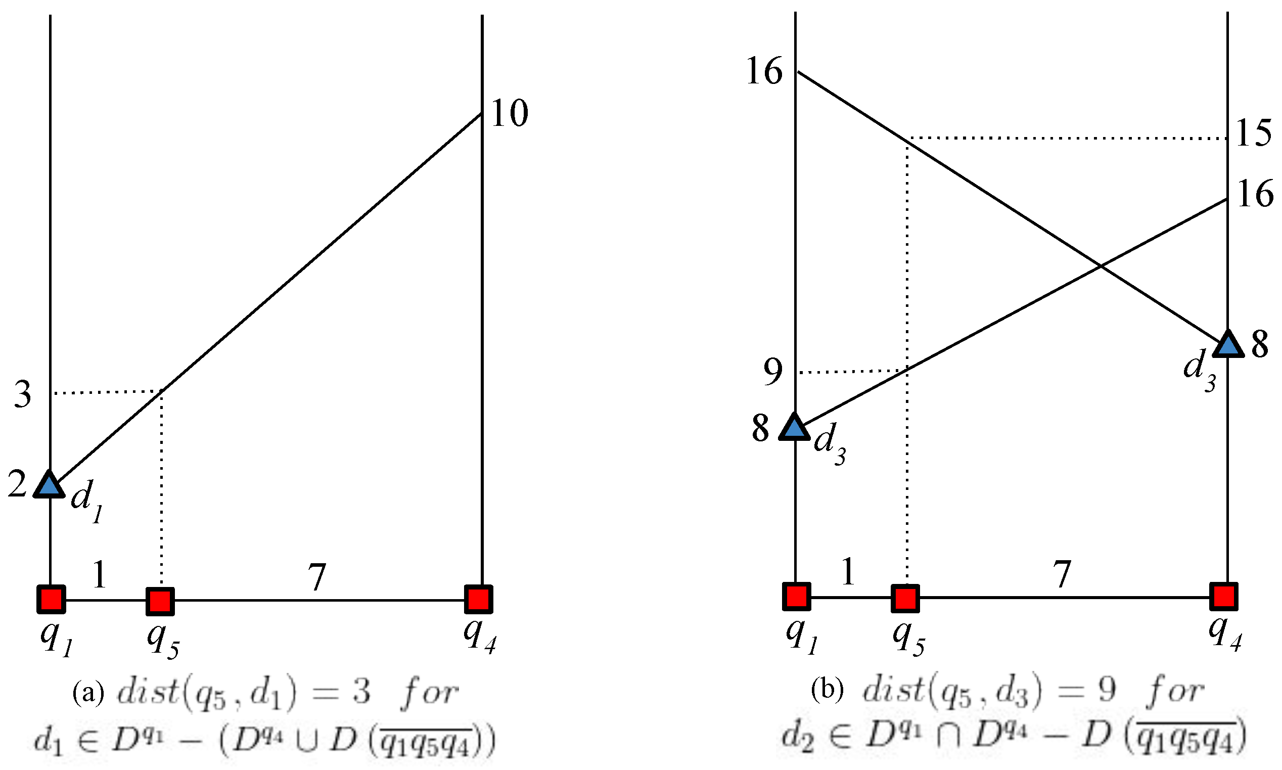For this purpose, it is necessary to compute the distance between $q_5$ and the candidate data object $d\in \left\{d_1,d_3\right\}$. It is evident that $d_1\in D^{q_1}\cup D^{q_4}-D\left(\overline{q_1{q}_5{q}_4}\right)$ and so, based on

Table 3. Computation of nearest neighbor $Q\bowtie D$ using the SCL method.

$\overline{{\mathit{q}}_{\mathit{i}}{\mathit{q}}_{\mathit{j}}}$	${\mathit{q}}_{\mathit{i}}$	${\mathit{q}}_{\mathit{j}}$	${\mathit{D}}^{{\mathit{q}}_{\mathit{i}}}$	${\mathit{D}}^{{\mathit{q}}_{\mathit{j}}}$	$\mathit{D}\left(\overline{{\mathit{q}}_{\mathit{i}}{\mathit{q}}_{\mathit{j}}}\right)$	$\left\{{\mathit{q}}_{\mathit{i}+1}\mathit{\dots }{\mathit{q}}_{\mathit{j}-1}\right\}$	${\mathit{D}}^{{\mathit{q}}_{\mathit{i}}}\cup {\mathit{D}}^{{\mathit{q}}_{\mathit{i}}}\cup \mathit{D}\left(\overline{{\mathit{q}}_{\mathit{i}}{\mathit{q}}_{\mathit{j}}}\right)$
$\overline{q_1{q}_5{q}_4}$	$q_1$	$q_4$	$\left\{d_1\right\}$	$\left\{d_2\right\}$	$D\left(\overline{q_1{q}_5{q}_4}\right)$ = ⌀	$\left\{q_5\right\}$	$\left\{d_1,d_2\right\}$
$\overline{q_2{q}_3}$	$q_2$	$q_3$	$\left\{d_4\right\}$	$\left\{d_4\right\}$	$D\left(\overline{q_2{q}_3}\right)$ = $d_4$	⌀	irrelevant
$q_6$	$q_6$	$q_6$	$\left\{d_3\right\}$	$\left\{d_3\right\}$	$D\left(q_6\right)$ = ⌀	⌀	irrelevant

, the distance between $q_5$ and $d_1$ is given by $dist\left(q_5,d_1\right)$ = $len\left(q_5,q_1\right)+dist\left(q_1,d_1\right)$ = 3, as depicted in Figure 6a. Similarly, $d_3\in D^{q_1}\cup D^{q_4}-D\left(\overline{q_1{q}_5{q}_4}\right)$ and so, based on Table 3, the distance from $q_5$ to $d_3$ is $dist\left(q_5,d_3\right)=min\left\{len\left(q_5,q_1\right)+dist\left(q_1,d_3\right),len\left(q_5,q_4\right)+dist\left(q_4,d_3\right)\right\}=min\left\{9,15\right\}$, as shown in Figure 6b.

Next, the evaluation of the NN queries at query object cluster $\overline{q_2{q}_3}$ is performed. As the query object cluster consists of only two query objects, the NN queries corresponding to both query objects need to be evaluated. On retrieving the set of the nearest data objects, the respective partial join result set is generated for each query object. From Table 3, it is observed that $D^{q_2}$ = $\left\{d_4\right\}$ and $D^{q_3}$ = $\left\{d_4\right\}$, then the partial join result set for $q_2$ and $q_3$ will be $\overline{\Omega }\left(q_2\right)$ = $\left\{\langle q_2,d_4\rangle \right\}$ and $\overline{\Omega }\left(q_3\right)$ = $\left\{\langle q_3,d_4\rangle \right\}$, respectively.

On successful processing, the NN queries from $\overline{q_2{q}_3}$, which leads to the final query point $q_6$. In this case, a single NN query is generated at $q_6$ and the partial join set for $q_6$ is performed as $\overline{\Omega }\left(q_6\right)$ = $\left\{\langle q_6,d_3\rangle \right\}$. Finally, the union of all query object clusters is computed to be $\overline{\Omega }\left(\overline{q_1{q}_5{q}_4}\right)\cup \overline{\Omega }\left(\overline{q_2{q}_3}\right)\cup \overline{\Omega }\left(q_6\right)$ = $\left\{〈q_1,d_1〉,〈q_4,d_3〉,〈q_5,d_1〉,〈q_2,d_4〉,〈q_3,d_4〉,〈q_6,d_3〉\right\}$ where $\overline{\Omega }\left(\overline{q_1{q}_5{q}_4}\right)$ = $\overline{\Omega }\left(q_1\right)\cup \overline{\Omega }\left(q_5\right)\cup \overline{\Omega }\left(q_4\right)$, and $\overline{\Omega }\left(\overline{q_2{q}_3}\right)$ = $\overline{\Omega }\left(q_2\right)\cup \overline{\Omega }\left(q_3\right)$, respectively.

5.3. Complexity Analysis

The complexity of finding the ANN queries using the proposed SCL method is covered as follows. The number of data objects are denoted as $\left|D\right|$, the number of query objects as $\left|Q\right|$, and the node cluster as $\overline{N}$. The number of nodes and edges are denoted as $\left|N\right|$ and $\left|E\right|$, respectively.

The clustering process takes $\mathcal{O}\left(\right|N|+\left|E\right|)+\mathcal{O}\left(\overline{N}\right)=\mathcal{O}\left(\right|N|+\left|E\right|+\overline{N})$. Initially, the road network is traversed from the terminal or intersection node until it reaches another intersection node. For the road network traversal, the SCL algorithm adopts a breadth-first search traversal with the worst-case time complexity of $\mathcal{O}\left(\right|N|+|E\left|\right)$. Once the node clustering is completed, the algorithm linearly scans through the node clusters to find query objects located in those node clusters. The scanning takes the linear search of $\mathcal{O}\left(\overline{N}\right)$ time.

The query time complexity of the SCL algorithm depends upon the number of query object clusters, i.e., $\overline{\left|Q\right|}$. At most, two NN queries are applied for each query object cluster that makes $2\times |\overline{Q}|$. To find the shortest path from the end of each query object cluster to the nearest data object, Dijkstra’s algorithm was implemented, which has a worst-case time complexity of $\mathcal{O}\left(\right|N|+|E\left|log\right|N\left|\right)$. Therefore, the time complexity of the SCL algorithm is expressed as: $\mathcal{O}\left(|\overline{Q}|\times \left(\left|N\right|+\left|E\right|log\left|N\right|\right)\right)$.

6. Experimental Evaluation

This section introduces an experimental approach to the algorithm analysis. Further, it is subdivided into a description of the experimental environment and the presentation of the results followed by the discussions.

6.1. Experimental Setup

Real road datasets from California, San-Joaquin, and Oldenburg, available in [35], were used to verify the performance of the proposed algorithm. The California dataset comprised 21,048 nodes and 21,693 edges, the San-Joaquin dataset comprised 18,263 nodes and 23,784 edges, and the Oldenburg dataset comprised 6105 nodes and 7035 edges. Further details about the datasets have been presented in

Table 4. Real-world roadmaps indicating attributes like nodes and edges. Node clusters and intermediate nodes are used later in the discussion section.

Code	Name	Nodes	Edges	Node Clusters	Intermediate Nodes
CAL	California	21,048	21,693	2010	19,683
SANJ	San Joaquin	18,623	23,784	19,929	3868
OLDEN	Oldenburg	6105	7035	3797	3232

.

The proposed SCL algorithm was employed in this study to find the NN queries on the disclosed datasets. In this paper, the query and data objects were assumed to move continuously in dynamic road networks, where the weights of the road segment (transit times and distances) were frequently updated and the distance between two objects was taken to be the length of the shortest path connecting them. ANN queries were taken to be snapshot-based rather than continuous queries. This required the system to store the current locations of the query and data objects. Thus, the movement of the query and data objects was not of much significance to the proposed method, as the frequent updates of network distance simply paralyzed the precomputed structures.

In each experiment, the size of data and query objects were changed. When the size of data objects was increased, then the size of the query object was kept static and vice-versa. The setup parameters used for this experiment are shown in

Table 5. Experimental parameters.

Parameter	Values
Number of data objects	2, 3, 5, 7, 10 $\left(\times {10}^4\right)$.
Number of query objects	2, 3, 5, 7, 10 $\left(\times {10}^4\right)$.
Distribution of query objects	(C)entroid, (U)niform
Distribution of data objects	(C)entroid, (U)niform
Real-world roadmaps	CAL, SANJ, OLDEN

. The bold values represent the default selected values throughout the experiments. Initially, 10 centroid datasets were generated that followed a Gaussian distribution, and the mean was set to the centroid, whereas the standard deviation was set to 2% of the side-length. The distribution of the query and data objects were taken to follow the centroid distribution, unless stated otherwise.

For the implementation and evaluation of the proposed scheme, the VIVET [18] and INE [21] algorithms were employed to compute the nearest data object for all n given query objects. The VIVET algorithm uses a lookup array table. Initially, it computes the distance from the virtual node and passes through every data object until it reaches the nearest node. Once it finds the nearest node, the distance table is updated, and a new distance is recorded in the lookup array table, whereas the INE algorithm starts the traversal from each query object and terminates the search once it finds the nearest data object. The three algorithms were implemented using Java language and run on a desktop PC running Linux 64-bit OS with 16 GB RAM and a 32-cores Intel processor at 2.10 GHz. The experiments were repeated five times, and the obtained average values were recorded.

6.2. Experimental Results

Figure 7, Figure 8 and Figure 9 depict the comparison of the query processing time for CAL, SANJ, and OLDEN datasets for the INE, SCL, and VIVET algorithms, respectively. The size of the query object was set to be 50 K as default and the data object varied from 20 to 100 K and vice-versa when the size of the query object varied. Finally, the figures show the various data distribution combinations (i.e., $\left(C,C\right),\left(C,U\right),\left(U,C,\right),\left(U,U\right))$ for the query and data objects.

Figure 7a illustrates the effect of the data object size growth on query processing. The query processing time tends to grow with the number of data objects. However, the growth of the data object size has less impact on the efficiency of SCL and INE algorithms. In fact, the SCL exhibits six times better performance than the VIVET algorithm due to the reason that the query processing of the SCL algorithm is not affected by the change in the size of the data object. For VIVET, when the data object size increased, the algorithm had to spend 65% of the computation time traversing from the virtual node, passing through every data object to find the nearest node and keeping the index table up to date.

Figure 7b illustrates the effect of the query object size growth on query processing. The query processing time for all three algorithms increases with an increasing number of query objects. Clearly, the SCL algorithm is two and four times faster than INE and VIVET, respectively. Moreover, when the $\left|Q\right|$ = 100 K, the SCL required approximately 25 K NN queries evaluations. It is also observed from the figure that INE was faster than the VIVET—since the query objects followed a centroid distribution—so that INE quickly came up with an NN result with less network traversal. As expected, VIVET performed much worse than SCL and INE because it required checking all data objects if they affect the lookup table. Note that each data object and query object are treated as nodes in VIVET, which alters the actual node count after augmenting the original graph G.

Figure 7c depicts the effect on query processing while both the query and data objects followed the various data distribution combinations. It is clear that under various distribution settings, SCL outperformed both INE and VIVET algorithms. When the query objects and data objects are uniformly distributed the INE and SCL show similar performance. Nonetheless, the VIVET severely gets affected while the query and data objects are uniformly distributed since all the objects are sparely scattered such that all objects are widely far from each other.

Figure 8a depicts a comparison of INE, SCL, and VIVET query processing time with respect to the data object size. For the 20 and 30 K data object size, SCL and VIVET show distinctly similar query processing times. On increasing the data object size to 100 K, it was observed that the processing time of SCL declined due to the reason that clustering query object reduces the number of NN query computations and is not heavily affected by the number of data objects. At the same time, the query processing time for VIVET shows a slight increment since VIVET depends upon the size of the data objects. The excessive intersection among the edges occurred, causing the INE to expand the traversal to reach the nearest data object. However, with an increased number of data objects up to 70 K, a significant plummeting of query processing time is observed for INE.

Figure 8b compares INE, SCL, and VIVET performance with respect to the number of the query objects. It is evident that the number of NN queries required to be evaluated was drastically reduced by the proposed SCL algorithm compared to others. The SCL shows up to six times faster performance than INE since the SCL algorithm only required evaluating approximately 30 K NN queries when $\left|Q\right|$ = 100 K. When $\left|Q\right|$ was increased, INE required more iterations to compute the NN queries, and thus its processing time increased more rapidly than other methods.

Figure 8c shows that the SCL algorithm performed well on all tested combinations distributions except $\left(U,C\right)$ owing to the same reason as in the case of the CAL dataset. The result shows that the performance of the INE algorithm degenerated significantly because the INE had to traverse a long-distance path before it accessed the NN data object. However, all methods show a similar performance when the query object followed the centroid distribution, that is, $\left(C,U\right)$.

Figure 9a illustrates the impacts of data object size on INE, SCL, and VIVET performance. The result shows that the data object size has a less significant impact on SCL. This experiment result demonstrates a similar trend as in Figure 7a. On average, VIVET incurred 90% of the computation cost during the rebuilding process of the precomputation table.

Figure 9b shows the effect of query object increment on INE, SCL, and VIVET. When the size of $\left|Q\right|$ increased, the shared execution drastically reduced redundant NN query computations. In particular, the processing time required by the SCL algorithm was observed to be 67% and 90% less than that required by the INE and VIVET algorithms, respectively.

Figure 9c depicts the query processing time when the query and data objects followed various distributions. The SCL method outperformed the INE and VIVET algorithms for every distribution combination. However, as expected, VIVET performed much worse than the other two algorithms as it consumed almost 80% of the computation time on keeping the index table up to date.

7. Discussion

From the above experimental results, it can be inferred that there was a huge difference in query processing time when the size of query objects was fixed or changed. The proposed algorithm aims to reduce the cost of query computation while there is a huge number of query objects. The SCL algorithm was implemented in a central server that was responsible for handling a huge number of queries. Since the SCL algorithm utilized the shared-execution technique, it became dominant over INE [21] and the VIVET [18] algorithms. Moreover, extending this work to a distributed environment [30,36,37] is likely to reduce the computation cost much more significantly, which leads to a future research direction.

The goal of this study emphasized the processing of ANN queries in a dynamic road environment. For that, the beginning step requires clustering the whole map dataset and storing it in the server. Following, the previously clustered information is later used to re-cluster the query objects belonging to each cluster at a time $t_1$. It is known that the ANN query is a snapshot-based query, which requires the server to take the snapshot after $t_{i+1}$ time and re-cluster in order to evaluate further ANN queries. Figure 10 and Figure 11 show the performance improvement of the SCL algorithm over the INE and the VIVET algorithms in terms of query processing time on three different datasets—California (CAL), San Joaquin (SANJ), and Oldenburg (OLDEN)—while the size of query objects increase with two different distributions, i.e.,$\left(C,U\right)$ and $\left(U,U\right)$. As is evident in the aforementioned results, the SCL algorithm performs best when involving a large number of query objects. In addition, ANN queries are designed to cater to spatial query processing in the presence of a large number of query objects.

Figure 10 illustrates the initial performance of the proposed algorithm on all three datasets with respect to the INE, which starts from 40–60% and then drops almost to 7–22%. However, when increasing the size of the query objects, the performance is progressively regained up to 60% again. However, with the VIVET, the performance of the SCL starts from 42–82%, and then slightly drops in performance down to 50%. In the case when the size of query objects is less than data objects, the performance difference is significant, and as the query object size tends to grow, the performance gap increases.

From Figure 11, it can be interpreted that the initial performance of the SCL versus the INE on all three datasets starts from 7–14% and achieves a significant performance growth approximately up to 50% when the query object size is at 50K. As the size keeps on increasing, the performance again jumps down to almost 30%. The performance of the SCL with respect to the INE improves with the increment in the query object size. When the query objects were densely scattered, the shared execution process alleviated the processing time but when the query objects were widely scattered following a uniform distribution, the query processing time was aggravated for both INE and SCL algorithms.

In addition, it can be inferred that the query processing time for the VIVET shows a linear growth due to the fact that the query processing time depends upon the number of data objects. It is due to the reason that the VIVET algorithm was designed to process the ANN queries in a static road network and whenever the location update occurs, the ANN has to rebuild the index from the start. On the other hand, due to the shared execution processing, the number of NN queries evaluated by the SCL method decreased with an increase in the size of data objects. When the data objects are uniformly distributed, the time required for each data object to locate its nearest node is longer, which is the reason why the SCL performance improved with respect to the VIVET. VIVET performed worse as the size of query objects kept on increasing. This demonstrates that the SCL algorithm optimized the shared execution processing more effectively for large datasets.

As from Table 4, the ratios of intermediate nodes to the total number of nodes for all datasets were found to be ≈0.94, ≈0.21, and ≈0.53, respectively. This shows that when that ratio of intermediate nodes to the total number of nodes is close to 1.0, the performance of the SCL algorithm increases moderately. Another parameter to take into consideration could be a relation of the number of node clusters to the number of total nodes. The CAL dataset has many intermediate nodes that contribute to forming a few node clusters. However, for the SANJ dataset, the number of node clusters is greater than that of its total number of nodes. This also can be a contributing factor for a slight improvement of performance over the increase of query objects. To sum up, the SCL algorithm is up to six times faster than INE and VIVET, particularly when the query objects exhibit a centroid distribution. Secondly, the INE algorithm often outperforms VIVET clearly when the number of data objects is larger than 50,000. The performance study implies that the shared execution technique reduces the number of NN queries evaluation to process large query requests efficiently.

Limitations of VIVET in the Dynamic Road Network

Figure 12 and Figure 13 depict the precomputation and query lookup stages of the VIVET algorithm. In order to restrict overlapping network traversal and duplication of the computation, VIVET traverses the network starting from a virtual node $n^{*}$ that connects to all data objects. For each node $n_i$, there is always one data object $d_i$ on the shortest path from its virtual node such that $d_i$ is the nearest neighbor of the node $n_i$. Then the results are stored in a precomputation table that holds the N number of nodes. The VIVET algorithm assumes that data objects and query objects are located at the graph nodes. Once the precomputation is completed, the ANN query can answer the results by locating the node on which every query object $q_i$ lies and then return the nearest data object $d_i$ for that query object $q_i$.

The VIVET algorithm has been specifically designed to support the ANN query processing in a static road network. A precomputation table that holds the data object and the nearest node to each data object can be used to find the nearest query object. However, in a dynamic road network environment, the weight of an edge can be changed frequently, which invalidates the precomputed distance between query and data objects. Thus, in order to generate a valid query result, the precomputation table must be updated whenever there is a change in the network that significantly increases the computation overhead.

Figure 12 shows a precomputation table at time $t_1$. The NN results for two query objects $q_1$ and $q_2$ are shown in the green box. After traversing to all the vertices starting from the virtual node $n^{*}$ and passing through the connected data objects $d_1$ and $d_2$, the precomputation table is filled with the nearest neighbors of the nodes. The precomputation table is also known as $NNarray$. The shortest path connecting from $n^{*}$ to $q_1$ and $q_2$ passes through $\left\{n^{*}\to n_4\to n_1\right\}$ and $\left\{n^{*}\to n_9\to n_{10}\to n_{11}\right\}$ with the respective distance as one and eight. The green box shows the nearest neighbor for the query objects $q_1$ and $q_2$ lying on the nodes $n_1$ and $n_{11}$ as $d_1$ and $d_2$. Now let us consider, at time $t_{i+1}$ the weight of edges $\left(n_2,n_3\right),\left(n_4,n_7\right),\left(n_7,n_{13}\right),\left(n_{13},n_{12}\right),\left(n_{12},n_{11}\right)$, $\left(n_9,n_{10}\right)$ change due to certain traffic conditions. Then, the shortest path distance that connects $n^{*}$ to $n_{11}$ changes to $\left\{n^{*}\to n_7\to n_{13}\to n_{12}\to n_{11}\right\}$ with a distance of seven. When there occurs a change in network distance, the VIVET nullifies the $NNarray$ table; afterward, the traversal is initialized that recomputes the NN pairs, and finally, the NN array table is updated, which has been shown in Figure 13 and it also changes the NN result for $q_2$, which becomes $d_1$. Whenever there exists a huge number of road network updates that require fresh results, indexing techniques are less efficient as it poses computation overhead.

Table 6. Comparison of time and space complexities of INE, SCL, and VIVET.

	INE	SCL	VIVET
(1) Query Cost	$\left|Q\right|\times \mathcal{O}\left(\left|E\right|+\left|N\right|\times log\left|N\right|\right)$	$|\overline{Q}|\times \mathcal{O}\left(\left|E\right|+\left|N\right|\times log\left|N\right|\right)$	$\mathcal{O}\left(\left|Q\right|\right)$
(2) Precomputation Cost	$\mathcal{O}\left(1\right)$	$\mathcal{O}\left(1\right)$	$\mathcal{O}\left(\left(\left|E\right|+\left|N\right|+\left|D\right|\right)\times log\left|N\right|\right)$
Run-time Complexity (1 + 2)	$\left|Q\right|\times \mathcal{O}\left(\left|E\right|+\left|N\right|\times log\left|N\right|\right)$	$|\overline{Q}|\times \mathcal{O}\left(\left|E\right|+\left|N\right|\times log\left|N\right|\right)$	$\mathcal{O}\left(\left(\left|E\right|+\left|N\right|+\left|D\right|\right)\times log\left|N\right|\right)+\left|Q\right|$
Space Complexity	$\mathcal{O}\left(\left|Q\right|\right)$	$\mathcal{O}\left(|\overline{Q}|\right)$	$\mathcal{O}\left(\left|N\right|\right)$

shows the time and space complexities of the INE, SCL, and VIVET algorithms. The INE and SCL are almost identical when it comes to the ANN query lookup because both of the algorithms start traversing the road network from the query point and expanding the adjacent edges until it reaches its nearest neighbor data point. Thus, the input size for the INE and SCL are $\left|Q\right|$, and $|\overline{Q}|$, respectively. However, SCL reduces the number of query points by clustering them hence reducing the NN query evaluations. On the other hand, the ANN query lookup using VIVET is linear to the size of the query objects, i.e., $\left|Q\right|$. As mentioned earlier, INE and SCL do not use any precomputation technique; hence, maintaining an index is always $\mathcal{O}\left(1\right)$. On the other hand, VIVET purely adopts the light indexing scheme, and precomputed results are stored in an NN array lookup table; therefore, VIVET takes $\mathcal{O}\left(\left(\left|E\right|+\left|N\right|+\left|D\right|\right)\times log\left|N\right|\right)$ during the precomputation phase. Therefore, the run-time complexity of VIVET is $\mathcal{O}\left(\left(\left|E\right|+\left|N\right|+\left|D\right|\right)\times log\left|N\right|\right)+\left|Q\right|$. The total run-time taken by INE and SCL depends upon the size of the query points, but for VIVET, the data object size affects the run-time. In contrast, the SCL algorithm significantly reduces the number of query points by clustering them; hence, the size of $|\overline{Q}|$ will be relatively small than the size of $\left|D\right|$. To conclude, the VIVET inherently shows a worse performance in dynamic road networks than in static road networks because it has to perform precomputation whenever there is an update in the network distance.

8. Conclusions

Following, the analysis of the space complexities of the algorithms is carried out. The space complexity of the INE algorithm is $\mathcal{O}\left(\left|Q\right|\right)$ due to the reason that NN queries are evaluated from all existing query objects. The SCL takes $\mathcal{O}\left(|\overline{Q}|\right)$ because the existing number of query objects are first scanned, then clustered to form a query cluster and for every query cluster $|\overline{Q}|$, the memory consumption is 2$\times |\overline{Q}|$ since, at most, two NN queries are required for a query segment. The VIVET algorithm initially creates an augmented graph $G^{*}$ from an original graph G. During the augmentation process, all the query objects and data objects are transformed into nodes, such that data objects and query objects are on the nodes. Storing the additional number of nodes during the execution would take the space of $\mathcal{O}\left(\left|N\right|\right)$. Consequently, the memory consumption of the SCL is comparatively smaller than those of precomputed methods.

This study investigated efficient methods to process ANN queries in dynamic road networks. Specifically, ANN queries involve processing a huge number of query requests, which imposes a high computational burden. Therefore, this paper proposed an efficient framework to process ANN queries in a dynamic road network that reduces the computation cost. To enhance the efficiency and effectiveness of the proposed algorithm, the shared execution technique is adopted that initially creates a cluster of nodes, followed by clustering of query objects in order to bypass redundant NN evaluations.

To evaluate the performance of the proposed algorithm, a simulation experiment was conducted that used real-world road network maps. Various data distribution combinations were used to evaluate the performance of the proposed framework. With the experimental demonstrations, it was verified that the proposed algorithm outperforms the VIVET and INE algorithms. Further, the evidence from the results proved that the SCL algorithm performs best to evaluate queries in cases involving a large number of query objects in a road segment. Motivated by the limitations of this work, as mentioned in the discussion section, extending this approach to the problem of distributed query processing in dynamic road environments can be further studied. This could facilitate minimizing the wireless communication and the server computation costs, both of which are heavily dependent on the amount of the location-update stream generated by moving objects. Additionally, the prospect of being able to integrate the shared execution approach with Markov’s chain state model can support AI-based recommendation systems, which serve as a spur for future research.

References

1. Zhang, J.; Zhu, M.; Papadias, D.; Tao, Y.; Lee, D.L. Location-based spatial queries. In Proceedings of the 2003 ACM SIGMOD International Conference on Management of Data, San Diego, CA, USA, 10–12 June 2003; p. 443. [Google Scholar] [CrossRef] [Green Version]
2. Jung, H.; Song, M.; Youn, H.Y.; Kim, U.M. Evaluation of content-matched range monitoring queries over moving objects in mobile computing environments. Sensors 2015, 15, 24143–24177. [Google Scholar] [CrossRef] [PubMed] [Green Version]
3. Wan, S.; Zhao, Y.; Wang, T.; Gu, Z.; Abbasi, Q.H.; Choo, K.K.R. Multi-dimensional data indexing and range query processing via Voronoi diagram for internet of things. Future Gener. Comput. Syst. 2019, 91, 382–391. [Google Scholar] [CrossRef] [Green Version]
4. Mouratidis, K.; Yiu, M. Continuous nearest neighbor monitoring in road networks. In Proceedings of the 32nd International Conference on Very Large Data Bases, Seoul, Korea, 12–15 September 2006; pp. 43–54. [Google Scholar]
5. Cho, H.J.; Kwon, S.J.; Chung, T.S. A safe exit algorithm for continuous nearest neighbor monitoring in road networks. Mob. Inf. Syst. 2013, 9, 37–53. [Google Scholar] [CrossRef]
6. Attique, M.; Cho, H.J.; Jin, R.; Chung, T.S. Efficient processing of continuous reverse k nearest neighbor on moving objects in road networks. ISPRS Int. J. Geo-Inf. 2016, 5, 247. [Google Scholar] [CrossRef] [Green Version]
7. Attique, M.; Qamar, R.; Cho, H.J.; Chung, T.S. A new approach to process top-k spatial preference queries in a directed road network. In Proceedings of the Third ACM SIGSPATIAL International Workshop on Mobile Geographic Information Systems, Dallas, TX, USA, 4–7 November 2014; pp. 34–42. [Google Scholar]
8. Attique, M.; Cho, H.J.; Jin, R.; Chung, T.S. Top-k spatial preference queries in directed road networks. ISPRS Int. J. Geo-Inf. 2016, 5, 170. [Google Scholar] [CrossRef] [Green Version]
9. Attique, M.; Cho, H.J.; Chung, T.S. Efficient Processing of Moving Top-Spatial Keyword Queries in Directed and Dynamic Road Networks. In Wireless Communications and Mobile Computing; John Wiley and Sons: West Sussex, UK, 2018; Volume 2018. [Google Scholar]
10. Wang, H.; Zimmermann, R. Snapshot location-based query processing on moving objects in road networks. In Proceedings of the 16th ACM SIGSPATIAL International Conference on Advances in Geographic Information Systems, Irvine, CA, USA, 5–7 November 2008; pp. 403–406. [Google Scholar] [CrossRef]
11. Wang, H.; Zimmermann, R. A novel dual-index design to efficiently support snapshot location-based query processing in mobile environments. IEEE Trans. Mob. Comput. 2010, 9, 1280–1292. [Google Scholar] [CrossRef]
12. Cheema, M.A.; Zhang, W.; Lin, X.; Zhang, Y. Efficiently processing snapshot and continuous reverse k nearest neighbors queries. VLDB J. 2012, 21, 703–728. [Google Scholar] [CrossRef]
13. Priya, M.; Kalpana, R. Distributed processing of location based spatial query through vantage point transformation. Future Comput. Inform. J. 2018, 3, 296–303. [Google Scholar] [CrossRef]
14. Dong, T.; Yuan, L.; Shang, Y.; Ye, Y.; Zhang, L. Direction-aware continuous moving k-nearest-neighbor query in road networks. ISPRS Int. J. Geo-Inf. 2019, 8, 379. [Google Scholar] [CrossRef] [Green Version]
15. Zhang, M.; Li, L.; Hua, W.; Zhou, X. Typical Snapshots Selection for Shortest Path Query in Dynamic Road Networks. In Lecture Notes in Computer Science; Springer: Cham, Switzerland, 2020; Volume 12008, pp. 105–120. [Google Scholar] [CrossRef] [Green Version]
16. Clarkson, K.L. Fast algorithms for the all nearest neighbors problem. In Proceedings of the 24th Annual Symposium on Foundations of Computer Science (SFCS 1983), Tucson, AZ, USA, 7–9 November 1983; pp. 226–232. [Google Scholar] [CrossRef]
17. Zhang, J.; Mamoulis, N.; Papadias, D.; Tao, Y. All-nearest-neighbors queries in spatial databases. In Proceedings of the 16th International Conference on Scientific and Statistical Database Management, Chania, Greece, 25–27 June 2004; pp. 297–306. [Google Scholar] [CrossRef] [Green Version]
18. Xu, Y.; Qi, J.; Borovica-Gajic, R.; Kulik, L. Finding all nearest neighbors with a single graph traversal. In Proceedings of the International Conference on Database Systems for Advanced Applications, Gold Coast, Australia, 21–24 May 2018; Volume 10827, pp. 221–238. [Google Scholar] [CrossRef]
19. Amin, A.M.; Ali, M.E.; Hashem, T. Shared Execution of Path Queries on Road Networks. arXiv 2012, arXiv:1210.6746. [Google Scholar]
20. Mahmud, H.; Amin, A.M.; Ali, M.E. A Group Based Approach for Path Queries in Road Networks. In International Symposium on Spatial and Temporal Databases; Springer: Berlin/Heidelberg, Germany, 2013. [Google Scholar]
21. Papadias, D.; Zhang, J.; Mamoulis, N.; Tao, Y. Query Processing in Spatial Network Databases Dimitris. In Proceedings of the 2003 VLDB Conference, Morgan Kaufmann, Berlin, Germany, 9–12 September 2003; Volume 29. [Google Scholar]
22. Samet, H.; Sankaranarayanan, J.; Alborzi, H. Scalable network distance browsing in spatial databases. In Proceedings of the 2008 ACM SIGMOD International Conference on Management of Data, Vancouver, BC, Canada, 10–12 June 2008; pp. 43–54. [Google Scholar] [CrossRef] [Green Version]
23. Lee, K.C.; Lee, W.C.; Zheng, B.; Tian, Y. ROAD: A new spatial object search framework for road networks. IEEE Trans. Knowl. Data Eng. 2012, 24, 547–560. [Google Scholar] [CrossRef]
24. Zhong, R.; Li, G.; Tan, K.L.; Zhou, L.; Gong, Z. G-Tree: An Efficient and Scalable Index for Spatial Search on Road Networks. IEEE Trans. Knowl. Data Eng. 2015, 27, 2175–2189. [Google Scholar] [CrossRef]
25. Huang, X.; Jensen, C.S.; Lu, H.; Šaltenis, S. S-GRID: A versatile approach to efficient query processing in spatial networks. In International Symposium on Spatial and Temporal Databases; Springer: Berlin/Heidelberg, Germany, 2007; Volume 4605, pp. 93–111. [Google Scholar] [CrossRef]
26. Jensen, C.S.; Kolář, J.; Pedersen, T.B.; Timko, I. Nearest neighbor queries in road networks. In Proceedings of the 11th ACM International Symposium on Advances in Geographic Information Systems, New Orleans, LA, USA, 7–8 November 2003; pp. 1–8. [Google Scholar] [CrossRef] [Green Version]
27. Cho, H.J.; Chae, J. A safe exit algorithm for moving k nearest neighbor queries in directed and dynamic spatial networks. J. Inf. Sci. Eng. 2016, 32, 969–993. [Google Scholar]
28. Nannicini, G.; Baptiste, P.; Barbier, G.; Krob, D.; Liberti, L. Fast paths in large-scale dynamic road networks. Comput. Optim. Appl. 2010, 45, 143–158. [Google Scholar] [CrossRef] [Green Version]
29. Xu, J.; Gao, Y.; Liu, C.; Zhao, L.; Ding, Z. Efficient route search on hierarchical dynamic road networks. Distrib. Parallel Databases 2015, 33, 227–252. [Google Scholar] [CrossRef]
30. Zhang, D.; Yang, D.; Wang, Y.; Tan, K.L.; Cao, J.; Shen, H.T. Distributed shortest path query processing on dynamic road networks. VLDB J. 2017, 26, 399–419. [Google Scholar] [CrossRef]
31. Huang, X.; Chen, D.; Wang, D.; Ren, T. MINE: Identifying Top-k Vital Nodes in Complex Networks via Maximum Influential Neighbors Expansion. Mathematics 2020, 8, 1449. [Google Scholar] [CrossRef]
32. Oehlers, M.; Fabian, B. Graph Metrics for Network Robustness—A Survey. Mathematics 2021, 9, 895. [Google Scholar] [CrossRef]
33. Gibbons, A. Algorithmic Graph Theory; Cambridge University Press: Cambridge, UK, 1985. [Google Scholar]
34. Cho, H.J. Efficient Shared Execution Processing of k-Nearest Neighbor Joins in Road Networks. Mob. Inf. Syst. 2018, 2018. [Google Scholar] [CrossRef] [Green Version]
35. Real Datasets for Spatial Databases. Available online: https://www.cs.utah.edu/~lifeifei/SpatialDataset.htm (accessed on 15 May 2021).
36. Wang, H.; Zimmermann, R. Processing of continuous location-based range queries on moving objects in road networks. IEEE Trans. Knowl. Data Eng. 2011, 23, 1065–1078. [Google Scholar] [CrossRef]
37. Jung, H.R.; Kim, U.M. The SSP-Tree: A method for distributed processing of range monitoring queries in road networks. ISPRS Int. J. Geo-Inf. 2017, 6, 322. [Google Scholar] [CrossRef] [Green Version]
Figure 1. Example of dynamic road network (a) traffic condition at time t 1 ; (b) traffic condition at time t 2 where, Q = q 1 , q 2 , q 3 , q 4 , q 5 and D = d 1 , d 2 , d 3 , d 4 .
Mathematics 09 01137 g001
Figure 2. Workflow diagram of the proposed query processing methodology.
Mathematics 09 01137 g002
Figure 3. Initial Road network, and road network after clustering query objects, query object clusters are denoted by the bold lines (a) Nodes Clustering; (b) Query Objects Clustering.
Mathematics 09 01137 g003
Figure 4. Conditions to compute the distance from q to d: (a) If d D q i , then d i s t q i , d = l e n q , q i + d i s t q i , d ; (b) If d D q j , then d i s t q j , d = l e n q , q j + d i s t q j , d ; (c) If d q i q j ¯ , then d i s t q , d = l e n q , d .
Mathematics 09 01137 g004
Figure 5. Heuristic D q D q j D n 2 q j ¯ for each query segment q q i q j ¯ .
Mathematics 09 01137 g005
Figure 6. Computing distance from q 5 to d d 1 , d 3 .
Mathematics 09 01137 g006
Figure 7. Comparison of INE, SCL, and VIVET for CAL: (a) varying D; (b) varying Q; (c) varying the distribution of objects.
Mathematics 09 01137 g007
Figure 8. Comparison of INE, SCL, and VIVET for SANJ: (a) varying D; (b) varying Q; (c) varying the distribution of objects.
Mathematics 09 01137 g008
Figure 9. Comparison of INE, SCL, and VIVET for OLDEN: (a) varying D; (b) varying Q; (c) varying the distributionof objects.
Mathematics 09 01137 g009
Figure 10. Performance improvement by increasing the query object size following C , U distribution.
Mathematics 09 01137 g010
Figure 11. Performance improvement by increasing the query object size following U , U distribution.
Mathematics 09 01137 g011
Figure 12. An example of VIVET at t 1 , the green box indicates the query results.
Mathematics 09 01137 g012
Figure 13. An example of VIVET at t i + 1 with updated distances, the green box indicates the query results.
Mathematics 09 01137 g013