Reliability Properties of the NDL Family of Discrete Distributions with Its Inference

Abstract

The natural discrete Lindley (NDL) distribution is an intuitive idea that uses discrete analogs to well-known continuous distributions rather than using any of the published discretization techniques. The NDL is a flexible extension of both the geometric and the negative binomial distributions. In the present article, we further investigate new results of value in the areas of both theoretical and applied reliability. To be specific, several closure properties of the NDL are proved. Among the results, sufficient conditions that maintain the preservation properties under useful partial orderings, convolution, and random sum of random variables are introduced. Eight different methods of estimation, including the maximum likelihood, least squares, weighted least squares, Cramér–von Mises, the maximum product of spacing, Anderson–Darling, right-tail Anderson–Darling, and percentiles, have been used to estimate the parameter of interest. The performance of these estimators has been evaluated through extensive simulation. We have also demonstrated two applications of NDL in modeling real-life problems, including count data. It is worth noting that almost all the methods have resulted in very satisfactory estimates on both simulated and real-world data.

1. Introduction

Interests in discrete failure data came relatively late in comparison to its continuous analog. The subject matter has, to some extent, been neglected. It was only briefly mentioned by [1]. For earlier works on discrete lifetime distributions, see [2,3,4,5]. In the last few decades, many papers have appeared in the statistical literature on the discretization of continuous distributions. The most recent discrete distributions include the discrete analogs of the continuous Burr and Pareto distributions [6], discrete analog of the continuous inverse Weibull distribution [7], and discrete analog of the generalized exponential distribution [8]. These three distributions have at least two parameters each and have not yet received any applications. Further, the moments of the three distributions are expressed in terms of either non-standard special functions or infinite sums.

In spite of all the available discrete models, there is still a great need to create more flexible discrete distributions to model several types of real data in many applied areas, such as social sciences, economics, biometrics, and reliability studies, to model different types of count data.

Recently, Al-Babtain et al. [9] introduced the natural discrete Lindley (NDL) distribution, using a mixture of geometric and negative binomial distributions. However, the authors saw that there was still a lot of room for introducing new results relating the NDL to both theoretical and applied reliability, which has motivated the authors to further study the NDL distribution.

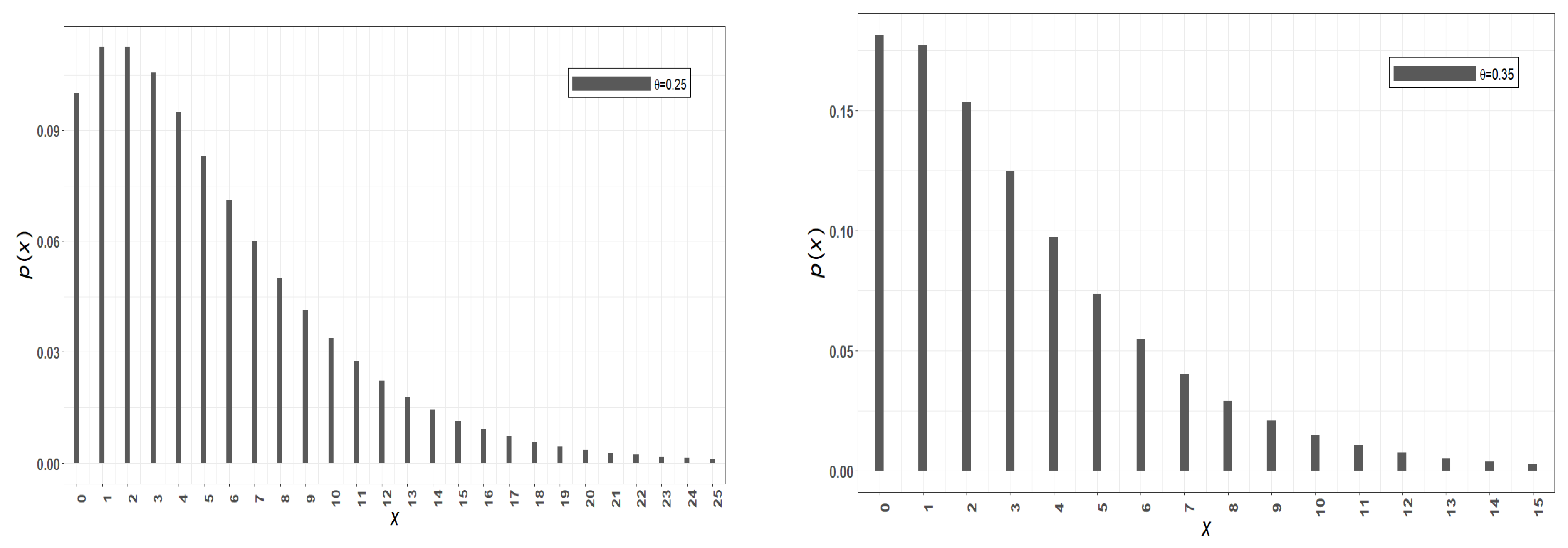
The NDL distribution [9], specified by the probability mass function (PMF), is

$$p\left(x\right)=\frac{{\theta }^2}{1+\theta }\left(2+x\right){\left(1-\theta \right)}^x, x=0, 1, 2,\dots \mathrm{and} \theta \in \left(0,1\right),$$

where survival function (SF) and hazard rate (HR) function are, respectively, given by

$$S\left(x\right)=P\left(X\ge x\right)=\frac{1+\theta +\theta x}{1+\theta }{\left(1-\theta \right)}^x, x=0,1,2,\dots \mathrm{and} \theta \in \left(0,1\right)$$

and

$$r\left(x\right)=\frac{p\left(x\right)}{P\left(X\ge x\right)}=\frac{{\theta }^2\left(2+x\right)}{1+\theta +\theta x}, x=0,1,2,\dots \mathrm{and} \theta \in \left(0,1\right).$$

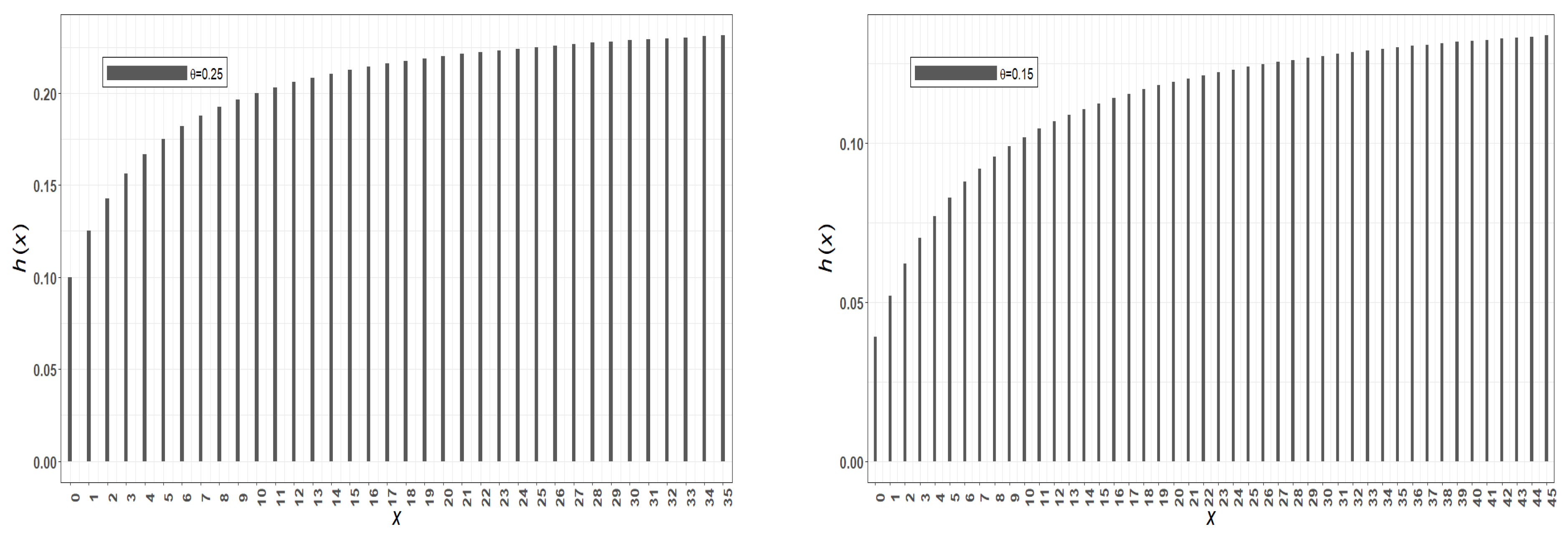
Further details about the NDL distribution can be explored in [9]. For example, Figure 1 and Figure 2 display possible shapes for the PMF and HR function of the NDL distribution for some values of $\theta$, to show that the NDL distribution is always uni-modal for all values of $\theta \in \left(0, 1\right)$, whereas its HR function is always increasing in $\theta$.

In the current article, several additional theoretical reliability properties, as well as useful partial orderings, are introduced. Besides, different methods for estimating the involved parameter are explored, and their results compared.

Among the basic results, it has been shown that the hazard rate ordering of members of the NDL family is preserved under a common contamination. This is quite useful in the case where the systems are operating under random common environments. Important results are derived covering the preservation of the sums of random variables under the hazard rate, likelihood ratio, and the reversed hazard rate. Such results are quite useful in the reliability practicing. More importantly, it is shown that the life lengths of two series systems composed of ordered components of the NDL family preserve the hazard rate order. A basic result gives sufficient conditions for the preservation of the D-MRL property under the assumption of log-concavity of an added contamination. Other, similar results consider the D-MRL case. Finally, an interesting application to renewal processes, which is very helpful in “replacement studies”, is also presented.

In particular, we give sufficient conditions that maintain the preservation properties under useful partial orderings, convolution, and random sum of random variables. Preservation under common random effects of the surrounding environment is also established. Moreover, interesting applications to weighted distributions and length-biased models have been carefully investigated. Finally, different methods have been used to estimate the parameter of the NDL, and the efficiencies of these estimation methods have been compared.

The rest of the paper is organized as follows. For completeness, several reliability closure properties and useful partial ordering comparisons are established in Section 2. In Section 3, a discrete renewal process application is presented. Section 4 is devoted to inferences about the involved parameter. In Section 5, we conduct a detailed simulation study to explore the behavior of the proposed estimators. In Section 6, the validity of estimation methods is checked empirically using two real biological datasets. Finally, conclusions and future work are given in Section 7.

2. Closure Properties of the NDL Distribution

2.1. Preliminaries

This section is devoted to presenting definitions, notation, and basic facts used throughout the paper. We use increasing (decreasing) in place of nondecreasing (nonincreasing).

The following two lemmas pave the road for introducing our new results.

Lemma 1.

Let${\mathit{X}}_{\mathbf{1}}~\mathit{N}\mathit{D}\mathit{L}\left({\mathit{\theta }}_{\mathbf{1}}\right)$and${\mathit{Y}}_{\mathbf{1}}~\mathit{N}\mathit{D}\mathit{L}\left({\mathit{\theta }}_{\mathbf{2}}\right).$Then,$\mathit{X}{\le }_{\mathit{H}\mathit{R}}\mathit{Y}$for all${\mathit{\theta }}_{\mathbf{1}}>{\mathit{\theta }}_{\mathbf{2}}.$

Lemma 1 shows that the NDL family is ordered by different values of the parameter according to the HR order. For a proof, see Corollary 2 in [9].

The next lemma shows that the NDL has the increasing failure rate (IFR) property.

Definition 1.

A discrete random variable (rv) $X$with PMF$p\left(x\right)$is said to have an IFR if$p\left(x\right)$is log-concave, that is, if$p\left(x+2\right) p\left(x\right)\le p{\left(x+1\right)}^2, for x=0,1,2,\dots$[10].

Lemma 2.

Let$\mathit{X}~\mathit{N}\mathit{D}\mathit{L}\left(\mathit{\theta }\right)$, then$\mathit{X}$has IFR property.

Proof. 

See Theorem 1 in [9].  □

Let $X_i$ be $NDL\left({\theta }_i\right), i=1,2.$ Let $Z$ be a contaminated independent of $X_i$’s. The following theorem shows that the HR ordering is preserved under an added contamination.

Definition 2.

The discrete rv $X$is said to be smaller than$Y$in weak likelihood ratio (WLR) ordering (say $X{\le }_{WLR}Y$) if$\frac{p_X\left(x+1\right)}{p_Y\left(x+1\right)}\le \frac{p_X\left(0\right)}{p_Y\left(0\right)} \forall x\ge 0$[11].

Definition 3.

The mean residual lifetime (MRL) of the NDL distribution is given by

$$m\left(x\right)=E\left(X-x|X\ge x\right)=\frac{1-\theta }{{\theta }^2}r\left(x\right)+\frac{\left(1-\theta \right)\left(2-\theta \right)}{\theta \left(1+\theta +\theta x\right)},$$

where $\mathit{r}\left(\mathit{x}\right)$ is the HR function of the NDL distribution.

Definition 4.

The rv$\mathit{X}$is said to have a smaller discrete mean residual lifetime (D-MRL) than that of$\mathit{Y}$, written$\mathit{X} {\le }_{\mathit{D}-\mathit{M}\mathit{R}\mathit{L}}\mathit{Y}$, if

$$\frac{{{\displaystyle \sum }}_{\mathit{i}=\mathit{x}}^{\infty }\overline{\mathit{F}}\left(\mathit{i}\right)}{\overline{\mathit{F}}\left(\mathit{x}\right)}\le \frac{{{\displaystyle \sum }}_{\mathit{i}=\mathit{x}}^{\infty }\overline{\mathit{G}}\left(\mathit{i}\right)}{\overline{\mathit{G}}\left(\mathit{x}\right)}for all \mathit{x}\in {\mathit{N}}_{\mathit{o}}.$$

Definition 5.

The rv$\mathit{X}$is said to have a smaller discrete hazard rate (D-HR) than that of$\mathit{Y}$, written$\mathit{X} {\le }_{\mathit{D}-\mathit{H}\mathit{R}}\mathit{Y}$, if

$$\frac{\overline{\mathit{F}}\left(\mathit{x}\right)}{\overline{\mathit{G}}\left(\mathit{x}\right)}\mathit{is}\mathit{decreasing}\mathit{in}\mathit{x}\mathit{for}\mathit{all}\mathit{x}\in {\mathit{N}}_{\mathit{o}}.$$

Definition 6.

A probability vector$\underset{\_}{\mathit{\alpha }}=\left({\mathit{\alpha }}_1,\dots , {\mathit{\alpha }}_{\mathit{n}}\right)$is said to be smaller than that probability vector$\underset{\_}{\mathit{\beta }}=\left({\mathit{\beta }}_1,\dots , {\mathit{\beta }}_{\mathit{n}}\right)$in the sense of the discrete likelihood ordering (D-LR), denoted by$\underset{\_}{\mathit{\alpha }}{\le }_{\mathit{D}-\mathit{L}\mathit{R}}\underset{\_}{\mathit{\beta }}$if

$$\frac{{\mathit{\beta }}_{\mathit{i}}}{{\mathit{\alpha }}_{\mathit{i}}}\le \frac{{\mathit{\beta }}_{\mathit{j}}}{{\mathit{\alpha }}_{\mathit{j}}} for all \mathbf{1}\le \mathit{i}\le \mathit{j}\le \mathit{n}.$$

Definition 7.

Let$X$and$Y$be two random variables (rvs) with cumulative distribution functions (CDFs)$F_X(.)$and$F_Y(.),$respectively.

(i)

Stochastic order (ST) ($X{\le }_{ST}Y$): if$F_X\left(x\right)\ge F_Y\left(x\right)$for all$x$.

(ii)

HR order ($X{\le }_{HR}Y$): if$r_X\left(x\right)\ge r_Y\left(x\right)$for all$x$.

(iii)

Reversed hazard (RH) rate order ($X{\le }_{RH}Y$): if$r_X^{*}\left(x\right)\le r_Y^{*}\left(x\right)$for all$x$.

(iv)

MRL order ($X{\le }_{MRL}Y$): if$m_X\left(x\right)\le m_Y\left(x\right)$for all$x$.

(v)

Likelihood ratio (LR) order ($X{\le }_{LR}Y$): if$p_X\left(x\right)/p_Y\left(x\right)$is non-decreasing in$x$.

The following chains of implication hold [12].

$$X{\le }_{LR}Y\Rightarrow \begin{array}{c}X{\le }_{HR}Y\\ \begin{array}{c}\Downarrow \\ X{\le }_{ST}Y\end{array}\end{array}\Rightarrow X{\le }_{MRL}Y \mathrm{and} X{\le }_{LR}Y\Rightarrow X{\le }_{RH}Y$$

For completeness, we summarize the main results established in [9].

Definition 8.

Let ${\mathit{X}}_{\mathbf{1}},.., {\mathit{X}}_{\mathit{n}}$be NDL rvswith corresponding CDFs${\mathit{F}}_{\mathbf{1}},.., {\mathit{F}}_{\mathit{n}}$.

Define

$$\mathit{F}\left(\mathit{x}\right)={\mathit{\alpha }}_{\mathbf{1}}{\mathit{F}}_{\mathbf{1}}\left(\mathit{x}\right)+\dots +{\mathit{\alpha }}_{\mathit{n}}{\mathit{F}}_{\mathit{n}}\left(\mathit{x}\right)$$

and

$$\mathit{G}\left(\mathit{x}\right)={\mathit{\beta }}_{\mathbf{1}}{\mathit{F}}_{\mathbf{1}}\left(\mathit{x}\right)+\dots +{\mathit{\beta }}_{\mathit{n}}{\mathit{F}}_{\mathit{n}}\left(\mathit{x}\right).$$

2.2. Closure under Hazard and Reversed Hazard Orders

Theorem 1.

Let${\mathit{X}}_{\mathit{i}}~\mathit{N}\mathit{D}\mathit{L}\left({\mathit{\theta }}_{\mathit{i}}\right), \mathit{i}=\mathbf{1},\mathbf{2}.$Let$\mathit{Z}~\mathit{N}\mathit{D}\mathit{L}\left({\mathit{\theta }}_{\mathbf{3}}\right).$Then,${\mathit{X}}_{\mathbf{1}}+\mathit{Z}{\le }_{\mathit{H}\mathit{R}}{\mathit{X}}_{\mathbf{2}}+\mathit{Z}$for all${\mathit{\theta }}_{\mathbf{1}}>{\mathit{\theta }}_{\mathbf{2}}.$

Proof. 

Follows directly from Lemma 1.B.3. in [13] and Lemma 1.  □

The following result shows that convolutions of members from the NDL family is preserved under the reserved HR ordering.

Theorem 2.

Let$\left({\mathit{X}}_{\mathit{i}}, {\mathit{Y}}_{\mathit{i}}\right)$be independent NDL pairs ofrvswith parameters$({\mathit{\theta }}_{\mathit{i}}, {\mathit{\theta }}_{\mathit{i}}^{*}),$such that${\mathit{\theta }}_{\mathit{i}}>{\mathit{\theta }}_{\mathit{i}}^{*}, \mathit{f}\mathit{o}\mathit{r} \mathit{i}=\mathbf{1},\mathbf{2},\dots ,\mathit{m}.$Then

$${\displaystyle \sum }_{\mathit{i}=\mathbf{1}}^{\mathit{m}}{\mathit{X}}_{\mathit{i}}{\le }_{\mathit{R}\mathit{H}}{\displaystyle \sum }_{\mathit{i}=\mathbf{1}}^{\mathit{m}}{\mathit{Y}}_{\mathit{i}} \forall \mathit{m}=\mathbf{1},\mathbf{2},\mathbf{3},\dots$$

Proof. 

Using Lemma 1, it follows that ${\mathit{X}}_{\mathit{i}}{\le }_{\mathit{r}\mathit{h}}{\mathit{Y}}_{\mathit{i}} \forall \mathit{i}.$ The proof then follows from Lemma 1.B.4. in [13].  □

Let $X$ be a non-negative rv with PMF $p\left(x\right)$. For a non-negative function $w$ such that $E\left[w\left(x\right)\right]$ exists, define $X^w$ as a rv with so-called weighted PMF $p_w\left(x\right)$ given by

$${\mathit{p}}_{\mathit{w}}\left(\mathit{x}\right)=\frac{\mathit{w}\left(\mathit{x}\right) \mathit{p}\left(\mathit{x}\right)}{\mathit{E}\left[\mathit{w}\left(\mathit{x}\right)\right]}, \mathit{x}=\mathbf{0},\mathbf{1},\mathbf{2},\dots$$

Below, we prove that weighted NDL distributions are (under mild conditions on the weights) preserved in the reversed HRs.

Theorem 3.

If$\mathit{w}$is increasing, then$\mathit{X}{\le }_{\mathit{R}\mathit{H}}\mathit{Y}$implies that${\mathit{X}}^{\mathit{w}}{\le }_{\mathit{R}\mathit{H}}{\mathit{Y}}^{\mathit{w}}.$

Proof. 

Observe that the HR function, ${\mathit{r}}_{{\mathit{X}}^{\mathit{w}}}$, of ${\mathit{X}}^{\mathit{w}}$ is given by

$${\mathit{r}}_{{\mathit{X}}^{\mathit{w}}}\left(\mathit{x}\right)=\frac{\mathit{w}\left(\mathit{x}\right){\mathit{r}}_{\mathit{X}}\left(\mathit{x}\right)}{\mathit{E}\left[\mathit{w}\left(\mathit{x}\right)|\mathit{X}>\mathit{x}\right]}, \mathit{x}=\mathbf{0},\mathbf{1},\mathbf{2},\dots ,$$

where $r_X$ is the HR function of $X$. Similarly, the HR function of, $r_{Y^w}$, of $Y^w$ is given by

$${\mathit{r}}_{{\mathit{Y}}^{\mathit{w}}}\left(\mathit{x}\right)=\frac{\mathit{w}\left(\mathit{x}\right){\mathit{r}}_{\mathit{Y}}\left(\mathit{x}\right)}{\mathit{E}\left[\mathit{w}\left(\mathit{y}\right)|\mathit{Y}>\mathit{x}\right]}, \mathit{x}=\mathbf{0},\mathbf{1},\mathbf{2},\dots ,$$

where $r_Y$ is the HR function of $Y$.

Now, appealing to Lemma 1, it follows that

$$\mathit{E}\left[\mathit{X}|\mathit{X}>\mathit{x}\right]{\le }_{\mathit{R}\mathit{H}}\mathit{E}\left[\mathit{Y}|\mathit{Y}>\mathit{x}\right] \forall \mathit{x}=\mathbf{0},\mathbf{1},\mathbf{2},\dots$$

Next, using Theorem 1.B.2. in [13] and the monotonicity assumption of $w$, we get that

$$\mathit{E}\left[\mathit{w}\left(\mathit{x}\right)|\mathit{X}>\mathit{x}\right]{\le }_{\mathit{R}\mathit{H}}\mathit{E}\left[\mathit{w}\left(\mathit{y}\right)|\mathit{Y}>\mathit{x}\right].$$

Combining this inequality with $r_X\ge r_Y$, the result follows.  □

Next, we compare the life of two series systems composed of NDL components in the HR order.

Theorem 4.

Let ${\mathit{X}}_{\mathbf{1}},\dots ,{\mathit{X}}_{\mathit{m}}$be independent identically distributed (iid) NDL(${\mathit{\theta }}_{\mathbf{1}}$) and${\mathit{Y}}_{\mathbf{1}},\dots ,{\mathit{Y}}_{\mathit{m}}$be iid NDL(${\mathit{\theta }}_{\mathbf{2}}$). Define${\mathit{X}}_{\mathit{s}}=min\left({\mathit{X}}_{\mathbf{1}},\dots ,{\mathit{X}}_{\mathit{m}}\right)$and${\mathit{Y}}_{\mathit{s}}=min\left({\mathit{Y}}_{\mathbf{1}},\dots ,{\mathit{Y}}_{\mathit{m}}\right)$. If${\mathit{\theta }}_{\mathbf{1}}>{\mathit{\theta }}_{\mathbf{2}}$, then${\mathit{X}}_{\mathit{s}}{\le }_{\mathit{R}\mathit{H}}{\mathit{Y}}_{\mathit{s}}$.

Proof. 

If suffices to prove the theorem for $\mathit{m}=\mathbf{2}.$ Suppose ${\mathit{X}}_{\mathbf{1}},{\mathit{X}}_{\mathbf{2}},{\mathit{Y}}_{\mathbf{2}}$ and ${\mathit{Y}}_{\mathbf{2}}$ have HRs ${\mathit{r}}_{\mathbf{1}},{\mathit{r}}_{\mathbf{2}},{\mathit{q}}_{\mathbf{2}}$ and ${\mathit{q}}_{\mathbf{2}}$, respectively. If is not hard to see that ${\mathit{X}}_{\mathit{s}}$ has the HR ${\mathit{r}}_{\mathbf{1}}+{\mathit{r}}_{\mathbf{2}}$ while ${\mathit{Y}}_{\mathit{s}}$ has the HR ${\mathit{q}}_{\mathbf{1}}+{\mathit{q}}_{\mathbf{2}}.$

By assumption $r_1\left(x\right)+r_2\left(x\right)\ge q_1\left(x\right)+q_2\left(x\right)$ for all $x\ge 0$, that is, $X_s{\le }_{RH}{Y}_s.$ □

Theorem 5 shows that sums of members of the NDL family could be compared in the LR ordering.

Theorem 5.

Let$\left({\mathit{X}}_{\mathit{i}}, {\mathit{Y}}_{\mathit{i}}\right), \mathit{i}=\mathbf{1},\mathbf{2},\dots ,\mathit{m}$be independent pairsrvs. Let${\mathit{X}}_{\mathit{i}}~$NDL$({\mathit{\theta }}_{\mathit{i}})$and${\mathit{Y}}_{\mathit{i}}~$NDL$({\mathit{\eta }}_{\mathit{i}})$with${\mathit{\theta }}_{\mathit{i}}\ge {\mathit{\eta }}_{\mathit{i}},$for$\mathit{i}=\mathbf{1},\mathbf{2},\dots ,\mathit{n}.$ Then

$${\displaystyle \sum }_{\mathit{i}=\mathbf{1}}^{\mathit{m}}{\mathit{X}}_{\mathit{i}}{\le }_{\mathit{L}\mathit{R}}{\displaystyle \sum }_{\mathit{i}=\mathbf{1}}^{\mathit{m}}{\mathit{Y}}_{\mathit{i}} \forall \mathit{m}=\mathbf{1},\mathbf{2},\mathbf{3},\dots$$

Proof. 

According to Lemma 2, ${\mathit{X}}_{\mathit{i}}$ and ${\mathit{Y}}_{\mathit{i}}$ each have a log-concave PMF. Since the convolution of rvs with log-concave PMFs has a log-concave PMF, it is enough to show that if ${\mathit{X}}_{\mathbf{1}}, {\mathit{X}}_{\mathbf{2}}$ and $\mathit{Z}$ are independent rvs such that ${\mathit{X}}_{\mathbf{1}}{\le }_{\mathit{L}\mathit{R}}{\mathit{X}}_{\mathbf{2}}$ and $\mathit{Z}$ has a log-concave PMF, then ${\mathit{X}}_{\mathbf{1}}+\mathit{Z}{\le }_{\mathit{L}\mathit{R}}{\mathit{X}}_{\mathbf{2}}+\mathit{Z}.$ Let ${\mathit{f}}_{{\mathit{X}}_{\mathit{i}}}, {\mathit{f}}_{{\mathit{X}}_{\mathit{i}}+\mathit{Z}}, \mathit{i}=\mathbf{1},\mathbf{2}$ and ${\mathit{f}}_{\mathit{Z}}$ denote the PMFs of the indicated rvs. Then,

$${\mathit{f}}_{{\mathit{X}}_{\mathit{i}}+\mathit{Z}}\left(\mathit{x}\right)={\displaystyle \sum }_{\mathit{u}=\mathbf{0}}^{\mathit{x}}{\mathit{f}}_{\mathit{Z}}\left(\mathit{x}-\mathit{u}\right){\mathit{f}}_{{\mathit{X}}_{\mathit{i}}}\left(\mathit{u}\right), \mathit{i}=\mathbf{1},\mathbf{2}, \mathit{x}=\mathbf{0},\mathbf{1},\mathbf{2},\dots$$

The assumption $X_1{\le }_{LR}{X}_2$ means that $f_{X_i}\left(x\right),$ as a function of $x$ and $i\in \left\{1,2\right\},$ is $T{P}_2.$

Now, the log-concavity of $f_Z$ means that $f_Z\left(x-u\right),$ as a function of $u$ and $x,$ is $T{P}_2$.

Therefore, by the basic assumption formula ([14], P. 17), we see that $f_{X_i+Z}\left(x\right)$ is $T{P}_2$ in $i\in \left\{1,2\right\}$ and $x_i$. That is $X_1+Z{\le }_{LR}{X}_2+Z.$  □

The following theorem proves that the NDL family is preserved under the D-MRL ordering, as well as finite mixtures of members of the family under a well-known discrete ordering of the weights.

Theorem 6.

Let${\mathit{X}}_{\mathbf{1}},{\mathit{X}}_{\mathbf{2}}$and$\mathit{Y}$be non-negative discrete rvs,$\mathit{Y}$and is independent of both${\mathit{X}}_{\mathbf{1}}$and${\mathit{X}}_{\mathbf{2}}$and also let$\mathit{Y}$has a PMF$\mathit{g}$. Then, for${\mathit{X}}_{\mathbf{1}}{\le }_{\mathit{D}-\mathit{M}\mathit{R}\mathit{L}}{\mathit{X}}_{\mathbf{2}}$and$\mathit{g}$is log-concave implies that${\mathit{X}}_{\mathbf{1}}+\mathit{Y} {\le }_{\mathit{D}-\mathit{M}\mathit{R}\mathit{L}}{\mathit{X}}_{\mathbf{2}}+\mathit{Y}.$

Proof. 

We have to show that

$$\frac{{{\displaystyle \sum }}_{\mathit{i}=\mathbf{0}}^{\infty }{{\displaystyle \sum }}_{\mathit{x}=\mathbf{0}}^{\infty }\mathit{g}\left(\mathit{k}-\mathit{i}\right){\mathit{a}}_{\mathit{x}+\mathit{i}}}{{{\displaystyle \sum }}_{\mathit{i}=\mathbf{0}}^{\infty }{{\displaystyle \sum }}_{\mathit{x}=\mathbf{0}}^{\infty }\mathit{g}\left(\mathit{k}-\mathit{i}\right){\mathit{b}}_{\mathit{x}+\mathit{i}}}\ge \frac{{{\displaystyle \sum }}_{\mathit{i}=\mathbf{0}}^{\infty }{{\displaystyle \sum }}_{\mathit{x}=\mathbf{0}}^{\infty }\mathit{g}\left(\mathit{\ell }-\mathit{i}\right){\mathit{a}}_{\mathit{x}+\mathit{i}}}{{{\displaystyle \sum }}_{\mathit{i}=\mathbf{0}}^{\infty }{{\displaystyle \sum }}_{\mathit{x}=\mathbf{0}}^{\infty }\mathit{g}\left(\mathit{\ell }-\mathit{i}\right){\mathit{b}}_{\mathit{x}+\mathit{i}}} for all \mathbf{0}\le \mathit{\ell }\le \mathit{k}; \mathit{\ell },\mathit{k}\in {\mathit{N}}_{\mathit{o}}.$$

Or equivalently,

$$\left|\begin{array}{cc}{\displaystyle {\displaystyle \sum }_{\mathit{i}=\mathbf{0}}^{\infty }{\displaystyle \sum }_{\mathit{x}=\mathbf{0}}^{\infty }}\mathit{g}\left(\mathit{\ell }-\mathit{i}\right){\mathit{b}}_{\mathit{x}+\mathit{i}}& {\displaystyle {\displaystyle \sum }_{\mathit{i}=\mathbf{0}}^{\infty }{\displaystyle \sum }_{\mathit{x}=\mathbf{0}}^{\infty }}\mathit{g}\left(\mathit{\ell }-\mathit{i}\right){\mathit{a}}_{\mathit{x}+\mathit{i}}\\ {\displaystyle {\displaystyle \sum }_{\mathit{i}=\mathbf{0}}^{\infty }{\displaystyle \sum }_{\mathit{x}=\mathbf{0}}^{\infty }}\mathit{g}\left(\mathit{k}-\mathit{i}\right){\mathit{b}}_{\mathit{x}+\mathit{i}}& {\displaystyle {\displaystyle \sum }_{\mathit{i}=\mathbf{0}}^{\infty }{\displaystyle \sum }_{\mathit{x}=\mathbf{0}}^{\infty }}\mathit{g}\left(\mathit{k}-\mathit{i}\right){\mathit{a}}_{\mathit{x}+\mathit{i}}\end{array}\right|\ge \mathbf{0}.$$

(1)

Next, using the well-known composition formula ([14], p. 17), the left side of (1) is equal to

$${\displaystyle \sum }_{{\mathit{u}}_{\mathbf{1}}<}{\displaystyle \sum }_{{\mathit{u}}_{\mathbf{2}}}\left|\begin{array}{cc}\mathit{g}\left(\mathit{s}-{\mathit{u}}_{\mathbf{1}}\right)& \mathit{g}\left(\mathit{s}-{\mathit{u}}_{\mathbf{2}}\right)\\ \mathit{g}\left(\mathit{t}-{\mathit{u}}_{\mathbf{1}}\right)& \mathit{g}\left(\mathit{t}-{\mathit{u}}_{\mathbf{2}}\right)\end{array}\right|\left|\begin{array}{cc}{\displaystyle {\displaystyle \sum }_{\mathit{x}=\mathbf{0}}^{\infty }}{\mathit{b}}_{\mathit{x}+{\mathit{u}}_{\mathbf{1}}}& {\displaystyle {\displaystyle \sum }_{\mathit{x}=\mathbf{0}}^{\infty }}{\mathit{a}}_{\mathit{x}+{\mathit{u}}_{\mathbf{1}}}\\ {\displaystyle {\displaystyle \sum }_{\mathit{x}=\mathbf{0}}^{\infty }}{\mathit{b}}_{\mathit{x}+{\mathit{u}}_{\mathbf{2}}}& {\displaystyle {\displaystyle \sum }_{\mathit{x}=\mathbf{0}}^{\infty }}{\mathit{a}}_{\mathit{x}+{\mathit{u}}_{\mathbf{2}}}\end{array}\right|.$$

The conclusion then follows if we note that the first determinant is non-negative since $g$ is log-concave, and that the second determinant is non-negative since $X_1{\le }_{D-MRL}{X}_2$. □

Corollary 1.

If${\mathit{X}}_{\mathbf{1}}, {\mathit{X}}_{\mathbf{2}}$and$\mathit{Y}$follow NDL distributions with parameters${\mathit{\theta }}_{\mathbf{1}}, {\mathit{\theta }}_{\mathbf{2}}$and$\mathit{\theta }$, respectively where${\mathit{\theta }}_{\mathbf{1}}\le {\mathit{\theta }}_{\mathbf{2}}$, then${\mathit{X}}_{\mathbf{1}}+\mathit{Y} {\le }_{\mathit{D}-\mathit{M}\mathit{R}\mathit{L}}{\mathit{X}}_{\mathbf{2}}+\mathit{Y}$.

Note that $Y$ could be thought of as a joint contamination when measuring $X_1$ and $X_2$.

Corollary 2.

If${\mathit{X}}_{\mathbf{1}}, {\mathit{X}}_{\mathbf{2}}$and$\mathit{Y}$follow NDL distributions with parameters${\mathit{\theta }}_{\mathbf{1}}, {\mathit{\eta }}_{\mathbf{1}}, {\mathit{\theta }}_{\mathbf{2}}$and${\mathit{\eta }}_{\mathbf{2}}$, respectively, such that${\mathit{\theta }}_{\mathbf{1}}\le {\mathit{\eta }}_{\mathbf{1}}$,${\mathit{\theta }}_{\mathbf{2}}\le {\mathit{\eta }}_{\mathbf{2}}$,${\mathit{X}}_{\mathbf{1}}$is independent of${\mathit{X}}_{\mathbf{2}}$and${\mathit{Y}}_{\mathbf{1}}$is independent of${\mathit{Y}}_{\mathbf{2}}$, then the following statement holds:

$${\mathit{X}}_{\mathbf{1}}+{\mathit{X}}_{\mathbf{2}}{\le }_{\mathit{D}-\mathit{M}\mathit{R}\mathit{L}}{\mathit{Y}}_{\mathbf{1}}+{\mathit{Y}}_{\mathbf{2}}.$$

Proof. 

The following chain of inequalities establish the result

$${\mathit{X}}_{\mathbf{1}}+{\mathit{X}}_{\mathbf{2}}{\le }_{\mathit{D}-\mathit{M}\mathit{R}\mathit{L}}{\mathit{X}}_{\mathbf{1}}+{\mathit{Y}}_{\mathbf{2}}{\le }_{\mathit{D}-\mathit{M}\mathit{R}\mathit{L}}{\mathit{Y}}_{\mathbf{1}}+{\mathit{Y}}_{\mathbf{2}}.$$

 □

The following theorem compares the distribution $F\left(x\right)$ for a $rv X$, and $G\left(x\right)$ for a $rv$ $Y.$

Theorem 7.

$\mathit{X}{\le }_{\mathit{D}-\mathit{M}\mathit{R}\mathit{L}}\mathit{Y}.$

Proof. 

One can follow similar arguments to those used in Theorem 3.2 of [15].  □

3. Discrete Renewal Process Application

Let $\left\{N_F\left(t\right), t=0,1,2,\dots \right\}$ and $\left\{N_G\left(t\right), t=0,1,2,\dots \right\}$ denote renewal processes having inter-arrival distributions $F$ and $G$, respectively.

Theorem 8.

If$\mathit{F}$and$\mathit{G}$are the CDFs of NDL$({\mathit{\theta }}_{\mathbf{1}})$and NDL$({\mathit{\theta }}_{\mathbf{2}})$, respectively, with${\mathit{\theta }}_{\mathbf{1}}\le {\mathit{\theta }}_{\mathbf{2}}$, then

$${\mathit{N}}_{\mathit{F}}\left(\mathit{t}\right){\ge }_{\mathit{D}-\mathit{V}}{\mathit{N}}_{\mathit{G}}\left(\mathit{t}\right).$$

Proof. 

The proof follows by mimicking the elegant proofs of Lemma 8.5.5 and Theorem 8.6.4 of [16], and the fact that

$$\mathit{E}\left({\displaystyle \sum }_{\mathit{i}=\mathbf{1}}^{{\mathit{N}}_{\mathit{F}}\left(\mathit{t}\right)+\mathbf{1}}{\mathit{X}}_{\mathit{i}}\right)=\mathit{E}\left({\mathit{X}}_{\mathbf{1}}|{\mathit{X}}_{\mathbf{1}}\rangle \mathit{t}\right)\ge \mathit{E}\left({\mathit{Y}}_{\mathbf{1}}|{\mathit{Y}}_{\mathbf{1}}\rangle \mathit{t}\right)\mathit{E}\left({\displaystyle \sum }_{\mathit{i}=\mathbf{1}}^{{\mathit{N}}_{\mathit{G}}\left(\mathit{t}\right)+\mathbf{1}}{\mathit{Y}}_{\mathit{i}}\right),$$

where $\left\{X_i\right\}$ and $\left\{Y_i\right\}$ are two sequences of iid rvs having $F$ and $G$ as their respective CDFs.

A version of arguments used to prove Corollary 3.16 and Theorem 3.17 in Chapter 6 of [17] can be used to show that the following are valid.

Assume $0\le h\left(1\right)\le h\left(2\right)\le \dots$. Then,

$${{\displaystyle \sum }}_{\mathit{n}=\mathbf{1}}^{\infty }\mathit{h}\left(\mathit{n}\right){\mathit{F}}_{\mathit{n}}\left(\mathit{t}\right)\le {{\displaystyle \sum }}_{\mathit{n}=\mathbf{1}}^{\infty }\mathit{h}\left(\mathit{n}\right){\mathit{G}}_{\mathit{n}}\left(\mathit{t}\right).$$

 □

In the next section, we shall estimate the parameter of interest using eight different methods of estimations. Then, the section is concluded by a simulation study to compare the obtained results.

4. Estimation Methods

In this section, we estimate the parameter$\theta$ of the NDL distribution, using eight methods of estimation. The methods used include the maximum likelihood estimator (MLE), least squares estimator (LSE), weighted least squares estimator (WLSE), Cramér–Von Mises estimator (CME), maximum product of spacing estimator (MPSE), Anderson–Darling estimator (ADE), right-tail Anderson–Darling estimator (RTADE), and percentiles estimator (PCE).

4.1. Maximum Likelihood Estimator

Now, we estimate the parameter$\theta$ of the NDL distribution using the MLE. The log-likelihood function of the NDL distribution has the form

$$\ell \left(\theta |x\right)\propto 2n\log \left(\theta \right)-n\log \left(1+\theta \right)+n\overline{x}\log \left(1-\theta \right).$$

The MLE of $\theta$ follows by solving $\frac{d}{d\theta }\ell \left(\theta |x\right)=0$, that is

$$\frac{d}{d\theta }\ell \left(\theta |x\right)=\frac{2n}{\theta }-\frac{n}{1+\theta }-\frac{n\overline{x}}{1-\theta }=0.$$

After some algebra, the MLE of $\theta ,$ is given by the following compact formula:

$$\widehat{\theta }=\frac{1}{2}\sqrt{1+8/\left(1+\overline{x}\right)}-\frac{1}{2}.$$

Al-Babtain et al. [9] showed that the MLE and moment estimator of the parameter $\theta$ of the NDL distribution have the same estimator in closed form. They also derived a formula to calculate the bias-correction (BI-C) as follows:

$$\mathrm{BI}-\mathrm{C}\left(\widehat{\theta }\right)=-\frac{1}{n^2}\left[\frac{1}{{\theta }^3}+\frac{1}{{\left(1+\theta \right)}^3}+\frac{\left(1-\theta \right)\left(2+\theta \right)}{\theta \left(1+\theta \right){\left(1-\theta \right)}^3}\right].$$

4.2. Least Squares and Weighted Least Squares Estimators

Consider the order statistics of a random sample from the NDL distribution denoted by $x_{1:m},x_{2:m},\cdots ,x_{m:m}.$ The LSE of $\theta$ follows by minimizing

$$LS\left(\theta \right)={\displaystyle \sum }_{i=1}^m{\left[1-\frac{1+\theta +\theta x_{i:m}}{1+\theta }{\left(1-\theta \right)}^{x_{i:m}}-\left(\frac{i}{m+1}\right)\right]}^2,$$

with respect to $\theta$. Further, the LSE of $\theta$ follows by solving the non-linear equation

$${\displaystyle \sum }_{i=1}^m\left[1-\frac{1+\theta +\theta x_{i:m}}{1+\theta }{\left(1-\theta \right)}^{x_{i:m}}-\left(\frac{i}{m+1}\right)\right]\varphi \left(x_{i:m}|\theta \right)=0,$$

where $\varphi \left(x_{i:m}|\theta \right)=\frac{d}{d\theta }F\left(x_{i:m}|\theta \right)=\frac{d}{d\theta }-\frac{1+\theta +\theta x_{i:n}}{1+\theta }{\left(1-\theta \right)}^{x_{i:n}}$ and it reduces to

$$\begin{gathered} \varphi \left(x_{i:m}|\theta \right)=\frac{\left(1-\theta +x+\theta x_{i:m}\right)}{1+\theta }\frac{1+\theta +\theta x_{i:m}}{1+\theta }{\left(1-\theta \right)}^{x_{i:m}-1} \\ -\frac{\left(1+x_{i:m}\right)}{1+\theta }{\left(1-\theta \right)}^{x_{i:m}}. \end{gathered}$$

(2)

The WLSE of $\theta$ can be derived by minimizing the following equation with respect to $\theta$

$$W\left(\theta \right)={\displaystyle \sum }_{i=1}^m\frac{{\left(m+1\right)}^2 \left(m+2\right)}{i\left(m-i+1\right)}{\left[1-\frac{1+\theta +\theta x_{i:m}}{1+\theta }{\left(1-\theta \right)}^{x_{i:m}}-\frac{i}{m+1}\right]}^2.$$

Further, the WLSE of $\theta$ can also be calculated by solving the following non-linear equation

$${\displaystyle \sum }_{i=1}^m\frac{{\left(m+1\right)}^2 \left(m+2\right)}{i\left(m-i+1\right)}\left[1-\frac{1+\theta +\theta x_{i:m}}{1+\theta }{\left(1-\theta \right)}^{x_{i:m}}-\frac{i}{m+1}\right]\varphi \left(x_{i:m}|\theta \right)=0,$$

in which $\varphi \left(x_{i:m}|\theta \right)$ is derived in (2).

4.3. Cramér–Von Mises Estimator

The CVME can be derived as the difference between the estimates of the CDF and the empirical CDF [18]. The CVME of $\theta$ can be obtained by minimizing the following equation with respect to $\theta$

$$CM\left(\theta \right)=\frac{1}{12m}+{\displaystyle \sum }_{i=1}^m{\left[1-\frac{1+\theta +\theta x_{i:m}}{1+\theta }{\left(1-\theta \right)}^{x_{i:m}}-\left(\frac{2i-1}{2 m}\right)\right]}^2.$$

The CVME of $\theta$ can also calculated by solving the following equation

$${\displaystyle \sum }_{i=1}^n\left[1-\frac{1+\theta +\theta x_{i:m}}{1+\theta }{\left(1-\theta \right)}^{x_{i:m}}-\left(\frac{2i-1}{2 m}\right)\right]\varphi \left(x_{i:m}|\theta \right)=0.$$

4.4. Maximum Product of Spacing Estimator

The MPSE is a good alternative to the MLE [19,20]. Consider the uniform spacings for a random sample from the NDL distribution

$$\begin{gathered} D_i\left(\theta \right)=\frac{1+\theta +\theta x_{i-1:m}}{1+\theta }{\left(1-\theta \right)}^{x_{i-1:m}}-\frac{1+\theta +\theta x_{i:m}}{1+\theta }{\left(1-\theta \right)}^{x_{i:m}}, \\ \mathrm{for}i=1,2,\dots ,m+1, \end{gathered}$$

where $F\left(x_{0:m}|\theta \right)=0$, $F\left(x_{m+1:m}|\theta \right)=1$ and ${\displaystyle \sum }_{i=1}^{m+1}{D}_i\left(\theta \right)=1$.

The MPSE of $\theta$ follows by maximizing either the geometric mean of spacings, $MS\left(\theta \right)$, or the logarithm of the sample geometric mean of spacings, $LMS\left(\theta \right)$, given by

$$MS\left(\theta \right)={\left\{{\displaystyle \prod }_{i=1}^{m+1}\left[\frac{1+\theta +\theta x_{i-1:m}}{1+\theta }{\left(1-\theta \right)}^{x_{i-1:m}}-\frac{1+\theta +\theta x_{i:m}}{1+\theta }{\left(1-\theta \right)}^{x_{i:n}}\right]\right\}}^{\frac{1}{m+1}}$$

and

$$LMS\left(\theta \right)=\frac{1}{m+1}{\displaystyle \sum }_{i=1}^{m+1}\log \left[\frac{1+\theta +\theta x_{i-1:m}}{1+\theta }{\left(1-\theta \right)}^{x_{i-1:m}}-\frac{1+\theta +\theta x_{i:m}}{1+\theta }{\left(1-\theta \right)}^{x_{i:m}}\right].$$

The MPSE of $\theta$ follows also, by solving the following equation:

$$\frac{1}{n+1}{\displaystyle \sum }_{i=1}^{m+1}\frac{\varphi \left(x_{i:m}|\theta \right)-\varphi \left(x_{i-1:m}|\theta \right)}{D_i\left(\theta \right)}=0.$$

4.5. Anderson–Darling and Right-Tail Anderson–Darling Estimators

The ADE is a type of MDE. The ADE of the parameter $\theta$ can be derived by minimizing

$$\begin{gathered} AD\left(\theta \right)=-m-\frac{1}{m}{\displaystyle \sum }_{i=1}^m\left(2i-1\right)\{\log \left[1-\frac{1+\theta +\theta x_{i:m}}{1+\theta }{\left(1-\theta \right)}^{x_{i:m}}\right] \\ +\log \left[\frac{1+\theta +\theta x_{i:m}}{1+\theta }{\left(1-\theta \right)}^{x_{i:m}}\right]\}, \end{gathered}$$

with respect to $\theta$. This estimator is also derived by solving the following equation:

$${\displaystyle \sum }_{i=1}^m\left(2i-1\right)\left[\frac{\varphi \left(x_{i:m}|\theta \right)}{F\left(x_{i:m}|\theta \right)}-\frac{\varphi \left(x_{n+1-i:m}|\theta \right)}{\overline{F}\left(x_{n+1-i:m}|\theta \right)}\right]=0.$$

The RTADE of the parameter $\theta$ of the NDL distribution can be derived by minimizing

$$\begin{gathered} RT\left(\theta \right)=\frac{m}{2}-2{\displaystyle \sum }_{i=1}^n\left[1-\frac{1+\theta +\theta x_{i:m}}{1+\theta }{\left(1-\theta \right)}^{x_{i:m}}\right] \\ \hspace{1em}\hspace{1em}\hspace{1em}\hspace{1em}\hspace{1em}\hspace{1em}\hspace{1em}\hspace{1em}\hspace{1em}-\frac{1}{m}{\displaystyle \sum }_{i=1}^m\left(2i-1\right)\log \left[\frac{1+\theta +\theta x_{m+1-i:m}}{1+\theta }{\left(1-\theta \right)}^{x_{m+1-i:m}}\right], \end{gathered}$$

with respect to $\theta$. The RTADE follows also, by solving the following equation:

$$-2{\displaystyle \sum }_{i=1}^m\varphi \left(x_{i:m}|\theta \right)+\frac{1}{m}{\displaystyle \sum }_{i=1}^m\left(2i-1\right)\frac{\varphi \left(x_{m+1-i:m}|\theta \right)}{\overline{F}\left(x_{m+1-i:m}|\theta \right)}=0.$$

4.6. Percentiles Estimator

The percentiles approach is introduced by [21,22]. Consider the unbiased estimator of $F\left(x_{i:m}|\theta \right)$ given by $u_i=i/\left(m+1\right)$. Then, the PCE of the NDL parameter is derived by minimizing the following eqution with respect to $\theta$:

$$P\left(\theta \right)={\displaystyle \sum }_{i=1}^m{\left\{x_{i:m}+1+\frac{1}{\theta }-\frac{1}{\log \left(1-\theta \right)}W\left[\left(u_i-1\right)\left(\theta -1\right)\left(1+\theta \right){\left(1-\theta \right)}^{\frac{1}{\theta }}\log \left(1-\theta \right)\right]\right\}}^2,$$

where $W \left(x\right)$ denotes the negative branch of the Lambert $W$ function that is known as the product-log function in the Mathematica software© [23].

5. Simulation Results

Now, we present the results of a simulation study to explore the behavior of the proposed estimators for different combinations of the parameter $\theta$ and samples sizes, based on the average estimates (AVEs), average mean square errors (MSEs), average absolute biases (AABs), and average mean relative errors (MREs).

The MSEs, AABs, and MREs are defined by MSEs $=\frac{1}{N}{\displaystyle \sum }_{i=1}^N{(\widehat{\theta }-\theta )}^2$, AABs $=\frac{1}{N}{\displaystyle \sum }_{i=1}^N\left|\widehat{\theta }-\theta \right|,$ and MREs $=\frac{1}{N}{\displaystyle \sum }_{i=1}^N\left|\widehat{\theta }-\theta \right|/\theta$.

We generate $5000$ random samples from the NDL distribution of sizes $n=$ (15, 25, 50,100, 150, 200) using its quantile function, given by

$$\begin{gathered} Q\left(u\right)=-1-\frac{1}{\theta }+\frac{1}{\log \left(1-\theta \right)}W\left\{\left(u-1\right)\left(\theta -1\right)\left(1+\theta \right){\left(1-\theta \right)}^{\frac{1}{\theta }}\log \left(1-\theta \right)\right\}, \\ 0<u<1, \end{gathered}$$

where $x$ denotes the integer part of $x$.

The numerical results are calculated using R software© [24], for several values $\theta =$ (0.05, 0.25, 0.35, 0.5, 0.75, 0.95). The AVEs, MSEs, AABs, and MREs for the parameter $\theta$ are reported in

Table 1. Simulation results for the NDL distribution for $\theta =0.05$.

$\mathit{n}$	Measure	MLE	LSE	WLSE	CME	MPSE	ADE	RTADE	PCE
15	AVEs	0.05085	0.05111	0.05102	0.05138	0.04919	0.05097	0.05057	0.04851
25		0.05047	0.05069	0.05066	0.05086	0.04918	0.05043	0.05020	0.04864
50		0.04990	0.05020	0.05019	0.05029	0.04950	0.05026	0.05015	0.04902
100		0.04970	0.05009	0.05010	0.05014	0.04962	0.05020	0.05014	0.04926
150		0.04958	0.05016	0.05016	0.05019	0.04979	0.05013	0.05009	0.04944
200		0.04948	0.05013	0.05013	0.05015	0.04980	0.05008	0.05006	0.04955
15	MSEs	0.00008	0.00011	0.00004	0.00011	0.00008	0.00011	0.00009	0.00009
25		0.00005	0.00006	0.00006	0.00006	0.00005	0.00006	0.00005	0.00005
50		0.00002	0.00003	0.00003	0.00003	0.00002	0.00003	0.00003	0.00003
100		0.00001	0.00001	0.00001	0.00001	0.00001	0.00001	0.00001	0.00001
150		0.00001	0.00001	0.00001	0.00001	0.00001	0.00001	0.00001	0.00001
200		0.00001	0.00001	0.00001	0.00001	0.00001	0.00001	0.00001	0.00001
15	AABs	0.00699	0.00807	0.00787	0.00808	0.00716	0.00779	0.00752	0.00745
25		0.00562	0.00622	0.00603	0.00622	0.00540	0.00581	0.00568	0.00578
50		0.00390	0.00430	0.00416	0.00430	0.00386	0.00411	0.00400	0.00415
100		0.00270	0.00298	0.00287	0.00298	0.00275	0.00291	0.00283	0.00295
150		0.00223	0.00247	0.00237	0.00247	0.00221	0.00238	0.00233	0.00245
200		0.00201	0.00214	0.00206	0.00214	0.00197	0.00204	0.00200	0.00213
15	MREs	0.13977	0.16132	0.15749	0.16152	0.14323	0.15570	0.15039	0.14898
25		0.11234	0.12440	0.12060	0.12448	0.10794	0.11627	0.11365	0.11569
50		0.07792	0.08605	0.08328	0.08605	0.07713	0.08211	0.08007	0.08295
100		0.05404	0.05960	0.05730	0.05961	0.05499	0.05811	0.05655	0.05897
150		0.04453	0.04945	0.04741	0.04946	0.04418	0.04768	0.04651	0.04895
200		0.04023	0.04281	0.04114	0.04282	0.03937	0.04080	0.04002	0.04250

,

Table 2. Simulation results for the NDL distribution for $\theta =0.25$.

$\mathit{n}$	Measure	MLE	LSE	WLSE	CME	MPSE	ADE	RTADE	PCE
15	AVEs	0.23987	0.25384	0.25272	0.25431	0.24590	0.25283	0.25140	0.24286
25		0.23826	0.25159	0.25251	0.25343	0.24549	0.25259	0.25048	0.24307
50		0.23677	0.25090	0.25121	0.25167	0.24700	0.25121	0.25097	0.24525
100		0.23599	0.25087	0.25101	0.25123	0.24757	0.25098	0.25017	0.24651
150		0.23546	0.25052	0.25058	0.25070	0.24839	0.25053	0.25047	0.24723
200		0.23515	0.25028	0.25010	0.25015	0.24878	0.25004	0.25025	0.24814
15	MSEs	0.00146	0.00226	0.00195	0.00207	0.00169	0.00182	0.00181	0.00182
25		0.00095	0.00124	0.00121	0.00129	0.00099	0.00117	0.00099	0.00113
50		0.00057	0.00062	0.00057	0.00062	0.00049	0.00057	0.00050	0.00058
100		0.00039	0.00030	0.00028	0.00030	0.00025	0.00028	0.00026	0.00028
150		0.00034	0.00020	0.00019	0.00020	0.00016	0.00019	0.00017	0.00019
200		0.00032	0.00015	0.00014	0.00015	0.00012	0.00013	0.00013	0.00014
15	AABs	0.03082	0.03702	0.03429	0.03522	0.03250	0.03336	0.03312	0.03425
25		0.02515	0.02761	0.02740	0.02821	0.02521	0.02690	0.02493	0.02696
50		0.01962	0.01955	0.01892	0.01963	0.01773	0.01871	0.01782	0.01938
100		0.01647	0.01379	0.01317	0.01374	0.01256	0.01323	0.01269	0.01351
150		0.01571	0.01125	0.01075	0.01127	0.01028	0.01099	0.01026	0.01100
200		0.01548	0.00961	0.00956	0.00995	0.00891	0.00920	0.00910	0.00957
15	MREs	0.12328	0.14807	0.13718	0.14088	0.13000	0.13346	0.13249	0.13701
25		0.10060	0.11043	0.10958	0.11283	0.10082	0.10762	0.09971	0.10782
50		0.07847	0.07818	0.07568	0.07853	0.07091	0.07486	0.07127	0.07753
100		0.06587	0.05515	0.05269	0.05497	0.05023	0.05292	0.05075	0.05404
150		0.06285	0.04499	0.04301	0.04510	0.04110	0.04397	0.04106	0.04401
200		0.06193	0.03845	0.03826	0.03978	0.03563	0.03682	0.03638	0.03828

,

Table 3. Simulation results for the NDL distribution for $\theta =0.35$.

$\mathit{n}$	Measure	MLE	LSE	WLSE	CME	MPSE	ADE	RTADE	PCE
15	AVEs	0.32722	0.35373	0.35512	0.35600	0.34188	0.35345	0.35091	0.33938
25		0.32441	0.35258	0.35302	0.35286	0.34399	0.35227	0.35090	0.34068
50		0.32319	0.35171	0.35160	0.35237	0.34602	0.35068	0.35071	0.34307
100		0.32185	0.35100	0.35036	0.35070	0.34760	0.35027	0.35066	0.34559
150		0.32190	0.35040	0.35057	0.35102	0.34790	0.35036	0.35008	0.34633
200		0.32154	0.34980	0.35055	0.35068	0.34804	0.35012	0.34973	0.34707
15	MSEs	0.00263	0.00369	0.00367	0.00393	0.00291	0.00325	0.00304	0.00315
25		0.00181	0.00224	0.00193	0.00205	0.00176	0.00199	0.00187	0.00192
50		0.00131	0.00108	0.00097	0.00104	0.00087	0.00092	0.00090	0.00098
100		0.00109	0.00053	0.00048	0.00053	0.00042	0.00047	0.00045	0.00050
150		0.00098	0.00035	0.00032	0.00033	0.00028	0.00031	0.00030	0.00032
200		0.00096	0.00027	0.00024	0.00026	0.00022	0.00023	0.00022	0.00026
15	AABs	0.04205	0.04735	0.04687	0.04840	0.04298	0.04473	0.04327	0.04570
25		0.03533	0.03725	0.03447	0.03557	0.03359	0.03499	0.03431	0.03505
50		0.03047	0.02610	0.02477	0.02541	0.02362	0.02404	0.02398	0.02515
100		0.02916	0.01815	0.01730	0.01832	0.01642	0.01726	0.01688	0.01784
150		0.02837	0.01487	0.01431	0.01449	0.01345	0.01394	0.01371	0.01434
200		0.02855	0.01317	0.01220	0.01258	0.01195	0.01219	0.01186	0.01280
15	MREs	0.12016	0.13529	0.13390	0.13830	0.12279	0.12781	0.12362	0.13057
25		0.10096	0.10642	0.09850	0.10163	0.09598	0.09998	0.09802	0.10013
50		0.08707	0.07458	0.07078	0.07260	0.06750	0.06868	0.06853	0.07186
100		0.08330	0.05186	0.04943	0.05233	0.04692	0.04933	0.04822	0.05098
150		0.08105	0.04249	0.04088	0.04141	0.03843	0.03982	0.03918	0.04097
200		0.08158	0.03762	0.03485	0.03595	0.03416	0.03482	0.03389	0.03656

,

Table 4. Simulation results for the NDL distribution for $\theta =0.5$.

$\mathit{n}$	Measure	MLE	LSE	WLSE	CME	MPSE	ADE	RTADE	PCE
15	AVEs	0.44899	0.50421	0.50362	0.50662	0.48943	0.50339	0.50070	0.48498
25		0.44702	0.50275	0.50263	0.50427	0.49055	0.50106	0.49952	0.48593
50		0.44353	0.50036	0.50036	0.50114	0.49429	0.50087	0.50016	0.49048
100		0.44294	0.50013	0.50024	0.50052	0.49649	0.50100	0.50053	0.49378
150		0.44316	0.50080	0.50090	0.50107	0.49744	0.50062	0.50037	0.49496
200		0.44282	0.50067	0.50069	0.50087	0.49783	0.50033	0.50021	0.49595
15	MSEs	0.00549	0.00584	0.00555	0.00586	0.00484	0.00539	0.00502	0.00507
25		0.00450	0.00357	0.00336	0.00358	0.00279	0.00307	0.00287	0.00308
50		0.00401	0.00170	0.00158	0.00170	0.00143	0.00156	0.00146	0.00160
100		0.00367	0.00083	0.00076	0.00083	0.00067	0.00078	0.00072	0.00079
150		0.00351	0.00057	0.00052	0.00057	0.00047	0.00053	0.00049	0.00056
200		0.00348	0.00043	0.00040	0.00043	0.00035	0.00039	0.00036	0.00041
15	AABs	0.06219	0.06071	0.05920	0.06072	0.05600	0.05837	0.05624	0.05737
25		0.05767	0.04720	0.04568	0.04720	0.04256	0.04408	0.04284	0.04506
50		0.05724	0.03293	0.03178	0.03292	0.03024	0.03130	0.03030	0.03212
100		0.05710	0.02286	0.02191	0.02286	0.02082	0.02219	0.02143	0.02251
150		0.05685	0.01897	0.01812	0.01897	0.01718	0.01823	0.01764	0.01904
200		0.05719	0.01643	0.01574	0.01644	0.01489	0.01562	0.01519	0.01627
15	MREs	0.12438	0.12141	0.11840	0.12145	0.11200	0.11674	0.11248	0.11473
25		0.11535	0.09440	0.09136	0.09440	0.08512	0.08815	0.08568	0.09012
50		0.11448	0.06586	0.06357	0.06583	0.06049	0.06261	0.06059	0.06423
100		0.11420	0.04573	0.04382	0.04573	0.04164	0.04438	0.04286	0.04501
150		0.11370	0.03794	0.03624	0.03794	0.03436	0.03647	0.03529	0.03807
200		0.11437	0.03287	0.03147	0.03288	0.02978	0.03124	0.03039	0.03253

,

Table 5. Simulation results for the NDL distribution for $\theta =0.75$.

$\mathit{n}$	Measure	MLE	LSE	WLSE	CME	MPSE	ADE	RTADE	PCE
15	AVEs	0.63596	0.74661	0.74653	0.74945	0.73229	0.74750	0.74502	0.72713
25		0.63323	0.74924	0.74935	0.75097	0.73825	0.74826	0.74671	0.73176
50		0.63242	0.74964	0.74975	0.75052	0.74228	0.75019	0.74961	0.73793
100		0.63177	0.75052	0.75063	0.75099	0.74571	0.74953	0.74922	0.74208
150		0.63147	0.75014	0.75027	0.75045	0.74670	0.75037	0.75013	0.74403
200		0.63124	0.74939	0.74958	0.74963	0.74697	0.75015	0.74991	0.74516
15	MSEs	0.01597	0.00590	0.00559	0.00583	0.00516	0.00557	0.00519	0.00608
25		0.01534	0.00384	0.00363	0.00385	0.00331	0.00334	0.00302	0.00375
50		0.01469	0.00196	0.00180	0.00194	0.00164	0.00169	0.00157	0.00189
100		0.01441	0.00096	0.00088	0.00096	0.00078	0.00089	0.00081	0.00095
150		0.01434	0.00066	0.00060	0.00066	0.00052	0.00058	0.00053	0.00064
200		0.01432	0.00050	0.00046	0.00051	0.00041	0.00044	0.00041	0.00047
15	AABs	0.11486	0.06201	0.06026	0.06159	0.05780	0.06011	0.05786	0.06256
25		0.11687	0.04975	0.04850	0.04992	0.04636	0.04626	0.04416	0.04915
50		0.11758	0.03531	0.03388	0.03528	0.03238	0.03324	0.03162	0.03506
100		0.11823	0.02478	0.02366	0.02481	0.02228	0.02374	0.02263	0.02460
150		0.11853	0.02044	0.01936	0.02042	0.01824	0.01924	0.01833	0.02014
200		0.11876	0.01789	0.01727	0.01806	0.01630	0.01679	0.01625	0.01734
15	MREs	0.15314	0.08268	0.08035	0.08212	0.07706	0.08014	0.07714	0.08341
25		0.15582	0.06634	0.06466	0.06656	0.06182	0.06168	0.05888	0.06553
50		0.15677	0.04708	0.04518	0.04703	0.04318	0.04432	0.04216	0.04674
100		0.15764	0.03305	0.03155	0.03307	0.02970	0.03165	0.03017	0.03279
150		0.15804	0.02726	0.02582	0.02723	0.02431	0.02565	0.02444	0.02685
200		0.15835	0.02385	0.02302	0.02408	0.02173	0.02238	0.02167	0.02312

and

Table 6. Simulation results for the NDL distribution for $\theta =0.95$.

$\mathit{n}$	Measure	MLE	LSE	WLSE	CME	MPSE	ADE	RTADE	PCE
15	AVEs	0.80304	0.94105	0.94130	0.94260	0.93574	0.94202	0.94230	0.93215
25		0.80123	0.94460	0.94513	0.94554	0.93952	0.94525	0.94465	0.93631
50		0.80091	0.94781	0.94781	0.94804	0.94403	0.94787	0.94735	0.94132
100		0.80015	0.94851	0.94908	0.94914	0.94617	0.94905	0.94830	0.94536
150		0.80038	0.94942	0.94922	0.94924	0.94744	0.94916	0.94899	0.94632
200		0.80043	0.94948	0.94912	0.94908	0.94805	0.94907	0.94933	0.94707
15	MSEs	0.02310	0.00158	0.00153	0.00154	0.00159	0.00144	0.00130	0.00193
25		0.02304	0.00087	0.00083	0.00091	0.00090	0.00083	0.00078	0.00113
50		0.02269	0.00044	0.00041	0.00044	0.00041	0.00040	0.00038	0.00053
100		0.02269	0.00022	0.00020	0.00022	0.00020	0.00020	0.00019	0.00024
150		0.02254	0.00014	0.00013	0.00015	0.00012	0.00013	0.00012	0.00015
200		0.02249	0.00011	0.00010	0.00012	0.00009	0.00010	0.00009	0.00011
15	AABs	0.14696	0.03066	0.02965	0.02983	0.03001	0.02868	0.02757	0.03284
25		0.14877	0.02298	0.02253	0.02357	0.02300	0.02250	0.02171	0.02535
50		0.14909	0.01653	0.01613	0.01667	0.01570	0.01584	0.01524	0.01768
100		0.14985	0.01180	0.01112	0.01168	0.01099	0.01107	0.01079	0.01226
150		0.14962	0.00938	0.00913	0.00963	0.00885	0.00912	0.00869	0.00972
200		0.14957	0.00839	0.00814	0.00858	0.00762	0.00814	0.00755	0.00837
15	MREs	0.15469	0.03227	0.03121	0.03140	0.03159	0.03019	0.02902	0.03456
25		0.15660	0.02419	0.02372	0.02481	0.02421	0.02368	0.02286	0.02669
50		0.15694	0.01740	0.01698	0.01754	0.01652	0.01668	0.01604	0.01862
100		0.15774	0.01243	0.01170	0.01229	0.01157	0.01165	0.01135	0.01290
150		0.15750	0.00988	0.00961	0.01014	0.00931	0.00960	0.00915	0.01024
200		0.15744	0.00883	0.00857	0.00903	0.00802	0.00857	0.00795	0.00881

. One can note, from Table 1, Table 2, Table 3, Table 4, Table 5 and Table 6, that the estimates of the parameter $\theta$ of the NDL distribution are entirely good; that is, these estimates are quite reliable and very close to the true values for all values of $\theta$, showing small biases, MSEs, and MREs for all considered values of $\theta$. For all values of $\theta$, the MSEs, AABs, and MREs decrease as sample size increases, hence the eight estimators show the consistency property. We conclude that the MLE, LSE, WLSE, CME, MPSE, ADE, RTADE, and PCE perform very well in estimating the parameter $\theta$ of the NDL distribution. Further, the performance of these methods will be checked empirically in the next section.

6. Estimation Methods Based on Real Biological Data

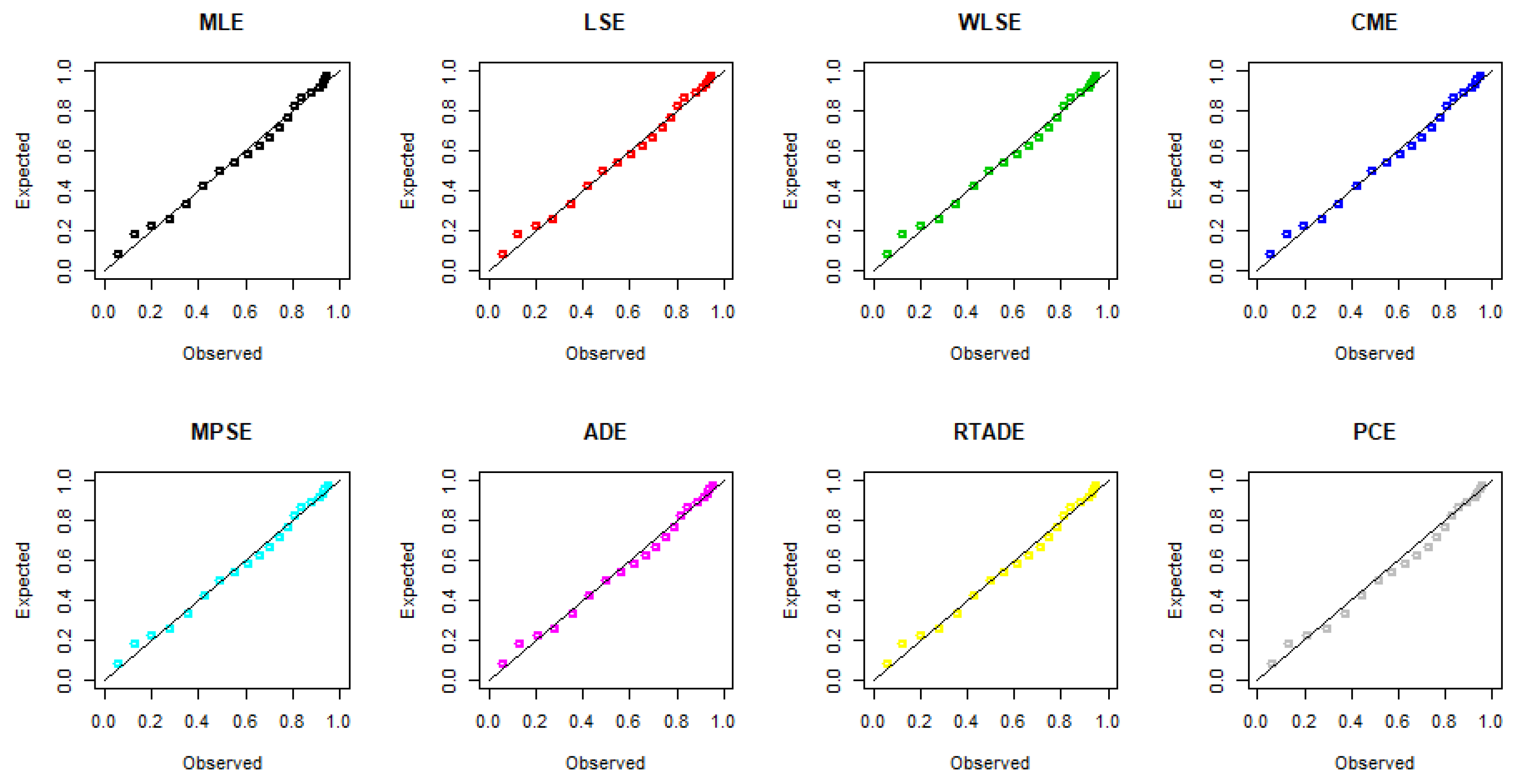
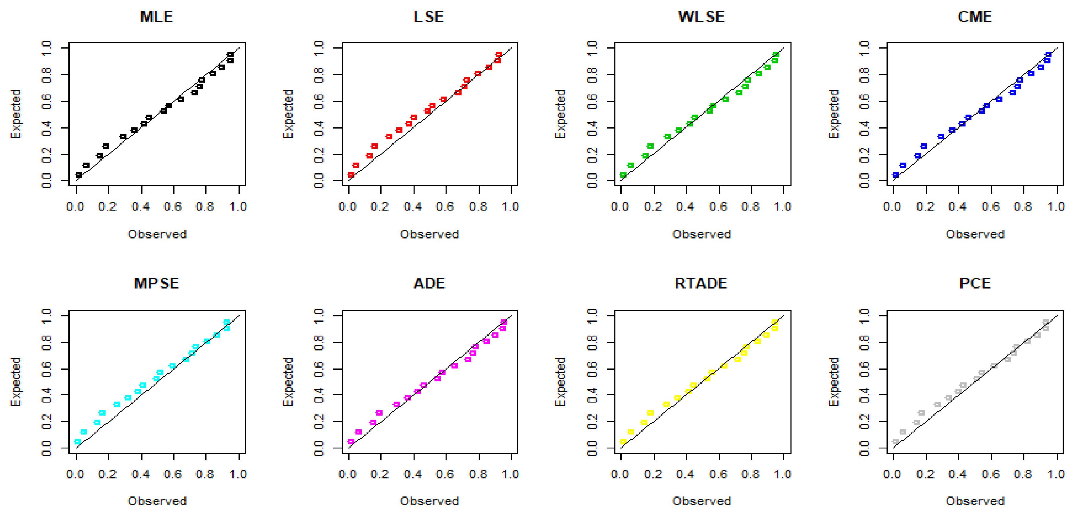
To check the validity of the methods used in this paper to estimate the parameter of the NDL distribution, two different datasets are taken from [9]. One dataset consists of 47 observations representing the daily deaths in Egypt due to COVID-19 infections in the time interval from 8 March to 30 April 2020. The other dataset, measuring remission times in weeks, consists of 20 leukemia patients who were randomly assigned to a certain treatment [25]. Both datasets have been used to illustrate the flexibility of the NDL distribution in modeling similar datasets in estimating the parameter $\theta$. For this purpose, eight methods of estimation have been applied to both datasets.

The estimates of the parameter $\theta$ and goodness-of-fit statistics such as Cramér–von Mises (W), Anderson–Darling (A), and Kolmogorov–Smirnov (KS) statistics, with their associated p-value (KS p-value) are reported in

Table 7. Fitted estimates for COVID-19 and remission times data.

Data	Method	$\widehat{\mathit{\theta }}$	W	A	KS	KS p-Value
Data Set I	MLE	0.18127	0.07635	0.65453	0.09331	0.80785
	LSE	0.18036	0.07640	0.65487	0.09382	0.80248
	WLSE	0.18289	0.07627	0.65393	0.09238	0.81733
	CME	0.18082	0.07637	0.65469	0.09356	0.80522
	MPSE	0.18199	0.076312	0.65426	0.09290	0.81205
	ADE	0.18407	0.07621	0.65349	0.09171	0.82413
	RTADE	0.18381	0.07622	0.65359	0.09186	0.82262
	PCE	0.18915	0.07595	0.65166	0.09413	0.79927
Data Set II	MLE	0.08934	0.01854	0.15568	0.11756	0.94505
	LSE	0.08083	0.01784	0.15275	0.07503	0.99974
	WLSE	0.08923	0.01855	0.15569	0.11792	0.94373
	CME	0.08994	0.01853	0.15560	0.11564	0.95191
	MPSE	0.08201	0.01778	0.15235	0.07120	0.99990
	ADE	0.09058	0.01852	0.15551	0.11355	0.95873
	RTADE	0.08794	0.01857	0.15587	0.12207	0.92686
	PCE	0.08529	0.01864	0.15625	0.13053	0.88506

. Probability–probability (PP) plots for COVID-19 and remission times data for the eight estimates are displayed in Figure 3 and Figure 4, respectively. It is shown, from Table 7 and Figure 3 and Figure 4, that all estimators perform very well.

7. Conclusions and Future Work

The natural discrete Lindley (NDL) distribution has been published as an application of a natural discretization method. However, the published paper did not show its possible applications in significant areas of statistics, like reliability applications. Thus, the main object of this paper has been to widen the usefulness of the NDL distribution through further study of several closure properties under different reliability properties, including the conditions leading to an IFR, as well as hazard rate ordering, reversed hazard rate ordering, and associated results based on these orders.

In addition to the basic results, we also show that the hazard rate ordering of members of the NDL family is preserved under a common contamination. This is quite useful in cases where the systems are operating under random common environments. Important results are derived covering the preservation of the sums of random variables under the hazard rate, likelihood ratio, and reversed hazard rate. Such results are quite useful in the reliability practicing. Furthermore, it is shown that the life lengths of two series systems composed of ordered components of the NDL family preserve the hazard rate order. A basic result gives sufficient conditions for the preservation of the D-MRL property under the assumption of log-concavity of an added contamination. Other, similar results consider the D-MRL case. Finally, an interesting application to renewal processes, which is very helpful in “replacement studies”, is also presented.

The paper is concluded with eight different estimation methods to estimate the parameter $\theta$, and a comparative study has been conducted on their results to explore the behavior of the eight proposed estimators. Two real datasets have been used to explore the behavior of these estimators for estimating the NDL parameter empirically. Each of the methods used has demonstrated acceptable results.

For a possible direction of future studies, the work in this paper can be augmented with the binomial distribution to generate a new model to handle the relationships between the number of particles entering and leaving an attenuator, where several interesting results of value in applications can be established. Compounding results based on adding the life lengths of a random number of components following the NDL distribution could be applied to several insurance problems.