Article

Analytical Estimation of Temperature in Living Tissues Using the TPL Bioheat Model with Experimental Verification

1
Nonlinear Analysis and Applied Mathematics Research Group (NAAM), Department of Mathematics, King Abdulaziz University, Jeddah 21521, Saudi Arabia
2
Department of mathematics, Faculty of Science, Sohag University, Sohag 82524, Egypt
*
Author to whom correspondence should be addressed.
Mathematics 2020, 8(7), 1188; https://doi.org/10.3390/math8071188
Submission received: 5 July 2020 / Revised: 16 July 2020 / Accepted: 17 July 2020 / Published: 19 July 2020
(This article belongs to the Special Issue Modelling and Analysis in Biomathematics)

Abstract

:
The aim of this study is to propose the analytical method associated with Laplace transforms and experimental verification to estimate thermal damages and temperature due to laser irradiation by utilizing measurement information of skin surface. The thermal damages to the tissues are totally estimated by denatured protein ranges using the formulations of Arrhenius. By using Laplace transformations, the exact solution of all physical variables is obtained. Numerical results for the temperature and thermal damage are presented graphically. Furthermore, the comparisons between the numerical calculations with experimental verification show that the three-phase lag bioheat mathematical model is an efficient tool for estimating the bioheat transfer in skin tissue.

1. Introduction

Thermal ablation is a minimally invasive energy-based thermal therapy. It uses extreme temperatures, either high or low, to treat many types of tumors, particularly unresectable tumors, such as liver, kidney, sinus, and lung neoplasms. The heat therapy method has been vastly used in modern medicine, such as in laser tissue soldering [1], laser operations [2], hyperthermia [3], cardiac ablation [4,5,6], laser angioplasty [7,8] and thermal-assisted drug delivery [9,10]. In the field of biomedicine, thermal therapy is used to kill cancerous cells by increasing their temperature to a specific level while avoiding causing damage to the healthy tissues. In thermal therapy, the ultrasound or laser energy passes into the target tissue through triple-layered skin tissue from in vitro to in vivo. It is easy to causes triple-layered skin damage with the heat produced during thermal therapy. Therefore, obtaining the transient temperature field of the triple-layered skin tissue is the key to studying the safety of thermal therapy. Pennes [11] investigated the thermal behavior in forearm skin temperatures, which means that the relation is analyzed by the presented deferment techniques that are used to obtain the solutions of models of heat transfers for infinite thermal propagations, which depend on the Fourier heat conductions. The biological tissue contains many phenomenological mechanizations, such as heating conduction, metabolic heating generation, radiation and the perfusion of blood. In the living tissues, the phase changes occur in wide ranges. Since the variations in temperature in the biological tissues depend on complex phenomena such as blood circulations and metabolic heat generations, authors improved some basic equations. Charny [12] presented the mathematical models of bioheat transfer. Nakayama and Kuwahara [13] studied a general bio-heat transfer model based on the theory of porous media, while Andreozzi et al. [14] presented a modeling heat transfer in tumors: a review of thermal therapies. The dual-phase delay presented by [15] is similar to the modifications of the classical thermoelasticity theory, in which the Fourier law is exchanged by approximations for an improved Fourier law with two differences times: a phase lag of the heat flux, τ q and a phase lag of the temperature gradient, τ θ . According to this theory, the classical law of Fourier, k T = q , has been replaced by
q ( c , t + τ q ) = k T ( c , t + τ θ )
where k is the material thermal conductive, the temperature gradient, T , at a point c of the medium at time t + τ q , corresponds to the vectors of heat flux, q , in time   t + τ q at the same point. This theory is improved rationally to produce a completely consistent theory that is able to commingling heating pulse transmission in very logical ways. Zhu et al. [16] established the sedimentations of lighting energy in tissue and the rate process models for the resulting thermal injuries by using the theorem of diffusions. The bioheat conduction equation upon the dual-phase lag (DPL) was analytically solved, and its results were compared to experimental data, subsequently proving the capability of the proposed DPL model. Additionally, the results of the Fourier model were compared to experimental data, showing that the diffusion model cannot consider microstructural interactions between two phases as well as the local thermal nonequilibrium condition. The generalization is known as the three-phase lag(TPL) thermoelasticity theory, which is given by [17]. According to this theory,
q ( c , t + τ q ) = [ + k * v ( c , t + τ v ) + k T ( c , t + τ θ ) ]
where v ( v ˙ = T ) is the gradient of thermal displacement, τ v is the thermal displacement phase lag for the slope and k * is the material constant characteristic of the model. To study some pertinent and feasible problems, we have found that in heating transfer problems, including very short intervals and in very high heating flux problems, the hyperbolic equation safely provides different outcomes to a greater extent than the parabolic equation. Kumar et al. [18] presented a comparative study of classical Fourier single-phase lag and DPL bio-heat transfer models in tissues. Saeed and Abbas [19] have studied the non-linear DPL bioheat transfer model in a spherical coordinate system. The fractional order bioheat transfer model was studied by Hobiny and Abbas [20]. Mondal et al. [21] studied the effect of the memory-dependent derivatives in the thermal problem in the context of Lord and Shulman (LS) models. Kumar and Chawla [22] studied the three-phase lag for thermoelastic media. Hobiny et al. [23] studied the TPL model of thermo-elastic interactions in the two-dimensional porous mediums due to pulse heat flux. Quintanilla and Racke [24] discussed the stability in the three-phase lag thermal conduction equation and the relationship between the parameters. Abbas and Zenkour [25] studied the effect of dual-phase lag models on the thermo-elastic interaction in semi-infinite media. Abbas and Abbas et al. [26,27,28,29] applied the finite element approach to solve linear and nonlinear thermoelastic problems. Marin [30] studied the Cesaro means in a thermoelastic dipolar body. Marin and Craciun [31] presented the uniqueness result for the boundary value problems in a bipolar thermoelastic model. Hassan et al. [32] investigated the explorations of the convective heating transfer and flow characteristic synthesis.
The aim of this paper is to study the analytical solutions of the temperature and thermal injures of biologicals tissues under TPL models. The numerical outcome can be used as a demonstration division for skin tissues interactions, such as continuous scanning laser interactions. Furthermore, the comparisons among the numerical calculations and the experimental verification indicate that the current three-phase lag bioheat mathematical models is an efficient tool for estimating the bioheat transfer in skin tissue.

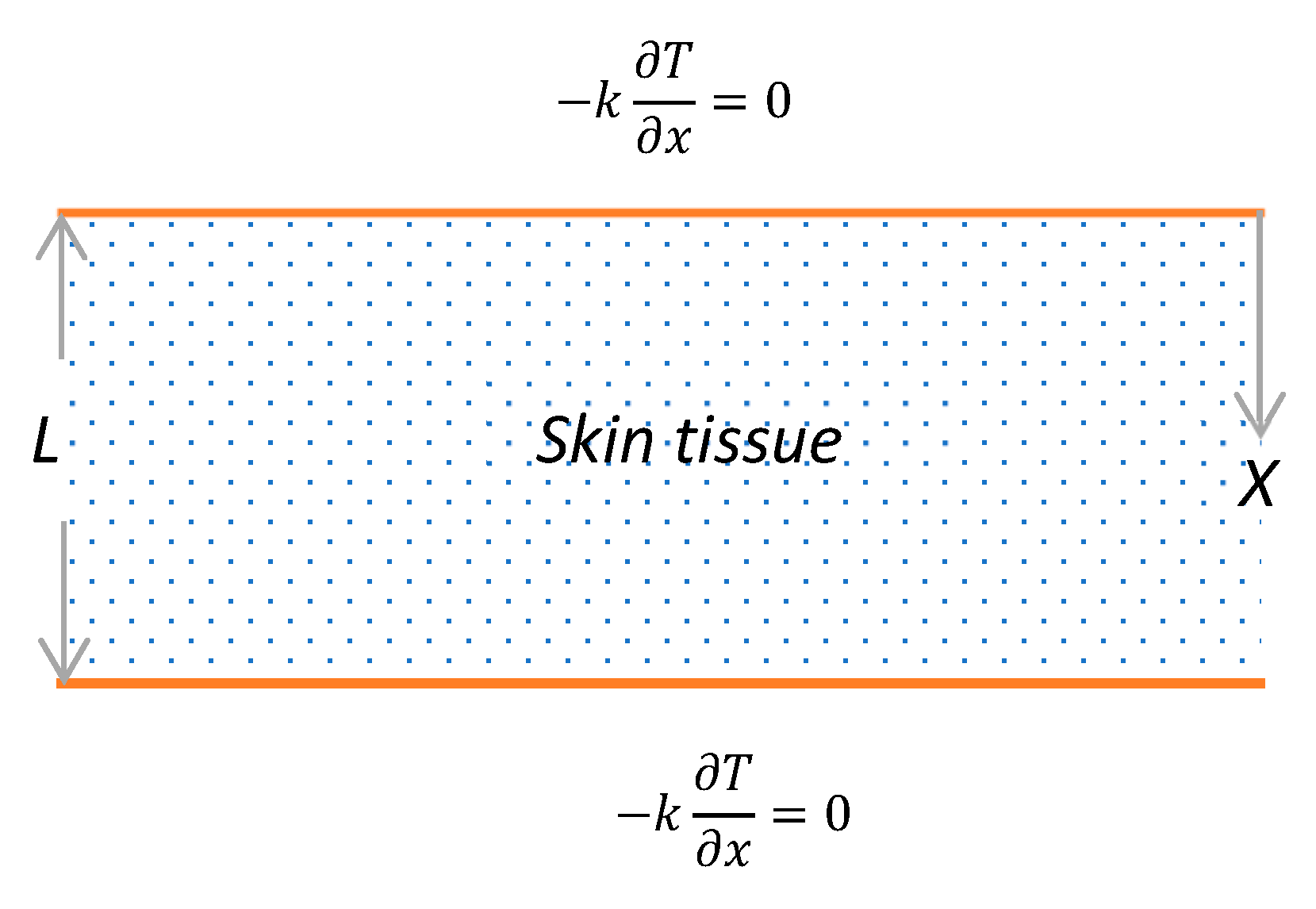
2. Mathematical Model

The problem consists of semi-infinite living tissues that are thermally insulated. The bioheat equation in biological tissues is expressed as [33,34,35]:
[ K * + ( K + K * τ v ) t + K τ θ 2 t 2 ] 2 T x 2 = ( t + τ q 2 t 2 + τ q 2 2 3 t 3 ) ( ρ c T t Q b Q m Q e x t )
where   T is the temperature of tissues; K * is the material constant characteristic of the model; k is the thermal conductivity of tissue; τ θ ,   τ q and τ v denote the delay times, where the delay time   τ q is the phase lag of the heating flux, the phase lag for the gradient of thermal displacement is   τ v and the delay time τ θ is the phase lag of the temperature gradient; t is the time; c is the heating specific of tissue; ρ is the tissues mass density; and   Q b point to the thermal source of blood perfusion which is defined as
Q b = ω b ρ b c b ( T b T )
where   c b is the blood-specific heat, T b is the temperature of blood,   ω b is the rate of blood perfusions, ρ b is the blood mass density, Q m is the heat generated by metabolic processes due to various physiological procedures involved in the rest of the body. Mitchell et al. [36] noted that metabolic thermal productions are functions of local tissue temperatures and can be given as:
Q m = Q m o × 2 β ( T T o 10 )
where T o is the local tissue initial temperature, Q m o is the reference metabolic heating resource and β is the constant-associated metabolic. For all practical objectives, the dependences on metabolic heating generation can be approximated as linear functions of local tissue temperature by the following
Q m = Q m o ( 1 + β ( T T o 10 ) )
where Q e x t is the thermal generated per unit volume of tissue, which is presented by [37] as a laser heating source by:
Q e x t ( x ,   t ) = I o μ a [ U ( t ) U ( t τ p ) ] [ C 1 e k 1 δ x C 2 e k 2 δ x ]
where μ a is the coefficients of absorption; τ p is the exposure time of laser; I o is the laser intensity; δ is penetrations depth; k 1 ,   C 1 ,   k 2 and C 2 are the diffuse reflectance function of R d , which is given in [37]; and U ( t ) is the unit step functions. The penetrations depth was denied by [37]:
δ = 1 3 μ a ( μ a + μ s ( 1 g ) )
where g is the anisotropy factor and μ s is the scattering coefficient. We consider a semi-finite domain of biological tissues with a thickness L , and both of its directions are proposed to be thermally isolated, as in Figure 1 [38]:
Now, initial and boundary conditions can be defined by
T ( x , 0 ) = T b ,   T ( x , 0 ) t = 0
[ K * + ( K + K * τ v ) t + K τ θ 2 t 2 ] T ( L , t ) x = 0 , [ K * + ( K + K * τ v ) t + K τ θ 2 t 2 ] T ( 0 , t ) x = 0
For convenience, the non-dimension variables can be expressed as
T = T T o T o , T b = T b T o T o , ( t , τ θ , τ q , τ v , τ p ) = k ρ c L 2 ( t , τ θ , τ q , τ v , τ p ) , x = x L , f = L 2 K T o , ( k 1 , k 2 ) = L δ ( k 1 , k 2 ) , ( Q b , Q m , Q ext ) = f ( Q b , Q m , Q ext ) , f 1 = f K * .
In terms of these non-dimension forms of variables in (11), the governing Equation (3) with the initial (9) and the boundary (10) conditions is presented by (the dashes are neglected for its appropriateness)
[ f 1 + ( 1 + f 1 τ v ) t + τ θ 2 t 2 ] 2 T x 2 = ( t + τ q 2 t 2 + τ q 2 2 3 t 3 ) ( T t Q b Q m Q e x t )
T ( x , 0 ) = 0 ,   T ( x , 0 ) t = 0
[ f 1 + ( 1 + f 1 τ v ) t + τ θ 2 t 2 ] T ( 0 , t ) x = 0 ,   [ f 1 + ( 1 + f 1 τ v ) t + τ θ 2 t 2 ] T ( L , t ) x = 0

3. Laplace Transforms

The transform of Laplace for any function of M ( x ,   t ) can be given as
M ¯ ( x , s ) = L [ M ( x , t ) ] = 0 M ( x , t ) e s t d t
where s is the parameter of Laplace transforms. Therefore, by using the definitions (15) and the initial conditions (13), the basic Equation (12) and the boundary conditions (15) can be replaced by
d 2 T ¯ d x 2 n 2 T ¯ = n 1 e k 1 x n 2 e k 2 x
T ¯ ( 0 , t ) x = 0 ,   T ¯ ( L , t ) x = 0
where
n 2 = ( s + s 2 τ q + s 3 τ q 2 2 ) ( s + L 2 ω b ρ b c b K L 2 Q m o β 10 K ) f 1 + ( 1 + f 1 τ v ) s + s 2 τ θ ,   n 1 = L 2 I o μ a k T o C 1 ( 1 e s τ p ) f 1 + ( 1 + f 1 τ v ) s + s 2 τ θ   and   n 2 = L 2 I o μ a k T o C 2 ( 1 e s τ p ) f 1 + ( 1 + f 1 τ v ) s + s 2 τ θ .
The general solution T ¯ of the non-homogeneous Equation (16) is the total of two solutions, that is, the particular solution T ¯ p of the non-homogeneous equation with the complementary solution T ¯ c of the associated homogeneous equation. Subsequently, the general solution can be written as
T ¯ ( x , s ) = B 1 e n x + B 2 e n x + n 1 n 2 k 1 2 e k 1 x + n 2 n 2 k 2 2 e k 2 x
To complete the solution, the constants B 1 and B 2 should be determined by using the problem boundary conditions (17) as
B 1 = e Ln ( e Lk 1 ( 1 + e L ( n + k 1 ) ) k 1 n 1 n 2 + k 1 2 + e Lk 2 ( 1 + e L ( n + k 2 ) ) k 2 n 2 n 2 + k 2 2 ) ( 1 + e 2 Ln ) n B 2 = e L ( k 1 + k 2 ) ( e L k 2 ( e L n e L k 1 ) k 1 ( n 2 k 2 2 ) n 1 + e L k 1 ( e L n e L k 2 ) n 2 k 2 n 2 e L k 1 ( e L n e L k 2 ) k 1 2 k 2 n 2 ( 1 + e 2 L n ) n ( n 2 k 1 2 ) ( n 2 k 2 2 )
For final solutions of temperature distributions, a numerically inverse approach adopted which depends on the approximations approach of the Riemann sum is applied to study the numerical calculations. According to this approach, in the Laplace domain, any function can be converted into the time domain as in [39]:
M ( x , t ) = ( R e n = 0 N ( 1 ) n M ¯ ( x , m + i n π t ) + 1 2 R e [ M ¯ ( x , m ) ] ) e m t t
where R e is the actual part and i is the imagery unit number.

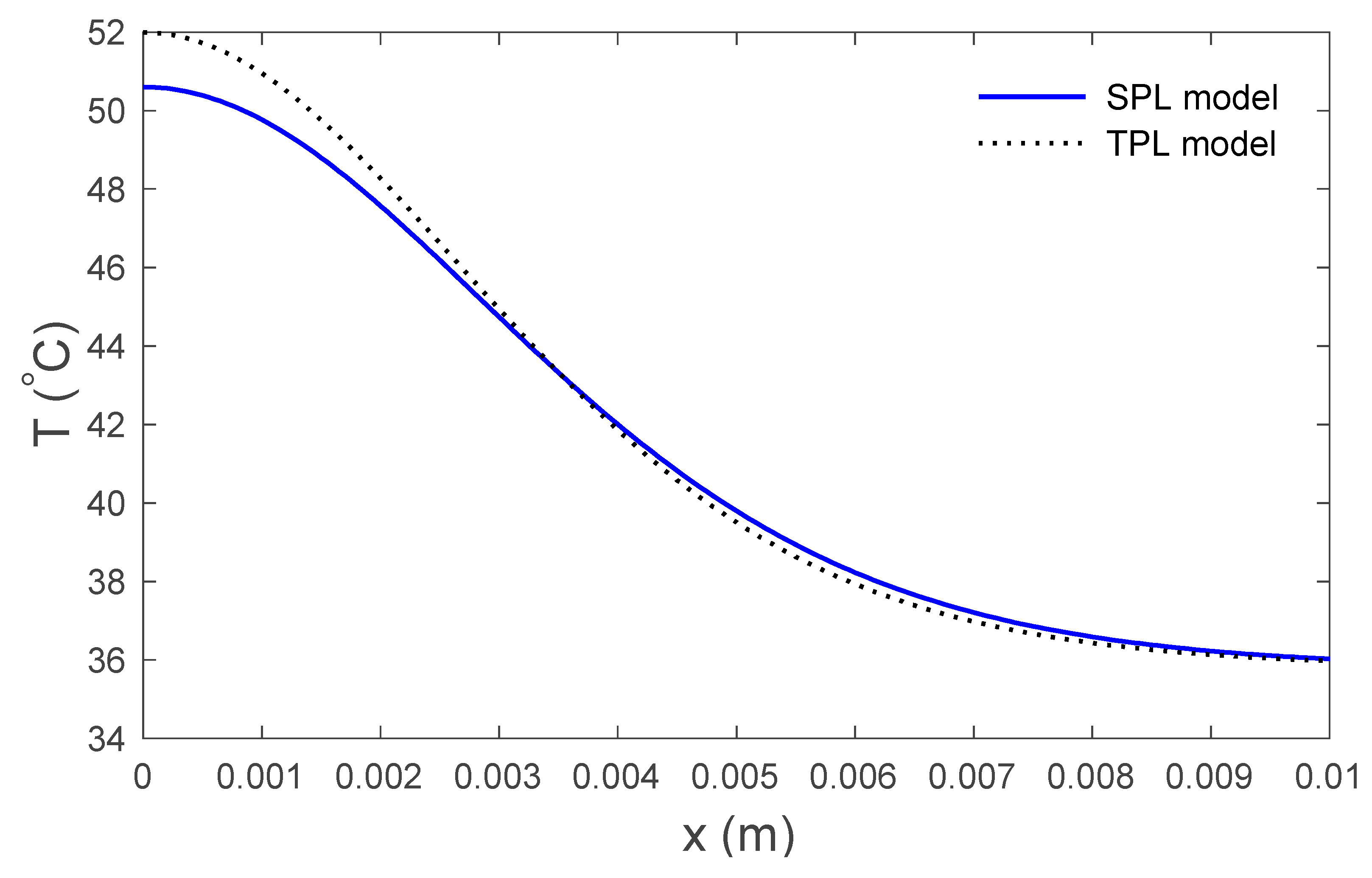
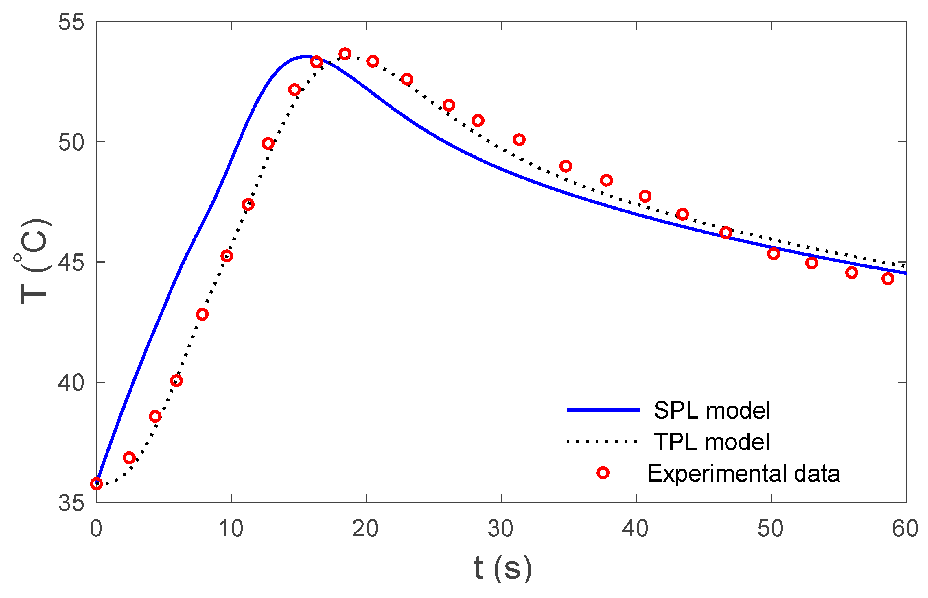
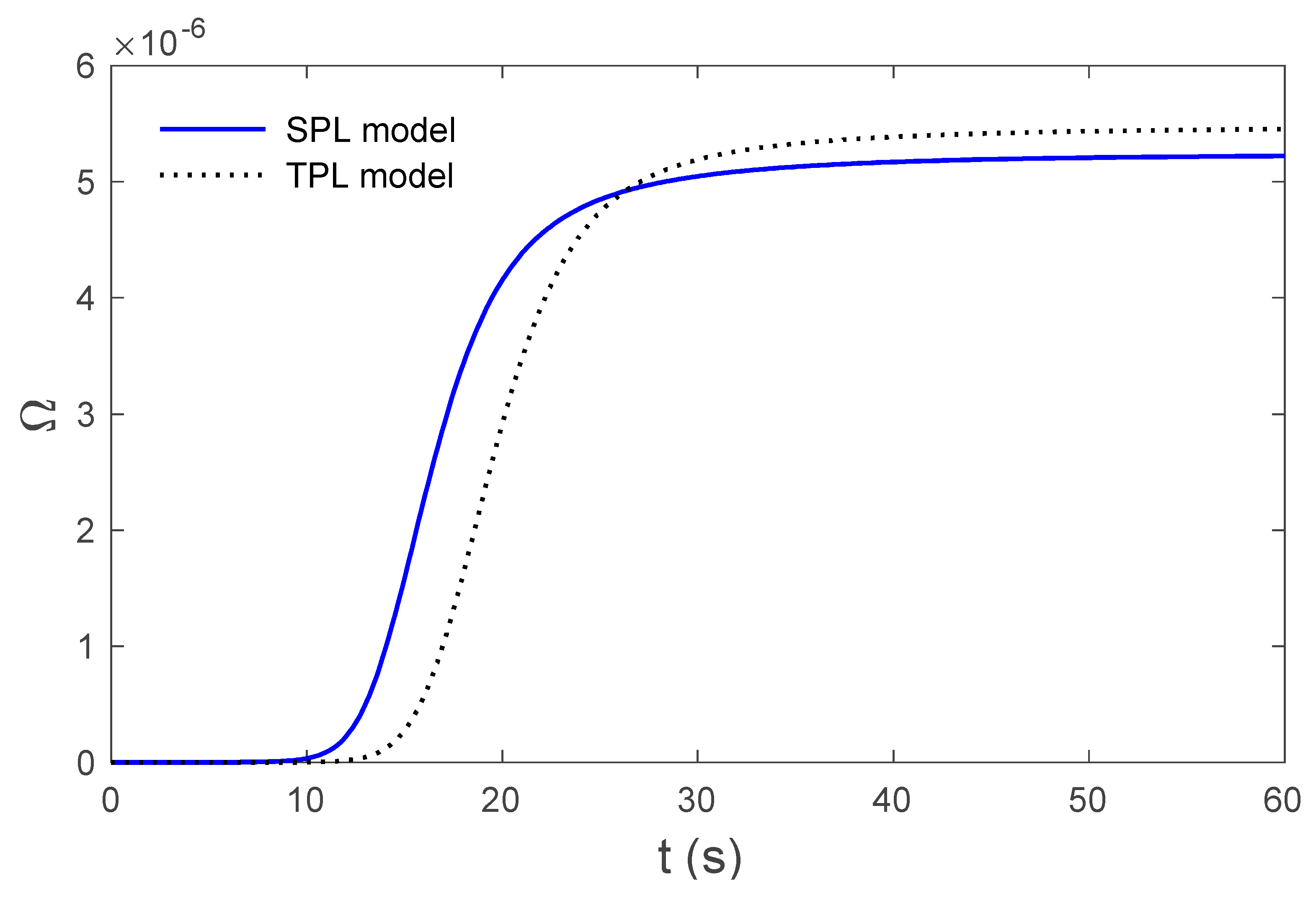
4. Numerical Results and Discussion

For numerical computations, the living tissues were the selections for the purpose of numerical estimation to test the performance of the proposed bio-heat transfer under the three-phase lag model. The values of parameters for biological tissue-like materials are taken as [40]
ρ b = 1060 ( k g ) ( m 3 ) , c b = 3860   ( J ) ( k g 1 ) ( k 1 ) ,   ω b = 1.87 × 10 3 ( s 1 ) ,   T b = 36.5   , I o = 3 × 10 5 ( W ) ( m 2 ) , τ p = 15 ( s ) , L = 0.03 ( m ) ,   Q m = 1.19 × 10 3 ( W ) ( m 3 ) ,   g = 0.9 , C 1 = 3.09 + 5.44 R d 2.12 e 21.5 R d , K 2 = 1.63 e 3.4 R d , C 2 = 2.09 1.47 R d 2.12 e 21.5 R d , K 1 = 1 ( 1 1 3 ) e 20.1 R d , R d = 0.05 , μ s = 12000   ( m 1 ) ,   μ a = 40 ( m 1 ) , T o = 36.5   , ρ = 1000 ( k g ) ( m 3 ) ,   c = 4187   ( J ) ( k g 1 ) ( k 1 ) , k = 0.628   ( W ) ( m 1 ) ( k 1 ) , E a = 6.28 × 10 5   ( J ) ( mol 1 ) ,   R = 8.313   ( J ) ( mol 1 ) ( k 1 ) , B = 3.1 × 10 98 ( s 1 ) .
The accurate prognosis of thermal injuries to living tissues are valuable for thermotherapy. The evaluation of burns is one of the greatest achievements in the area of science that focuses on the bioengineering of biological tissues. To quantify thermal damage, the approach modified by Moritz–Henriques [41,42] was employed. The non-dimension measure of the thermal damage index Ω can expressed as
Ω = 0 t B e E a R T d t ,
where E a is the activation energy, R is the constant of universal gas and B is the frequency factor. Some experimental verifications indicate that there are significant similarities between human and pig skin, especially in the vascular organizations. Museux et al. [43] examine experimental data regarding the heating of pigskin with a laser. There are significant similarities between our analytical solution results and those obtained from the experimental study. Here, the results are based on the skin tissues with the above-mentioned properties, as well as the properties of the blood and the laser parameters. The calculations were made using MATLAB(R2018b) software and the results are graphically presented in Figure 2, Figure 3, Figure 4, Figure 5, Figure 6 and Figure 7. In these figures, the calculation was carried out when T b = T o = 36.5 ° C .
Figure 2 display the variations in temperature versus the distance x for the three-phase lag (TPL) and the single-phase lag (SPL) bioheat transfer models when t = 2   m e n u t e s . It is observed that the temperatures are at their highest at the beginning; they then decrease permanently to T b = 36.6 ° C after x = 9   mm . The variations in surface temperature with time t are displayed in Figure 3. It is clear that the temperature begins from the normal temperature T b and increases with time until the maximum values decrease to the normal temperature. Figure 4 show the variations in thermal damage with respect to the time t . Figure 2, Figure 3 and Figure 4 display the differences between the three-phase lag and the single-phase lag models in the results of thermal damages and the variations in temperature. The solid lines represent the single-phase lag bioheat model, while the dotted lines represent the three-phase lag bioheat model. By comparing the graphs of results obtained under the three-phase lag bioheat model, important phenomena are noted. Figure 5, Figure 6 and Figure 7 show the effects of the blood perfusion rate ω b under the three-phase lag bioheat model on the variations in temperature and thermal damage. The maximum blood perfusions rate, the greatest connective heat loss due to faster blood flows and, subsequently, the smallest magnitude of thermal injury can be seen. From Figure 4 and Figure 7, it observed that initially ( 0 < t < 12   s ) , no such damages occur within the tissues, but with the time-lapse, (i.e., after   t > 12   s) an abrupt increase in damages ( Ω ) is prominently revealed within the tissues.

5. Conclusions

Based on the theory of three-phase lag bio-heat, the variations in temperature and the thermal damage in a living tissue are presented. The non-dimensional outcomes have been solved, employing the semi-analytical approach using the Laplace transforms. The comparisons between the numerical calculations and the existing experimental studies indicate that the three-phase lag mathematical model is an effectives tool to estimate the bio-heat transfer in living tissues.

Author Contributions

All authors conceived the framework and structured the whole manuscript. All authors have read and agreed to the published version of the manuscript.

Funding

This project was founded by the research and development office (RDO) at the ministry of Education, Kingdom of Saudi Arabia. Grant no (HIQI-38-2019). The authors also acknowledge with thanks research and development office (RDO-KAU) at King Abdulaziz University for technical support.

Conflicts of Interest

The authors declare no conflicts of interest.

References

  1. Gabay, I.; Abergel, A.; Vasilyev, T.; Rabi, Y.; Fliss, D.M.; Katzir, A. Temperature-controlled two-wavelength laser soldering of tissues. Lasers Surg. Med. 2011, 43, 907–913. [Google Scholar] [CrossRef] [PubMed]
  2. Zhou, J.; Chen, J.; Zhang, Y. Dual-phase lag effects on thermal damage to biological tissues caused by laser irradiation. Comput. Biol. Med. 2009, 39, 286–293. [Google Scholar] [CrossRef]
  3. Mahjoob, S.; Vafai, K. Analytical characterization of heat transport through biological media incorporating hyperthermia treatment. Int. J. Heat Mass Transf. 2009, 52, 1608–1618. [Google Scholar] [CrossRef]
  4. Labonte, S. Numerical model for radio-frequency ablation of the endocardium and its experimental validation. IEEE Trans. Biomed. Eng. 1994, 41, 108–115. [Google Scholar] [CrossRef] [PubMed]
  5. González-Suárez, A.; Berjano, E. Comparative analysis of different methods of modeling the thermal effect of circulating blood flow during RF cardiac ablation. IEEE Trans. Biomed. Eng. 2015, 63, 250–259. [Google Scholar] [CrossRef] [PubMed] [Green Version]
  6. Iasiello, M.; Andreozzi, A.; Bianco, N.; Vafai, K. The porous media theory applied to radiofrequency catheter ablation. Int. J. Numer. Methods Heat Fluid Flow 2019. [Google Scholar] [CrossRef]
  7. Iasiello, M.; Vafai, K.; Andreozzi, A.; Bianco, N. Hypo-and hyperthermia effects on LDL deposition in a curved artery. Comput. Therm. Sci. Int. J. 2019, 11, 95–103. [Google Scholar] [CrossRef]
  8. Egred, M.; Brilakis, E.S. Excimer laser coronary angioplasty (ELCA): Fundamentals, mechanism of action, and clinical applications. J. Invasive Cardiol. 2020, 32, E27–E35. [Google Scholar]
  9. Ho, Y.-J.; Wu, C.-C.; Hsieh, Z.-H.; Fan, C.-H.; Yeh, C.-K. Thermal-sensitive acoustic droplets for dual-mode ultrasound imaging and drug delivery. J. Control. Release 2018, 291, 26–36. [Google Scholar] [CrossRef]
  10. Andreozzi, A.; Iasiello, M.; Netti, P.A. A thermoporoelastic model for fluid transport in tumour tissues. J. R. Soc. Interface 2019, 16, 20190030. [Google Scholar] [CrossRef] [Green Version]
  11. Pennes, H.H. Analysis of tissue and arterial blood temperatures in the resting human forearm. J. Appl. Physiol. 1948, 1, 93–122. [Google Scholar] [CrossRef]
  12. Charny, C.K. Mathematical models of bioheat transfer. In Advances in Heat Transfer; Elsevier: Amsterdam, The Netherlands, 1992; Volume 22, pp. 19–155. [Google Scholar]
  13. Nakayama, A.; Kuwahara, F. A general bioheat transfer model based on the theory of porous media. Int. J. Heat Mass Transf. 2008, 51, 3190–3199. [Google Scholar] [CrossRef] [Green Version]
  14. Andreozzi, A.; Brunese, L.; Iasiello, M.; Tucci, C.; Vanoli, G.P. Modeling heat transfer in tumors: A review of thermal therapies. Ann. Biomed. Eng. 2019, 47, 676–693. [Google Scholar] [CrossRef] [PubMed]
  15. Tzou, D.Y. A Unified field approach for heat conduction from macro- to micro-scales. J. Heat Transf. 1995, 117, 8–16. [Google Scholar] [CrossRef]
  16. Zhu, D.; Luo, Q.; Zhu, G.; Liu, W. Kinetic thermal response and damage in laser coagulation of tissue. Lasers Surg. Med. 2002, 31, 313–321. [Google Scholar] [CrossRef] [PubMed]
  17. Choudhuri, S.R. On a thermoelastic three-phase-lag model. J. Therm. Stresses 2007, 30, 231–238. [Google Scholar] [CrossRef]
  18. Kumar, D.; Singh, S.; Rai, K. Analysis of classical Fourier, SPL and DPL heat transfer model in biological tissues in presence of metabolic and external heat source. Heat Mass Transf. 2016, 52, 1089–1107. [Google Scholar] [CrossRef]
  19. Saeed, T.; Abbas, I. Finite element analyses of nonlinear DPL bioheat model in spherical tissues using experimental data. Mech. Based Des. Struct. Mach. 2020, 1–11. [Google Scholar] [CrossRef]
  20. Hobiny, A.; Abbas, I. Analytical solutions of fractional bioheat model in a spherical tissue. Mech. Based Des. Struct. Mach. 2019, 1–10. [Google Scholar] [CrossRef]
  21. Mondal, S.; Sur, A.; Kanoria, M. Transient heating within skin tissue due to time-dependent thermal therapy in the context of memory dependent heat transport law. Mech. Based Des. Struct. Mach. 2019, 1–15. [Google Scholar] [CrossRef]
  22. Kumar, R.; Chawla, V. Reflection and refraction of plane wave at the interface between elastic and thermoelastic media with three-phase-lag model. Int. Commun. Heat Mass Transf. 2013, 48, 53–60. [Google Scholar] [CrossRef]
  23. Hobiny, A.; Alzahrani, F.S.; Abbas, I. Three-phase lag model of thermo-elastic interaction in a 2D porous material due to pulse heat flux. Int. J. Numer. Methods Heat Fluid Flow 2020. [Google Scholar] [CrossRef]
  24. Quintanilla, R.; Racke, R. A note on stability in three-phase-lag heat conduction. Int. J. Heat Mass Transf. 2008, 51, 24–29. [Google Scholar] [CrossRef] [Green Version]
  25. Abbas, I.A.; Zenkour, A.M. Dual-phase-lag model on thermoelastic interactions in a semi-infinite medium subjected to a ramp-type heating. J. Comput. Theor. Nanosci. 2014, 11, 642–645. [Google Scholar] [CrossRef]
  26. Abbas, I.A.; Youssef, H.M. Two-temperature generalized thermoelasticity under ramp-type heating by finite element method. Meccanica 2013, 48, 331–339. [Google Scholar] [CrossRef]
  27. Abbas, I.A. Finite element analysis of the thermoelastic interactions in an unbounded body with a cavity. Forschung im Ingenieurwesen 2007, 71, 215–222. [Google Scholar] [CrossRef]
  28. Abbas, I.A.; Abo-El-Nour, N.; Othman, M.I. Generalized magneto-thermoelasticity in a fiber-reinforced anisotropic half-space. Int. J. Thermophys. 2011, 32, 1071–1085. [Google Scholar] [CrossRef]
  29. Zenkour, A.M.; Abbas, I.A. A generalized thermoelasticity problem of an annular cylinder with temperature-dependent density and material properties. Int. J. Mech. Sci. 2014, 84, 54–60. [Google Scholar] [CrossRef]
  30. Marin, M. Cesaro means in thermoelasticity of dipolar bodies. Acta Mech. 1997, 122, 155–168. [Google Scholar] [CrossRef]
  31. Marin, M.; Craciun, E. Uniqueness results for a boundary value problem in dipolar thermoelasticity to model composite materials. Compos. Part B Eng. 2017, 126, 27–37. [Google Scholar] [CrossRef]
  32. Hassan, M.; Marin, M.; Ellahi, R.; Alamri, S.Z. Exploration of convective heat transfer and flow characteristics synthesis by Cu–Ag/water hybrid-nanofluids. Heat Transf. Res. 2018, 49, 1837–1848. [Google Scholar] [CrossRef]
  33. Xu, F.; Seffen, K.; Lu, T. Non-Fourier analysis of skin biothermomechanics. Int. J. Heat Mass Transf. 2008, 51, 2237–2259. [Google Scholar] [CrossRef]
  34. Ahmadikia, H.; Fazlali, R.; Moradi, A. Analytical solution of the parabolic and hyperbolic heat transfer equations with constant and transient heat flux conditions on skin tissue. Int. Commun. Heat Mass Transf. 2012, 39, 121–130. [Google Scholar] [CrossRef]
  35. Kumar, D.; Rai, K. Three-phase-lag bioheat transfer model and its validation with experimental data. Mech. Based Des. Struct. Mach. 2020, 1–15. [Google Scholar] [CrossRef]
  36. Mitchell, J.W.; Galvez, T.L.; Hengle, J.; Myers, G.E.; Siebecker, K.L. Thermal response of human legs during cooling. J. Appl. Physiol. 1970, 29, 859–865. [Google Scholar] [CrossRef]
  37. Gardner, C.M.; Jacques, S.L.; Welch, A. Light transport in tissue: Accurate expressions for one-dimensional fluence rate and escape function based upon Monte Carlo simulation. Lasers Surg. Med. Off. J. Am. Soc. Laser Med. Surg. 1996, 18, 129–138. [Google Scholar] [CrossRef]
  38. Hobiny, A.D.; Abbas, I.A. Theoretical analysis of thermal damages in skin tissue induced by intense moving heat source. Int. J. Heat Mass Transf. 2018, 124, 1011–1014. [Google Scholar] [CrossRef]
  39. Tzou, D.Y. Macro-to Micro-Scale Heat Transfer: The Lagging Behavior; CRC Press: Boca Raton, FL, USA, 1996. [Google Scholar]
  40. Noroozi, M.J.; Goodarzi, M. Nonlinear analysis of a non-Fourier heat conduction problem in a living tissue heated by laser source. Int. J. Biomath. 2017, 10, 1750107. [Google Scholar] [CrossRef]
  41. Henriques, F., Jr.; Moritz, A. Studies of thermal injury: I. The conduction of heat to and through skin and the temperatures attained therein. A theoretical and an experimental investigation. Am. J. Pathol. 1947, 23, 530. [Google Scholar]
  42. Moritz, A.R.; Henriques, F., Jr. Studies of thermal injury: II. The relative importance of time and surface temperature in the causation of cutaneous burns. Am. J. Pathol. 1947, 23, 695–720. [Google Scholar]
  43. Museux, N.; Perez, L.; Autrique, L.; Agay, D. Skin burns after laser exposure: Histological analysis and predictive simulation. Burns 2012, 38, 658–667. [Google Scholar] [CrossRef] [PubMed] [Green Version]
Figure 1. One-dimensional schematic geometry of skin.
Mathematics 08 01188 g001
Figure 2. Variations in temperature versus the distance for the SPL and the TPL models.
Mathematics 08 01188 g002
Figure 3. Temperature at the skin surface for the SPL and TPL models in relation to time.
Mathematics 08 01188 g003
Figure 4. Variations in thermal damage for the SPL and TPL models at the skin surface x = 0 .
Mathematics 08 01188 g004
Figure 5. Variations in temperature versus the distance under the TPL model for several values of the rate of blood perfusion ω b .
Mathematics 08 01188 g005
Figure 6. Temperature under the TPL model for several values of the rate of blood perfusion ω b at the skin surface in relation to time.
Mathematics 08 01188 g006
Figure 7. Variations in thermal damage under the TPL model for several values of the rate of blood perfusion ω b at the skin surface x = 0 .
Mathematics 08 01188 g007

