A Multi-Criteria Decision-Making Method Based on Single-Valued Neutrosophic Partitioned Heronian Mean Operator

Abstract

A multi-criteria decision-making (MCDM) method with single-valued neutrosophic information is developed based on the Partitioned Heronian Mean (PHM) operator and the Shapley fuzzy measure, which recognizes correlation among the selection criteria. Motivated by the PHM operator and Shapley fuzzy measure, two new aggregation operators, namely the single-valued neutrosophic PHM operator and the weighted single-valued neutrosophic Shapley PHM operator, are defined, and their corresponding properties and some special cases are investigated. An MCDM model is applied to solve the single-valued neutrosophic problem where weight information is not completely known. An example is provided to validate the proposed method.

1. Introduction

Zadeh first put forward the notion of fuzzy sets (FSs) [1]. Since then, multi-criteria decision-making (MCDM) methods based on FSs have been well developed and applied to hotel selection [2], investment project selection [3], supplier selection [4], solar power station site selection [5], recycling waste resource evaluation [6], and others [7,8,9,10,11,12,13]. However, due to the inherent subjectivity in the preferences of the decision makers (DMs), a single membership degree of FSs cannot adequately capture the subjectivity and uncertainty in the decision-making process. In view of this, Atanassov [14] introduced intuitionistic fuzzy sets (IFSs), including membership and non-membership degrees and a hesitation index, as an extension of FSs. However, both FSs and IFSs are not adept at tackling problems involving information uncertainty. For example, when we ask an expert about a certain statement, the expert may say the probability that the statement is true, false, and unsure is 0.6, 0.5, and 0.1 respectively [15]. Clearly, the solution to this problem is beyond the scope of FSs and IFSs. Smarandache et al. [16] constructed neutrosophic sets (NSs) that involve three membership functions: truth, indeterminacy, and falsity. It is noted that NSs lie on a non-standard unit interval ]0⁻, 1⁺[ [17], which is an extension of the standard interval [0.1] of IFSs. The uncertainty presented here, i.e., the indeterminacy factor, depends on the truth and falsity values while the incorporated uncertainty depends on the membership and non-membership degrees of the IFSs [18]. Thus, the earlier example of NSs can be expressed as x(0.6, 0.1, 0.5). While some MCDM methods with neutrosophic information have been investigated [19,20,21], their applicability is restricted because of the non-standard unit interval. As such, single-valued neutrosophic sets (SVNSs) were proposed, as a special case of NSs [22].

SVNSs have recently become a popular method to describe the preference information of DMs, and have attracted much research attention in areas such as aggregation operators [23,24,25,26,27,28], outranking relations [29], and information measures [30,31,32,33].

Indeed, aggregation operators are significant in solving MCDM problems. Different functions usually involve different aggregation operators such as the Heronian mean (HM) operator [34,35], Hamacher operator [36,37], Muirhead mean operator [38,39], Maclaurin symmetric mean operator [40,41], and Bonferroni mean operator [42,43,44]. These operators can reduce the effects of abnormal data provided by DMs. For instance, the HM operator, defined by Sykora [34], takes the interrelationship of the input arguments into account. Recently, many studies have examined the HM operator and extended it to various decision-making contexts. For instance, based on the HM operator, Liu and Shi [35] defined some neutrosophic linguistic operators and Peng et al. [45] discussed the single-valued neutrosophic hesitant fuzzy geometric Choquet integral HM operator. In addition, some other MCDM methods, including the analytic network process (ANP) [46], and the analytic hierarchy process and interpretive structural modelling (AHP-ISM) [47,48], also consider the interrelationship of criteria. However, the HM operator, ANP, and AHP-ISM presuppose that all the selection criteria are interrelated. In reality, the criteria need not always be correlated with each other. Hence, the criteria should be partitioned into distinct categories to improve decision-making accuracy. Liu et al. [49] defined the partitioned HM (PHM) operator where all the criteria are partitioned into categories, in which the criteria in the same category are correlated with each other. For example, if a firm wishes to select a food supplier from several vendors using the criteria of cost (c₁), quality (c₂), service performance (c₃), risk (c₄), and supplier profile (c₅), then the criteria can be partitioned into the categories P₁ = {c₁, c₂, c₄} and P₂ = {c₃, c₅}. Criteria c₁, c₂ and c₄ are correlated, placing them in the same category, P₁; likewise, for criteria c₃ and c₅ in set P₂. It is noted that the Shapley fuzzy measure [50,51] is adept at handling MCDM problems with correlated selection criteria, and has been extensively used for the same reason [52,53].

From the analysis presented above, the motivations of this research can be concluded as: (1) the existing single-valued neutrosophic aggregation operators only consider the importance of assessment values or that of the ordered position, but ignore the complex interrelationship of the criteria; (2) the existing methods are mostly constructed under complete weight information, and cannot deal with MCDM problems where the weight information is incomplete. Thus, our study makes two contributions. First, we propose two new partitioned aggregation operators, namely, the single-valued neutrosophic PHM (SVNPHM) operator and the weighted single-valued neutrosophic Shapley PHM (WSVNSPHM) operator, to avoid the first shortcoming. Next, we develop a method to deal with the single-valued neutrosophic MCDM problem under incomplete weight information, to handle the second shortcoming.

The rest of this paper is set as follows. In Section 2, some definitions are introduced. The SVNPHM and WSVNSPHM operators are explained in Section 3. The single-valued MCDM method with incomplete weight information is developed in Section 4. In Section 5, an example is provided to validate the proposed method. Finally, conclusions are drawn in Section 6.

2. Preliminaries

Here, we introduce some definitions, namely, the Shapley fuzzy measure, PHM operator, NSs, and SVNSs.

2.1. Shapley Fuzzy Measure

Definition 1

[50]. Let $X=\left\{x_1,x_2,\dots ,x_n\right\}$ be a space of objects and $P\left(x\right)$ be the power set of $X$. Then the function $\mu :\left(P\left(x\right)\to \left[0,1\right]\right)$ is defined as a fuzzy measure, satisfying

(1)

$\mu \left(\mathsf{\Phi }\right)=0$and$\mu \left(X\right)=1$;

(2)

$\forall \alpha ,\beta \in P\left(X\right)$and$\alpha \subseteq \beta$, then$\mu \left(\alpha \right)\le \mu \left(\beta \right)$.

Definition 2

([54]). Suppose $\mu$ is a fuzzy measure on $X$. The corresponding Möbius transformation can be expressed as

$$\beta \subset X,m\left(\beta \right)={\displaystyle \sum _{\alpha \subset \beta }{\left(-1\right)}^{\left|\beta \backslash \alpha \right|}}\mu \left(\alpha \right)$$

(1)

If$\left|\beta \right|=k,m\left(\beta \right)=0$and there exists at least one subset$\gamma \left(\left|\gamma \right|=k\right)$satisfying$m\left(\gamma \right)\ne 0$, then$\mu$is called a k-order additive fuzzy measure.

Definition 3

([50]). Suppose μ is a fuzzy measure on X; the Shapley value to measure the average importance degree of S is:

$${\tau }_S\left(\mu ,X\right)={\displaystyle \sum _{M\subseteq X\backslash S}\frac{\left(n-s-m\right)!m!}{\left(n-s+1\right)!}\left(\mu \left(S\cup \left\{M\right\}\right)-\mu \left(M\right)\right)},\forall S\subseteq X$$

(2)

where n, m, and s denote the cardinalities of $X$, $M$, and $S$, respectively. As noted in [54], ${\tau }_S\left(\mu ,X\right)\ge 0$ and ${\displaystyle \sum _{S\subseteq X}{\tau }_S\left(\mu ,X\right)}=1$. ${\tau }_S\left(\mu ,X\right)$ is called Shapley fuzzy measures [53].

In this paper, the Shapley fuzzy measures are additive fuzzy measures unless otherwise stated.

Example 1.

Suppose$X=\left\{d,e,f\right\}$, and$\mu$is a fuzzy measure, with$\mu (\varnothing )=0$,$\mu \left(\left\{d\right\}\right)=0.1$,$\mu \left(\left\{e\right\}\right)=0.2$,$\mu \left(\left\{f\right\}\right)=0.5$,$\mu \left(\left\{d,e\right\}\right)=0.5$,$\mu \left(\left\{e,f\right\}\right)=0.9$,$\mu \left(\left\{d,f\right\}\right)=0.8$, and$\mu \left(\left\{X\right\}\right)=1$. If$S=\left\{d,e\right\}$, then$X\backslash S=\left\{f\right\}$. The following results can be obtained:

$$\begin{array}{cc}\hfill {\varphi }_S\left(\mu ,X\right)=& \frac{\left(3-2-1\right)!1!}{\left(3-2+1\right)!}\left(\mu \left(\left\{d,e\right\}\cup \left\{f\right\}\right)-\mu \left(\left\{f\right\}\right)\right)+\frac{\left(3-2-0\right)!0!}{\left(3-2+1\right)!}\left(\mu \left(\left\{d,e\right\}\cup \{\varnothing \}\right)-\mu \left(\left\{f\right\}\right)\right)\hfill \\ \hfill =& \frac{1}{2}\left(\mu \left(d,e,f\right)-\mu \left(f\right)\right)+\frac{1}{2}\left(\mu \left(d,e\right)-\mu (\varnothing )\right)\hfill \\ \hfill =& \frac{1}{2}\left(1-0.5\right)+\frac{1}{2}\left(0.5-0\right)=0.5.\hfill \end{array}$$

2.2. PHM

Definition 4

([34]). Let ${\chi }_i\left(i=1,2,\dots ,n\right)$ be a set of real numbers. The HM operator is defined as:

$$H{M}_{p,q}\left({\chi }_1,{\chi }_2,\dots ,{\chi }_n\right)={\left(\frac{2}{n\left(n+1\right)}{\displaystyle \sum _{i=1,j=i}^n{\chi }_i{}^p{\chi }_j{}^q}\right)}^{\frac{1}{p+q}}$$

(3)

where $p,q\ge 0$, and the HM operator satisfies the following properties:

(1)

Idempotency: If${\chi }_i=\chi \left(i=1,2,\dots ,n\right)$, then$H{M}_{p,q}\left(\chi ,\chi ,\dots ,\chi \right)=\chi$.

(2)

Permutability: If${\chi }_i{}^{\prime }\left(i=1,2,\dots ,n\right)$is a permutation of${\chi }_i\left(i=1,2,\dots ,n\right)$, then$H{M}_{p,q}\left({\chi }_1{}^{\prime },{\chi }_2{}^{\prime },\dots ,{\chi }_n{}^{\prime }\right)=H{M}_{p,q}\left({\chi }_1,{\chi }_2,\dots ,{\chi }_n\right)$.

(3)

Boundedness: If${\chi }^{+}=\max \left\{{\chi }_1,{\chi }_2,\dots ,{\chi }_n\right\}$and${\chi }^{-}=\min \left\{{\chi }_1,{\chi }_2,\dots ,{\chi }_n\right\}$, then${\chi }^{-}\le H{M}_{p,q}\left({\chi }_1,{\chi }_2,\dots ,{\chi }_n\right)\le {\chi }^{+}$.

Definition 5

([49]). Let ${\chi }_i\left(i=1,2,\dots ,n\right)$ be a set of inputs that can be partitioned into $t$ categories $P_l\left(l=1,2,\dots ,t\right)$. The PHM operator is defined as:

$$PH{M}_{p,q}\left({\chi }_1,{\chi }_2,\dots ,{\chi }_n\right)=\frac{1}{t}\left({\displaystyle \sum _{l=1}^t{\left(\frac{2}{\left|P_l\right|\left(\left|P_l\right|+1\right)}{\displaystyle \sum _{i=1,j=i}^{\left|P_l\right|}{\chi }_i^p{\chi }_j^q}\right)}^{\frac{1}{p+q}}}\right)$$

(4)

where $p,q\ge 0$, $p+q>0$, ${\displaystyle \sum _{l=1}^t\left|P_l\right|}=n$, and $P_i\cap P_j=\varnothing$, and $\left|P_l\right|$ denotes the cardinality of $P_l$.

Example 2.

If$C=\left\{c_1,c_2,c_3,c_4,c_5\right\}$is a set of criteria that can be partitioned into two categories P₁ = {c₁, c₂, c₃} and P₂ = {c₄, c₅}, and the assessment values provided by the DMs are$\chi =\left\{0.7,0.5,0.4,0.6,0.8\right\}$(for convenience, let p = q = 1), then, the aggregated results using the PHM operator are written as:

$$\begin{array}{l}PH{M}_{1,1}\left({\chi }_1,{\chi }_2,\dots ,{\chi }_5\right)=\frac{1}{2}\left({\left(\frac{2}{\left|P_1\right|\left(\left|P_1\right|+1\right)}{\displaystyle \sum _{i=1,j=i}^{\left|P_1\right|}{\chi }_i^1{\chi }_j^1}\right)}^{\frac{1}{2}}+{\left(\frac{2}{\left|P_2\right|\left(\left|P_2\right|+1\right)}{\displaystyle \sum _{i=4,j=i}^{\left|P_2\right|}{\chi }_i^1{\chi }_j^1}\right)}^{\frac{1}{2}}\right)\\ =\frac{1}{2}({\left(\frac{2}{3\times 4}\left(0.7\times 0.7+0.7\times 0.5+0.7\times 0.4+0.5\times 0.5+0.5\times 0.4+0.4\times 0.4\right)\right)}^{\frac{1}{2}}+\\ {\left(\frac{2}{2\times 3}\left(0.6\times 0.6+0.6\times 0.8+0.8\times 0.8\right)\right)}^{\frac{1}{2}})=\frac{1}{2}\left(0.5369+0.7024\right)=0.6197.\end{array}$$

Moreover,

$$\begin{array}{l}H{M}_{1,1}\left({\chi }_1,{\chi }_2,\dots ,{\chi }_5\right)={\left(\frac{2}{5\times 6}{\displaystyle \sum _{i=1,j=i}^m{\chi }_i{}^1{\chi }_j{}^1}\right)}^{\frac{1}{2}}\\ \begin{array}{cc}\hfill =\frac{2}{5\times 6}& (0.7\times 0.7+0.7\times 0.5+0.7\times 0.4+0.7\times 0.6+0.7\times 0.8+0.5\times 0.5+0.5\times 0.4+0.5\times 0.6\hfill \\ \hfill +& 0.5\times 0.8+0.4\times 0.4+0.4\times 0.6+0.4\times 0.8+0.6\times 0.6+0.6\times 0.8+0.8\times 0.8)\hfill \end{array}\\ ={\left(\frac{4.81}{15}\right)}^{\frac{1}{2}}=0.5663.\end{array}$$

The reason for the difference in the results obtained by the PHM operator and those obtained by the HM operator is that the PHM operator partitions the input values into categories based on the relationship of the values, whereas the HM operator presupposes the condition that each input value is correlated with the other values. Therefore, the PHM operator is more reasonable than the HM operator.

2.3. NSs and SVNSs

Definition 6

[16]. An NS $\tilde{S}$ in $X=\left\{x_1,x_2,\dots ,x_n\right\}$ can be characterized as $\tilde{S}=\left\{\langle x,{\tilde{T}}_{\tilde{S}}(x),{\tilde{I}}_{\tilde{S}}(x),{\tilde{F}}_{\tilde{S}}(x)\rangle |x\in X\right\}$, where ${\tilde{T}}_{\tilde{S}}\left(x\right)$, ${\tilde{I}}_{\tilde{S}}\left(x\right)$, and ${\tilde{F}}_{\tilde{S}}\left(x\right)$ denote the truth, indeterminacy, and falsity memberships respectively. Furthermore, ${\tilde{T}}_{\tilde{S}}\left(x\right)$, ${\tilde{I}}_{\tilde{S}}\left(x\right)$, and ${\tilde{F}}_{\tilde{S}}\left(x\right)$ are subsets of $]0^{-},1^{+}[$, that is, ${\tilde{T}}_{\tilde{S}}\left(x\right):X\to ]0^{-},1^{+}[$, ${\tilde{I}}_{\tilde{S}}\left(x\right):X\to ]0^{-},1^{+}[$, and ${\tilde{F}}_{\tilde{S}}\left(x\right):X\to ]0^{-},1^{+}[$satisfy the condition $0^{-}\le \sup {\tilde{T}}_{\tilde{S}}\left(x\right)+\sup {\tilde{I}}_{\tilde{S}}\left(x\right)+\sup {\tilde{F}}_{\tilde{S}}\left(x\right)\le 3^{+}$.

Since it is impractical for NSs to tackle real-life problems because of their nonstandard intervals, Majumdar and Samant [18] defined SVNSs based on standard intervals, and Ye [19] developed the corresponding properties for SVNSs.

Definition 7

([22]). An SVNS $S$ in $X=\left\{x_1,x_2,\dots ,x_n\right\}$ is defined as $S=\left\{\langle x,T_S\left(x\right),I_S\left(x\right),F_S\left(x\right)\rangle |x\in X\right\}$, where $T_S\left(x\right)$, $I_S\left(x\right)$, and $F_S\left(x\right)$ are subsets in the standard interval [0, 1], i.e., $T_S\left(x\right):X\to [0,1]$, $I_S\left(x\right):X\to [0,1]$, and $F_S\left(x\right):X\to [0,1]$. If $\mathrm{X}$ has only one element, then $S$ is a single-valued neutrosophic number (SVNN). For convenience, we denote the SVNN by $S=\langle T_S,I_S,F_S\rangle$.

Definition 8

([22]). Let $S=\langle T_S,I_S,F_S\rangle$, $S_1=\langle T_{S_1},I_{S_1},F_{S_1}\rangle$, and $S_2=\langle T_{S_2},I_{S_2},F_{S_2}\rangle$ be three SVNNs. With $\lambda >0$, the following properties hold:

(1)

$\lambda S=\langle 1-{\left(1-T_S\right)}^{\lambda },1-{\left(1-I_S\right)}^{\lambda },1-{\left(1-F_S\right)}^{\lambda }\rangle ,\lambda >0$;

(2)

$S^{\lambda }=\langle T_S^{\lambda },I_S^{\lambda },F_S^{\lambda }\rangle ,\lambda >0$;

(3)

$S_1\oplus S_2=\langle T_{S_1}+T_{S_2}-T_{S_1}\cdot T_{S_2},I_{S_1}+I_{S_2}-I_{S_1}\cdot I_{S_2},F_{S_1}+F_{S_2}-F_{S_1}\cdot F_{S_2}\rangle$;

(4)

$S_1\otimes S_2=\langle T_{S_1}\cdot T_{S_2},I_{S_1}\cdot I_{S_2},F_{S_1}\cdot F_{S_2}\rangle$.

However, as stated in [19], the above operations are unreasonable. In view of this, Peng et al. [20] improved the properties of SVNNs as well as the corresponding comparison method.

Definition 9

([23]). Let $S=\langle T_S,I_S,F_S\rangle$, $S_1=\langle T_{S_1},I_{S_1},F_{S_1}\rangle$, and $S_2=\langle T_{S_2},I_{S_2},F_{S_2}\rangle$ be three SVNNs. With $\lambda >0$, the properties of the SVNNs are defined as follows:

(1)

$\lambda S=\langle 1-{\left(1-T_S\right)}^{\lambda },I_S{}^{\lambda },F_S{}^{\lambda }\rangle$;

(2)

$S^{\lambda }=\langle T_S{}^{\lambda },1-{\left(1-I_S\right)}^{\lambda },1-{\left(1-F_S\right)}^{\lambda }\rangle$;

(3)

$S_1\oplus S_2=\langle T_{S_1}+T_{S_2}-T_{S_1}\cdot T_{S_2},I_{S_1}\cdot I_{S_2},F_{S_1}\cdot F_{S_2}\rangle$;

(4)

$S_1\otimes S_2=\langle T_{S_1}\cdot T_{S_2},I_{S_1}+I_{S_2}-I_{S_1}\cdot I_{S_2},F_{S_1}+F_{S_2}-F_{S_1}\cdot F_{S_2}\rangle$.

Definition 10

([23]). Let $S_1=\langle T_{S_1},I_{S_1},F_{S_1}\rangle$ and $S_2=\langle T_{S_2},I_{S_2},F_{S_2}\rangle$ be two SVNNs. The comparison method is defined as:

(1)

If$\overline{s}\left(S_1\right)>\overline{s}\left(S_2\right)$, then$S_1$is preferable to$S_2$, which is represented as$S_1\succ S_2$;

(2)

If$\overline{s}\left(S_1\right)=\overline{s}\left(S_2\right)$and$\overline{a}\left(S_1\right)>\overline{a}\left(S_2\right)$, then$S_1$is preferable to$S_2$, which is denoted by$S_1\succ S_2$;

(3)

If$\overline{s}\left(S_1\right)=\overline{s}\left(S_2\right)$,$\overline{a}\left(S_1\right)=\overline{a}\left(S_2\right)$and$\overline{c}\left(S_1\right)>\overline{c}\left(S_2\right)$, then$S_1$is preferable to$S_2$, which is denoted by$S_1\succ S_2$;

(4)

If$\overline{s}\left(S_1\right)=\overline{s}\left(S_2\right)$,$\overline{a}\left(S_1\right)=\overline{a}\left(S_2\right)$and$\overline{c}\left(S_1\right)=\overline{c}\left(S_2\right)$, then$S_1$is indifferent to$S_2$, which is represented by$S_1~S_2$.

In this definition,$\overline{s}\left(S_i\right)=\left(T_{S_i}+1-I_{S_i}+1-F_{S_i}\right)/3$,$\overline{a}\left(S_i\right)=T_{S_i}-F_{S_i}$, and$\overline{c}\left(S_i\right)=T_{S_i}\left(i=1,2\right)$denote the score, accuracy, and certainty functions of the SVNNs, respectively.

Example 3.

Let$S_1=\langle 0.5,0.6,0.4\rangle$and$S_2=\langle 0.5,0.5,0.4\rangle$be two SVNNs. From the comparison method presented in Definition 10, we obtain$\overline{s}\left(S_1\right)=\frac{1.5}{3}<\frac{1.6}{3}=\overline{s}\left(S_2\right)$. Thus,$S_2$is preferable to$S_1$, i.e.,$S_2\succ S_1$, which is consistent with our definition.

Definition 11

([18]). Let $S_1=\langle T_{S_1},I_{S_1},F_{S_1}\rangle$ and $S_2=\langle T_{S_2},I_{S_2},F_{S_2}\rangle$ be two SVNNs. The normalized Euclidean distance between $S_1$ and $S_2$ can be defined as:

$$d_{ned}\left(S_1,S_2\right)={\left(\frac{1}{3}({\left|T_{S_1}-T_{S_2}\right|}^2+{\left|I_{S_1}-I_{S_2}\right|}^2+{\left|F_{S_1}-F_{S_2}\right|}^2)\right)}^{\frac{1}{2}}$$

(5)

Example 4.

Let$S_1=\langle 0.5,0.6,0.4\rangle$and$S_2=\langle 0.4,0.3,0.2\rangle$be two SVNNs. From Definition 11, we have$d_{ned}\left(S_1,S_2\right)={\left(\frac{1}{3}({\left|0.5-0.4\right|}^2+{\left|0.6-0.3\right|}^2+{\left|0.4-0.2\right|}^2)\right)}^{\frac{1}{2}}=0.216$.

3. Single-Valued Neutrosophic PHM Operators

Through the PHM operator and Shapley fuzzy measure, the SVNPHM and WSVNSPHM operators are, respectively, defined, and their corresponding properties are discussed in this section.

3.1. SVNPHM Operator

Definition 12.

Let$S_i=\left(T_i,I_i,F_i\right)\left(i=1,2,\dots ,n\right)$be a set of SVNNs that can be partitioned into categories$P_l\left(l=1,2,\dots ,t\right)$. The SVNPHM operator is defined as

$$SVNPH{M}_{p,q}\left(S_1,S_2,\dots ,S_n\right)=\frac{1}{t}\left({\displaystyle \sum _{l=1}^t{\left(\frac{2}{\left|P_l\right|\left(\left|P_l\right|+1\right)}{\displaystyle \sum _{i=1,j=i}^{\left|P_l\right|}{S}_i^p\otimes S_j^q}\right)}^{\frac{1}{p+q}}}\right)$$

(6)

where$p,q\ge 0$,$p+q>0$,${\displaystyle \sum _{l=1}^t\left|P_l\right|}=n$, and$P_i\cap P_j=\varnothing$.$\left|P_l\right|$represents the cardinality of$P_l$.

Theorem 1.

Let$S_i=\left(T_i,I_i,F_i\right)\left(i=1,2,\dots ,n\right)$be a set of SVNNs. Then, the results under the SVNPHM operator also produce an SVNN, i.e.,

$$\begin{array}{cc}\hfill SVNPH{M}_{p,q}\left(S_1,S_2,\dots ,S_n\right)=& \langle 1-{\displaystyle \prod _{l=1}^t{\left(1-{\left(1-{\displaystyle \prod _{i=1,j=i}^{\left|P_l\right|}{\left(1-T_i{}^p{T}_j{}^q\right)}^{\frac{2}{\left|P_l\right|\left(\left|P_l\right|+1\right)}}}\right)}^{\frac{1}{p+q}}\right)}^{\frac{1}{t}}},\hfill \\ \hfill & {\displaystyle \prod _{l=1}^t{\left(1-{\left(1-{\displaystyle \prod _{i=1,j=i}^{\left|P_l\right|}{\left(1-{\left(1-I_i\right)}^p{\left(1-I_j\right)}^q\right)}^{\frac{2}{\left|P_l\right|\left(\left|P_l\right|+1\right)}}}\right)}^{\frac{1}{p+q}}\right)}^{\frac{1}{t}}},\hfill \\ \hfill & {\displaystyle \prod _{l=1}^t{\left(1-{\left(1-{\displaystyle \prod _{i=1,j=i}^{\left|P_l\right|}{\left(1-{\left(1-F_i\right)}^p{\left(1-F_j\right)}^q\right)}^{\frac{2}{\left|P_l\right|\left(\left|P_l\right|+1\right)}}}\right)}^{\frac{1}{p+q}}\right)}^{\frac{1}{t}}}\rangle .\hfill \end{array}$$

(7)

Proof. 

Based on Definition 9, we have $S_i^p=\langle T_i^p,1-{\left(1-I_i\right)}^p,1-{\left(1-F_i\right)}^p\rangle$ and $S_j^q=\langle T_j^q,1-{\left(1-I_j\right)}^q,1-{\left(1-F_j\right)}^q\rangle$.

Then $S_i^p\otimes S_j^q=\langle T_i^p\cdot T_j^q,1-{\left(1-I_i\right)}^p{\left(1-I_j\right)}^q,1-{\left(1-F_i\right)}^p{\left(1-F_j\right)}^q\rangle$.

So ${\displaystyle \sum _{i=1,j=i}^{\left|P_l\right|}{S}_i^p\otimes S_j^q}=\langle 1-{\displaystyle \prod _{i=1,j=i}^{\left|P_l\right|}\left(1-T_i{}^p{T}_j{}^q\right)},{\displaystyle \prod _{i=1,j=i}^{\left|P_l\right|}\left(1-{\left(1-I_i\right)}^p{\left(1-I_j\right)}^q\right)},{\displaystyle \prod _{i=1,j=i}^{\left|P_l\right|}\left(1-{\left(1-F_i\right)}^p{\left(1-F_j\right)}^q\right)}\rangle$.

$\frac{2}{\left|P_l\right|\left(\left|P_l\right|+1\right)}{\displaystyle \sum _{i=1,j=i}^{\left|P_l\right|}{S}_i^p\otimes S_j^q}=\langle 1-{\displaystyle \prod _{i=1,j=i}^{\left|P_l\right|}{\left(1-T_i{}^p{T}_j{}^q\right)}^{\frac{2}{\left|P_l\right|\left(\left|P_l\right|+1\right)}}},{\displaystyle \prod _{i=1,j=i}^{\left|P_l\right|}{\left(1-{\left(1-I_i\right)}^p{\left(1-I_j\right)}^q\right)}^{\frac{2}{\left|P_l\right|\left(\left|P_l\right|+1\right)}}},$${\displaystyle \prod _{i=1,j=i}^{\left|P_l\right|}{\left(1-{\left(1-F_i\right)}^p{\left(1-F_j\right)}^q\right)}^{\frac{2}{\left|P_l\right|\left(\left|P_l\right|+1\right)}}}\rangle$.

${\left(\frac{2}{\left|P_l\right|\left(\left|P_l\right|+1\right)}{\displaystyle \sum _{i=1,j=i}^{\left|P_l\right|}{S}_i^p\otimes S_j^q}\right)}^{\frac{1}{p+q}}={\langle \left(1-{\displaystyle \prod _{i=1,j=i}^{\left|P_l\right|}{\left(1-T_i{}^p{T}_j{}^q\right)}^{\frac{2}{\left|P_l\right|\left(\left|P_l\right|+1\right)}}}\right)}^{\frac{1}{p+q}},1-{\left(1-{\displaystyle \prod _{i=1,j=i}^{\left|P_l\right|}{\left(1-{\left(1-I_i\right)}^p{\left(1-I_j\right)}^q\right)}^{\frac{2}{\left|P_l\right|\left(\left|P_l\right|+1\right)}}}\right)}^{\frac{1}{p+q}}$$1-{\left(1-{\displaystyle \prod _{i=1,j=i}^{\left|P_l\right|}{\left(1-{\left(1-F_i\right)}^p{\left(1-F_j\right)}^q\right)}^{\frac{2}{\left|P_l\right|\left(\left|P_l\right|+1\right)}}}\right)}^{\frac{1}{p+q}}\rangle$.

Moreover, ${\displaystyle \sum _{l=1}^t{\left(\frac{2}{\left|P_l\right|\left(\left|P_l\right|+1\right)}{\displaystyle \sum _{i=1,j=i}^{\left|P_l\right|}{S}_i^p\otimes S_j^q}\right)}^{\frac{1}{p+q}}}=\langle 1-{\displaystyle \prod _{l=1}^t\left(1-{\left(1-{\displaystyle \prod _{i=1,j=i}^{\left|P_l\right|}{\left(1-T_i{}^p{T}_j{}^q\right)}^{\frac{2}{\left|P_l\right|\left(\left|P_l\right|+1\right)}}}\right)}^{\frac{1}{p+q}}\right)},$ ${\displaystyle \prod _{l=1}^t\left(1-{\left(1-{\displaystyle \prod _{i=1,j=i}^{\left|P_l\right|}{\left(1-{\left(1-I_i\right)}^p{\left(1-I_j\right)}^q\right)}^{\frac{2}{\left|P_l\right|\left(\left|P_l\right|+1\right)}}}\right)}^{\frac{1}{p+q}}\right)},{\displaystyle \prod _{l=1}^t\left(1-{\left(1-{\displaystyle \prod _{i=1,j=i}^{\left|P_l\right|}{\left(1-{\left(1-F_i\right)}^p{\left(1-F_j\right)}^q\right)}^{\frac{2}{\left|P_l\right|\left(\left|P_l\right|+1\right)}}}\right)}^{\frac{1}{p+q}}\right)}\rangle$.

Thus,$\frac{1}{t}\left({\displaystyle \sum _{l=1}^t{\left(\frac{2}{\left|P_l\right|\left(\left|P_l\right|+1\right)}{\displaystyle \sum _{i=1,j=i}^{\left|P_l\right|}{S}_i^p\otimes S_j^q}\right)}^{\frac{1}{p+q}}}\right)={\langle 1-\left({\displaystyle \prod _{l=1}^t\left(1-{\left(1-{\displaystyle \prod _{i=1,j=i}^{\left|P_l\right|}{\left(1-T_i{}^p{T}_j{}^q\right)}^{\frac{2}{\left|P_l\right|\left(\left|P_l\right|+1\right)}}}\right)}^{\frac{1}{p+q}}\right)}\right)}^{\frac{1}{t}},$ ${{\displaystyle \prod _{l=1}^t\left(1-{\left(1-{\displaystyle \prod _{i=1,j=i}^{\left|P_l\right|}{\left(1-{\left(1-I_i\right)}^p{\left(1-I_j\right)}^q\right)}^{\frac{2}{\left|P_l\right|\left(\left|P_l\right|+1\right)}}}\right)}^{\frac{1}{p+q}}\right)}}^{\frac{1}{t}},{\displaystyle \prod _{l=1}^t{\left(1-{\left(1-{\displaystyle \prod _{i=1,j=i}^{\left|P_l\right|}{\left(1-{\left(1-F_i\right)}^p{\left(1-F_j\right)}^q\right)}^{\frac{2}{\left|P_l\right|\left(\left|P_l\right|+1\right)}}}\right)}^{\frac{1}{p+q}}\right)}^{\frac{1}{t}}}\rangle$.

Next, we present some special cases with regard to the parameters.

(1)

As $q\to 0$, then Equation (7) reduces to:

$$\begin{array}{cc}\hfill SVNPH{M}_{p,0}\left(S_1,S_2,\dots ,S_n\right)=& \langle 1-{\displaystyle \prod _{l=1}^t{\left(1-{\left(1-{\displaystyle \prod _{i=1}^{\left|P_l\right|}{\left(1-T_i{}^p\right)}^{\frac{2}{\left|P_l\right|\left(\left|P_l\right|+1\right)}}}\right)}^{\frac{1}{p}}\right)}^{\frac{1}{t}}},\hfill \\ \hfill & {\displaystyle \prod _{l=1}^t{\left(1-{\left(1-{\displaystyle \prod _{i=1}^{\left|P_l\right|}{\left(1-{\left(1-I_i\right)}^p\right)}^{\frac{2}{\left|P_l\right|\left(\left|P_l\right|+1\right)}}}\right)}^{\frac{1}{p}}\right)}^{\frac{1}{t}}},\hfill \\ \hfill & {\displaystyle \prod _{l=1}^t{\left(1-{\left(1-{\displaystyle \prod _{i=1}^{\left|P_l\right|}{\left(1-{\left(1-F_i\right)}^p\right)}^{\frac{2}{\left|P_l\right|\left(\left|P_l\right|+1\right)}}}\right)}^{\frac{1}{p}}\right)}^{\frac{1}{t}}}\rangle ;\hfill \end{array}$$

(8)

(2)

When $p=1$ and $q\to 0$, Equation (7) reduces to:

$$\begin{array}{l}SVNPH{M}_{1,0}\left(S_1,S_2,\dots ,S_n\right)\\ =\langle 1-{\left({\displaystyle \prod _{l=1}^t{\displaystyle \prod _{i=1}^{\left|P_l\right|}{\left(1-T_i\right)}^{\frac{2}{\left|P_l\right|\left(\left|P_l\right|+1\right)}}}}\right)}^{\frac{1}{t}},{\left({\displaystyle \prod _{l=1}^t{\displaystyle \prod _{i=1}^{\left|P_l\right|}{I}_i{}^{\frac{2}{\left|P_l\right|\left(\left|P_l\right|+1\right)}}}}\right)}^{\frac{1}{t}},{\left({\displaystyle \prod _{l=1}^t{\displaystyle \prod _{i=1}^{\left|P_l\right|}{F}_i{}^{\frac{2}{\left|P_l\right|\left(\left|P_l\right|+1\right)}}}}\right)}^{\frac{1}{t}}\rangle ;\end{array}$$

(9)

(3)

When $p=q=1$, Equation (7) becomes:

$$\begin{array}{cc}\hfill SVNPH{M}_{1,1}\left(S_1,S_2,\dots ,S_n\right)=& \langle 1-{\displaystyle \prod _{l=1}^t{\left(1-{\left(1-{\displaystyle \prod _{i=1,j=i}^{\left|P_l\right|}{\left(1-T_i{T}_j\right)}^{\frac{2}{\left|P_l\right|\left(\left|P_l\right|+1\right)}}}\right)}^{\frac{1}{2}}\right)}^{\frac{1}{t}}},\hfill \\ \hfill & {\displaystyle \prod _{l=1}^t{\left(1-{\left(1-{\displaystyle \prod _{i=1,j=i}^{\left|P_l\right|}{\left(I_i+I_j-I_i{I}_j\right)}^{\frac{2}{\left|P_l\right|\left(\left|P_l\right|+1\right)}}}\right)}^{\frac{1}{2}}\right)}^{\frac{1}{t}}},\hfill \\ \hfill & {\displaystyle \prod _{l=1}^t{\left(1-{\left(1-{\displaystyle \prod _{i=1,j=i}^{\left|P_l\right|}{\left(F_i+F_j-F_i{F}_j\right)}^{\frac{2}{\left|P_l\right|\left(\left|P_l\right|+1\right)}}}\right)}^{\frac{1}{2}}\right)}^{\frac{1}{t}}}\rangle .\hfill \end{array}$$

(10)

According to the operations presented in Definition 9 and Theorem 1, some properties of the SVNPHM operator are investigated in the following. □

Theorem 2.

Idempotency: Let$S_j=\langle T_j,I_j,F_j\rangle \left(j=1,2,\dots ,n\right)$be a set of SVNNs. If$S_1=S_2=\dots =S_n=S=\langle T,I,F\rangle$, then$SVNPH{M}_{p,q}\left(S_1,S_2,\dots ,S_n\right)=S$.

Proof. 

Since $S_j=S\left(j=1,2,\dots ,n\right)$, we have

$$\begin{array}{l}SVNPH{M}_{p,q}\left(S_1,S_2,\dots ,S_n\right)\\ =\langle 1-{\displaystyle \prod _{l=1}^t{\left(1-{\left(1-{\displaystyle \prod _{i=1,j=i}^{\left|P_l\right|}{\left(1-T^{p+q}\right)}^{\frac{2}{\left|P_l\right|\left(\left|P_l\right|+1\right)}}}\right)}^{\frac{1}{p+q}}\right)}^{\frac{1}{t}}},{\displaystyle \prod _{l=1}^t{\left(1-{\left(1-{\displaystyle \prod _{i=1,j=i}^{\left|P_l\right|}{\left(1-{\left(1-I\right)}^{p+q}\right)}^{\frac{2}{\left|P_l\right|\left(\left|P_l\right|+1\right)}}}\right)}^{\frac{1}{p+q}}\right)}^{\frac{1}{t}}},\\ {\displaystyle \prod _{l=1}^t{\left(1-{\left(1-{\displaystyle \prod _{i=1,j=i}^{\left|P_l\right|}{\left(1-{\left(1-F\right)}^{p+q}\right)}^{\frac{2}{\left|P_l\right|\left(\left|P_l\right|+1\right)}}}\right)}^{\frac{1}{p+q}}\right)}^{\frac{1}{t}}}\rangle \\ =\langle 1-{\displaystyle \prod _{l=1}^t{\left(1-{\left(1-\left(1-T^{p+q}\right)\right)}^{\frac{1}{p+q}}\right)}^{\frac{1}{t}}},{\displaystyle \prod _{l=1}^t{\left(1-{\left(1-\left(1-{\left(1-I\right)}^{p+q}\right)\right)}^{\frac{1}{p+q}}\right)}^{\frac{1}{t}}},{\displaystyle \prod _{l=1}^t{\left(1-{\left(1-\left(1-{\left(1-F\right)}^{p+q}\right)\right)}^{\frac{1}{p+q}}\right)}^{\frac{1}{t}}}\rangle \\ =\langle 1-{\displaystyle \prod _{l=1}^t{\left(1-{\left(T^{p+q}\right)}^{\frac{1}{p+q}}\right)}^{\frac{1}{t}}},{\displaystyle \prod _{l=1}^t{\left(1-{\left({\left(1-I\right)}^{p+q}\right)}^{\frac{1}{p+q}}\right)}^{\frac{1}{t}}},{\displaystyle \prod _{l=1}^t{\left(1-{\left({\left(1-F\right)}^{p+q}\right)}^{\frac{1}{p+q}}\right)}^{\frac{1}{t}}}\rangle \\ =\langle 1-{\displaystyle \prod _{l=1}^t{\left(1-T\right)}^{\frac{1}{t}}},{\displaystyle \prod _{l=1}^t{\left(I\right)}^{\frac{1}{t}}},{\displaystyle \prod _{l=1}^t{\left(F\right)}^{\frac{1}{t}}}\rangle =\langle 1-\left(1-T\right),I,F\rangle =\langle T,I,F\rangle .\end{array}$$

□

Theorem 3.

Permutability: Let$S_j=\langle T_j,I_j,F_j\rangle \left(j=1,2,\dots ,n\right)$be a set of SVNNs. If${\tilde{S}}_j=\left({\tilde{T}}_j,{\tilde{I}}_j,{\tilde{F}}_j\right)\left(j=1,2,\dots ,n\right)$accompanies any permutation of$S_j=\langle T_j,I_j,F_j\rangle \left(j=1,2,\dots ,n\right)$, then,

$$SVNPH{M}_{p,q}\left({\tilde{S}}_1,{\tilde{S}}_2,\dots ,{\tilde{S}}_n\right)=SVNPH{M}_{p,q}\left(S_1,S_2,\dots ,S_n\right)$$

Proof. 

Since ${\tilde{S}}_j=\left({\tilde{T}}_j,{\tilde{I}}_j,{\tilde{F}}_j\right)\left(j=1,2,\dots ,n\right)$ is any permutation of $S_j=\langle T_j,I_j,F_j\rangle \left(j=1,2,\dots ,n\right)$, we have

$$\begin{array}{l}SVNPH{M}_{p,q}\left({\tilde{S}}_1,{\tilde{S}}_2,\dots ,{\tilde{S}}_n\right)=\langle 1-{\displaystyle \prod _{l=1}^t{\left(1-{\left(1-{\displaystyle \prod _{i=1,j=i}^{\left|P_l\right|}{\left(1-{\tilde{T}}_i{}^p{\tilde{T}}_j{}^q\right)}^{\frac{2}{\left|P_l\right|\left(\left|P_l\right|+1\right)}}}\right)}^{\frac{1}{p+q}}\right)}^{\frac{1}{t}}},\\ {\displaystyle \prod _{l=1}^t{\left(1-{\left(1-{\displaystyle \prod _{i=1,j=i}^{\left|P_l\right|}{\left(1-{\left(1-{\tilde{I}}_i\right)}^p{\left(1-{\tilde{I}}_j\right)}^q\right)}^{\frac{2}{\left|P_l\right|\left(\left|P_l\right|+1\right)}}}\right)}^{\frac{1}{p+q}}\right)}^{\frac{1}{t}}},{\displaystyle \prod _{l=1}^t{\left(1-{\left(1-{\displaystyle \prod _{i=1,j=i}^{\left|P_l\right|}{\left(1-{\left(1-{\tilde{F}}_i\right)}^p{\left(1-{\tilde{F}}_j\right)}^q\right)}^{\frac{2}{\left|P_l\right|\left(\left|P_l\right|+1\right)}}}\right)}^{\frac{1}{p+q}}\right)}^{\frac{1}{t}}}\rangle \\ =\langle 1-{\displaystyle \prod _{l=1}^t{\left(1-{\left(1-{\displaystyle \prod _{i=1,j=i}^{\left|P_l\right|}{\left(1-T_i{}^p{T}_j{}^q\right)}^{\frac{2}{\left|P_l\right|\left(\left|P_l\right|+1\right)}}}\right)}^{\frac{1}{p+q}}\right)}^{\frac{1}{t}}},{\displaystyle \prod _{l=1}^t{\left(1-{\left(1-{\displaystyle \prod _{i=1,j=i}^{\left|P_l\right|}{\left(1-{\left(1-I_i\right)}^p{\left(1-I_j\right)}^q\right)}^{\frac{2}{\left|P_l\right|\left(\left|P_l\right|+1\right)}}}\right)}^{\frac{1}{p+q}}\right)}^{\frac{1}{t}}},\\ {\displaystyle \prod _{l=1}^t{\left(1-{\left(1-{\displaystyle \prod _{i=1,j=i}^{\left|P_l\right|}{\left(1-{\left(1-F_i\right)}^p{\left(1-F_j\right)}^q\right)}^{\frac{2}{\left|P_l\right|\left(\left|P_l\right|+1\right)}}}\right)}^{\frac{1}{p+q}}\right)}^{\frac{1}{t}}}\rangle =SVNPH{M}_{p,q}\left(S_1,S_2,\dots ,S_n\right).\end{array}$$

□

Theorem 4.

Boundedness: Let$S_j=\langle T_j,I_j,F_j\rangle \left(j=1,2,\dots ,n\right)$be a set of SVNNs. If$S^{-}=\langle \underset{j}{\min }\left\{T_j\right\},\underset{j}{\max }\left\{I_j\right\},\underset{j}{\max }\left\{F_j\right\}\rangle$and$S^{+}=\langle \underset{j}{\max }\left\{T_j\right\},\underset{j}{\min }\left\{I_j\right\},\underset{j}{\min }\left\{F_j\right\}\rangle$, then$S^{-}\le SVNPH{M}_{p,q}\left(S_1,S_2,\dots ,S_n\right)\le S^{+}$.

Proof. 

Since $\underset{j}{\min }\left\{T_j\right\}\le T_j\le \underset{j}{\max }\left\{T_j\right\}$, we have

$${\left(\underset{j}{\min }\left\{T_j\right\}\right)}^{p+q}\le T_i{}^p{T}_j{}^q\le {\left(\underset{j}{\max }\left\{T_j\right\}\right)}^{p+q}\iff 1-{\left(\underset{j}{\max }\left\{T_j\right\}\right)}^{p+q}\le 1-T_i{}^p{T}_j{}^q\le 1-{\left(\underset{j}{\min }\left\{T_j\right\}\right)}^{p+q}$$

$$\begin{array}{l}\iff {\displaystyle \prod _{i=1,j=i}^{\left|P_l\right|}{\left(1-{\left(\underset{j}{\max }\left\{T_j\right\}\right)}^{p+q}\right)}^{\frac{2}{\left|P_l\right|\left(\left|P_l\right|+1\right)}}}\le {\displaystyle \prod _{i=1,j=i}^{\left|P_l\right|}{\left(1-T_i{}^p{T}_j{}^q\right)}^{\frac{2}{\left|P_l\right|\left(\left|P_l\right|+1\right)}}}\le {\displaystyle \prod _{i=1,j=i}^{\left|P_l\right|}{\left(1-{\left(\underset{j}{\min }\left\{T_j\right\}\right)}^{p+q}\right)}^{\frac{2}{\left|P_l\right|\left(\left|P_l\right|+1\right)}}}\\ \iff 1-{\left(\underset{j}{\max }\left\{T_j\right\}\right)}^{p+q}\le {\displaystyle \prod _{i=1,j=i}^{\left|P_l\right|}{\left(1-T_i{}^p{T}_j{}^q\right)}^{\frac{2}{\left|P_l\right|\left(\left|P_l\right|+1\right)}}}\le 1-{\left(\underset{j}{\min }\left\{T_j\right\}\right)}^{p+q}\\ \iff {\left(\underset{j}{\min }\left\{T_j\right\}\right)}^{p+q}=1-1+{\left(\underset{j}{\min }\left\{T_j\right\}\right)}^{p+q}\le 1-{\displaystyle \prod _{i=1,j=i}^{\left|P_l\right|}{\left(1-T_i{}^p{T}_j{}^q\right)}^{\frac{2}{\left|P_l\right|\left(\left|P_l\right|+1\right)}}}\le 1-1+{\left(\underset{j}{\max }\left\{T_j\right\}\right)}^{p+q}={\left(\underset{j}{\max }\left\{T_j\right\}\right)}^{p+q}\\ \iff \underset{j}{\min }\left\{T_j\right\}={\left({\left(\underset{j}{\min }\left\{T_j\right\}\right)}^{p+q}\right)}^{\frac{1}{p+q}}\le {\left(1-{\displaystyle \prod _{i=1,j=i}^{\left|P_l\right|}{\left(1-T_i{}^p{T}_j{}^q\right)}^{\frac{2}{\left|P_l\right|\left(\left|P_l\right|+1\right)}}}\right)}^{\frac{1}{p+q}}\le {\left({\left(\underset{j}{\max }\left\{T_j\right\}\right)}^{p+q}\right)}^{\frac{1}{p+q}}=\underset{j}{\max }\left\{T_j\right\}\\ \iff 1-\underset{j}{\max }\left\{T_j\right\}\le 1-{\left(1-{\displaystyle \prod _{i=1,j=i}^{\left|P_l\right|}{\left(1-T_i{}^p{T}_j{}^q\right)}^{\frac{2}{\left|P_l\right|\left(\left|P_l\right|+1\right)}}}\right)}^{\frac{1}{p+q}}\le 1-\underset{j}{\min }\left\{T_j\right\}\\ \iff {{\displaystyle \prod _{l=1}^t\left(1-\underset{j}{\max }\left\{T_j\right\}\right)}}^{\frac{1}{t}}\le {\displaystyle \prod _{l=1}^t{\left(1-{\left(1-{\displaystyle \prod _{i=1,j=i}^{\left|P_l\right|}{\left(1-T_i{}^p{T}_j{}^q\right)}^{\frac{2}{\left|P_l\right|\left(\left|P_l\right|+1\right)}}}\right)}^{\frac{1}{p+q}}\right)}^{\frac{1}{t}}}\le {{\displaystyle \prod _{l=1}^t\left(1-\underset{j}{\min }\left\{T_j\right\}\right)}}^{\frac{1}{t}}\\ \iff 1-\underset{j}{\max }\left\{T_j\right\}\le {\displaystyle \prod _{l=1}^t{\left(1-{\left(1-{\displaystyle \prod _{i=1,j=i}^{\left|P_l\right|}{\left(1-T_i{}^p{T}_j{}^q\right)}^{\frac{2}{\left|P_l\right|\left(\left|P_l\right|+1\right)}}}\right)}^{\frac{1}{p+q}}\right)}^{\frac{1}{t}}}\le 1-\underset{j}{\min }\left\{T_j\right\}\\ \iff \underset{j}{\min }\left\{T_j\right\}\le 1-{\displaystyle \prod _{l=1}^t{\left(1-{\left(1-{\displaystyle \prod _{i=1,j=i}^{\left|P_l\right|}{\left(1-T_i{}^p{T}_j{}^q\right)}^{\frac{2}{\left|P_l\right|\left(\left|P_l\right|+1\right)}}}\right)}^{\frac{1}{p+q}}\right)}^{\frac{1}{t}}}\le \underset{j}{\max }\left\{T_j\right\}\end{array}$$

Moreover, since $\underset{j}{\min }\left\{I_j\right\}\le I_j\le \underset{j}{\max }\left\{I_j\right\}$, we have $1-\underset{j}{\max }\left\{I_j\right\}\le 1-I_j\le 1-\underset{j}{\min }\left\{I_j\right\}$

$$\begin{array}{l}{\left(1-\underset{j}{\max }\left\{I_j\right\}\right)}^p\le {\left(1-I_j\right)}^p\le {\left(1-\underset{j}{\min }\left\{I_j\right\}\right)}^p\iff {\left(1-\underset{j}{\max }\left\{I_j\right\}\right)}^{p+q}\le {\left(1-I_i\right)}^p{\left(1-I_j\right)}^q\le {\left(1-\underset{j}{\min }\left\{I_j\right\}\right)}^{p+q}\\ \iff 1-{\left(1-\underset{j}{\min }\left\{I_j\right\}\right)}^{p+q}\le 1-{\left(1-I_i\right)}^p{\left(1-I_j\right)}^q\le 1-{\left(1-\underset{j}{\max }\left\{I_j\right\}\right)}^{p+q}\\ \iff {\displaystyle \prod _{i=1,j=i}^{\left|P_l\right|}{\left(1-{\left(1-\underset{j}{\min }\left\{I_j\right\}\right)}^{p+q}\right)}^{\frac{2}{\left|P_l\right|\left(\left|P_l\right|+1\right)}}}\le {\displaystyle \prod _{i=1,j=i}^{\left|P_l\right|}{\left(1-{\left(1-I_i\right)}^p{\left(1-I_j\right)}^q\right)}^{\frac{2}{\left|P_l\right|\left(\left|P_l\right|+1\right)}}}\le {\displaystyle \prod _{i=1,j=i}^{\left|P_l\right|}{\left(1-{\left(1-\underset{j}{\max }\left\{I_j\right\}\right)}^{p+q}\right)}^{\frac{2}{\left|P_l\right|\left(\left|P_l\right|+1\right)}}}\\ \iff 1-{\left(1-\underset{j}{\min }\left\{I_j\right\}\right)}^{p+q}\le {\displaystyle \prod _{i=1,j=i}^{\left|P_l\right|}{\left(1-{\left(1-I_i\right)}^p{\left(1-I_j\right)}^q\right)}^{\frac{2}{\left|P_l\right|\left(\left|P_l\right|+1\right)}}}\le 1-{\left(1-\underset{j}{\max }\left\{I_j\right\}\right)}^{p+q}\\ \iff {\left(1-\underset{j}{\max }\left\{I_j\right\}\right)}^{p+q}\le 1-{\displaystyle \prod _{i=1,j=i}^{\left|P_l\right|}{\left(1-{\left(1-I_i\right)}^p{\left(1-I_j\right)}^q\right)}^{\frac{2}{\left|P_l\right|\left(\left|P_l\right|+1\right)}}}\le {\left(1-\underset{j}{\min }\left\{I_j\right\}\right)}^{p+q}\\ \iff {\left({\left(1-\underset{j}{\max }\left\{I_j\right\}\right)}^{p+q}\right)}^{\frac{1}{p+q}}\le {\left(1-{\displaystyle \prod _{i=1,j=i}^{\left|P_l\right|}{\left(1-{\left(1-I_i\right)}^p{\left(1-I_j\right)}^q\right)}^{\frac{2}{\left|P_l\right|\left(\left|P_l\right|+1\right)}}}\right)}^{\frac{1}{p+q}}\le {\left({\left(1-\underset{j}{\min }\left\{I_j\right\}\right)}^{p+q}\right)}^{\frac{1}{p+q}}\\ \iff 1-\underset{j}{\max }\left\{I_j\right\}\le {\left(1-{\displaystyle \prod _{i=1,j=i}^{\left|P_l\right|}{\left(1-{\left(1-I_i\right)}^p{\left(1-I_j\right)}^q\right)}^{\frac{2}{\left|P_l\right|\left(\left|P_l\right|+1\right)}}}\right)}^{\frac{1}{p+q}}\le 1-\underset{j}{\min }\left\{I_j\right\}\\ \iff \underset{j}{\min }\left\{I_j\right\}\le 1-{\left(1-{\displaystyle \prod _{i=1,j=i}^{\left|P_l\right|}{\left(1-{\left(1-I_i\right)}^p{\left(1-I_j\right)}^q\right)}^{\frac{2}{\left|P_l\right|\left(\left|P_l\right|+1\right)}}}\right)}^{\frac{1}{p+q}}\le \underset{j}{\max }\left\{I_j\right\}\end{array}$$

$$\begin{array}{l}\iff 1-\underset{j}{\max }\left\{I_j\right\}\le {\left(1-{\displaystyle \prod _{i=1,j=i}^{\left|P_l\right|}{\left(1-{\left(1-I_i\right)}^p{\left(1-I_j\right)}^q\right)}^{\frac{2}{\left|P_l\right|\left(\left|P_l\right|+1\right)}}}\right)}^{\frac{1}{p+q}}\le 1-\underset{j}{\min }\left\{I_j\right\}\\ \iff \underset{j}{\min }\left\{I_j\right\}\le 1-{\left(1-{\displaystyle \prod _{i=1,j=i}^{\left|P_l\right|}{\left(1-{\left(1-I_i\right)}^p{\left(1-I_j\right)}^q\right)}^{\frac{2}{\left|P_l\right|\left(\left|P_l\right|+1\right)}}}\right)}^{\frac{1}{p+q}}\le \underset{j}{\max }\left\{I_j\right\}\\ \iff {{\displaystyle \prod _{l=1}^t\left(\underset{j}{\min }\left\{I_j\right\}\right)}}^{\frac{1}{t}}\le {{\displaystyle \prod _{l=1}^t\left(1-{\left(1-{\displaystyle \prod _{i=1,j=i}^{\left|P_l\right|}{\left(1-{\left(1-I_i\right)}^p{\left(1-I_j\right)}^q\right)}^{\frac{2}{\left|P_l\right|\left(\left|P_l\right|+1\right)}}}\right)}^{\frac{1}{p+q}}\right)}}^{\frac{1}{t}}\le {{\displaystyle \prod _{l=1}^t\left(\underset{j}{\max }\left\{I_j\right\}\right)}}^{\frac{1}{t}}\\ \iff \underset{j}{\min }\left\{I_j\right\}\le {{\displaystyle \prod _{l=1}^t\left(1-{\left(1-{\displaystyle \prod _{i=1,j=i}^{\left|P_l\right|}{\left(1-{\left(1-I_i\right)}^p{\left(1-I_j\right)}^q\right)}^{\frac{2}{\left|P_l\right|\left(\left|P_l\right|+1\right)}}}\right)}^{\frac{1}{p+q}}\right)}}^{\frac{1}{t}}\le \underset{j}{\max }\left\{I_j\right\}\end{array}$$

Similarly, we can get $\underset{j}{\min }\left\{F_j\right\}\le {{\displaystyle \prod _{l=1}^t\left(1-{\left(1-{\displaystyle \prod _{i=1,j=i}^{\left|P_l\right|}{\left(1-{\left(1-F_i\right)}^p{\left(1-F_j\right)}^q\right)}^{\frac{2}{\left|P_l\right|\left(\left|P_l\right|+1\right)}}}\right)}^{\frac{1}{p+q}}\right)}}^{\frac{1}{t}}\le \underset{j}{\max }\left\{F_j\right\}$.

Based on the comparison method in Definition 10, the following results can be obtained as: $\frac{\underset{j}{\min }\left\{T_j\right\}+1-\underset{j}{\max }\left\{I_j\right\}+1-\underset{j}{\max }\left\{F_j\right\}}{3}\le \overline{s}\left(SVNPH{M}_{p,q}\left(S_1,S_2,\dots ,S_n\right)\right)\le \frac{\underset{j}{\max }\left\{T_j\right\}+1-\underset{j}{\min }\left\{I_j\right\}+1-\underset{j}{\min }\left\{F_j\right\}}{3}$, i.e., $\overline{s}\left(S^{-}\right)\le \overline{s}\left(SVNPH{M}_{p,q}\left(S_1,S_2,\dots ,S_n\right)\right)\le \overline{s}\left(S^{+}\right)$.

Thus, $S^{-}\le SVNPH{M}_{p,q}\left(S_1,S_2,\dots ,S_n\right)\le S^{+}$ holds. □

3.2. WSVNSPHM Operator

Since the importance of each input value varies according to the decision-making situation, we propose a WSVNSPHM operator in this subsection.

Definition 13.

Suppose$S_i=\left(T_i,I_i,F_i\right)\left(i=1,2,\dots ,n\right)$is a set of SVNNs that can be divided into categories$P_l\left(l=1,2,\dots ,t\right)$, and${\tau }_i\left(\mu ,P_l\right)$is the Shapley fuzzy measure on$P_l$for$S_i=\left(T_i,I_i,F_i\right)\left(i=1,2,\dots ,n\right)$in the$l$-th partition. The WSVNSPHM operator is defined as:

$$WSVNSPH{M}_{p,q}\left(S_1,S_2,\dots ,S_n\right)=\frac{1}{t}\left({\displaystyle \sum _{l=1}^t{\left(\frac{2}{\left|P_l\right|\left(\left|P_l\right|+1\right)}{\displaystyle \sum _{i=1,j=i}^{\left|P_l\right|}{\left({\tau }_i\left(\mu ,P_l\right)S_i\right)}^p\otimes {\left(\frac{{\tau }_j\left(\mu ,P_l\right)}{1-{\tau }_i\left(\mu ,P_l\right)}{S}_j\right)}^q}\right)}^{\frac{1}{p+q}}}\right)$$

(11)

where$p,q\ge 0$,$p+q>0$,${\displaystyle \sum _{l=1}^t\left|P_l\right|}=n$, and$P_i\cap P_j=\varnothing$. $\left|P_l\right|$represents the cardinality of$P_l$.

Theorem 5.

Let$S_i=\left(T_i,I_i,F_i\right)\left(i=1,2,\dots ,n\right)$be a set of SVNNs. The results derived from the WSVNSPHM operator also produce an SVNN, i.e.,

$$\begin{array}{l}WSVNSPH{M}_{p,q}\left(S_1,S_2,\dots ,S_n\right)\\ =\langle 1-{\displaystyle \prod _{l=1}^t{\left(1-{\left(1-{\displaystyle \prod _{i=1,j=i}^{\left|P_l\right|}{\left(1-{\left(1-{\left(1-T_i\right)}^{{\tau }_i\left(\mu ,P_l\right)}\right)}^p{\left(1-{\left(1-T_j\right)}^{\frac{{\tau }_j\left(\mu ,P_l\right)}{1-{\tau }_i\left(\mu ,P_l\right)}}\right)}^q\right)}^{\frac{2}{\left|P_l\right|\left(\left|P_l\right|+1\right)}}}\right)}^{\frac{1}{p+q}}\right)}^{\frac{1}{t}}},\\ {\displaystyle \prod _{l=1}^t{\left(1-{\left(1-{\displaystyle \prod _{i=1,j=i}^{\left|P_l\right|}{\left(1-{\left(1-I_i{}^{{\tau }_i\left(\mu ,P_l\right)}\right)}^p{\left(1-I_j{}^{\frac{{\tau }_j\left(\mu ,P_l\right)}{1-{\tau }_i\left(\mu ,P_l\right)}}\right)}^q\right)}^{\frac{2}{\left|P_l\right|\left(\left|P_l\right|+1\right)}}}\right)}^{\frac{1}{p+q}}\right)}^{\frac{1}{t}}},\\ {\displaystyle \prod _{l=1}^t{\left(1-{\left(1-{\displaystyle \prod _{i=1,j=i}^{\left|P_l\right|}{\left(1-{\left(1-F_i{}^{{\tau }_i\left(\mu ,P_l\right)}\right)}^p{\left(1-F_j{}^{\frac{{\tau }_j\left(\mu ,P_l\right)}{1-{\tau }_i\left(\mu ,P_l\right)}}\right)}^q\right)}^{\frac{2}{\left|P_l\right|\left(\left|P_l\right|+1\right)}}}\right)}^{\frac{1}{p+q}}\right)}^{\frac{1}{t}}}\rangle .\end{array}$$

(12)

Proof. 

Since ${\tau }_i\left(\mu ,P_l\right)S_i=\langle 1-{\left(1-T_i\right)}^{{\tau }_i\left(\mu ,P_l\right)},I_i^{{\tau }_i\left(\mu ,P_l\right)},F_i^{{\tau }_i\left(\mu ,P_l\right)}\rangle$ and $\frac{{\tau }_j\left(\mu ,P_l\right)}{1-{\tau }_i\left(\mu ,P_l\right)}{S}_j=\langle 1-{\left(1-T_j\right)}^{\frac{{\tau }_j\left(\mu ,P_l\right)}{1-{\tau }_i\left(\mu ,P_l\right)}},I_j^{\frac{{\tau }_j\left(\mu ,P_l\right)}{1-{\tau }_i\left(\mu ,P_l\right)}},F_j^{\frac{{\tau }_j\left(\mu ,P_l\right)}{1-{\tau }_i\left(\mu ,P_l\right)}}\rangle$, then ${\left({\tau }_i\left(\mu ,P_l\right)S_i\right)}^p\otimes {\left(\frac{{\tau }_j\left(\mu ,P_l\right)}{1-{\tau }_i\left(\mu ,P_l\right)}{S}_j\right)}^q=\langle {\left(1-{\left(1-T_i\right)}^{{\tau }_i\left(\mu ,P_l\right)}\right)}^p\cdot {\left(1-{\left(1-T_j\right)}^{\frac{{\tau }_j\left(\mu ,P_l\right)}{1-{\tau }_i\left(\mu ,P_l\right)}}\right)}^q,$ $1-{\left(1-I_i^{{\tau }_i\left(\mu ,P_l\right)}\right)}^p\cdot {\left(1-I_j^{\frac{{\tau }_j\left(\mu ,P_l\right)}{1-{\tau }_i\left(\mu ,P_l\right)}}\right)}^q,1-{\left(1-F_i^{{\tau }_i\left(\mu ,P_l\right)}\right)}^p\cdot {\left(1-F_j^{\frac{{\tau }_j\left(\mu ,P_l\right)}{1-{\tau }_i\left(\mu ,P_l\right)}}\right)}^q\rangle$, and ${\displaystyle \sum _{i=1,j=i}^{\left|P_l\right|}{\left({\tau }_i\left(\mu ,P_l\right)S_i\right)}^p\otimes {\left(\frac{{\tau }_j\left(\mu ,P_l\right)}{1-{\tau }_i\left(\mu ,P_l\right)}{S}_j\right)}^q}=\langle 1-{\displaystyle \prod _{i=1,j=i}^{\left|P_l\right|}\left(1-{\left(1-{\left(1-T_i\right)}^{{\tau }_i\left(\mu ,P_l\right)}\right)}^p\cdot {\left(1-{\left(1-T_j\right)}^{\frac{{\tau }_j\left(\mu ,P_l\right)}{1-{\tau }_i\left(\mu ,P_l\right)}}\right)}^q\right)},$ ${\displaystyle \prod _{i=1,j=i}^{\left|P\right|}\left(1-{\left(1-I_i^{{\tau }_i\left(\mu ,P_l\right)}\right)}^p\cdot {\left(1-I_j^{\frac{{\tau }_j\left(\mu ,P_l\right)}{1-{\tau }_i\left(\mu ,P_l\right)}}\right)}^q\right)},{\displaystyle \prod _{i=1,j=i}^{\left|P\right|}\left(1-{\left(1-F_i^{{\tau }_i\left(\mu ,P_l\right)}\right)}^p\cdot {\left(1-F_j^{\frac{{\tau }_j\left(\mu ,P_l\right)}{1-{\tau }_i\left(\mu ,P_l\right)}}\right)}^q\right)}\rangle$.

So $\frac{2}{\left|P_l\right|\left(\left|P_l\right|+1\right)}{\displaystyle \sum _{i=1,j=i}^{\left|P_l\right|}{\left({\tau }_i\left(\mu ,P_l\right)S_i\right)}^p\otimes {\left(\frac{{\tau }_j\left(\mu ,P_l\right)}{1-{\tau }_i\left(\mu ,P_l\right)}{S}_j\right)}^q}=\langle 1-{\displaystyle \prod _{i=1,j=i}^{\left|P_l\right|}{\left(1-{\left(1-{\left(1-T_i\right)}^{{\tau }_i\left(\mu ,P_l\right)}\right)}^p\cdot {\left(1-{\left(1-T_j\right)}^{\frac{{\tau }_j\left(\mu ,P_l\right)}{1-{\tau }_i\left(\mu ,P_l\right)}}\right)}^q\right)}^{\frac{2}{\left|P_l\right|\left(\left|P_l\right|+1\right)}}},$${\displaystyle \prod _{i=1,j=i}^{\left|P\right|}{\left(1-{\left(1-I_i^{{\tau }_i\left(\mu ,P_l\right)}\right)}^p\cdot {\left(1-I_j^{\frac{{\tau }_j\left(\mu ,P_l\right)}{1-{\tau }_i\left(\mu ,P_l\right)}}\right)}^q\right)}^{\frac{2}{\left|P_l\right|\left(\left|P_l\right|+1\right)}}},{\displaystyle \prod _{i=1,j=i}^{\left|P\right|}{\left(1-{\left(1-F_i^{{\tau }_i\left(\mu ,P_l\right)}\right)}^p\cdot {\left(1-F_j^{\frac{{\tau }_j\left(\mu ,P_l\right)}{1-{\tau }_i\left(\mu ,P_l\right)}}\right)}^q\right)}^{\frac{2}{\left|P_l\right|\left(\left|P_l\right|+1\right)}}}\rangle$. ${\left(\frac{2}{\left|P_l\right|\left(\left|P_l\right|+1\right)}{\displaystyle \sum _{i=1,j=i}^{\left|P_l\right|}{\left({\tau }_i\left(\mu ,P_l\right)S_i\right)}^p\otimes {\left(\frac{{\tau }_j\left(\mu ,P_l\right)}{1-{\tau }_i\left(\mu ,P_l\right)}{S}_j\right)}^q}\right)}^{\frac{1}{p+q}}={\langle \left(1-{\displaystyle \prod _{i=1,j=i}^{\left|P_l\right|}{\left(1-{\left(1-{\left(1-T_i\right)}^{{\tau }_i\left(\mu ,P_l\right)}\right)}^p\cdot {\left(1-{\left(1-T_j\right)}^{\frac{{\tau }_j\left(\mu ,P_l\right)}{1-{\tau }_i\left(\mu ,P_l\right)}}\right)}^q\right)}^{\frac{2}{\left|P_l\right|\left(\left|P_l\right|+1\right)}}}\right)}^{\frac{1}{p+q}},$ $1-{\left(1-{\displaystyle \prod _{i=1,j=i}^{\left|P\right|}{\left(1-{\left(1-I_i^{{\tau }_i\left(\mu ,P_l\right)}\right)}^p\cdot {\left(1-I_j^{\frac{{\tau }_j\left(\mu ,P_l\right)}{1-{\tau }_i\left(\mu ,P_l\right)}}\right)}^q\right)}^{\frac{2}{\left|P_l\right|\left(\left|P_l\right|+1\right)}}}\right)}^{\frac{1}{p+q}},1-{\left(1-{\displaystyle \prod _{i=1,j=i}^{\left|P\right|}{\left(1-{\left(1-F_i^{{\tau }_i\left(\mu ,P_l\right)}\right)}^p\cdot {\left(1-F_j^{\frac{{\tau }_j\left(\mu ,P_l\right)}{1-{\tau }_i\left(\mu ,P_l\right)}}\right)}^q\right)}^{\frac{2}{\left|P_l\right|\left(\left|P_l\right|+1\right)}}}\right)}^{\frac{1}{p+q}}\rangle$.

Then $\begin{array}{l}{\displaystyle \sum _{l=1}^t{\left(\frac{2}{\left|P_l\right|\left(\left|P_l\right|+1\right)}{\displaystyle \sum _{i=1,j=i}^{\left|P_l\right|}{\left({\tau }_i\left(\mu ,P_l\right)S_i\right)}^p\otimes {\left(\frac{{\tau }_j\left(\mu ,P_l\right)}{1-{\tau }_i\left(\mu ,P_l\right)}{S}_j\right)}^q}\right)}^{\frac{1}{p+q}}}\\ =\langle 1-{\displaystyle \prod _{l=1}^t\left(1-{\left(1-{\displaystyle \prod _{i=1,j=i}^{\left|P_l\right|}{\left(1-{\left(1-{\left(1-T_i\right)}^{{\tau }_i\left(\mu ,P_l\right)}\right)}^p\cdot {\left(1-{\left(1-T_j\right)}^{\frac{{\tau }_j\left(\mu ,P_l\right)}{1-{\tau }_i\left(\mu ,P_l\right)}}\right)}^q\right)}^{\frac{2}{\left|P_l\right|\left(\left|P_l\right|+1\right)}}}\right)}^{\frac{1}{p+q}}\right)},\\ {\displaystyle \prod _{l=1}^t\left(1-{\left(1-{\displaystyle \prod _{i=1,j=i}^{\left|P\right|}{\left(1-{\left(1-I_i^{{\tau }_i\left(\mu ,P_l\right)}\right)}^p\cdot {\left(1-I_j^{\frac{{\tau }_j\left(\mu ,P_l\right)}{1-{\tau }_i\left(\mu ,P_l\right)}}\right)}^q\right)}^{\frac{2}{\left|P_l\right|\left(\left|P_l\right|+1\right)}}}\right)}^{\frac{1}{p+q}}\right)},\\ {\displaystyle \prod _{l=1}^t\left(1-{\left(1-{\displaystyle \prod _{i=1,j=i}^{\left|P\right|}{\left(1-{\left(1-F_i^{{\tau }_i\left(\mu ,P_l\right)}\right)}^p\cdot {\left(1-F_j^{\frac{{\tau }_j\left(\mu ,P_l\right)}{1-{\tau }_i\left(\mu ,P_l\right)}}\right)}^q\right)}^{\frac{2}{\left|P_l\right|\left(\left|P_l\right|+1\right)}}}\right)}^{\frac{1}{p+q}}\right)\rangle }.\end{array}$ Thus, $\begin{array}{l}\frac{1}{t}\left({\displaystyle \sum _{l=1}^t{\left(\frac{2}{\left|P_l\right|\left(\left|P_l\right|+1\right)}{\displaystyle \sum _{i=1,j=i}^{\left|P_l\right|}{\left({\tau }_i\left(\mu ,P_l\right)S_i\right)}^p\otimes {\left(\frac{{\tau }_j\left(\mu ,P_l\right)}{1-{\tau }_i\left(\mu ,P_l\right)}{S}_j\right)}^q}\right)}^{\frac{1}{p+q}}}\right)\\ =\langle 1-{\displaystyle \prod _{l=1}^t{\left(1-{\left(1-{\displaystyle \prod _{i=1,j=i}^{\left|P_l\right|}{\left(1-{\left(1-{\left(1-T_i\right)}^{{\tau }_i\left(\mu ,P_l\right)}\right)}^p{\left(1-{\left(1-T_j\right)}^{\frac{{\tau }_j\left(\mu ,P_l\right)}{1-{\tau }_i\left(\mu ,P_l\right)}}\right)}^q\right)}^{\frac{2}{\left|P_l\right|\left(\left|P_l\right|+1\right)}}}\right)}^{\frac{1}{p+q}}\right)}^{\frac{1}{t}}},\\ {\displaystyle \prod _{l=1}^t{\left(1-{\left(1-{\displaystyle \prod _{i=1,j=i}^{\left|P_l\right|}{\left(1-{\left(1-I_i{}^{{\tau }_i\left(\mu ,P_l\right)}\right)}^p{\left(1-I_j{}^{\frac{{\tau }_j\left(\mu ,P_l\right)}{1-{\tau }_i\left(\mu ,P_l\right)}}\right)}^q\right)}^{\frac{2}{\left|P_l\right|\left(\left|P_l\right|+1\right)}}}\right)}^{\frac{1}{p+q}}\right)}^{\frac{1}{t}}},\\ {\displaystyle \prod _{l=1}^t{\left(1-{\left(1-{\displaystyle \prod _{i=1,j=i}^{\left|P_l\right|}{\left(1-{\left(1-F_i{}^{{\tau }_i\left(\mu ,P_l\right)}\right)}^p{\left(1-F_j{}^{\frac{{\tau }_j\left(\mu ,P_l\right)}{1-{\tau }_i\left(\mu ,P_l\right)}}\right)}^q\right)}^{\frac{2}{\left|P_l\right|\left(\left|P_l\right|+1\right)}}}\right)}^{\frac{1}{p+q}}\right)}^{\frac{1}{t}}}\rangle .\end{array}$ Some special cases of the WSVNSPHM operator are presented below:

(1)

As $q\to 0$, Equation (12) reduces to:

$$\begin{array}{l}WSVNSPH{M}_{p,0}\left(S_1,S_2,\dots ,S_n\right)\\ =\langle 1-{\displaystyle \prod _{l=1}^t{\left(1-{\left(1-{\displaystyle \prod _{i=1,j=i}^{\left|P_l\right|}{\left(1-{\left(1-{\left(1-T_i\right)}^{{\tau }_i\left(\mu ,P_l\right)}\right)}^p\right)}^{\frac{2}{\left|P_l\right|\left(\left|P_l\right|+1\right)}}}\right)}^{\frac{1}{p}}\right)}^{\frac{1}{t}}},\\ {\displaystyle \prod _{l=1}^t{\left(1-{\left(1-{\displaystyle \prod _{i=1,j=i}^{\left|P_l\right|}{\left(1-{\left(1-I_i{}^{{\tau }_i\left(\mu ,P_l\right)}\right)}^p\right)}^{\frac{2}{\left|P_l\right|\left(\left|P_l\right|+1\right)}}}\right)}^{\frac{1}{p}}\right)}^{\frac{1}{t}}},\\ {\displaystyle \prod _{l=1}^t{\left(1-{\left(1-{\displaystyle \prod _{i=1,j=i}^{\left|P_l\right|}{\left(1-{\left(1-F_i{}^{{\tau }_i\left(\mu ,P_l\right)}\right)}^p\right)}^{\frac{2}{\left|P_l\right|\left(\left|P_l\right|+1\right)}}}\right)}^{\frac{1}{p}}\right)}^{\frac{1}{t}}}\rangle ;\end{array}$$

(13)

(2)

When $p=1$ and $q\to 0$, Equation (12) reduces to

$$\begin{array}{l}WSVNSPH{M}_{1,0}\left(S_1,S_2,\dots ,S_n\right)\\ =\langle 1-{\displaystyle \prod _{l=1}^t{\displaystyle \prod _{i=1,j=i}^{\left|P_l\right|}{\left(1-T_i\right)}^{\frac{2{\tau }_i\left(\mu ,P_l\right)}{t\left|P_l\right|\left(\left|P_l\right|+1\right)}}}},{\displaystyle \prod _{l=1}^t{\displaystyle \prod _{i=1,j=i}^{\left|P_l\right|}{I}_i{}^{\frac{2{\tau }_i\left(\mu ,P_l\right)}{t\left|P_l\right|\left(\left|P_l\right|+1\right)}}}},{\displaystyle \prod _{l=1}^t{\displaystyle \prod _{i=1,j=i}^{\left|P_l\right|}{F}_i{}^{\frac{2{\tau }_i\left(\mu ,P_l\right)}{t\left|P_l\right|\left(\left|P_l\right|+1\right)}}}}\rangle ;\end{array}$$

(14)

(3)

When $p=q=1$, Equation (12) becomes

$$\begin{array}{l}WSVNSPH{M}_{1,1}\left(S_1,S_2,\dots ,S_n\right)\\ =\langle 1-{\displaystyle \prod _{l=1}^t{\left(1-{\left(1-{\displaystyle \prod _{i=1,j=i}^{\left|P_l\right|}{\left(1-\left(1-{\left(1-T_i\right)}^{{\tau }_i\left(\mu ,P_l\right)}\right)\left(1-{\left(1-T_j\right)}^{\frac{{\tau }_j\left(\mu ,P_l\right)}{1-{\tau }_i\left(\mu ,P_l\right)}}\right)\right)}^{\frac{2}{\left|P_l\right|\left(\left|P_l\right|+1\right)}}}\right)}^{\frac{1}{2}}\right)}^{\frac{1}{t}}},\\ {\displaystyle \prod _{l=1}^t{\left(1-{\left(1-{\displaystyle \prod _{i=1,j=i}^{\left|P_l\right|}{\left(1-\left(1-I_i{}^{{\tau }_i\left(\mu ,P_l\right)}\right)\left(1-I_j{}^{\frac{{\tau }_j\left(\mu ,P_l\right)}{1-{\tau }_i\left(\mu ,P_l\right)}}\right)\right)}^{\frac{2}{\left|P_l\right|\left(\left|P_l\right|+1\right)}}}\right)}^{\frac{1}{2}}\right)}^{\frac{1}{t}}},\\ {\displaystyle \prod _{l=1}^t{\left(1-{\left(1-{\displaystyle \prod _{i=1,j=i}^{\left|P_l\right|}{\left(1-\left(1-F_i{}^{{\tau }_i\left(\mu ,P_l\right)}\right)\left(1-F_j{}^{\frac{{\tau }_j\left(\mu ,P_l\right)}{1-{\tau }_i\left(\mu ,P_l\right)}}\right)\right)}^{\frac{2}{\left|P_l\right|\left(\left|P_l\right|+1\right)}}}\right)}^{\frac{1}{2}}\right)}^{\frac{1}{t}}}\rangle .\end{array}$$

(15)

□

The properties of the WSVNSPHM operator can be obtained using the following theorems.

Theorem 6.

Idempotency: Let$S_j=\langle T_j,I_j,F_j\rangle \left(j=1,2,\dots ,n\right)$be a set of SVNNs. If$S_1=S_2=\dots =S_n=S=\langle T,I,F\rangle$, then$WSVNSPH{M}_{p,q}\left(S_1,S_2,\dots ,S_n\right)=S$.

Theorem 7.

Permutability: Let$S_j=\langle T_j,I_j,F_j\rangle \left(j=1,2,\dots ,n\right)$be a set of SVNNs. If${\tilde{S}}_j=\left({\tilde{T}}_j,{\tilde{I}}_j,{\tilde{F}}_j\right)\left(j=1,2,\dots ,n\right)$accompanies any permutation of$S_j=\langle T_j,I_j,F_j\rangle \left(j=1,2,\dots ,n\right)$, then,$WSVNSPH{M}_{p,q}\left({\tilde{S}}_1,{\tilde{S}}_2,\dots ,{\tilde{S}}_n\right)=WSVNSPH{M}_{p,q}\left(S_1,S_2,\dots ,S_n\right)$.

Theorem 8.

Boundedness: Let$S_j=\langle T_j,I_j,F_j\rangle \left(j=1,2,\dots ,n\right)$be a set of SVNNs. If$S^{-}=\langle \underset{j}{\min }\left\{T_j\right\},\underset{j}{\max }\left\{I_j\right\},\underset{j}{\max }\left\{F_j\right\}\rangle$and$S^{+}=\langle \underset{j}{\max }\left\{T_j\right\},\underset{j}{\min }\left\{I_j\right\},\underset{j}{\min }\left\{F_j\right\}\rangle$, then$S^{-}\le WSVNSPH{M}_{p,q}\left(S_1,S_2,\dots ,S_n\right)\le S^{+}$.

4. Single-Valued Neutrosophic MCDM Method with Incomplete Weight Information

Suppose $S=\left\{S_1,S_2,\dots ,S_n\right\}$ is a group of candidates and $C=\left\{c_1,c_2,\dots ,c_m\right\}$ is the set of the corresponding selection criteria. Then $R={\left(S_{ij}\right)}_{n\times m}$ is the single-valued neutrosophic decision matrix, whereby $S_{ij}=\langle T_{ij},I_{ij},F_{ij}\rangle \left(i=1,2,\dots ,n;j=1,2,\dots ,m\right)$ can be provided by DMs with respect to $S_i$ for the criterion $c_j$ in the form of SVNNs. Based on the relationships among the criteria, S_ij can be partitioned into $t$ categories $P_l\left(l=1,2,\dots ,t\right)$ where $P_i\cap P_j=\varnothing$. If the criteria are correlated with each other, then the Shapley fuzzy measure is the weight of the criteria and $t=1$. Further, if the Shapley fuzzy measure of the criteria is known, the corresponding aggregation operators can be used directly to obtain the aggregated values. If it is partly or fully unknown, then the Shapley fuzzy measure of the criteria should be found first.

The flowchart of the proposed method is shown in Figure 1 and the steps to finding the optimal candidate(s) are as follows.

Step 1. Construct and normalize decision matrix

The DMs evaluate the criteria for each candidate and construct the decision-matrix. As the selection criteria will always involve the benefit type and cost type in MCDM problems, if the criteria belong to the benefit type, then it is not necessary to normalize the decision matrix. The cost type criteria should be transformed into the associated benefit type criteria as:

$${\tilde{S}}_{ij}=\{\begin{array}{ll}{S}_{ij},& \mathrm{for}\mathrm{benefit}\mathrm{criterion}{c}_j\\ {\left(S_{ij}\right)}^c,& \mathrm{for}\mathrm{cost}\mathrm{criterion}{c}_j\end{array},\left(i=1,2,\dots ,n;j=1,2,\dots ,m\right),$$

(16)

where ${\left(S_{ij}\right)}^c=\langle F_{ij},1-I_{ij},T_{ij}\rangle$ is the complement of $S_{ij}$.

Then, the normalized decision matrix $\tilde{R}={\left({\tilde{S}}_{ij}\right)}_{n\times m}$ can be obtained.

Step 2. Determine closeness coefficients

Let ${\tilde{S}}^{+}=\left({\tilde{S}}_1^{+},{\tilde{S}}_2^{+},\dots ,{\tilde{S}}_n^{+}\right)$ and ${\tilde{S}}^{-}=\left({\tilde{S}}_1^{-},{\tilde{S}}_2^{-},\dots ,{\tilde{S}}_n^{-}\right)$ be the positive and negative ideal solutions respectively, ${\tilde{S}}_j^{+}=\left(\underset{i}{\max }{\tilde{T}}_{ij},\underset{i}{\min }{\tilde{I}}_{ij},\underset{i}{\min }{\tilde{F}}_{ij}\right)$ and ${\tilde{S}}_j^{-}=\left(\underset{i}{\min }{\tilde{T}}_{ij},\underset{i}{\max }{\tilde{I}}_{ij},\underset{i}{\max }{\tilde{F}}_{ij}\right)$$(i=1,2,\dots ,n;$ $j=1,2,\dots ,m)$. The Technique for Order of Preference by Similarity to Ideal Solution (TOPSIS) [55] is one of the key techniques in dealing with MCDM problems and it is very intuitive and simple. It can provide a ranking method by the shortest distance from the positive ideal solution (PIS) and the farthest distance from the negative ideal solution (NIS). Then the closeness coefficient of the candidate from the PIS can be found as follows:

$$D_{ij}{}^{+}\left({\tilde{S}}_{ij},{\tilde{S}}^{+}\right)=\frac{d_{ij}\left({\tilde{S}}_{ij},{\tilde{S}}^{+}\right)}{d_{ij}\left({\tilde{S}}_{ij},{\tilde{S}}^{+}\right)+d_{ij}\left({\tilde{S}}_{ij},{\tilde{S}}^{-}\right)}\left(i=1,2,\dots ,n;j=1,2,\dots ,m\right),$$

(17)

where $d_{ij}\left({\tilde{S}}_{ij},{\tilde{S}}^{+}\right)$ can be obtained by using Equation (5).

Step 3. Determine Shapley fuzzy measures

According to TOPSIS [55], the smaller the value of $D_{ij}{}^{+}\left({\tilde{S}}_{ij},{\tilde{S}}^{+}\right)$, the better ${\tilde{S}}_{ij}$ is. If the weight of the criteria is partly known, then a model based on the fuzzy measure can be constructed as:

$$\begin{array}{l}\min {\displaystyle \sum _{j=1}^n{D}_{ij}{}^{+}\left({\tilde{S}}_{ij},{\tilde{S}}^{+}\right)}{\tau }_{c_j}\left(\mu ,C\right)\\ s.t.\{\begin{array}{l}\mu \left(C\right)=1\\ \mu \left(M\right)\le \mu \left(N\right),\forall M,N\in CandM\subseteq N\\ \mu \left(C_j\right)\in G_j,\mu \left(C_j\right)\ge 0,j=1,2,\dots ,n\end{array}\end{array}$$

(18)

where ${\tau }_{c_j}\left(\mu ,C\right)$ denotes the weight of criterion $c_j$, and $G_j$ represents the weight information.

Next, the fuzzy measure and the corresponding Shapley fuzzy measure are obtained by solving linear programming model (18).

Step 4. Compute global aggregation values

Using the WSVNSPHM operator, i.e., Equation (12), the global aggregation value ${\varsigma }_i\left(i=1,2,\dots ,n\right)$ of candidate $S_i\left(i=1,2,\dots ,n\right)$ can be obtained.

Step 5. Find values of score, accuracy, and certainty

Based on Definition 10, the values of score $\overline{s}\left({\varsigma }_i\right)$, accuracy $\overline{a}\left({\varsigma }_i\right)$, and certainty $\overline{c}\left({\varsigma }_i\right)$ of $S_i$ ($i=1,2,\dots ,n$) can be achieved.

Step 6. Rank candidates

According to Step 5, all candidates $S_i$ $\left(i=1,2,\dots ,n\right)$ are ranked, and the best selected.

5. Example

Hww is a large telecommunication technology player based in China. Hww produces and sells telecommunication equipment. To enhance the competitiveness of its products, the company intends to replace an existing electronic components supplier to improve the product quality. Thus, the decision-making department has to choose a suitable supplier from several candidates. Following preliminary surveys, five suppliers are considered, denoted by $S_i\left(i=1,2,\dots ,5\right)$. The assessment values are provided in the form of SVNNs with respect to five factors, namely: $c_1$: cost, $c_2$: quality, $c_3$: service performance, $c_4$: supplier’s profile, and $c_5$: risk. From the relationship amongst the five criteria, these criteria can be partitioned into two categories: $P_1=\left\{c_1,c_2,c_5\right\}$ and $P_2=\left\{c_3,c_4\right\}$. Only the range of the weights of these criteria are known, with $H=\{0.35\le w_1\le 0.40,0.30\le w_2\le 0.50,$ $0.25\le w_3\le 0.50,0.4\le w_4\le 0.60,0.25\le w_5\le 0.35,\}$. The single-valued neutrosophic decision matrix $R={\left(S_{ij}\right)}_{5\times 5}$ is constructed as presented in

Table 1. Decision matrix.

	$c_1$	$c_2$	$c_3$	$c_4$	$c_5$
$S_1$	<0.2,0.9,0.6>	<0.5,0.5,0.4>	<0.5,0.3,0.4>	<0.5,0.3,0.3>	<0.6,0.6,0.5>
$S_2$	<0.2,0.7,0.5>	<0.6,0.6,0.3>	<0.4,0.2,0.6>	<0.6,0.1,0.2>	<0.5,0.4,0.4>
$S_3$	<0.2,0.8,0.5>	<0.4,0.6,0.5>	<0.5,0.2,0.4>	<0.4,0.1,0.3>	<0.6,0.7,0.5>
$S_4$	<0.2,0.9,0.6>	<0.4,0.5,0.4>	<0.5,0.4,0.3>	<0.5,0.2,0.2>	<0.3,0.8,0.6>
$S_5$	<0.1,0.9,0.6>	<0.3,0.7,0.6>	<0.4,0.6,0.5>	<0.5,0.1,0.2>	<0.5,0.4,0.4>

.

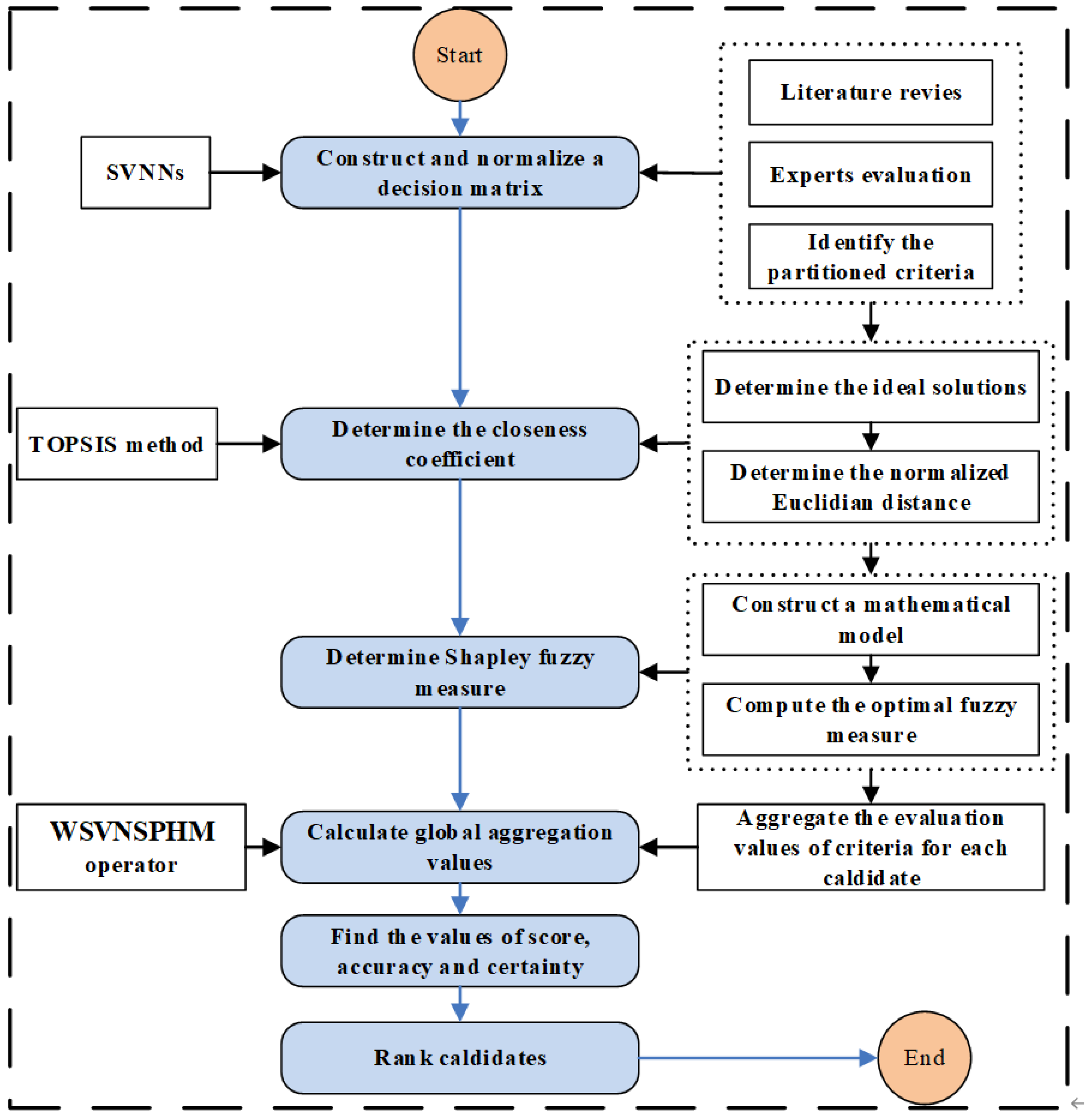
5.1. Decision-Making Process

The decision-making process, using the proposed method, is as follows.

Step 1. Construct and normalize decision matrix

The DMs assess the values as SVNNs, and criteria $c_1,c_2$, and $c_5$ belong to the cost type. The normalized decision matrix $\tilde{R}={\left({\tilde{S}}_{ij}\right)}_{n\times m}$ is obtained as shown in

Table 2. Normalized decision matrix.

	$c_1$	$c_2$	$c_3$	$c_4$	$c_5$
${\tilde{S}}_1$	<0.6,0.1,0.2>	<0.4,0.5,0.5>	<0.5,0.3,0.4>	<0.5,0.3,0.3>	<0.5,0.4,0.6>
${\tilde{S}}_2$	<0.5,0.3,0.2>	<0.3,0.4,0.6>	<0.4,0.2,0.6>	<0.6,0.1,0.2>	<0.4,0.6,0.5>
${\tilde{S}}_3$	<0.5,0.2,0.2>	<0.5,0.4,0.4>	<0.5,0.2,0.4>	<0.4,0.1,0.3>	<0.5,0.3,0.6>
${\tilde{S}}_4$	<0.6,0.1,0.2>	<0.4,0.5,0.4>	<0.5,0.4,0.3>	<0.5,0.2,0.2>	<0.6,0.2,0.3>
${\tilde{S}}_5$	<0.6,0.1,0.1>	<0.6,0.3,0.3>	<0.4,0.6,0.5>	<0.5,0.1,0.2>	<0.4,0.6,0.5>

.

• Step 2. Compute closeness coefficients

Using Equation (17), the closeness coefficients of the candidates from the positive ideal solution are determined as given in

Table 3. Closeness coefficients of candidates.

	$c_1$	$c_2$	$c_3$	$c_4$	$c_5$
${\tilde{S}}_1$	0.6259	0.7101	0.3090	0.2743	0.7101
${\tilde{S}}_2$	0.8305	0.8334	1	0.4415	0
${\tilde{S}}_3$	0.5119	0.3660	0.6340	0.1791	0.5279
${\tilde{S}}_4$	0	0.5729	0.3090	0.3483	0.4495
${\tilde{S}}_5$	0.8305	0	0	0.8209	0.2899

.

Step 3. Determine Shapley fuzzy measures

Since the five criteria are partitioned into two categories, $P_1=\left\{c_1,c_2,c_5\right\}$ and $P_2=\left\{c_3,c_4\right\}$, their optimal Shapley fuzzy measures can be determined separately. For $P_1=\left\{c_1,c_2,c_5\right\}$, we have:

$$\begin{array}{l}\min -0.1262\mu \left(c_1\right)+0.1262\mu \left(c_2,c_5\right)+0.0210\mu \left(c_1,c_5\right)-0.0210\mu \left(c_2\right)-0.1472\mu \left(c_1,c_2\right)\\ 0.1472\mu \left(c_5\right)+2.5044\\ s.t.\{\begin{array}{l}\mu \left(c_1,c_2,c_5\right)=1\\ \mu \left(E\right)\le \mu \left(F\right),\forall E,F\in CandE\subseteq F\\ 0.35\le \mu \left(c_1\right)\le 0.40\\ 0.30\le \mu \left(c_2\right)\le 0.50\\ 0.25\le \mu \left(c_5\right)\le 0.35\end{array}\end{array}$$

The above model can be solved using MATLAB software, and the fuzzy measures on the basis of the criteria are $\mu \left(c_1\right)=\mu \left(c_1,c_5\right)=0.4$, $\mu \left(c_1,c_2\right)=\mu \left(c_1,c_2,c_5\right)=1$, $\mu \left(c_2\right)=\mu \left(c_2,c_5\right)=0.30$, and $\mu \left(c_5\right)=0.25$. From Equation (1), the Shapley fuzzy measures are found to be ${\tau }_1\left(\mu ,P_1\right)=0.5083$, ${\tau }_2\left(\mu ,P_1\right)=0.4083$, and ${\tau }_3\left(\mu ,P_1\right)=0.0833$.

Similarly, the optimal Shapley fuzzy measures based on the criteria partition $P_2=\left\{c_3,c_4\right\}$ can be determined as ${\tau }_4\left(\mu ,P_2\right)=0.325$ and ${\tau }_5\left(\mu ,P_2\right)=0.675$.

Step 4. Find global aggregation values

By using the WSVNSPHM operator, i.e., Equation (12), when $p=q=1$, the global aggregation value ${\varsigma }_i\left(i=1,2,\dots ,n\right)$ of candidate $S_i\left(i=1,2,\dots ,n\right)$ can be obtained as:

$$\begin{array}{cc}\hfill {\varsigma }_1=& \langle 0.1572,0.7223,0.7720\rangle ;{\varsigma }_2=\langle 0.1186,0.7795,0.7869\rangle ;{\varsigma }_3=\langle 0.1558,0.7403,0.7500\rangle ;{\varsigma }_4=\langle 0.1602,\hfill \\ \hfill & 0.7130,0.7403\rangle ;{\varsigma }_5=\langle 0.1973,0.6796,0.6771\rangle .\hfill \end{array}$$

Step 5. Compute values of score, accuracy, and certainty

Using Definition 10, the values of score $\overline{s}\left({\varsigma }_i\right)$ are obtained as $\overline{s}\left({\varsigma }_1\right)=0.2210$;$\overline{s}\left({\varsigma }_2\right)=0.1841;\overline{s}\left({\varsigma }_3\right)=0.2218;\overline{s}\left({\varsigma }_4\right)=0.2356;\overline{s}\left({\varsigma }_5\right)=0.2802$. Since the values are not identical to each other, it is not necessary to calculate the values of the accuracy $\overline{a}\left({\varsigma }_i\right)$, and certainty $\overline{c}\left({\varsigma }_i\right)$.

Step 6. Rank candidates

Since $\overline{s}\left({\varsigma }_5\right)>\overline{s}\left({\varsigma }_4\right)>\overline{s}\left({\varsigma }_3\right)>\overline{s}\left({\varsigma }_1\right)>\overline{s}\left({\varsigma }_2\right)$, the final rank order is $S_5\succ S_4\succ S_3\succ S_1\succ S_2$ and the highest ranked is $S_5$.

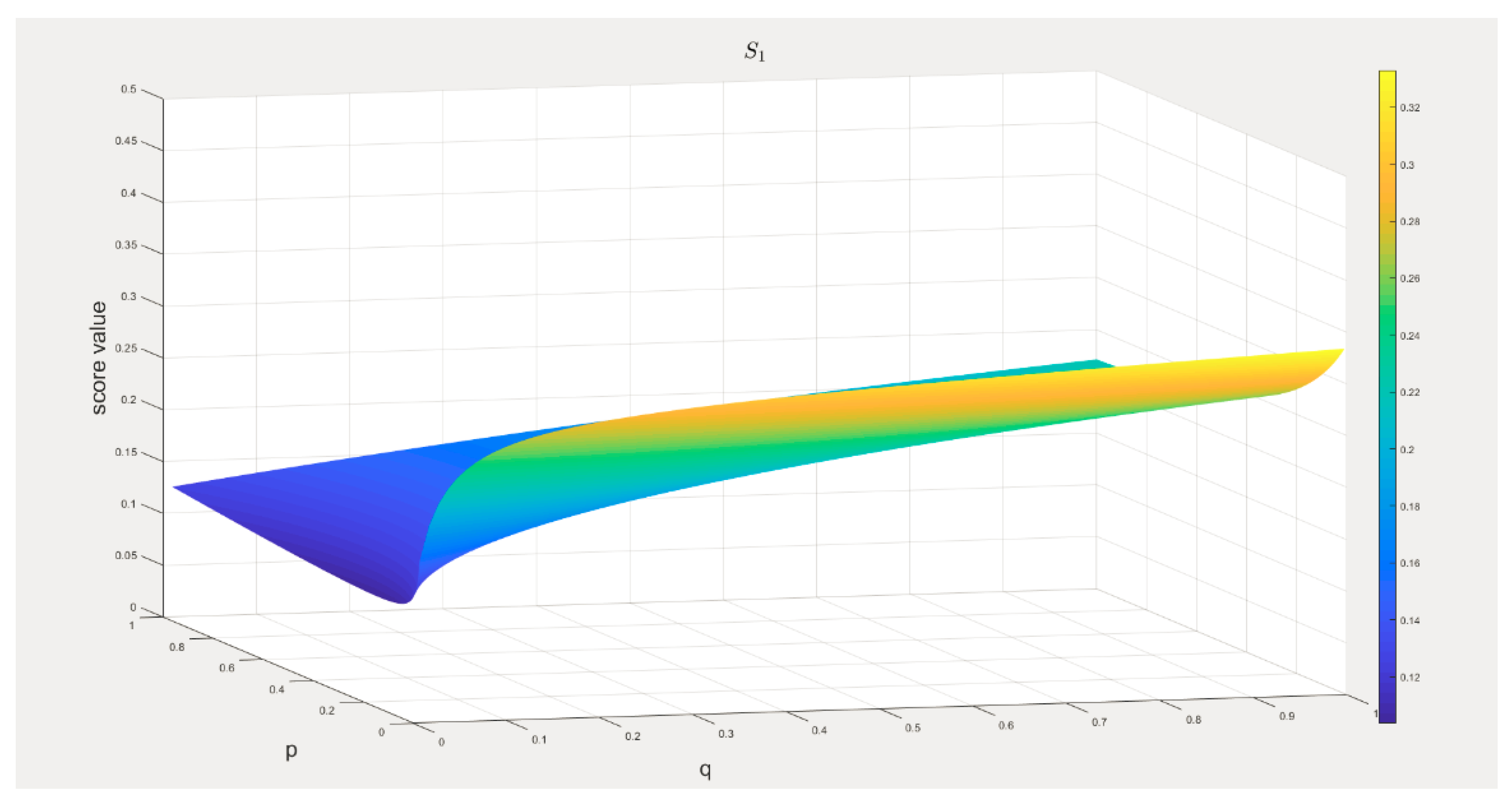
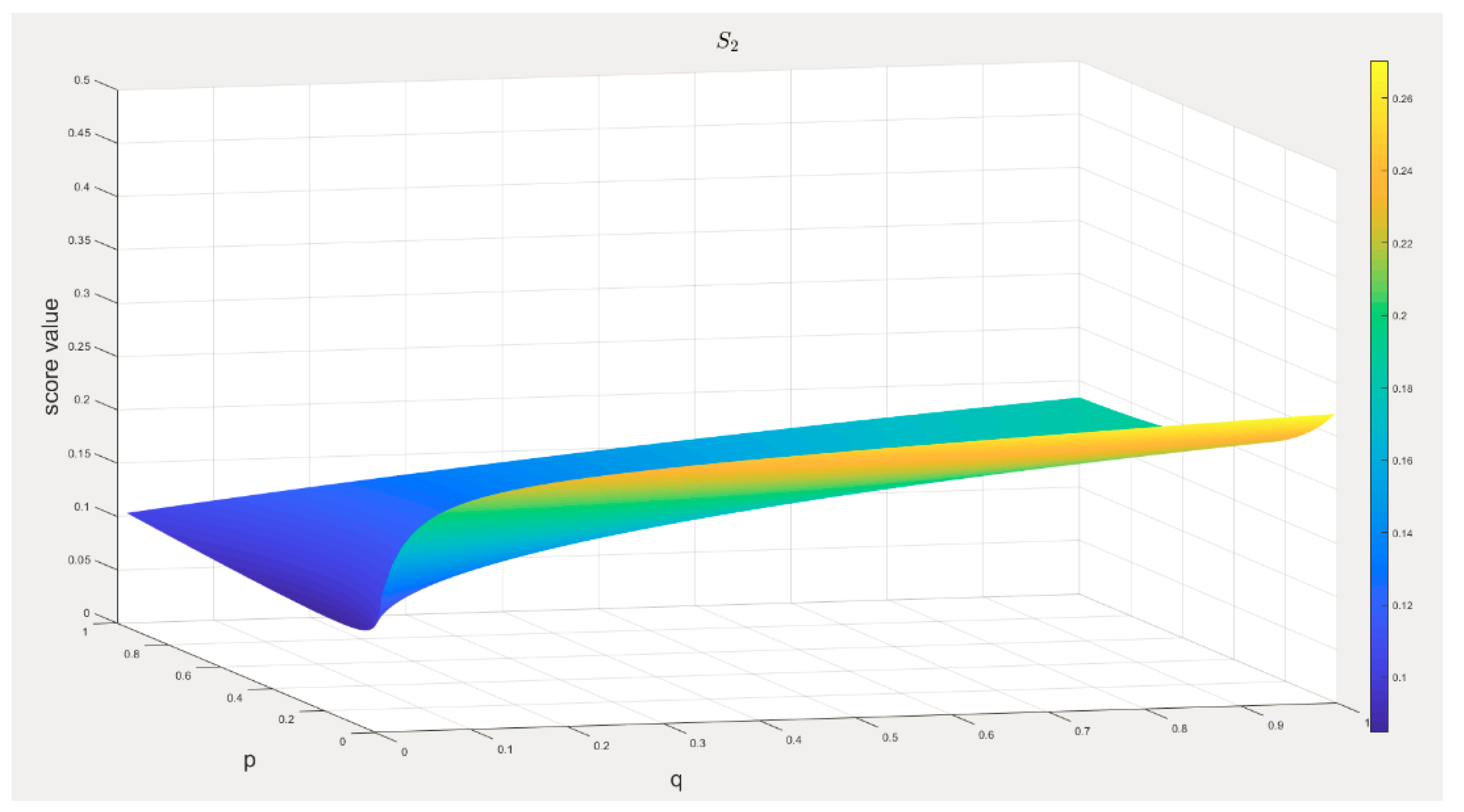
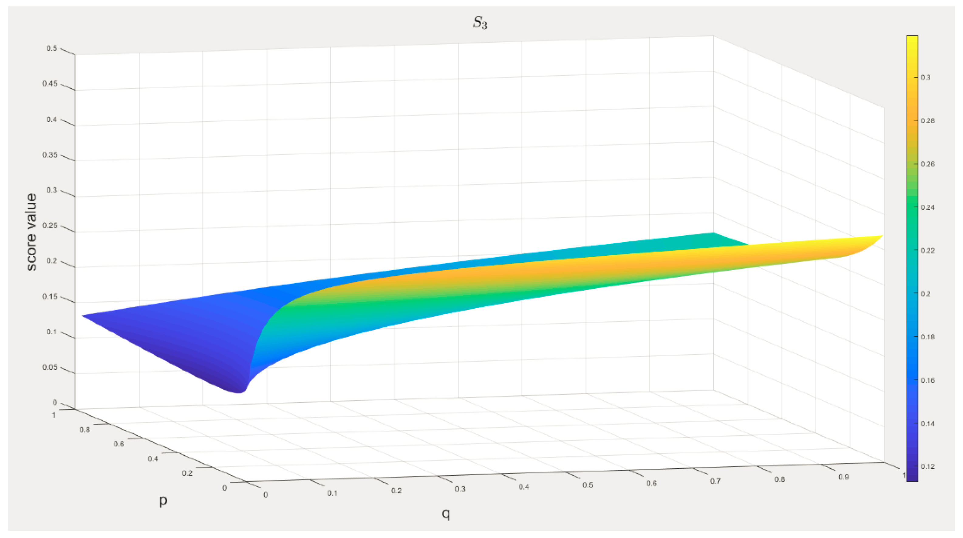
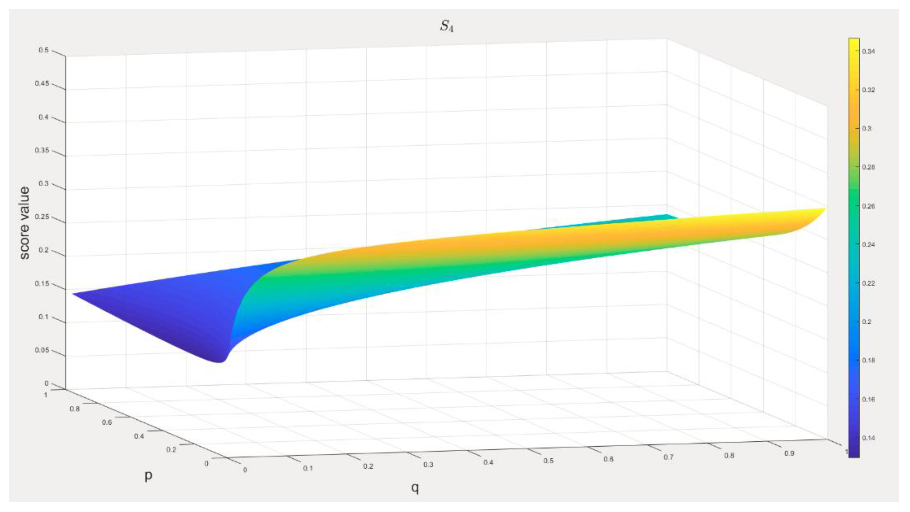
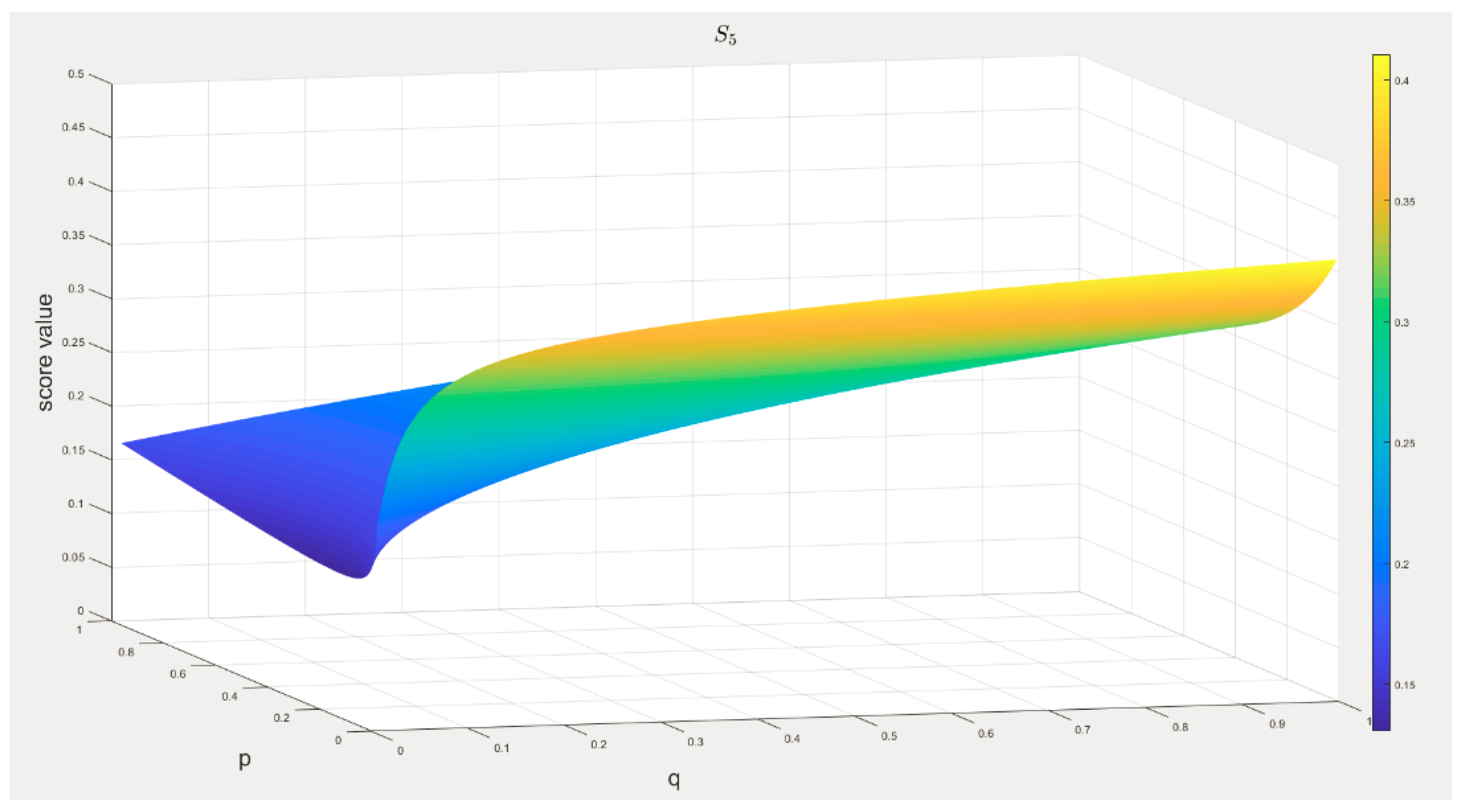
5.2. Sensitivity Analysis

Next, a sensitivity analysis can be conducted to investigate the influence of the values of $p$ and $q$ on the final rankings.

Table 4. Score values using WSVNPHM operator.

Parameter	Score Value					Final Rank Order
	$S_1$	$S_2$	$S_3$	$S_4$	$S_5$
$p=q=1$	0.2210	0.1841	0.2218	0.2354	0.2802	$S_5\succ S_4\succ S_3\succ S_1\succ S_2$
$p=q=2$	0.2741	0.2288	0.2654	0.2823	0.3371	$S_5\succ S_4\succ S_1\succ S_3\succ S_2$
$p=q=4$	0.3333	0.2759	0.3120	0.3388	0.3939	$S_5\succ S_4\succ S_1\succ S_3\succ S_2$
$p=q=6$	0.3627	0.2986	0.3357	0.3679	0.4232	$S_5\succ S_4\succ S_1\succ S_3\succ S_2$
$p=q=8$	0.3796	0.3116	0.3497	0.3848	0.4410	$S_5\succ S_4\succ S_1\succ S_3\succ S_2$
$p=q=10$	0.3905	0.3200	0.3588	0.3957	0.4528	$S_5\succ S_4\succ S_1\succ S_3\succ S_2$

shows the score values of the five candidates using the WSVNPHM operator. As can be seen, if $p=q=1$, the final rank order is $S_5\succ S_4\succ S_3\succ S_1\succ S_2$. However, when $p$ and $q$ are equal to the other values, the final rank order is $S_5\succ S_4\succ S_1\succ S_3\succ S_2$. Although the rank positions of $S_1$ and $S_3$ will change with $p$ and $q$, the best candidate is always $S_5$ while the worst is $S_2$. Table 4 shows that the gap between the first and second rank positions increases with $p$ and $q$, demonstrating the choice of candidate $S_5$ as an optimal scheme. Figure 2, Figure 3, Figure 4, Figure 5 and Figure 6 show how the score values of the five candidates change with $p$ and $q$ in the interval $[0,1]$ under the WSVNPHM operator.

5.3. Comparison Analysis

To further validate the proposed MCDM method, we compared it against some of the existing methods based on aggregation operators. Since most methods cannot handle cases when there is only partial information on the weights of the criteria, the weights were first set as $w={\left(0.5083,0.4083,0.3250,0.6750,0.0833\right)}^T$ using the optimal Shapley fuzzy measure found in Section 5.1.

For the proposed MCDM method, the weights found can be used to aggregate the preference information in Step 4 with $p=q=1$. For the MCDM methods based on the Frank aggregation [24], Hamacher [25], and Bonferroni mean [27,28] operators, the corresponding parameters are determined as $\lambda =2$ and $p=q=1$, respectively.

Table 5. Comparison results.

Source	Aggregation Operator	Interrelationship	Partition	Rank Order
Ye [22]	Algebraic	No	No	$S_4\succ S_5\succ S_3\succ S_2\succ S_1$
Peng et al. [23]	Einstein	No	No	$S_4\succ S_5\succ S_3\succ S_1\succ S_2$
Garg [24]	Frank ($\lambda =2$)	No	No	$S_5\succ S_4\succ S_3\succ S_1\succ S_2$
Liu et al. [25]	Hamacher ($\lambda =2$)	No	No	$S_4\succ S_5\succ S_3\succ S_1\succ S_2$
Liu and Wang [27]	Weighted Bonferroni mean ($p=q=1$)	Yes	No	$S_5\succ S_4\succ S_3\succ S_2\succ S_1$
Ji et al. [28]	Frank prioritized Bonferroni mean ($p=q=1,\lambda =2$)	Yes	No	$S_5\succ S_4\succ S_3\succ S_1\succ S_2$
Our method	WSVNSPHM ($p=q=1$)	Yes	Yes	$S_5\succ S_4\succ S_3\succ S_1\succ S_2$

shows the comparison results of the different methods used. Clearly, the final results found through the proposed method are the same as those by the methods employed in [24,27,28], and the best candidate is $S_5$. However, for the methods employed in [22,23,25], the best candidate is $S_4$. Notably, while the methods in [24,27,28] yield reasonable results, they do not factor in the correlation or the categories of the selection criteria. Furthermore, as discussed in [23], the rules of the corresponding operations in [22] are unreasonable, which leads to unreasonable algebraic operators. In actual decision-making instances, not all selection criteria correlate with each other. Our method can partition the criteria into distinct categories, considering not only the interrelationship of the criteria but also the independence of the criteria.

6. Conclusions

A single-valued neutrosophic MCDM problem with interdependent characteristics was investigated in this paper. Through the PHM operator and Shapley fuzzy measure, the SVNPHM and WSVNSPHM aggregation operators were defined, and their corresponding properties were discussed. An integrated MCDM method was then developed to solve single-valued neutrosophic problems where the weights of the selection criteria may not be completely known a priori. A mathematical programming model based on fuzzy measures was formed to obtain the optimal Shapley fuzzy measure. Next, the aggregation operators were used to aggregate DMs’ preference information. Finally, an example was presented to validate the proposed method, yielding reasonable outcomes. Thus, our proposed aggregation operators recognize the correlation of the selection criteria, unlike previous techniques. In future, other aggregation operators of SVNNs based on the Shapley fuzzy measure can be studied.

References

1. Zadeh, L. Fuzzy sets. Inf. Control. 1965, 8, 338–353. [Google Scholar] [CrossRef] [Green Version]
2. Wang, L.; Wang, X.-K.; Peng, J.J.; Wang, J.Q. The differences in hotel selection among various types of travellers: A comparative analysis with a useful bounded rationality behavioural decision support model. Tour. Manag. 2020, 76, 103961. [Google Scholar] [CrossRef]
3. Shen, K.-W.; Wang, X.-K.; Qiao, D.; Wang, J.-Q. Extended Z-MABAC method based on regret theory and directed distance for regional circular economy development program selection with Z-information. IEEE Trans. Fuzzy Syst. 2019. [Google Scholar] [CrossRef]
4. Peng, J.J.; Tian, C.; Zhang, W.Y.; Zhang, S.; Wang, J.Q. An integrated multi-criteria decision-making framework for sustainable supplier selection under picture fuzzy environment. Technol. Econ. Dev. Econ. 2020, 26, 573–598. [Google Scholar] [CrossRef] [Green Version]
5. Chen, Z.-Y.; Peng, J.J.; Wang, X.K.; Zhang, H.Y.; Wang, J.-Q. Solar power station site selection: A model based on data analysis and MCGDM considering expert consensus. J. Intell. Fuzzy Syst. 2020, 1–20. [Google Scholar] [CrossRef]
6. Shen, K.-W.; Li, L.; Wang, J.-Q. Circular economy model for recycling waste resources under government participation: A case study in industrial waste water circulation in china. Technol. Econ. Dev. Econ. 2019, 26, 21–47. [Google Scholar] [CrossRef]
7. Tian, C.; Peng, J.J.; Zhang, W.Y.; Zhang, S.; Wang, J.Q. Tourism environmental impact assessment based on improved AHP and picture fuzzy PROMETHEE II methods. Technol. Econ. Dev. Econ. 2020, 26, 355–378. [Google Scholar] [CrossRef]
8. Xiao, X.; Duan, H.; Wen, J. A novel car-following inertia gray model and its application in forecasting short-term traffic flow. Appl. Math. Model. 2020. [Google Scholar] [CrossRef]
9. Rao, C.; Lin, H.; Liu, M. Design of comprehensive evaluation index system for P2P credit risk of “three rural” borrowers. Soft Comput. 2020, 24, 11493–11509. [Google Scholar] [CrossRef]
10. Liu, M.; Zeng, S.; Balezentis, T.; Streimikiene, D. Picture Fuzzy Weighted Distance Measures and their Application to Investment Selection. Amfiteatru Econ. 2019, 21, 682–695. [Google Scholar] [CrossRef]
11. Zhou, J.; Li, K.W.; Balezentis, T.; Streimikiene, D. Pythagorean fuzzy combinative distance-based assessment with pure linguistic information and its application to financial strategies of multi-national companies. Econ. Res. Ekon. Istraživanja 2020, 33, 974–998. [Google Scholar] [CrossRef]
12. Peng, H.-G.; Wang, J.-Q. Multi-criteria sorting decision making based on dominance and opposition relations with probabilistic linguistic information. Fuzzy Optim. Decis. Mak. 2020, 1–36. [Google Scholar] [CrossRef]
13. Chen, Z.Y.; Wang, X.K.; Peng, J.J.; Zhang, H.Y.; Wang, J.Q. An integrated probabilistic linguistic projection method for MCGDM based on ELECTRE III and the weighted convex median voting rule. Expert Syst. 2020. [Google Scholar] [CrossRef]
14. Atanassov, K.T. Intuitionistic fuzzy sets. Fuzzy Sets Syst. 1986, 20, 87–96. [Google Scholar] [CrossRef]
15. Wang, H.; Smarandache, F.; Zhang, Y.Q.; Sunderraman, R. Single Valued Neutrosophic Sets 2010, 4, 410–413. Available online: https://www.researchgate.net/publication/262047656_Single_valued_neutrosophic_sets (accessed on 12 June 2020).
16. Smarandache, F. A Unifying Field in Logic. Neutrosophy: Neutrosophic Probability, Set and Logic; American Research Press: Rehoboth, TX, USA, 1998. [Google Scholar]
17. Rivieccio, U. Neutrosophic logics: Prospects and problems. Fuzzy Sets Syst. 2008, 159, 1860–1868. [Google Scholar] [CrossRef]
18. Majumdar, P.; Samanta, S.K. On similarity and entropy of neutrosophic sets. J. Intell. Fuzzy Syst. 2014, 26, 1245–1252. [Google Scholar] [CrossRef] [Green Version]
19. Peng, X.; Smarandache, F. New multiparametric similarity measure for neutrosophic set with big data industry evaluation. Artif. Intell. Rev. 2020, 53, 3089–3125. [Google Scholar] [CrossRef]
20. Mandal, K.; Basu, K. Vector aggregation operator and score function to solve multi-criteria decision making problem in neutrosophic environment. Int. J. Mach. Learn. Cybern. 2019, 10, 1373–1383. [Google Scholar] [CrossRef]
21. Abdel-Baset, M.; Chang, V.; Gamal, A.; Smarandache, F. An integrated neutrosophic ANP and VIKOR method for achieving sustainable supplier selection: A case study in importing field. Comput. Ind. 2019, 106, 94–110. [Google Scholar] [CrossRef]
22. Ye, J. A multicriteria decision-making method using aggregation operators for simplified neutrosophic sets. J. Intell. Fuzzy Syst. 2014, 26, 2459–2466. [Google Scholar] [CrossRef]
23. Peng, J.-J.; Wang, J.-Q.; Wang, J.; Zhang, H.-Y.; Chen, X.-H. Simplified neutrosophic sets and their applications in multi-criteria group decision-making problems. Int. J. Syst. Sci. 2016, 47, 1–17. [Google Scholar] [CrossRef]
24. Garg, H. Novel single-valued neutrosophic decision making operators under Frank norm operations and its application. Int. J. Uncertain. Quantif. 2016, 6, 361–375. [Google Scholar]
25. Liu, P.; Chu, Y.; Li, Y.; Chen, Y. Some generalized neutrosophic number Hamacher aggregation operators and their application to group decision making. Int. J. Fuzzy Syst. 2014, 16, 242–255. [Google Scholar]
26. Tian, C.; Peng, J.J. A Multi-Criteria Decision-Making Method Based on the Improved Single-Valued Neutrosophic Weighted Geometric Operator. Mathematics 2020, 8, 1051. [Google Scholar] [CrossRef]
27. Liu, P.D.; Wang, Y.M. Multiple attribute decision-making method based on single-valued neutrosophic normalized weighted Bonferroni mean. Neural Comput. Appl. 2014, 25, 2001–2010. [Google Scholar] [CrossRef]
28. Ji, P.; Wang, J.-Q.; Zhang, H. Frank prioritized Bonferroni mean operator with single-valued neutrosophic sets and its application in selecting third-party logistics providers. Neural Comput. Appl. 2018, 30, 799–823. [Google Scholar] [CrossRef]
29. Peng, J.-J.; Wang, J.-Q.; Zhang, H.-Y.; Chen, X.-H. An outranking approach for multi-criteria decision-making problems with simplified neutrosophic sets. Appl. Soft Comput. 2014, 25, 336–346. [Google Scholar] [CrossRef]
30. Ye, J. Simplified neutrosophic harmonic averaging projection-based method for multiple attribute decision-making problems. Int. J. Mach. Learn. Cybern. 2017, 8, 981–987. [Google Scholar] [CrossRef]
31. Ferreira, F.A.F.; Meidutė-Kavaliauskienė, I. Toward a sustainable supply chain for social credit: Learning by experience using single-valued neutrosophic sets and fuzzy cognitive maps. Ann. Oper. Res. 2019, 2, 1–22. [Google Scholar] [CrossRef]
32. Tian, C.; Zhang, W.; Zhang, S.; Peng, J. An Extended Single-Valued Neutrosophic Projection-Based Qualitative Flexible Multi-Criteria Decision-Making Method. Mathematics 2019, 7, 39. [Google Scholar] [CrossRef] [Green Version]
33. Ye, J. Projection and bidirectional projection measures of single-valued neutrosophic sets and their decision-making method for mechanical design schemes. J. Exp. Theor. Artif. Intell. 2017, 29, 1–10. [Google Scholar] [CrossRef] [Green Version]
34. Sykora, S. Mathematical Means and Averages: Generalized Heronian Means; Stan’s Library: Castano Primo, Italy, 2009. [Google Scholar] [CrossRef]
35. Liu, P.; Shi, L. Some neutrosophic uncertain linguistic number Heronian mean operators and their application to multi-attribute group decision making. Neural Comput. Appl. 2017, 28, 1079–1093. [Google Scholar] [CrossRef]
36. Hamacher, H. Uber Logische Verknunpfungenn Unssharfer Aussagen Undderen Zugenhorige Bewertungsfunktione. In Progress in Cybernetics and Systems Research; Trappl, K.R., Ed.; Hemisphere: Washington, DC, USA, 1978; Volume 3, pp. 276–288. [Google Scholar]
37. Liu, P. Some Hamacher Aggregation Operators Based on the Interval-Valued Intuitionistic Fuzzy Numbers and Their Application to Group Decision Making. IEEE Trans. Fuzzy Syst. 2014, 22, 83–97. [Google Scholar] [CrossRef]
38. Wang, R.; Wang, J.; Gao, H.; Wei, G. Methods for MADM with Picture Fuzzy Muirhead Mean Operators and Their Application for Evaluating the Financial Investment Risk. Symmetry 2019, 11, 6. [Google Scholar] [CrossRef] [Green Version]
39. Liu, P.; Khan, Q.; Mahmood, T.; Hassan, N. T-Spherical Fuzzy Power Muirhead Mean Operator Based on Novel Operational Laws and Their Application in Multi-Attribute Group Decision Making. IEEE Access 2019, 7, 22613–22632. [Google Scholar] [CrossRef]
40. Maclaurin, C. A second letter to Martin Folkes, Esq.: Concerning the roots of equations, with the demonstration of other rules of algebra. Philos. Trans. R. Soc. 1730, 36, 59–96. [Google Scholar]
41. Wei, G.; Wei, C.; Wang, J.; Gao, H.; Wei, Y. Some q-rung orthopair fuzzy maclaurin symmetric mean operators and their applications to potential evaluation of emerging technology commercialization. Int. J. Intell. Syst. 2019, 34, 50–81. [Google Scholar] [CrossRef]
42. Bonferroni, C. Sulle medie multiple di potenze. Bolletino Mat. Ital. 1950, 5, 267–270. [Google Scholar]
43. Liu, P.; Liu, J. Some q-rung orthopair fuzzy Bonferroni mean operators and their application to multi-attribute group decision making. Int. J. Intell. Syst. 2018, 33, 315–347. [Google Scholar] [CrossRef]
44. Liu, P.; Wang, P. Multiple-attribute decision-making based on Archimedean Bonferroni operators of q-rung orthopair fuzzy numbers. IEEE Trans. Fuzzy Syst. 2019, 27, 834–848. [Google Scholar] [CrossRef]
45. Peng, J.; Wang, J.-Q.; Hu, J.-H.; Tian, C.; Juan-Juan, P.; Jian-Qiang, W.; Jun-Hua, H. Multi-criteria decision-making approach based on single-valued neutrosophic hesitant fuzzy geometric weighted choquet integral heronian mean operator. J. Intell. Fuzzy Syst. 2018, 35, 3661–3674. [Google Scholar] [CrossRef]
46. Saaty, T.L. Decision Making with Dependence and Feedback: The Analytic Network Process; RWS Publications: Pittsburgh, PA, USA, 1996. [Google Scholar]
47. Duleba, S. An ahp-ism approach for considering public preferences in a public transport development decision. Transport 2019, 34, 662–671. [Google Scholar] [CrossRef] [Green Version]
48. Duleba, S.; Shimazaki, Y.; Mishina, T. An analysis on the connections of factors in a public transport system by AHP-ISM. Transport 2013, 28, 404–412. [Google Scholar] [CrossRef]
49. Liu, P.; Liu, J.; Merigó, J.M. Partitioned Heronian means based on linguistic intuitionistic fuzzy numbers for dealing with multi-attribute group decision making. Appl. Soft Comput. 2018, 62, 395–422. [Google Scholar] [CrossRef]
50. Theory of Fuzzy Integrals and Its Applications. Ph.D. Thesis, Tokyo Institute of Technology, Tokyo, Japan, 1974.
51. Shapley, L.S. A Value for N-Person Game; Princeton: Princeton University Press: Princeton, NJ, USA, 1953; pp. 307–317. [Google Scholar]
52. Zhang, W.K.; Ju, Y.B.; Liu, X. Multiple criteria decision analysis based on Shapley fuzzy measures and interval-valued hesitant fuzzy linguistic numbers. Comput. Ind. Eng. 2017, 105, 28–38. [Google Scholar] [CrossRef]
53. Nie, R.-X.; Tian, Z.-P.; Wang, J.-Q.; Hu, J.-H. Pythagorean fuzzy multiple criteria decision analysis based on Shapley fuzzy measures and partitioned normalized weighted Bonferroni mean operator. Int. J. Intell. Syst. 2019, 34, 297–324. [Google Scholar] [CrossRef]
54. Grabisch, M. k-order additive discrete fuzzy measures and their representation. Fuzzy Sets Syst. 1997, 92, 167–189. [Google Scholar] [CrossRef]
55. Hwang, C.L.; Yoon, K. Multiple Attribute Decision Making: Methods and Applications: A State of the Art Survey; Springer: New York, NY, USA, 1981; pp. 1–10. [Google Scholar]
Figure 1. The flowchart of the proposed method.
Mathematics 08 01189 g001
Figure 2. Values of S 1 with p , q [ 0 , 1 ] .
Mathematics 08 01189 g002
Figure 3. Values of S 2 with p , q [ 0 , 1 ] .
Mathematics 08 01189 g003
Figure 4. Values of S 3 with p , q [ 0 , 1 ] .
Mathematics 08 01189 g004
Figure 5. Values of S 4 with p , q [ 0 , 1 ] .
Mathematics 08 01189 g005
Figure 6. Values of S 5 with p , q [ 0 , 1 ] .
Mathematics 08 01189 g006