Orhonormal Wavelet Bases on The 3D Ball Via Volume Preserving Map from the Regular Octahedron

Abstract

We construct a new volume preserving map from the unit ball ${\mathbb{B}}^3$ to the regular 3D octahedron, both centered at the origin, and its inverse. This map will help us to construct refinable grids of the 3D ball, consisting in diameter bounded cells having the same volume. On this 3D uniform grid, we construct a multiresolution analysis and orthonormal wavelet bases of $L^2\left({\mathbb{B}}^3\right)$, consisting in piecewise constant functions with small local support.

1. Introduction

Spherical 3D signals occur in a wide range of fields, including computer graphics, and medical imaging (e.g., 3D reconstruction of medical images [1]), crystallography (texture analysis of crystals) [2,3] and geoscience [4,5,6]. Therefore, we need suitable efficient techniques for manipulating such signals, and one of the most efficient technique consists in using wavelets on the 3D ball (see e.g., [4,5,6,7,8,9,10] and the references therein). In this paper we propose to construct an orthonormal basis of wavelets with small support, defined on the 3D ball ${\mathbb{B}}^3$, starting from a multiresolution analysis. Our wavelets will be piecewise constant functions on the cells of a uniform and refinable grid of ${\mathbb{B}}^3$. By a refinable (or hierarchical) grid we mean that the cells can be divided successively into a given number of smaller cells of the same volume. By a uniform grid we mean that all the cells at a certain level of subdivision have the same volume. These two very important properties of our grid derive from the fact that it is constructed by mapping a uniform and refinable grid of the 3D regular octahedron, using a volume preserving map onto ${\mathbb{B}}^3$. Compared to the wavelets on the 3D ball constructed in [8,10], with localized support, our wavelets have local support, and this is very important when dealing with data consisting in big jumps on small portions, as shown in [11]. Another construction of piecewise constant wavelets on the 3D ball was realized in [7], starting from a similar construction on the 2D sphere. The author assumes that his wavelets are the first Haar wavelets on the 3D ball which are orthogonal and symmetric, even though we do not see any symmetry, neither in the cells, nor in the decomposition matrix. Moreover, his $8\times 8$ decomposition matrices change in each step of the refinement, the entries depending on the volumes of the cells, which are, in our opinion, difficult to evaluate and for this reason they are not calculated explicitly in [7]. Another advantage of our construction is that our cells are diameter bounded, unlike the cells in [7] containing the origin, which become long and thin after some steps of refinement.

The paper is structured as follows. In Section 2 we introduce some notations used for the construction of the volume preserving map. In Section 3 we construct the volume preserving maps between the regular 3D octahedron and the 3D ball ${\mathbb{B}}^3$. In Section 4 we construct a uniform refinable grid of the regular octahedron followed by implementation issues, and its projection onto ${\mathbb{B}}^3$. Finally, in Section 5 we construct a multiresolution analysis and piecewise constant wavelet bases of $L^2\left({\mathbb{B}}^3\right)$.

2. Preliminaries

Consider the ball of radius r centered at the origin O, defined as

$${\mathbb{B}}^3=\{(x,y,z)\in {\mathbb{R}}^3,x^2+y^2+z^2\le r^2\}$$

and the regular octahedron $\mathbb{K}$ of the same volume, centered at O and with vertices on the coordinate axes

$$\mathbb{K}=\{(x,y,z)\in {\mathbb{R}}^3,\left|x\right|+\left|y\right|+\left|z\right|\le a\}.$$

Since the volume of the regular octahedron is $4a^3/3$, we have

$$a=r\sqrt[3]{\pi }.$$

(1)

The parametric equations of the ball are

$$\begin{array}{c}x=\rho cos\theta sin\phi ,\hfill \\ y=\rho sin\theta sin\phi ,\hfill \\ z=\rho cos\phi ,\hfill \end{array}$$

(2)

where $\phi \in [0,\pi ]$ is the colatitude, $\theta \in [0,2\pi )$ is the longitude and $\rho \in [0,r]$ is the distance to the origin. A simple calculation shows that the volume element of the ball is

$$dV={\rho }^{2}sin\phi d\rho d\theta d\phi .$$

(3)

The ball and the octahedron can be split into eight congruent parts (see Figure 1), each part being situated in one of the eight octants $I_i^{\pm }$, $i=0,1,2,3$,

$$\begin{array}{c}\hfill I_0^{+}=\{(x,y,z),x\ge 0,y\ge 0,z\ge 0\},I_0^{-}=\{(x,y,z),x\ge 0,y\ge 0,z\le 0\},\\ \hfill I_1^{+}=\{(x,y,z),x\le 0,y\ge 0,z\ge 0\},I_1^{-}=\{(x,y,z),x\le 0,y\ge 0,z\le 0\},\\ \hfill I_2^{+}=\{(x,y,z),x\le 0,y\le 0,z\ge 0\},I_2^{-}=\{(x,y,z),x\le 0,y\le 0,z\le 0\},\\ \hfill I_3^{+}=\{(x,y,z),x\ge 0,y\le 0,z\ge 0\},I_3^{-}=\{(x,y,z),x\ge 0,y\le 0,z\le 0\}.\end{array}$$

Let ${\mathbb{B}}_i^s$ and ${\mathbb{K}}_i^s$ be the regions of ${\mathbb{B}}^3$ and $\mathbb{K}$, situated in $I_i^s$, respectively.

Next we will construct a map $\mathcal{U}:{\mathbb{B}}^3\to \mathbb{K}$ which preserves the volume, i.e., $\mathcal{U}$ satisfies

$$\mathrm{vol}\left(D\right)=\mathrm{vol}\left(\mathcal{U}\left(D\right)\right),\mathrm{for}\mathrm{all}D\subseteq {\mathbb{B}}^3,$$

(4)

where $\mathrm{vol}\left(D\right)$ denotes the volume of a domain $D.$ For an arbitrary point $(x,y,z)\in {\mathbb{B}}^3$ we denote

$$(X,Y,Z)=\mathcal{U}(x,y,z)\in \mathbb{K}.$$

(5)

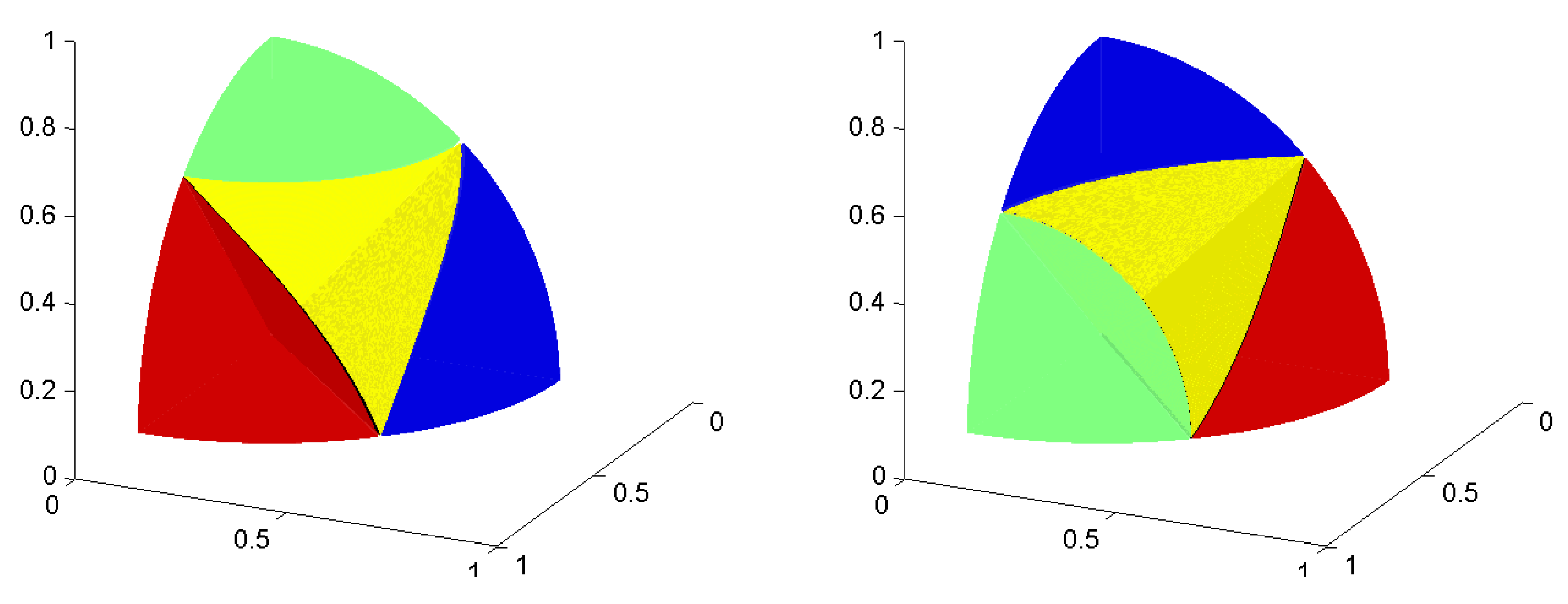
3. Construction of the Volume Preserving Map ${U}$ and Its Inverse

We focus on the region ${\mathbb{B}}_0^{+}\subset I_0^{+}$ where we consider the points $A=(r,0,0)$, $B=(0,r,0)$, $C=(0,0,r)$ and the vertical plane of equation $y=xtan\alpha$ with $\alpha \in (0,\pi /2)$ (see Figure 2 (left)). We denote by M its intersection with the great arc $\widetilde{AB}$ of the sphere of radius r. More precisely, $M=(rcos\alpha ,rsin\alpha ,0).$ The volume of the spherical region $OAMC$ equals $r^3\alpha /3.$

Now we intersect the region ${\mathbb{K}}_1^{+}$ of the octahedron with the vertical plane of equation $y=xtan\beta$ and denote by $M^{\prime }(m,n,0)$ its intersection with the edge $A^{\prime }{B}^{\prime }$, where $A^{\prime }(a,0,0),$ $B^{\prime }(0,a,0)$ (see Figure 2 (right)). Then $m+n=a$ and from $n=mtan\beta$ we find

$$m=a·\frac{1}{1+tan\beta },n=a·\frac{tan\beta }{1+tan\beta }.$$

The volume of $O{A}^{\prime }{M}^{\prime }{C}^{\prime }$ is

$$\mathcal{V}\left(O{A}^{\prime }{M}^{\prime }{C}^{\prime }\right)=\frac{O{C}^{\prime }·\mathcal{A}\left(O{A}^{\prime }{M}^{\prime }\right)}{3}=\frac{a}{3}·\frac{O{A}^{\prime }·n}{2}=\frac{a^{3}tan\beta }{6(1+tan\beta )}.$$

If we want the volume of the region $OAMC$ of the unit ball to be equal to the volume of $O{A}^{\prime }{M}^{\prime }{C}^{\prime }$, we obtain

$$\alpha =\frac{\pi }{2}·\frac{tan\beta }{1+tan\beta },\mathrm{whence}tan\beta =\frac{2\alpha }{\pi -2\alpha }.$$

This give us a first relation between $(x,y,z)$ and $(X,Y,Z)$:

$$\frac{Y}{X}=\frac{2arctan\frac{y}{x}}{\pi -2arctan\frac{y}{x}}.$$

Using the spherical coordinates (2) we obtain

$$Y=\frac{2\theta }{\pi -2\theta }·X.$$

(6)

In order to obtain a second relation between $(x,y,z)$ and $(X,Y,Z)$, we impose that, for an arbitrary $\tilde{\rho }\in (0,r]$ the region

$$\{(x,y,z)\in {\mathbb{R}}^3,x^2+y^2+z^2\le {\tilde{\rho }}^2,x,y,z\ge 0\}\mathrm{of}\mathrm{volume}\frac{\pi {\tilde{\rho }}^3}{6}$$

is mapped by $\mathcal{U}$ onto

$$\{(X,Y,Z)\in {\mathbb{R}}^3,X+Y+Z\le \ell ,X,Y,Z\ge 0\}\mathrm{of}\mathrm{volume}\frac{{\ell }^3}{6}.$$

Then, the volume preserving condition (4) implies $\ell =a·\tilde{\rho }/r$, with a satisfying (1). Thus,

$$X+Y+Z=\frac{a}{r}\sqrt{x^2+y^2+z^2}$$

and in spherical coordinates this can be written as

$$X+Y+Z=\frac{a\rho }{r}.$$

(7)

In order to have a volume preserving map, the modulus of the Jacobian $J\left(\mathcal{U}\right)$ of $\mathcal{U}$ must be 1, or, equivalently, taking into account the volume element (3), we must have

$$J\left(\mathcal{U}\right)=\left|\begin{array}{ccc}{X}_{\rho }^{\prime }& X_{\phi }^{\prime }& X_{\theta }^{\prime }\\ Y_{\rho }^{\prime }& Y_{\phi }^{\prime }& Y_{\theta }^{\prime }\\ Z_{\rho }^{\prime }& Z_{\phi }^{\prime }& Z_{\theta }^{\prime }\end{array}\right|={\rho }^{2}sin\phi .$$

(8)

Taking into account formula (7), we have

$$J\left(\mathcal{U}\right)=\left|\begin{array}{ccc}{X}_{\rho }^{\prime }& X_{\phi }^{\prime }& X_{\theta }^{\prime }\\ Y_{\rho }^{\prime }& Y_{\phi }^{\prime }& Y_{\theta }^{\prime }\\ a/r-X_{\rho }^{\prime }-Y_{\rho }^{\prime }& -X_{\phi }^{\prime }-Y_{\phi }^{\prime }& -X_{\theta }^{\prime }-Y_{\theta }^{\prime }\end{array}\right|=\left|\begin{array}{ccc}{X}_{\rho }^{\prime }& X_{\phi }^{\prime }& X_{\theta }^{\prime }\\ Y_{\rho }^{\prime }& Y_{\phi }^{\prime }& Y_{\theta }^{\prime }\\ a/r& 0& 0\end{array}\right|=\frac{a}{r}\left|\begin{array}{cc}{X}_{\phi }^{\prime }& X_{\theta }^{\prime }\\ Y_{\phi }^{\prime }& Y_{\theta }^{\prime }\end{array}\right|.$$

Further, using relation (6) we get

$$J\left(\mathcal{U}\right)=\frac{a}{r}\left|\begin{array}{cc}{X}_{\phi }^{\prime }& X_{\theta }^{\prime }\\ \frac{2\theta }{\pi -2\theta }·X_{\phi }^{\prime }& \frac{2\theta }{\pi -2\theta }·X_{\theta }^{\prime }+\frac{2\pi }{{(\pi -2\theta )}^2}·X\end{array}\right|=\frac{a}{r}\left|\begin{array}{cc}{X}_{\phi }^{\prime }& X_{\theta }^{\prime }\\ 0& \frac{2\pi }{{(\pi -2\theta )}^2}·X\end{array}\right|=\frac{2\pi a}{r{(\pi -2\theta )}^2}X{X}_{\phi }^{\prime }.$$

For the last equality, we have multiplied the first row by $-2\theta /(\pi -2\theta )$ and we have added it to the second row. Then, using the expression for $J\left(\mathcal{U}\right)$ obtained in (8) we get the differential equation

$$2X_{\phi }^{\prime }·X=\frac{r{\rho }^2}{\pi a}{(\pi -2\theta )}^{2}sin\phi .$$

The integration with respect to $\phi$ gives

$$X^2=-\frac{r{(\pi -2\theta )}^2}{\pi a}{\rho }^{2}cos\phi +\mathcal{C}(\theta ,\rho ),$$

and further, for finding $\mathcal{C}(\theta ,\rho )$ we use the fact that, for $\phi =\pi /2$ we must obtain $Z=0$. Thus, for $\phi =\pi /2$ we have

$$\begin{gathered} X^2=\mathcal{C}(\theta ,\rho ),\mathrm{so}Y=\frac{2\theta }{\pi -2\theta }\sqrt{\mathcal{C}(\theta ,\rho )},\mathrm{and} \\ Z=\frac{a\rho }{r}-X-Y=\frac{a\rho }{r}-\frac{\pi }{\pi -2\theta }\sqrt{\mathcal{C}(\theta ,\rho )}. \end{gathered}$$

Thus, $Z=0$ is obtained for

$$\mathcal{C}(\theta ,\rho )=\frac{a^2{\rho }^2}{{\pi }^2{r}^2}{(\pi -2\theta )}^2,$$

and finally, the map $\mathcal{U}$ restricted to the region $I_0^{+}$ is

$$\begin{array}{cc}\hfill X& =\frac{\sqrt{2}}{{\pi }^{2/3}}·\rho (\pi -2\theta )sin\frac{\phi }{2},\hfill \end{array}$$

(9)

$$\begin{array}{cc}\hfill Y& =\frac{\sqrt{2}}{{\pi }^{2/3}}·\rho ·2\theta sin\frac{\phi }{2},\hfill \end{array}$$

(10)

$$\begin{array}{cc}\hfill Z& ={\pi }^{1/3}\rho (1-\sqrt{2}sin\frac{\phi }{2}).\hfill \end{array}$$

(11)

In the other seven octants, the map $\mathcal{U}$ can be obtained by symmetry as follows. A point $(x,y,z)\in {\mathbb{B}}^3,$ can be written as

$$(x,y,z)=(sgn\left(x\right)·|x|,sgn\left(y\right)·|y|,sgn\left(z\right)·|z\left|\right),\mathrm{with}\left(\right|x|,|y|,|z\left|\right)\in I_0^{+}.$$

Therefore, if we denote by $(\overline{X},\overline{Y},\overline{Z})=\mathcal{U}\left(\right|x|,|y|,|z\left|\right)$, then we can define $\mathcal{U}(x,y,z)$ as

$$\mathcal{U}(x,y,z)=(sgn\left(x\right)·\overline{X},sgn\left(y\right)·\overline{Y},sgn\left(z\right)·\overline{Z}).$$

(12)

Next we deduce the formulas for the inverse of $\mathcal{U}$. First, from (6) we obtain

$$\theta =\frac{\pi Y}{2(X+Y)},$$

and from (7) we have

$$\rho =\frac{r}{a}(X+Y+Z)={\pi }^{-1/3}(X+Y+Z).$$

Adding (9) and (10), after some more calculations we obtain

$$sin\frac{\phi }{2}=\frac{X+Y}{\sqrt{2}(X+Y+Z)},$$

and further

$$cos\phi =\frac{Z(2X+2Y+Z)}{{(X+Y+Z)}^2},sin\phi =\frac{X+Y}{X+Y+Z}\sqrt{2-{\left(\frac{X+Y}{X+Y+Z}\right)}^2}.$$

Finally, the inverse ${\mathcal{U}}^{-1}:\mathbb{K}\to {\mathbb{B}}^3$ is defined by

$$\begin{array}{cc}\hfill x& ={\pi }^{-1/3}(X+Y)\sqrt{2-{\left(\frac{X+Y}{X+Y+Z}\right)}^2}cos\frac{\pi Y}{2(X+Y)},\hfill \end{array}$$

(13)

$$\begin{array}{cc}\hfill y& ={\pi }^{-1/3}(X+Y)\sqrt{2-{\left(\frac{X+Y}{X+Y+Z}\right)}^2}sin\frac{\pi Y}{2(X+Y)},\hfill \end{array}$$

(14)

$$\begin{array}{cc}\hfill z& ={\pi }^{-1/3}\frac{Z(2X+2Y+Z)}{(X+Y+Z)}.\hfill \end{array}$$

(15)

for $(X,Y,Z)\in {\mathbb{K}}_0^{+}$, and for the other seven octants the formulas can be calculated as in (12).

4. Uniform and Refinable Grids of the Regular Octahedron and of the Ball

In this section we construct a uniform refinement of the regular octahedron $\mathbb{K}$ of volume $\mathrm{vol}\left(\mathbb{K}\right)$, more precisely a subdivision of $\mathbb{K}$ into 64 cells of two shapes, each of them having the volume $\mathrm{vol}\left(\mathbb{K}\right)/64$. This subdivision can be repeated for each of the 64 small cells, the resulting ${64}^2$ cells of volume $\mathrm{vol}\left(\mathbb{K}\right)/{64}^2$ being of one of the two types from the first refinement. Next, the volume preserving map $\mathcal{U}$ will allow us the construction of uniform and refinable grids of the 3D ball ${\mathbb{B}}^3$ by transporting the octahedral uniform refinable 3D grids, and further, the construction of orthonormal piecewise constant wavelets on the 3D ball.

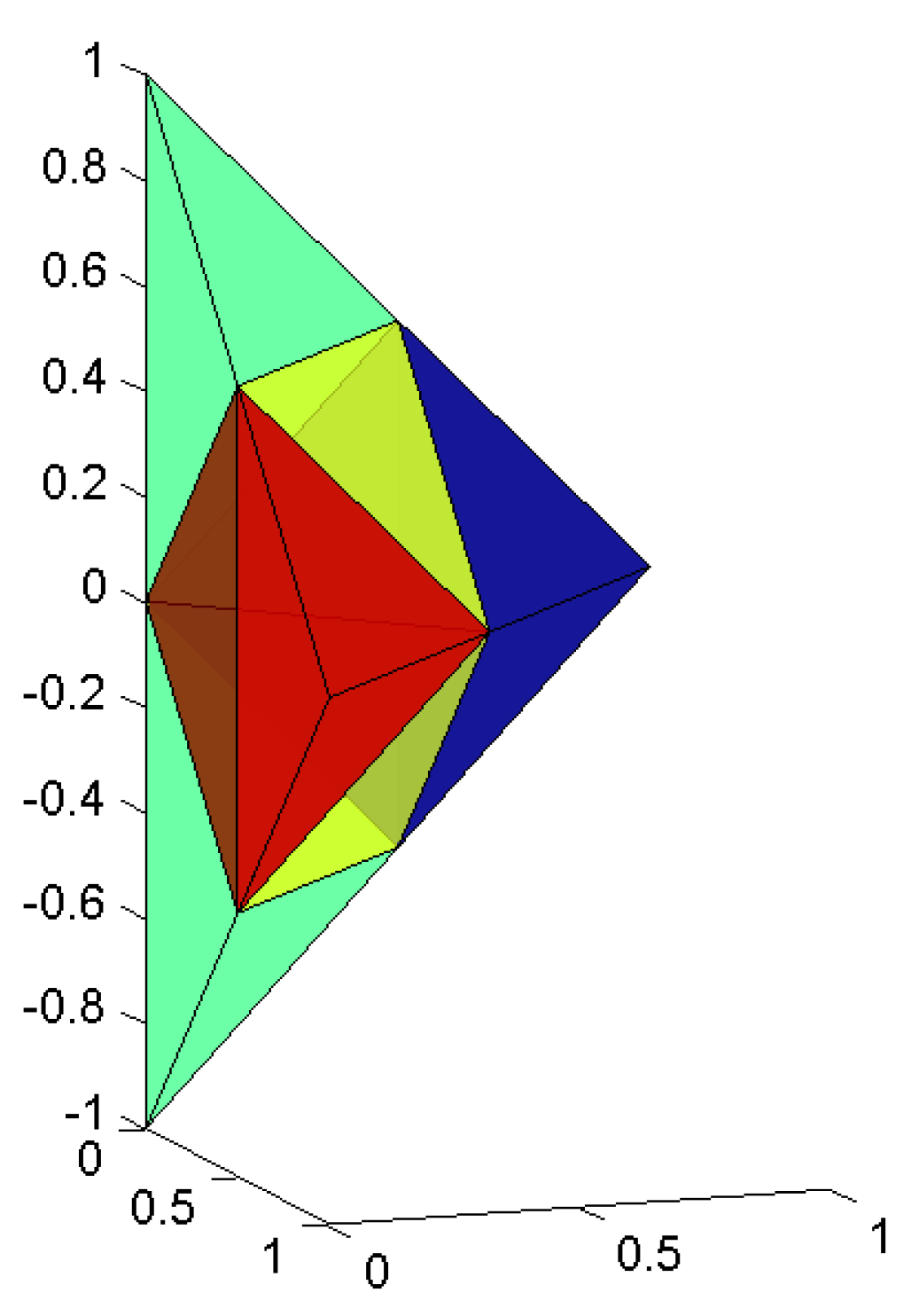
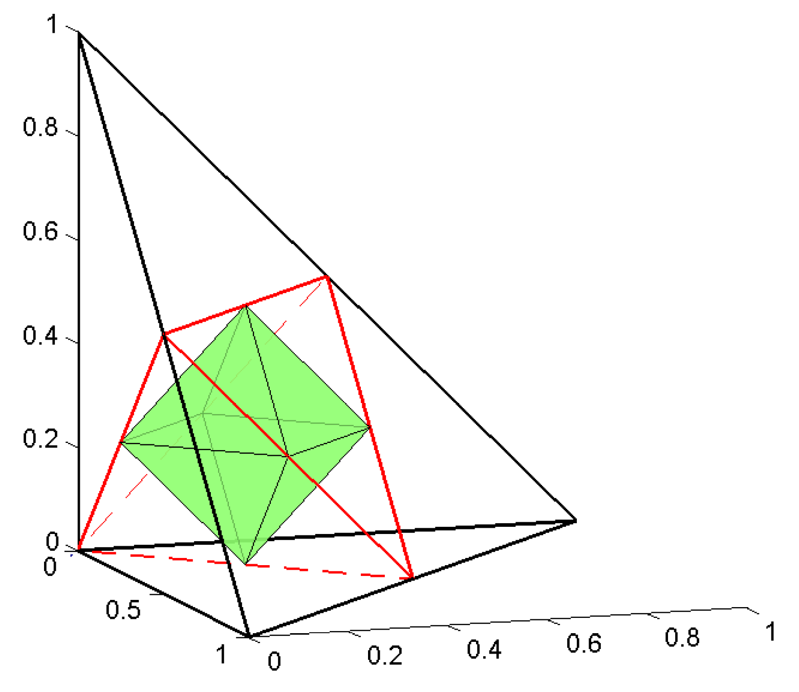
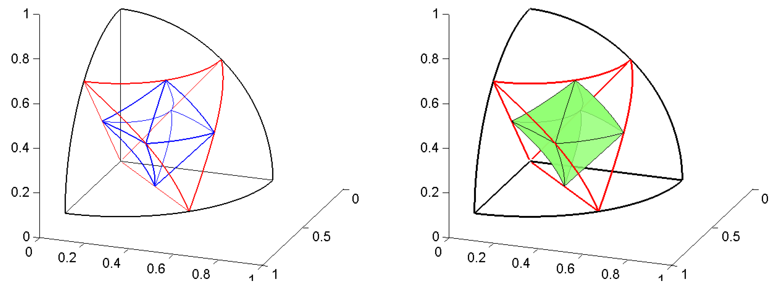
4.1. Refinement of the Octahedron

The initial octahedron $\mathbb{K}$ consists in four congruent cells, each situated in one of the octants $I_i^{+}\cup I_i^{-}$, $i=0,1,2,3$ (see Figure 3). We will say that this type of cell is ${\mathbf{T}}_0$, the index 0 of ${\mathbf{T}}_0$ being the coarsest level of the refinement. For simplifying the writing we denote by ${\mathbb{N}}_0$ the set of positive natural numbers and by ${\mathbb{N}}_n=\{1,2,\dots ,n\}$, for $n\in {\mathbb{N}}_0$.

4.1.1. First Step of Refinement

The cell ${\mathbf{T}}_0=\left(ABCD\right)\in I_0^{+}\cup I_0^{-}$, with $A(a,0,0)$, $B(0,a,0)$, $C(0,0,a)$, $D(0,0,-a)$ (see Figure 3), will be subdivided into eight smaller cells having the same volume, as follows: we take the mid-points $M,N,P,Q,R$ of the edges $AC$, $BC$, $AB$, $AD$, $BD$, respectively. Thus, one obtains $t_1=6$ cells of type ${\mathbf{T}}_1$ ($MQOP$, $MQAP$, $NROP$, $NRBP$, $ODQR$ and $COMN$), and $m_1=2$ other cells, $OMNP$ and $OPQR$, of another type, say ${\mathbf{M}}_1$. The cells of type ${\mathbf{T}}_1$ have the same shape with the cells ${\mathbf{T}}_0$. Their volumes are

$$\mathrm{vol}\left({\mathbf{T}}_1\right)=\mathrm{vol}\left({\mathbf{M}}_1\right)=\frac{\mathrm{vol}\left({\mathbf{T}}_0\right)}{8}.$$

Figure 4 and Figure 5 also show the eight cells at the first step of refinement.

Similarly we refine the other three cells situated in $I_i^{+}\cup I_i^{-}$, $i=1,2,3$, therefore the total number of cells after the first step of refinement is 32, more precisely 24 of type ${\mathbf{T}}_1$ and 8 of type ${\mathbf{M}}_1.$

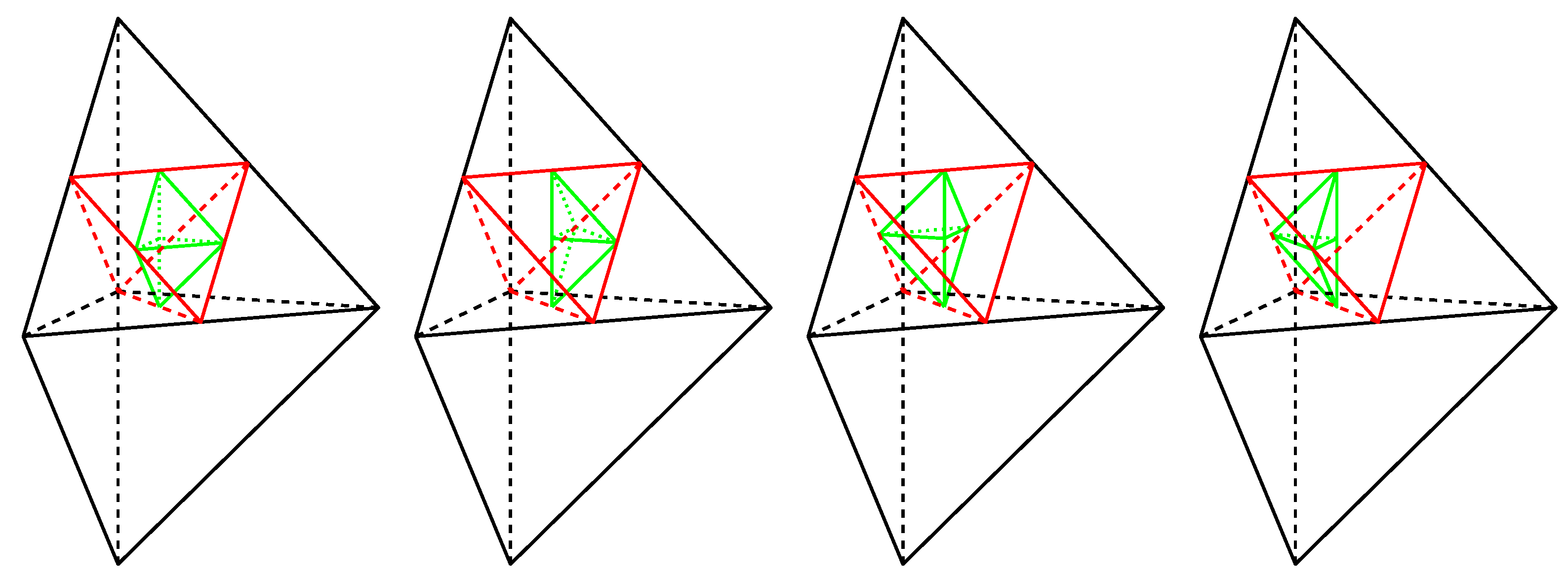
4.1.2. Second Step of Refinement

A cell of type ${\mathbf{T}}_1$ will be subdivided in the same way as a cell of type ${\mathbf{T}}_0$, i.e., into six cells of type ${\mathbf{T}}_2$ and two cells of type ${\mathbf{M}}_2$. Their volumes will be

$$\mathrm{vol}\left({\mathbf{T}}_2\right)=\mathrm{vol}\left({\mathbf{M}}_2\right)=\frac{\mathrm{vol}\left({\mathbf{T}}_0\right)}{8^2}.$$

Therefore, from the subdivision of the 6 cells of type ${\mathbf{T}}_1$ we have 36 cells of type ${\mathbf{T}}_2$ and 12 cells of type ${\mathbf{M}}_2$.

For a cell $\left(OMNP\right)$ of type ${\mathbf{M}}_1$, which is a regular tetrahedron of edge ${\ell }_1=a\sqrt{2}/2$, we take the mid-points of the six edges (see Figure 6 and Figure 7). This will give four cells of type ${\mathbf{T}}_2$ in the middle and four cells of type ${\mathbf{M}}_2$, i.e., regular tetrahedrons of edge ${\ell }_2=a\sqrt{2}/2^2$. From the subdivision of the two cells of type ${\mathbf{M}}_1$ we have 8 cells of type ${\mathbf{T}}_2$ and 8 cells of type ${\mathbf{M}}_2$.

In conclusion, the second step of subdivision yields in $I_0^{+}\cup I_0^{-}$ $t_2=44$ cells of type ${\mathbf{T}}_2$ and $m_2=20$ cells of type ${\mathbf{M}}_2$, each having the volume $\mathrm{vol}\left({\mathbf{T}}_0\right)/64,$ therefore the total number of cells after the second refinement will be $4·8^2$, more precisely 76 of type ${\mathbf{T}}_2$ and 80 of type ${\mathbf{M}}_2$.

4.1.3. The General Step of Refinement

Let $m_j$ and $t_j$ denote the numbers of cells of type ${\mathbf{M}}_j$ and ${\mathbf{T}}_j$, respectively, resulted at the step j of the subdivision, starting from one cell of type $T_0$. At this step, each of the $t_{j-1}$ cells of type ${\mathbf{T}}_{j-1}$ is subdivided into 6 cells of type ${\mathbf{T}}_j$ and 2 cells of type ${\mathbf{M}}_j$, and each of the $m_{j-1}$ cells of type ${\mathbf{M}}_{j-1}$ is subdivided into 4 cells of type ${\mathbf{T}}_j$ and 4 cells of type ${\mathbf{M}}_j.$ This implies

$$\begin{array}{c}\hfill t_j=6t_{j-1}+4m_{j-1},\\ \hfill m_j=2t_{j-1}+4m_{j-1},\end{array}$$

or

$$\left(\begin{array}{c}{t}_j\\ m_j\end{array}\right)=A\left(\begin{array}{c}{t}_{j-1}\\ m_{j-1}\end{array}\right)=A^2\left(\begin{array}{c}{t}_{j-2}\\ m_{j-2}\end{array}\right)=\dots =A^j\left(\begin{array}{c}{t}_0\\ m_0\end{array}\right),$$

with $t_0=1$, $m_0=0$ and $A=\left(\begin{array}{cc}6& 4\\ 2& 4\end{array}\right).$ After some calculations we obtain

$$\begin{gathered} A^j=\frac{1}{3}\left(\begin{array}{cc}{2}^j(2^{2j+1}+1)& 2^{j+1}(2^{2j}-1)\\ 2^j(2^{2j}-1)& 2^j(2^{2j}+2)\end{array}\right),\mathrm{whence} \\ {t}_j=\frac{2^j}{3}(2^{2j+1}+1),m_j=\frac{2^j}{3}(2^{2j}-1), \end{gathered}$$

the total number of cells of ${\mathbb{K}}_1^{+}\cup {\mathbb{K}}_1^{-}$ at step j being $t_j+m_j=8^j,$ and $4·8^j$ for the whole octahedron $\mathbb{K}$. Each of the cells of type ${\mathbf{T}}_j$ and ${\mathbf{M}}_j$ has the volume $\mathrm{vol}\left({\mathbf{T}}_0\right)/8^j.$

4.2. Implementation Issues

Every cell of the polyhedron is identified by the coordinates of its four vertices. We have two types of cells, which will be denoted by $\mathbf{T}$ and $\mathbf{M}$.

A cell of type $\mathbf{T}$ has the same coordinates x and y for the first two vertices. The z coordinate of the first vertex is greater than the z coordinate of the second vertex and the mean value of these z coordinates gives the value of the z coordinate of the third and fourth vertices of $\mathbf{T}$.

A cell of type $\mathbf{M}$ has two pairs of vertices at the same altitude (the same value of the z coordinate).

At every step of refinement, every cell $\mathbf{T}$ is divided into 6 cells of type $\mathbf{T}$ and two cells of type $\mathbf{M}$. Suppose $[{\mathbf{p}}_1,{\mathbf{p}}_2,{\mathbf{p}}_3,{\mathbf{p}}_4]$ is the array giving the coordinates of the four vertices of a T cell. The coordinates of the vertices of the next level cells are computed as follows

$$\begin{array}{cc}\hfill \mathrm{next}\mathrm{level}\mathrm{cell}\mathrm{number}1:& \frac{1}{2}[{\mathbf{p}}_1+{\mathbf{p}}_1,{\mathbf{p}}_1+{\mathbf{p}}_2,{\mathbf{p}}_1+{\mathbf{p}}_3,{\mathbf{p}}_1+{\mathbf{p}}_4],\hfill \\ \hfill \mathrm{next}\mathrm{level}\mathrm{cell}\mathrm{number}2:& \frac{1}{2}[{\mathbf{p}}_2+{\mathbf{p}}_1,{\mathbf{p}}_2+{\mathbf{p}}_2,{\mathbf{p}}_2+{\mathbf{p}}_3,{\mathbf{p}}_2+{\mathbf{p}}_4],\hfill \\ \hfill \mathrm{next}\mathrm{level}\mathrm{cell}\mathrm{number}3:& \frac{1}{2}[{\mathbf{p}}_3+{\mathbf{p}}_1,{\mathbf{p}}_3+{\mathbf{p}}_2,{\mathbf{p}}_3+{\mathbf{p}}_3,{\mathbf{p}}_3+{\mathbf{p}}_4],\hfill \\ \hfill \mathrm{next}\mathrm{level}\mathrm{cell}\mathrm{number}4:& \frac{1}{2}[{\mathbf{p}}_4+{\mathbf{p}}_1,{\mathbf{p}}_4+{\mathbf{p}}_2,{\mathbf{p}}_4+{\mathbf{p}}_3,{\mathbf{p}}_4+{\mathbf{p}}_4],\hfill \\ \hfill \mathrm{next}\mathrm{level}\mathrm{cell}\mathrm{number}5:& \frac{1}{2}[{\mathbf{p}}_1+{\mathbf{p}}_3,{\mathbf{p}}_2+{\mathbf{p}}_3,{\mathbf{p}}_3+{\mathbf{p}}_4,{\mathbf{p}}_1+{\mathbf{p}}_2],\hfill \\ \hfill \mathrm{next}\mathrm{level}\mathrm{cell}\mathrm{number}6:& \frac{1}{2}[{\mathbf{p}}_1+{\mathbf{p}}_4,{\mathbf{p}}_2+{\mathbf{p}}_4,{\mathbf{p}}_1+{\mathbf{p}}_2,{\mathbf{p}}_3+{\mathbf{p}}_4],\hfill \\ \hfill \mathrm{next}\mathrm{level}\mathrm{cell}\mathrm{number}7:& \frac{1}{2}[{\mathbf{p}}_1+{\mathbf{p}}_2,{\mathbf{p}}_1+{\mathbf{p}}_3,{\mathbf{p}}_1+{\mathbf{p}}_4,{\mathbf{p}}_3+{\mathbf{p}}_4],\hfill \\ \hfill \mathrm{next}\mathrm{level}\mathrm{cell}\mathrm{number}8:& \frac{1}{2}[{\mathbf{p}}_1+{\mathbf{p}}_2,{\mathbf{p}}_2+{\mathbf{p}}_3,{\mathbf{p}}_2+{\mathbf{p}}_4,{\mathbf{p}}_3+{\mathbf{p}}_4].\hfill \end{array}$$

The cells 1–6 are of type $\mathbf{T}$ and the cells 7 and 8 are of type $\mathbf{M}$ (see Figure 4).

Every cell $\mathbf{M}$ consists in 4 cells of type $\mathbf{T}$ and 4 cells of type $\mathbf{M}$. Suppose $[{\mathbf{p}}_1,{\mathbf{p}}_2,{\mathbf{p}}_3,{\mathbf{p}}_4]$ is the array giving the coordinates of the four vertices of the cell $\mathbf{M}$ and let ${\mathbf{p}}_k=(p_{kx},p_{ky},p_{kz})$, $k=1,2,3,4$. We rearrange these four vertices in ascending order with respect to the z coordinate. Let $[{\mathbf{q}}_1,{\mathbf{q}}_2,{\mathbf{q}}_3,{\mathbf{q}}_4]$ be the vector $[{\mathbf{p}}_1,{\mathbf{p}}_2,{\mathbf{p}}_3,{\mathbf{p}}_4]$ sorted ascendingly with respect to the z coordinate of the vertices, i.e., $q_{1z}\le q_{2z}\le q_{3z}\le q_{4z}$. Similarly, let $[{\mathbf{r}}_1,{\mathbf{r}}_2,{\mathbf{r}}_3,{\mathbf{r}}_4]$ be the rearrangement of vertices ${\mathbf{p}}_1,\cdots ,{\mathbf{p}}_4$ such that $r_{1x}\le r_{2x}\le r_{3x}\le r_{4x}$. Let, also, $[s_1,s_2,s_3,s_4]$ be the array of rearranged vertices with respect to the y coordinate in ascending order. The coordinates of the vertices of the cells at the next level are computed as follows:

$$\begin{array}{cc}\hfill \mathrm{next}\mathrm{level}\mathrm{cell}\mathrm{number}1:& \frac{1}{2}[{\mathbf{q}}_3+{\mathbf{q}}_4,{\mathbf{q}}_1+{\mathbf{q}}_2,{\mathbf{r}}_3+{\mathbf{r}}_4,{\mathbf{s}}_3+{\mathbf{s}}_4]\hfill \\ \hfill \mathrm{next}\mathrm{level}\mathrm{cell}\mathrm{number}2:& \frac{1}{2}[{\mathbf{q}}_3+{\mathbf{q}}_4,{\mathbf{q}}_1+{\mathbf{q}}_2,{\mathbf{s}}_3+{\mathbf{s}}_4,{\mathbf{r}}_1+{\mathbf{r}}_2]\hfill \\ \hfill \mathrm{next}\mathrm{level}\mathrm{cell}\mathrm{number}3:& \frac{1}{2}[{\mathbf{q}}_3+{\mathbf{q}}_4,{\mathbf{q}}_1+{\mathbf{q}}_2,{\mathbf{r}}_1+{\mathbf{r}}_2,{\mathbf{s}}_1+{\mathbf{s}}_2]\hfill \\ \hfill \mathrm{next}\mathrm{level}\mathrm{cell}\mathrm{number}4:& \frac{1}{2}[{\mathbf{q}}_3+{\mathbf{q}}_4,{\mathbf{q}}_1+{\mathbf{q}}_2,{\mathbf{s}}_1+{\mathbf{s}}_2,{\mathbf{r}}_3+{\mathbf{r}}_4]\hfill \\ \hfill \mathrm{next}\mathrm{level}\mathrm{cell}\mathrm{number}5:& \frac{1}{2}[{\mathbf{p}}_1+{\mathbf{p}}_1,{\mathbf{p}}_1+{\mathbf{p}}_2,{\mathbf{p}}_1+{\mathbf{p}}_3,{\mathbf{p}}_1+{\mathbf{p}}_4]\hfill \\ \hfill \mathrm{next}\mathrm{level}\mathrm{cell}\mathrm{number}6:& \frac{1}{2}[{\mathbf{p}}_2+{\mathbf{p}}_1,{\mathbf{p}}_2+{\mathbf{p}}_2,{\mathbf{p}}_2+{\mathbf{p}}_3,{\mathbf{p}}_2+{\mathbf{p}}_4]\hfill \\ \hfill \mathrm{next}\mathrm{level}\mathrm{cell}\mathrm{number}7:& \frac{1}{2}[{\mathbf{p}}_3+{\mathbf{p}}_1,{\mathbf{p}}_3+{\mathbf{p}}_2,{\mathbf{p}}_3+{\mathbf{p}}_3,{\mathbf{p}}_3+{\mathbf{p}}_4]\hfill \\ \hfill \mathrm{next}\mathrm{level}\mathrm{cell}\mathrm{number}8:& \frac{1}{2}[{\mathbf{p}}_4+{\mathbf{p}}_1,{\mathbf{p}}_4+{\mathbf{p}}_2,{\mathbf{p}}_4+{\mathbf{p}}_3,{\mathbf{p}}_4+{\mathbf{p}}_4].\hfill \end{array}$$

To verify whether a point $\mathbf{p}=(p_x,p_y,p_z)$ is inside a cell with vertices $[{\mathbf{p}}_1,{\mathbf{p}}_2,{\mathbf{p}}_3,{\mathbf{p}}_4]$, we compute the following numbers:

$$\begin{array}{cc}\hfill d_1& =sgn\left|\begin{array}{cccc}{p}_{1x}& p_{2x}& p_{3x}& p_x\\ p_{1y}& p_{2y}& p_{3y}& p_y\\ p_{1z}& p_{2z}& p_{3z}& p_z\\ 1& 1& 1& 1\end{array}\right|,d_2=sgn\left|\begin{array}{cccc}{p}_{1x}& p_{2x}& p_x& p_{4x}\\ p_{1y}& p_{2y}& p_y& p_{4y}\\ p_{1z}& p_{2z}& p_z& p_{4z}\\ 1& 1& 1& 1\end{array}\right|,d_3=sgn\left|\begin{array}{cccc}{p}_{1x}& p_x& p_{3x}& p_{4x}\\ p_{1y}& p_y& p_{3y}& p_{4y}\\ p_{1z}& p_z& p_{3z}& p_{4z}\\ 1& 1& 1& 1\end{array}\right|,\hfill \\ \hfill d_4& =sgn\left|\begin{array}{cccc}{p}_x& p_{2x}& p_{3x}& p_{4x}\\ p_y& p_{2y}& p_{3y}& p_{4y}\\ p_z& p_{2z}& p_{3z}& p_{4z}\\ 1& 1& 1& 1\end{array}\right|,d_5=sgn\left|\begin{array}{cccc}{p}_{1x}& p_{2x}& p_{3x}& p_{4x}\\ p_{1y}& p_{2y}& p_{3y}& p_{4y}\\ p_{1z}& p_{2z}& p_{3z}& p_{4z}\\ 1& 1& 1& 1\end{array}\right|.\hfill \end{array}$$

We calculate $v=|d_1|+|d_2|+|d_2|+|d_3|+|d_4|+|d_5|$. If $|d_1+d_2+d_3+d_4+d_5|=v$, then for $v=5$ the point $\mathbf{p}$ is in the interior of the cell, for $v=4$ the point $\mathbf{p}$ is on one of the faces of the cell, for $v=3$ the point $\mathbf{p}$ is situated on one of the edges of the cell, and for $v=2$ the point $\mathbf{p}$ is one of the vertices of the cell. If $|d_1+d_2+d_3+d_4+d_5|\ne v$, the point $\mathbf{p}$ is located outside the cell. Since the vertices ${\mathbf{p}}_k$ are different we have $v\ge 2$.

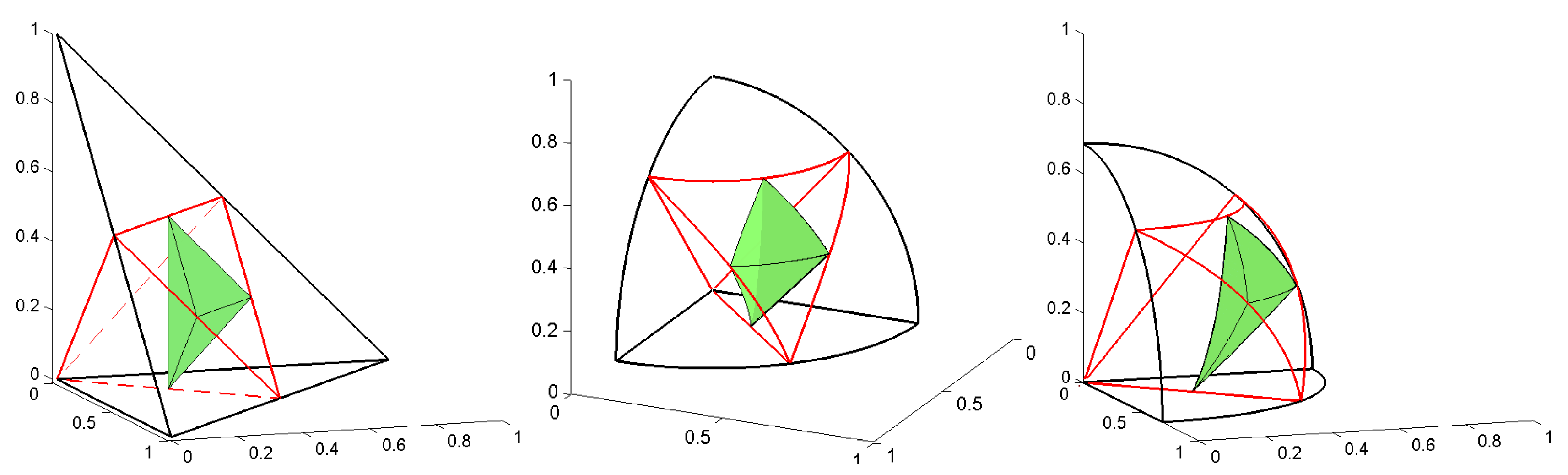
4.3. Uniform and Refinable Grids of the Ball ${\mathbb{B}}^3$

If we transport the uniform and refinable grid on $\mathbb{K}$ onto the ball ${\mathbb{B}}^3$ using the volume preserving map ${\mathcal{U}}^{-1}$, we obtain a uniform and refinable grid of ${\mathbb{B}}^3$. Figure 8, Figure 9 and Figure 10 show the images on ${\mathbb{B}}^3$ of different cells of $\mathbb{K}$.

Besides the multiresolution analysis and wavelet bases, which will be constructed in Section 5, another useful application is the construction of a uniform sampling of the rotation group $SO\left(3\right)$, by calculations similar to the ones in [3]. This will be subject of a future paper.

5. Multiresolution Analysis and Piecewise Constant Orthonormal Wavelet Bases of $L^2\left(\mathbb{K}\right)$ and $L^2\left({\mathbb{B}}^3\right)$

Let $\mathcal{D}={\mathcal{D}}^0=\{D_1,D_2,D_3,D_4\}$ be the decomposition of the domain $\mathbb{K}$ considered in Section 4.1, consisting in four congruent domains (cells) of type ${\mathbf{T}}_0$. For $D\in \mathcal{D},$ let ${\mathcal{R}}_D$ denote the set of the eight refined domains, constructed in Section 4.1.1. The set ${\mathcal{D}}^1={\cup }_{D\in {\mathcal{D}}^0}{\mathcal{R}}_D$ is a refinement of ${\mathcal{D}}^0$, consisting in $4·8$ congruent cells. Continuing the refinement process as we described in Section 4, we obtain a decomposition ${\mathcal{D}}^j$ of $\mathbb{K},$ for $j\in {\mathbb{N}}_0,$$\left|{\mathcal{D}}^j\right|=4·8^j$.

For a fixed $j\in {\mathbb{N}}_0$ we assign to each domain $D_k^j\in {\mathcal{D}}^j$, $k\in {\mathcal{N}}_j:={\mathbb{N}}_{4·8^j}$, the function ${\phi }_{D_k^j}:\mathbb{K}\to \mathbb{R},$

$${\phi }_{D_k^j}={\left(2\sqrt{2}\right)}^j\frac{2}{\sqrt{\mathrm{vol}\left(\mathbb{K}\right)}}{\chi }_{D_k^j},$$

where ${\chi }_{D_k^j}$ is the characteristic function of the domain $D_k^j$. Then we define the spaces of functions $V^j=\mathrm{span}\{{\phi }_{D_k^j},k\in {\mathcal{N}}_j\}$ of dimension $4·8^j$, consisting of piecewise constant functions on the domains of ${\mathcal{D}}^j.$ Moreover, we have $\parallel {\phi }_{D_k^j}{\parallel }_{L^2\left(\mathbb{K}\right)}=1$, the norm being the usual 2-norm of the space $L^2\left(\mathbb{K}\right)$. For $A^j\in {\mathcal{D}}^j=\{D_k^j,j\in {\mathcal{N}}_j\}$, let $A_k^{j+1},$ $k\in {\mathbb{N}}_8$, be the refined subdomains obtained from $A^j$. One has

$${\phi }_{A^j}=\frac{1}{2\sqrt{2}}({\phi }_{A_1^{j+1}}+{\phi }_{A_2^{j+1}}+\dots +{\phi }_{A_8^{j+1}}),$$

in $L^2\left(\mathbb{K}\right)$, equality which implies the inclusion $V^j\subseteq V^{j+1}$, for all $j\in {\mathbb{N}}_0$. With respect to the usual inner product ${\langle ·,·\rangle }_{L^2\left(\mathbb{K}\right)}$, the spaces $V^j$ are Hilbert spaces, with the corresponding usual 2-norm ${\parallel ·\parallel }_{L^2\left(\mathbb{K}\right)}$. In conclusion, the sequence of subspaces $V^j$ has the following properties:

• $V^j\subseteq V^{j+1}\mathrm{for}\mathrm{all}j\in {\mathbb{N}}_0$,
• ${\mathrm{clos}}_{L^2\left(\mathbb{K}\right)}{\bigcup }_{j=0}^{\infty }{V}^j=L^2\left(\mathbb{K}\right)$,
• The set $\{{\phi }_{D_k^j},k\in {\mathcal{N}}_j\}$ is an orthonormal basis of the space $V^j$ for each $j\in {\mathbb{N}}_0$,

i.e., the sequence $\{V^j,j\in {\mathbb{N}}_0\}$ constitutes a multiresolution analysis of the space $L^2\left(\mathbb{K}\right)$. Let $W^j$ denote the orthogonal complement of the coarse space $V^j$ in the fine space $V^{j+1},$ so that

$$V^{j+1}=V^j\oplus W^j.$$

The dimension of $W^j$ is $\dim W^j=28·8^j$. The spaces $W^j$ are called wavelet spaces and their elements are called wavelets. In the following we construct an orthonormal basis of $W^j$. To each domain $A^j\in {\mathcal{D}}^j$, seven wavelets supported on $D^j$ will be associated in the following way:

$${\psi }_{A^j}^{\ell }=a_{\ell 1}{\phi }_{A_1^{j+1}}+a_{\ell 2}{\phi }_{A_2^{j+1}}+\dots +a_{\ell 8}{\phi }_{A_8^{j+1}},\mathrm{for}\ell \in {\mathbb{N}}_7,$$

with $a_{\ell j}\in \mathbb{R},$ $\ell \in {\mathbb{N}}_7,$ $j\in {\mathbb{N}}_8.$ We have to find conditions on the coefficients $a_{\ell j}$ which ensure that the set $\{{\psi }_{A^j}^{\ell },\ell \in {\mathbb{N}}_7,A^j\in {\mathcal{D}}^j\}$ is an orthonormal basis of $W^j$. First we must have

$$\langle {\psi }_{A^j}^{\ell },{\phi }_{S^j}\rangle =0,\mathrm{for}\ell \in {\mathbb{N}}_7\mathrm{and}{A}^j,S^j\in {\mathcal{D}}^j.$$

(16)

If $A^j\ne S^j$, the equality is immediate, since $\mathrm{supp}{\psi }_{A^j}^{\ell }\subseteq \mathrm{supp}{\phi }_{A^j}$ and $\mathrm{supp}{\phi }_{A^j}\cap \mathrm{supp}{\phi }_{S^j}$ is either empty or an edge, whose measure is zero. If $A^j=S^j$, evaluating the inner product (16) we obtain

$$\begin{array}{ccc}\hfill \langle {\psi }_{A^j}^{\ell },{\phi }_{S^j}\rangle & =& \langle a_{\ell 1}{\phi }_{A_1^{j+1}}+a_{\ell 2}{\phi }_{A_2^{j+1}}+\dots +a_{\ell 8}{\phi }_{A_8^{j+1}},{\phi }_{A^j}\rangle \hfill \\ & =& \frac{1}{2\sqrt{2}}(a_{\ell 1}+a_{\ell 2}+\dots +a_{\ell 8}).\hfill \end{array}$$

Then, each of the orthogonality conditions

$$\langle {\psi }_{A^j}^{\ell },{\psi }_{A^j}^{\ell {}^{\prime }}\rangle ={\delta }_{\ell \ell {}^{\prime }},\mathrm{for}\mathrm{all}{A}^j\in {\mathcal{D}}^j,$$

is equivalent to $a_{\ell {}^{\prime }1}{a}_{\ell 1}+a_{\ell {}^{\prime }2}{a}_{\ell 2}+\dots +a_{\ell {}^{\prime }8}{a}_{\ell 8}={\delta }_{\ell \ell {}^{\prime }},$ $\ell ,{\ell }^{\prime }\in {\mathbb{N}}_7$. In fact, one requires the orthogonality of the $8\times 8$ matrix $M={\left(a_{ij}\right)}_{i,j}$ with the entries of the first row equal to $1/\left(2\sqrt{2}\right)$.

A particular case was considered in [12], where the authors divide a tetrahedron into eight small tetrahedrons of the same area using Bey’s method and for the construction of the orthonormal wavelet basis they take the Haar matrix

$$\frac{1}{2\sqrt{2}}\left(\begin{array}{cccccccc}1& 1& 1& 1& 1& 1& 1& 1\\ 1& 1& 1& 1& -1& -1& -1& -1\\ 1& 1& -1& -1& 0& 0& 0& 0\\ 0& 0& 0& 0& 1& 1& -1& -1\\ 1& -1& 0& 0& 0& 0& 0& 0\\ 0& 0& 1& -1& 0& 0& 0& 0\\ 0& 0& 0& 0& 1& -1& 0& 0\\ 0& 0& 0& 0& 0& 0& 1& -1\end{array}\right)$$

Alternatively, we can consider the symmetric orthogonal matrix

$$\left(\begin{array}{cccccccc}c& c& c& c& c& c& c& c\\ c& a& b& b& b& b& b& b\\ c& b& a& b& b& b& b& b\\ c& b& b& a& b& b& b& b\\ c& b& b& b& a& b& b& b\\ c& b& b& b& b& a& b& b\\ c& b& b& b& b& b& a& b\\ c& b& b& b& b& b& b& a\end{array}\right),$$

with

$$a=\frac{\pm 24-\sqrt{2}}{28},b=\frac{\mp 4-\sqrt{2}}{28},c=\frac{1}{2\sqrt{2}},$$

or the tensor product $H\otimes H\otimes H$ of the matrix

$$H=\frac{1}{\sqrt{2}}\left(\begin{array}{cc}1& 1\\ 1& -1\end{array}\right),\mathrm{which}\mathrm{is}$$

$$\begin{array}{c}\hfill \frac{1}{2\sqrt{2}}\left(\begin{array}{cccccccc}1& 1& 1& 1& 1& 1& 1& 1\\ 1& -1& 1& -1& 1& -1& 1& -1\\ 1& 1& -1& -1& 1& 1& -1& -1\\ 1& -1& -1& 1& 1& -1& -1& 1\\ 1& 1& 1& 1& -1& -1& -1& -1\\ 1& -1& 1& -1& -1& 1& -1& 1\\ 1& 1& -1& -1& -1& -1& 1& 1\\ 1& -1& -1& 1& -1& 1& 1& -1\end{array}\right)\end{array}$$

or, more general, we can generate all orthogonal $8\times 8$ matrices with the entries of the first row equal to $1/\left(2\sqrt{2}\right)$ using the method described in [13], where we start with the well known Euler’s formula for the general form of a $3\times 3$ rotation matrix. It is also possible to use different orthogonal matrices for the wavelets associated to the decomposition of the cells of type $\mathbf{T}$ and $\mathbf{M}$.

Next, following the ideas in [14] we show how one can transport the above multiresolution analysis and wavelet bases on the 3D ball ${\mathbb{B}}^3$, using the volume preserving map $\mathcal{U}:{\mathbb{B}}^3\to \mathbb{K}$ constructed in Section 3.

Consider the ball ${\mathbb{B}}^3$ is given by the parametric equations

$$\xi =\xi (X,Y,Z)={\mathcal{U}}^{-1}(X,Y,Z)=\left(x\right(X,Y,Z),y(X,Y,Z),z(X,Y,Z\left)\right),$$

with $(X,Y,Z)\in \mathbb{K}$. Since $\mathcal{U}$ and its inverse preserve the volume, the volume element $d\omega \left(\xi \right)$ of ${\mathbb{B}}^3$ equals the volume element $dXdYdZ=d\mathbf{x}$ of $\mathbb{K}$ (and ${\mathbb{R}}^3$). Therefore, for all $\tilde{f},\tilde{g}\in L^2\left({\mathbb{B}}^3\right)$ we have

$$\begin{array}{ccc}\hfill {\langle \tilde{f},\tilde{g}\rangle }_{L^2\left({\mathbb{B}}^3\right)}& =& {\int }_{{\mathbb{B}}^3}\overline{\tilde{f}\left(\xi \right)}\tilde{g}\left(\xi \right)d\omega \left(\xi \right)\hfill \\ & =& {\int }_{\mathcal{U}\left({\mathbb{B}}^3\right)}\overline{\tilde{f}\left({\mathcal{U}}^{-1}(X,Y,Z)\right)}\tilde{g}\left({\mathcal{U}}^{-1}(X,Y,Z)\right)dXdYdZ\hfill \\ & =& {\langle \tilde{f}\circ {\mathcal{U}}^{-1},\tilde{g}\circ {\mathcal{U}}^{-1}\rangle }_{L^2\left(\mathbb{K}\right),}\hfill \end{array}$$

and similarly, for all $f,g\in L^2\left(\mathbb{K}\right)$ we have

$${\langle f,g\rangle }_{L^2\left(\mathbb{K}\right)}={\langle f\circ \mathcal{U},g\circ \mathcal{U}\rangle }_{L^2\left({\mathbb{B}}^3\right)}.$$

(17)

If we consider the map $\mathsf{\Pi }:L^2\left({\mathbb{B}}^3\right)\to L^2\left(\mathbb{K}\right)$ induced by $\mathcal{U}$, defined by

$$\left(\mathsf{\Pi }\tilde{f}\right)(X,Y,Z)=\tilde{f}\left({\mathcal{U}}^{-1}(X,Y,Z)\right),\mathrm{for}\mathrm{all}\tilde{f}\in L^2\left({\mathbb{B}}^3\right),$$

and its inverse ${\mathsf{\Pi }}^{-1}:L^2\left(\mathbb{K}\right)\to L^2\left({\mathbb{B}}^3\right),$

$$\left({\mathsf{\Pi }}^{-1}f\right)\left(\xi \right)=f\left(\mathcal{U}\left(\xi \right)\right),\mathrm{for}\mathrm{all}f\in L^2\left(\mathbb{K}\right),$$

then $\mathsf{\Pi }$ is a unitary map, that is

$$\begin{array}{c}\hfill {\langle \mathsf{\Pi }\tilde{f},\mathsf{\Pi }\tilde{g}\rangle }_{L^2\left(\mathbb{K}\right)}={\langle \tilde{f},\tilde{g}\rangle }_{L^2\left({\mathbb{B}}^3\right)},\end{array}$$

(18)

$$\begin{array}{c}\hfill {\langle {\mathsf{\Pi }}^{-1}f,{\mathsf{\Pi }}^{-1}g\rangle }_{L^2\left({\mathbb{B}}^3\right)}={\langle f,g\rangle }_{L^2\left(\mathbb{K}\right)}.\end{array}$$

(19)

Equality (17) suggests us the construction of orthonormal scaling functions and wavelets defined on ${\mathbb{B}}^3$. The scaling functions $\widetilde{{\phi }_{D_k^j}}:{\mathbb{B}}^3\to \mathbb{R}$ will be

$$\widetilde{{\phi }_{D_k^j}}={\phi }_{D_k^j}\circ \mathcal{U}=\{\begin{array}{cc}1,& \mathrm{on}{\mathcal{U}}^{-1}\left(D_k^j\right),\hfill \\ 0,& \mathrm{in}\mathrm{rest}.\hfill \end{array}$$

(20)

and the wavelets will be defined similarly,

$$\widetilde{{\psi }_{A^j}^{\ell }}={\psi }_{A^j}^{\ell }\circ \mathcal{U}.$$

From equality (17) we can conclude that the spaces

$$\widetilde{V^j}:=\mathrm{span}\{\widetilde{{\phi }_{D_k^j}},k\in {\mathcal{N}}_j\}$$

constitute a multiresolution analysis of $L^2\left({\mathbb{B}}^3\right)$, each of the set $\{\widetilde{{\phi }_{D_k^j}},k\in {\mathcal{N}}_j\}$ being an orthonormal basis for the space $\widetilde{V^j}$. Moreover, the set

$$\{\widetilde{{\psi }_{A^j}^{\ell }},\ell \in {\mathbb{N}}_7,A^j\in {\mathcal{D}}_j\}$$

is an orthonormal basis of $\widetilde{W^j}$.

6. Conclusions and Future Works

The 3D uniform hierarchical grid constructed here can find applications in texture analysis of crystalls, by constructing a grid in the space of 3D rotations, using the technique used in [3]. A comparison of these grids is subject of a future paper.

Another interesting topic which we are going to approach in the future is to compare our wavelets with other 3D wavelets on the ball, listed in the introduction.

References

1. Moons, T.; van Gool, L.; Vergauwen, M. 3D reconstruction from multiple images part 1: Principles. Found. Trends Comput. Graph. Vis. 2010, 4, 287–404. [Google Scholar] [CrossRef]
2. Kendrew, J.C.; Bodo, G.; Dintzis, H.M.; Parrish, R.G.; Wyckoff, H.; Phillips, D.C. A Three-Dimensional Model of the Myoglobin Molecule Obtained by X-Ray Analysis. Nature 1958, 181, 662–666. [Google Scholar] [CrossRef] [PubMed]
3. Roşca, D.; Morawiec, A.; de Graef, M. A new method of constructing a grid in the space of 3D rotations and its applications to texture analysis. Model. Simul. Mater. Sci. Eng. 2014, 22, 075013. [Google Scholar] [CrossRef]
4. Flenger, M.; Michel, D.; Michel, V. Harmonic spline-wavelets on the 3D ball and their application to the reconstruction of the Earth’s density distribution from gravitational data and arbitrary shaped satellite orbits. ZAMM J. Appl. Math. Mech. 2006, 86, 856–873. [Google Scholar]
5. Simons, F.J.; Loris, I.; Nolet, G.; Daubechies, I.; Voronin, S.; Judd, J.S.; Vetter, P.A.; Charléty, J.; Vonesch, C. Solving or resolving global tomographic models with spherical wavelets, and the scale and sparsity of seismic heterogeneity. Geophys. J. Int. 2011, 187, 969–988. [Google Scholar] [CrossRef]
6. Simons, F.J.; Loris, I.; Brevdo, E.; Daubechies, I. Wavelets and wavelet-like transforms on the sphere and their application to geophysical data inversion. In Wavelets and Sparsity XIV; Papadakis, M., Van de Ville, D., Goyal, V.K., Eds.; International Society for Optics and Photonics: San Diego, CA, USA, 2011; Volume 81380, pp. 1–15. [Google Scholar]
7. Chow, A. Orthogonal and Symmetric Haar Wavelets on the Three-Dimensional Ball. Master’s Thesis, University of Toronto, Toronto, ON, Canada, 2010. [Google Scholar]
8. Leistedt, B.; McEwen, J.D. Exact wavelets on the ball. IEEE Trans. Signal Process. 2012, 60, 6257–6269. [Google Scholar] [CrossRef]
9. Loris, I.; Simons, F.J.; Daubechies, I.; Nolet, G.; Fornasier, M.; Vetter, P.; Judd, S.; Voronin, S.; Vonesch, C.; Charléty, J. A new approach to global seismic tomography based on regularization by sparsity in a novel 3D spherical wavelet basis. In Proceedings of the EGU General Assembly Conference Abstracts, ser. EGU General Assembly Conference Abstracts, Vienna, Austria, 2–7 May 2010; Volume 12, p. 6033. [Google Scholar]
10. Michel, V. Wavelets on the 3 dimensional ball. Proc. Appl. Math. Mech. 2005, 5, 775–776. [Google Scholar] [CrossRef]
11. Roşca, D. Locally supported rational spline wavelets on the sphere. Math. Comput. 2005, 74, 1803–1829. [Google Scholar] [CrossRef]
12. Boscardin, L.B.; Castro, L.R.; Castro, S.M. Haar-Like Wavelets over Tetrahedra. J. Comput. Sci. Technol. 2017, 17, 92–99. [Google Scholar] [CrossRef]
13. Pop, V.; Roşca, D. Generalized piecewise constant orthogonal wavelet bases on 2D-domains. Appl. Anal. 2011, 90, 715–723. [Google Scholar] [CrossRef]
14. Roşca, D. Wavelet analysis on some surfaces of revolution via area preserving projection. Appl. Comput. Harm. Anal. 2011, 30, 272–282. [Google Scholar] [CrossRef] [Green Version]
Figure 1. The eight spherical zones obtained as intersections of the coordinate planes with the ball B 3 .
Mathematics 08 00994 g001
Figure 2. The spherical region O A M C and its image O A M C = U ( O A M C ) on the octahedron.
Mathematics 08 00994 g002
Figure 3. Left: one of the four cells of type T 0 constituting the octahedron. Right: each cell of type T 0 can be subdivided into six cells of type T 1 and two cells of type M 1 .
Mathematics 08 00994 g003
Figure 4. The subdivision of a T cell.
Mathematics 08 00994 g004
Figure 5. The first step of the refinement: the cell T 0 is divided into two cells of type M 1 (yellow) and six cells of type T 1 : two red, two blue and two green.
Mathematics 08 00994 g005
Figure 6. The four cells of type T of the subdivision of a cell of type M .
Mathematics 08 00994 g006
Figure 7. The subdivision of a cell of type M 1 into four cells of type M : the four tetrahedrons at the corners and four cells of type T in the middle, forming an octahedron.
Mathematics 08 00994 g007
Figure 8. Left: a cell of M in red and a cell of T type in green from the octahedron Middle and right: the corresponding cells of the ball.
Mathematics 08 00994 g008
Figure 9. Left: the image on the ball of the positive octant; Right: the same image rotated.
Mathematics 08 00994 g009
Figure 10. The image on the ball of the cells of the octahedron corresponding to Figure 7.
Mathematics 08 00994 g010