Article

A Simple Method for Network Visualization

Department of Mathematics, Korea University, Seoul 02841, Korea
*
Author to whom correspondence should be addressed.
Mathematics 2020, 8(6), 1020; https://doi.org/10.3390/math8061020
Submission received: 16 May 2020 / Revised: 17 June 2020 / Accepted: 19 June 2020 / Published: 22 June 2020
(This article belongs to the Special Issue Numerical Methods)

Abstract

:
In this article, we present a simple method for network visualization. The proposed method is based on distmesh [P.O. Persson and G. Strang, A simple mesh generator in MATLAB, SIAM Review 46 (2004) pp. 329–345], which is a simple unstructured triangular mesh generator for geometries represented by a signed distance function. We demonstrate a good performance of the proposed algorithm through several network visualization examples.

1. Introduction

Since the formation of society, the relationships between its components have been significant. These relationships become more complex as society progresses; in addition, the components of society have also diversified. In sociology, a bundle of relationships is referred to as a network, which became a central concept in sociology in the 1970s. In a modern society called an information society, we have information regarding networks that has been transformed into concrete data. With a vast amount of information, information visualization has been used to analyze network and is gaining popularity. Techniques for information visualization have evolved, and they vary depending on the type of data [1,2,3,4]. Among the methods, visualization using graphs is one of the most helpful for understanding data and their relationships. The authors in [5] showed various graphs used in information visualization including tree layouts, H-tree layouts, balloon layout, radial layout, hyperbolic trees, fisheye graphs, and animated radial layouts (see Figure 1 as an example of network plot). Furthermore, toolkits for information visualization such as Prefuse, Protovis, and GUESS have been developed and widely used [1,6,7,8]. In several studies, nodes represent subjects, such as people and businesses, whereas edges represent relationships, such as friendships and partnerships. The scope of a network is not limited to people and institutions: if something is in an interactive relationship, we can call it a network, and networks can be also graphically identified by data. Network visualization is therefore being used in a variety of fields. For example, analysis for social and personal networks [9], pharmacological networks [10], biological networks [11,12], financial networks [13], and street networks [14] have been actively conducted.
Automatically drawing a network diagram requires algorithms. One of such algorithms is a classical force-directed algorithm that employs straight-edges. The force-directed algorithm treats edges as springs [16]. This algorithm turned the graph representation problem into a mathematical optimization problem. In other words, by reducing the energy generated by the spring system, we can find the equilibrium of the graph. The force-directed method has advantages such as simplicity to use and a good theoretical basis. As a result, many new methods of graph representation have been developed based on the method. As a typical example, Kamada and Kawai introduced an ideal distance for drawing graphs [17]. Let { X 1 , X 2 , , X n } be n-vertices and assume that they are spring-connected. The total energy of the spring is then expressed as follows:
E = i = 1 n 1 j = i + 1 n 2 ( | X i X j | l i j ) 2 ,
where l i j is the desirable length of the spring between X i and X j , k i j is a parameter representing the strength of this spring, and | · | is the Euclidean norm. The desirable length represents the final length after executing the algorithm, and the strength of the spring refers to the tension of the spring keeping certain distance. The best graph is determined by minimizing E . Please refer to [17] for more details about the algorithm and parameter definition. Another approach for automatically drawing a network diagram is based on the algorithm presented by Hall [18]. The main idea of this algorithm is to find the position of nodes { X 1 , X 2 , , X N } which minimizes
E = i < j N a i j | X i X j | 2 ,
where a i j 0 is the connection weight between X i and X j . This algorithm is suitable for application to a structured data such as polyhedron [19]. However, it may not work well on actual data [20]. Rücker and Schwarzer et al. [20] introduced a method of automatically drawing network diagrams using graph theory and studied network meta-analysis. Furthermore, the algorithm was applied to a variety of examples from the literature. Another representative method for drawing network diagrams is the stress majorization [21]. The objective function is defined as follows:
E = i j N w i j ( | X i X j | d i j ) 2 ,
where w i j is the weight between X i and X j , and d i j is an ideal distance. For additional details about the algorithm, please refer to [21]. This algorithm was applied to real networks related to diseases and implemented by using the function netgraph in the R package netmeta [20].
We propose a simple algorithm for network visualization based on the distmesh algorithm [22] in this paper. The proposed method employs a distance d i j , which is given by a reciprocal of weight w i j , hence the computing process is essentially simple. Furthermore, the position of nodes is renewed proportionally by the net force, which is based on the gradient, therefore one can obtain an optimal diagram to the given data. A two-step stopping criterion is applied to further maximize the visual effect of the network diagram. Compared to other methods based on the gradient to optimize total level of movements, for instance, the force-directed method, the stress majorization method, etc., our proposed algorithm is simple to implement.
The contents of this article are organized as follows. In Section 2, the proposed algorithm is described. In Section 3, specific examples of network visualization are presented. Conclusions are presented in Section 4.

2. Numerical Algorithm

2.1. Distmesh Algorithm
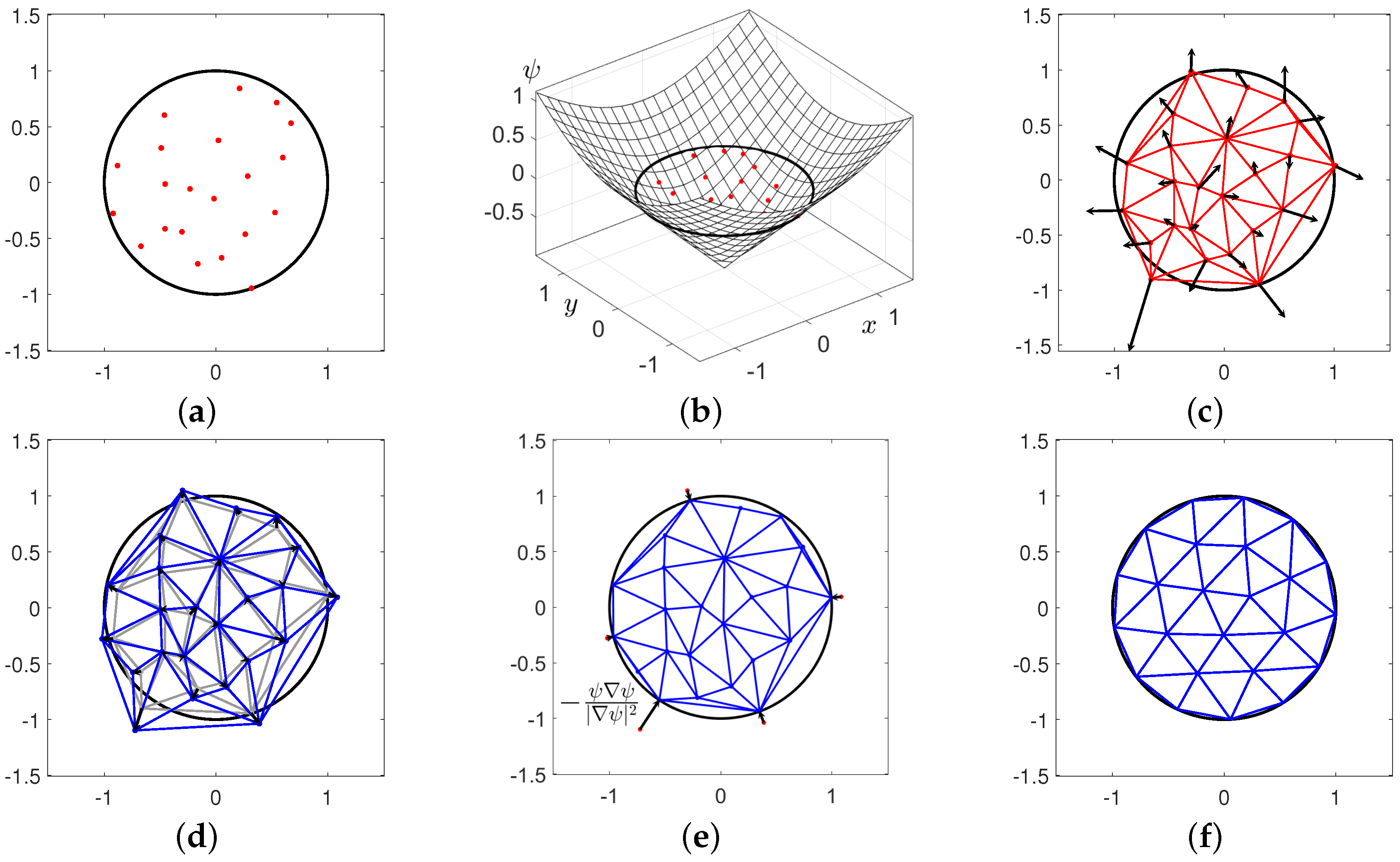
A brief introduction to the distmesh algorithm [22], which is employed to generate the triangular mesh in domain with the level set representation, is presented in this section. We define the level set representation in the two-dimensional domain which imposes that the interface structure is treated as the zero-level set. The following procedure depicts the whole algorithm of the distmesh. A function ψ ( x , y ) = x 2 + y 2 1 is adopted to a sample level set description. Figure 2 depicts the overall process of distmesh algorithm quite in detail.
Step 1. 
Generate the random nodes X 0 in domain.
Step 2. 
Generate a level set function ψ in the bounding box which includes the domain. The boundary of domain is regarded as the zero-level set.
Step 3. 
Perform the Delaunay triangulation with X n if the maximal arrangement of nodes is greater than certain level. If n = 0 , an initial Delaunay triangulation is accomplished. For the next step, compute the net force F in order to update the position of nodes.
Step 4. 
Renew the position of nodes to X n + 1 / 2 by adding Δ t F .
Step 5. 
Push back the nodes that are pushed out to the boundary into the interface using the following equation
X i n + 1 = χ ( X i n + 1 / 2 ) X i n + 1 / 2 ψ ( X i n + 1 / 2 ) | ψ ( X i n + 1 / 2 ) | 2 ψ ( X i n + 1 / 2 ) ,
where χ ( X i n + 1 / 2 ) is 1 if X i n + 1 / 2 is placed outside of the boundary; otherwise 0.
Step 6. 
Repeat Step 3–5 until the level of the total movement of nodes is less than a given tolerance.
Using the distmesh algorithm, triangular mesh generation can be performed nonuniformly on domain of various shapes. The following Figure 3 is an example of such generated mesh.

2.2. Proposed Algorithm for Network Visualization

The proposed algorithm for network visualization seeks to find { X 1 , X 2 , , X N } that minimize the objective function
E = i < j N w i j | | X i X j | d i j | 2 ,
where w i j and d i j are the weighting value and the desired distance between nodes X i and X j , respectively. The proposed algorithm is based on distmesh [22], which is a simple unstructured triangular mesh generator for geometries represented by a signed distance function. Let { X 1 n , X 2 n , , X N n } be given node positions at iteration n. For simplicity of exposition, we assume 0 w i j 1 . We then propose the following distance function:
d i j = d ( w i j ) = 1 w i j p , for w i j > 0 ,
where p is a constant. Let minW be the minimum positive value of w i j , i.e.,
minW = min 1 i , j N w i j > 0 w i j .
As shown in Figure 4, by setting the minimum distance minD = 1 when w i j = 1 and the maximum distance maxD when w i j = minW , we obtain
p = ln ( minD ) ln ( minW ) .
Figure 5a,b show repulsive and attractive forces at nodes X i n and X j n when | X i n X j n | < d i j and | X i n X j n | > d i j , respectively.
We loop over all the line segments connecting two nodes and compute the net force vector F i n at each node point X i n :
F i n = j = 1 , j i w i j > 0 N ( | X i n X j n | d i j ) X j n X i n | X j n X i n | .
Then, we update the position of the node points as
X i n + 1 = X i n + Δ t F i n , for 1 i N ,
where Δ t is an artificial time step. Upon updating the position of the node points, the network diagram is drawn automatically. The iterative algorithm has reached an equilibrium state if
1 N i = 1 N | F i k | 2 < t o l 1
after k iterations.
As a concrete example, we consider three points X 1 , X 2 , and X 3 . Assume that the weighting matrix between X i and X j is given as
W = 0 2 4 2 0 1 4 1 0 .
We scale the matrix W by dividing the elements by the maximum value among elements and redefine W as
W = 0 0.5 1 0.5 0 0.25 1 0.25 0 .
Let X 1 0 = ( 1 4 , 3 3 4 ) , X 2 0 = ( 0 , 0 ) , and X 3 0 = ( 3 2 , 0 ) , where the superscript 0 denotes the starting index. Here, we use Δ t = 0.3 , minD = 1 , maxD = 2 , minW = 0.25 , and t o l 1 = 0.01 . Consequently, we get p = 0.5 and
d 12 d 13 d 21 d 23 d 31 d 32 = 2 1 2 2 1 2 .
Figure 6a indicates the position of the three points with red markers, and the non-zero elements of W are represented by gray lines. In particular, the values of each element is expressed by the thickness of the line. The red arrows are net force vectors F 1 0 , F 2 0 and F 3 0 . Using these net force vectors, we update the positions as
X 1 1 = X 1 0 + Δ t F 1 0 , X 2 1 = X 2 0 + Δ t F 2 0 , X 3 1 = X 3 0 + Δ t F 3 0 ,
which are shown in Figure 6b. Figure 6c–e show the network diagrams after 2, 3, and 6 iterations, respectively. The equilibrium state of the network diagram is obtained after 10 iterations as shown in Figure 6f. Even though the nodes are initially arranged in an equilateral triangle with sides of length 1.5, the network diagram in equilibrium is drawn according to the given weights.

3. Numerical Results

In this section, we present the generation of a network diagram with more data to confirm the efficiency and robustness of the proposed method. Specifically, we select 19 nodes and 19 × 19 matrix W , which are given in Appendix A. The matrix is created based on the dialogue between the characters in William Shakespeare’s play, ‘The Venice Merchant’. Each element w i j of the matrix is the cumulative number of conversations between person i and person j. The parameters used are Δ t = 0.01 , minD = 1 , maxD = 2 , and t o l 1 = 0.01 . The value of p is then approximately 0.1879 . Figure 7 shows process of the network visualization by our proposed method. The equilibrium state of the network diagram appears after 1985 iterations.
After 1985 iterations, each node is appropriately located according to the weights between the nodes in the network. This means that even if the nodes are initially randomly arranged, the network diagram is well drawn by our distance function. While the network plot is drawn, we can see that the objective function E is decreasing. As shown in Figure 8, E decreases and converges as time goes by. This shows that our proposed method has a mathematical basis for drawing the network diagram.
However, the equilibrium state network diagram is not visually good. This is due to the nodes (9, 13, 15, 16, 17, 18) that have only one connection. Therefore, we further update the location of the nodes that have only one connection while fixing the other nodes. Let Ω s be the index set of the nodes having only one connection. We compute the net force vector F i n at each node point i Ω s as follows:
F i n = j = 1 , j i w i j > 0 N X i n X j n | X i n X j n | .
Then, we temporally update the node points as
X i * = X i n + Δ t F i n for i Ω s ,
where Δ t = 10 is used. Finally, we set
X i n + 1 = X j n + d i j X i * X j n | X i * X j n | for i Ω s and X i n + 1 = X i n for i Ω s ,
where X j n is the unique node connecting X i * . We define that the equilibrium state of the second step has been attained if
1 | Ω s | i Ω s | X i k + 1 X i k | 2 < t o l 2
after k iterations, where | Ω s | is the counting measure. Here, t o l 2 = 0.002 is used. Therefore, the second step effectively rotates the node that has only one connection around the connecting node so that the overall distribution of the nodes is scattered.
Figure 9 illustrates the process of updating the position of nodes (red makers) that have only one connection. Figure 9a–d shows the network in the equilibrium state of the first step, after 1 iteration of the second step, after 2 iterations of the second step, and in the equilibrium state of the second step after 75 iterations.
Next, we consider another example ‘Romeo and Juliet’ which is a play written by William Shakespeare. Matrix W is defined by counting the number of conversations between 27 characters. The parameters used are minD = 1 , maxD = 3 , and t o l 1 = t o l 2 = 0.002 , and then the value of p is approximately 0.2493. In particular, time step Δ t = 0.2 and Δ t = 10 are used in the first step and the second step, respectively. Figure 10a–c illustrate the character network at the initial condition, after the first step, and after the second step, respectively. From the results, we can find the main characters and relatively small parts.

4. Conclusions

In this paper, we have proposed a simple method based on distmesh for network visualization. We have demonstrated the good performance of the proposed algorithm through network visualization examples. We can provide the MATLAB source code of this method for the interested readers. In future work, we plan to investigate effective network diagrams for character networks from novels and movies. We may further speed up the computation of the proposed method by using a Gauss–Newton–secant type method [23].

Author Contributions

All authors contributed equally to this work; J.P., S.Y., C.L. and J.K. critically reviewed the manuscript. All authors have read and agree to the published version of the manuscript.

Funding

The corresponding author (J. Kim) expresses thanks for the support from the BK21 PLUS program.

Acknowledgments

The authors thank the editor and the reviewers for their constructive and helpful comments on the revision of this article.

Conflicts of Interest

The authors declare no conflict of interest.

Appendix A

In this appendix, we provide the MATLAB source codes for network visualization. The following code is for ‘The Merchant of Venice’. The code for ‘Romeo and Juliet’ is available on the following website:
Listing A1. Matlab Code for the network visualization.
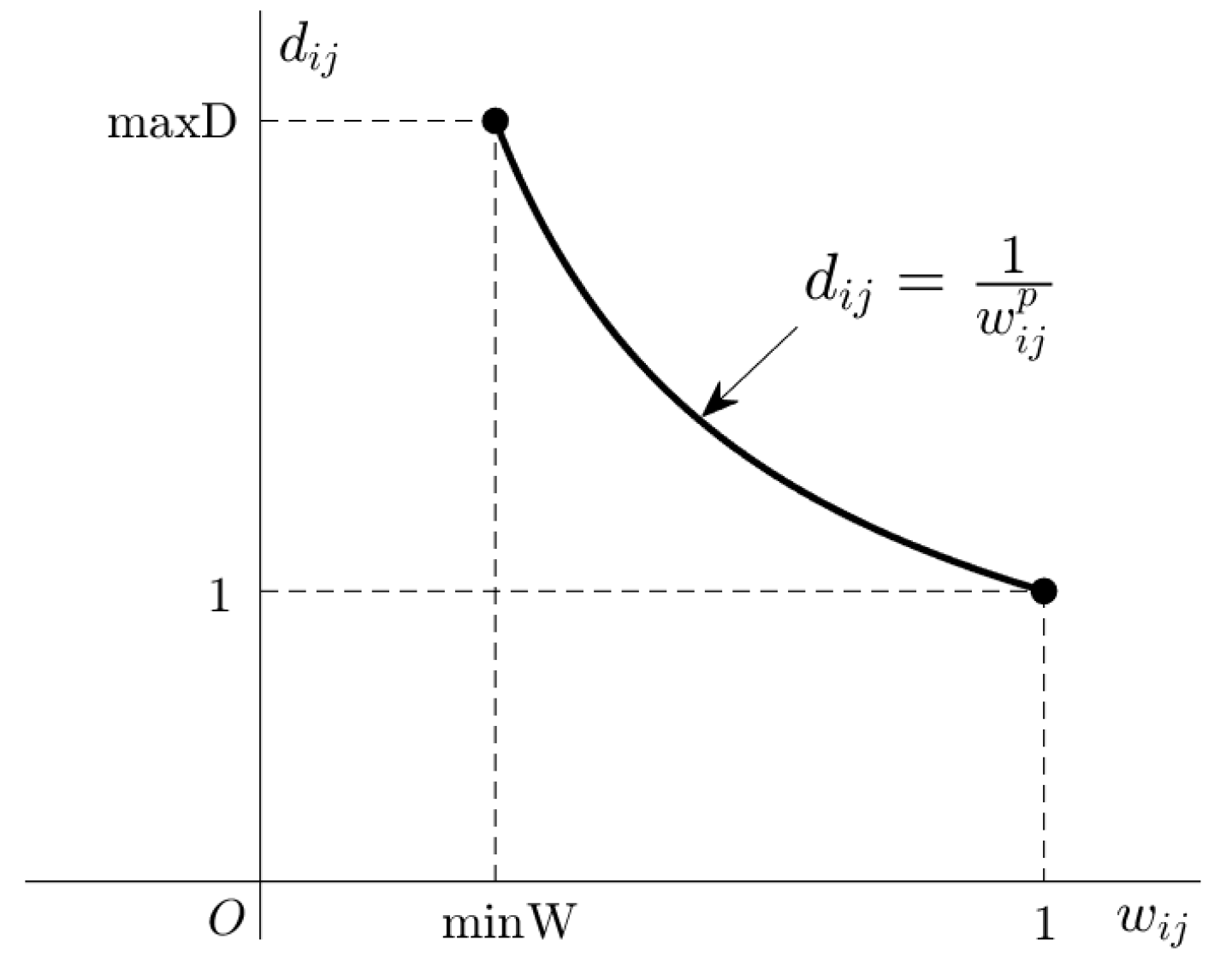
% The first step 
clear;
W=[ 0 21 24 16  0  0  0 2  0 7 4  5 0 0 0 0  0 0 1
   21  0 27 32  0  0  0 0  0 2 0 11 2 3 2 0  0 0 0
   24 27  0 40  0  0  7 0 12 6 0  2 0 5 0 0  0 0 2
   16 32 40  0 36  3  0 7  0 0 0 10 0 0 0 3 13 2 0
    0  0  0 36  0  2  0 0  0 0 0  4 0 0 0 0  0 0 0
    0  0  0  3  2  0 15 0  0 0 0  4 0 0 0 0  0 0 0
    0  0  7  0  0 15  0 0  0 0 0  0 0 3 0 0  0 0 0
    2  0  0  7  0  0  0 0  0 0 0  0 0 0 0 0  0 0 0
    0  0 12  0  0  0  0 0  0 0 0  0 0 0 0 0  0 0 0
    7  2  6  0  0  0  0 0  0 0 9  0 0 0 0 0  0 0 0
    4  0  0  0  0  0  0 0  0 9 0  0 0 0 0 0  0 0 0
    5 11  2 10  4  4  0 0  0 0 0  0 0 0 0 0  0 0 0
    0  2  0  0  0  0  0 0  0 0 0  0 0 0 0 0  0 0 0
    0  3  5  0  0  0  3 0  0 0 0  0 0 0 0 0  0 0 0
    0  2  0  0  0  0  0 0  0 0 0  0 0 0 0 0  0 0 0
    0  0  0  3  0  0  0 0  0 0 0  0 0 0 0 0  0 0 0
    0  0  0 13  0  0  0 0  0 0 0  0 0 0 0 0  0 0 0
    0  0  0  2  0  0  0 0  0 0 0  0 0 0 0 0  0 0 0
    1  0  2  0  0  0  0 0  0 0 0  0 0 0 0 0  0 0 0];
N=size(W,1); rand("seed",3773); t=rand(N,1);
xy=[cos(2*pi*t),sin(2*pi*t)]; W=W/max(max(W));
minW=min(min(W(W>0))); minD=1; maxD=2; p=-log(maxD)/log(minW);
for i=1:N
    for j=1:N
        if W(i,j)>0
         d(i,j)=1/W(i,j)^p;
        end
    end
end
dt=0.01; tol=0.01; n=0; error=2*tol;
while error≥tol
  n=n+1; F = zeros(N,2);
  for i=1:N
      for j=i+1:N
          if W(i,j)>0
            vt = xy(j,:)-xy(i,:);
            F(i,:) = F(i,:) + (norm(vt)-d(i,j))*vt/norm(vt);
            F(j,:) = F(j,:) − (norm(vt)-d(i,j))*vt/norm(vt);
         end
      end
  end
  xy = xy + dt*F; error=norm(F)/sqrt(N);
  if n==1 || mod(n,10)==0 || error<tol
     figure(1); DrawNetwork(xy,W); pause(0.1)
  end
end 
% The second step
z=find(sum(W>0)==1); M=length(z);
for k=1:M
    s(k)=find(W(z(k),:)>0);
end
xy0=xy; n=0; dt=10.0; tol=0.002; error=2*tol;
while error≥=tol
  n=n+1; F = zeros(N,2);
  for k=1:M
    v=[0 0];
        for j=1:N
            vt = xy(z(k),:)-xy(j,:);
            if norm(vt)>0
              v=v+vt/norm(vt);
            end
        end
    F(z(k),:)=v/norm(v);
  end
  xy = xy + dt*F;
  error=0;
  for k=1:M
      v=xy(z(k),:)-xy(s(k),:);
      xy(z(k),:)=xy(s(k),:)+d(z(k),s(k))*v/norm(v);
      error=error+norm(xy(z(k),:)-xy0(z(k),:))^2;
  end 
  error=sqrt(error/M); xy0=xy;
  figure(2); DrawNetwork(xy,W); pause(0.1)
end
Listing A2. Function code for DrawNetwork.
function DrawNetwork(xy,W)
N=length(xy); clf; hold on
for i=1:N
    for j=i+1:N
        if W(i,j)>0
        plot(xy([i,j],1),xy([i,j],2),"b","linewidth",15*W(i,j)^2+1);
        end
    end
end
scatter(xy(:,1),xy(:,2),400,"g","filled");
for i = 1:N
    text(xy(i,1)-0.04,xy(i,2),num2str(i));
end
axis off; axis image;
end

References

  1. Heer, J.; Card, S.K.; Landay, J.A. Prefuse: A toolkit for interactive information visualization. In Proceedings of the SIGCHI Conference on Human Factors in Computing Systems, Portland, OR, USA, 2–7 April 2005; pp. 421–430. [Google Scholar]
  2. Keim, D.A. Information visualization and visual data mining. IEEE Trans. Vis. Comput. Graph. 2002, 8, 1–8. [Google Scholar] [CrossRef]
  3. McGuffin, M.J. Simple algorithms for network visualization: A tutorial. Tsinghua Sci. Technol. 2012, 17, 383–398. [Google Scholar] [CrossRef]
  4. Van Wijk, J.J.; Van de Wetering, H. Cushion treemaps: Visualization of hierarchical information. In Proceedings of the 1999 IEEE Symposium on Information Visualization (InfoVis’ 99), San Francisco, CA, USA, 24–29 October 1999; pp. 73–78. [Google Scholar]
  5. Herman, I.; Melançon, G.; Marshall, M.S. Graph visualization and navigation in information visualization: A survey. IEEE Trans. Vis. Comput. Graph. 2000, 6, 24–43. [Google Scholar] [CrossRef] [Green Version]
  6. Adar, E. GUESS: A language and interface for graph exploration. In Proceedings of the SIGCHI Conference on Human Factors in Computing Systems, Montréal, QC, Cananda, 22–27 April 2006; pp. 791–800. [Google Scholar]
  7. Bostock, M.; Heer, J. Protovis: A graphical toolkit for visualization. IEEE Trans. Vis. Comput. Graph. 2009, 15, 1121–1128. [Google Scholar] [CrossRef] [PubMed]
  8. Wylie, B.; Baumes, J. A unified toolkit for information and scientific visualization. In Visualization and Data Analysis 2009; SPIE: San Jose, CA, USA, 2009; p. 72430H. [Google Scholar]
  9. McCarty, C.; Molina, J.L.; Aguilar, C.; Rota, L. A comparison of social network mapping and personal network visualization. Field Methods 2007, 19, 145–162. [Google Scholar] [CrossRef] [Green Version]
  10. Nüesch, E.; Häuser, W.; Bernardy, K.; Barth, J.; Jüni, P. Comparative efficacy of pharmacological and non-pharmacological interventions in fibromyalgia syndrome: Network meta-analysis. Ann. Rheum. Dis. 2013, 72, 955–962. [Google Scholar] [CrossRef] [PubMed]
  11. Wu, L.; Li, M.; Wang, J.X.; Wu, F.X. Controllability and Its Applications to Biological Networks. J. Comput. Sci. Technol. 2019, 34, 16–34. [Google Scholar] [CrossRef]
  12. Xia, M.; Wang, J.; He, Y. BrainNet Viewer: A network visualization tool for human brain connectomics. PLoS ONE 2013, 8, e68910. [Google Scholar] [CrossRef] [PubMed] [Green Version]
  13. Dolfin, M.; Knopoff, D.; Limosani, M.; Xibilia, M.G. Credit Risk Contagion and Systemic Risk on Networks. Mathematics 2019, 7, 713. [Google Scholar] [CrossRef] [Green Version]
  14. Pueyo, O.; Pueyo, X.; Patow, G. An overview of generalization techniques for street networks. Graph. Models 2019, 106, 101049. [Google Scholar] [CrossRef]
  15. Chaimani, A.; Higgins, J.P.; Mavridis, D.; Spyridonos, P.; Salanti, G. Graphical tools for network meta-analysis in STATA. PLoS ONE 2013, 8, e76654. [Google Scholar] [CrossRef] [PubMed]
  16. Eades, P. A heuristic for graph drawing. Congr. Numer. 1984, 42, 149–160. [Google Scholar]
  17. Kamada, T.; Kawai, S. An algorithm for drawing general undirected graphs. Inf. Process. Lett. 1989, 31, 7–15. [Google Scholar] [CrossRef]
  18. Hall, K.M. An r-dimensional quadratic placement algorithm. Manag. Sci. 1970, 17, 219–229. [Google Scholar] [CrossRef]
  19. Spielman, D. Spectral Graph Theory. In Combinatorial Scientific Computing (No. 18); CRC Press: Boca Raton, FL, USA, 2012. [Google Scholar]
  20. Rücker, G.; Schwarzer, G. Automated drawing of network plots in network meta-analysis. Res. Synth. Methods 2016, 7, 94–107. [Google Scholar] [CrossRef] [PubMed]
  21. Gansner, E.R.; Koren, Y.; North, S. Graph drawing by stress majorization. In International Symposium on Graph Drawing; Springer: Berlin/Heidelberg, Germany, 2004; pp. 239–250. [Google Scholar]
  22. Persson, P.O.; Strang, G. A simple mesh generator in MATLAB. SIAM Rev. Soc. Ind. Appl. Math. 2004, 46, 329–345. [Google Scholar] [CrossRef] [Green Version]
  23. Argyros, I.; Shakhno, S.; Shunkin, Y. Improved Convergence Analysis of Gauss-Newton-Secant Method for Solving Nonlinear Least Squares Problems. Mathematics 2019, 7, 99. [Google Scholar] [CrossRef] [Green Version]
Figure 1. Example of a circular network. Reprinted from Salanti et al. [15] with permission from PLoS ONE.
Mathematics 08 01020 g001
Figure 2. Schematic illustration of generating the distmesh. (a) Generated random nodes in the domain. (b) Signed distance function ψ in bounding box. The boundary of domain is regarded as the zero-level set. (c) Net force F in current triangulation. (d) Arrangement of nodes via Δ t F . (e) Projection of the nodes located outside ψ > 0 into the boundary ψ 0 using Equation (3). (f) Final result of unstructured mesh by using the distmesh algorithm.
Mathematics 08 01020 g002
Figure 3. Example of nonuniformly generated mesh: the airfoil.
Mathematics 08 01020 g003
Figure 4. Illustration of distance function d i j related to weighting value w i j . minD = 1 and maxD are set to appear when w i j = 1 and w i j = minW , respectively.
Mathematics 08 01020 g004
Figure 5. Two possible forces at nodes X i n and X j n : (a) repulsive force and (b) attractive force.
Mathematics 08 01020 g005
Figure 6. Schematic of the proposed algorithm. (a) initial condition, (b) after 1 iteration, (c) after 2 iterations, (d) after 3 iterations, (e) after 6 iterations, and (f) equilibrium state after 10 iterations.
Mathematics 08 01020 g006
Figure 7. Snapshots of the network visualization process for ‘The Venice Merchant’: (a) initial condition, (b) after 20 iteration, (c) after 40 iterations, and (d) equilibrium state after 1985 iterations.
Mathematics 08 01020 g007
Figure 8. E decreases and converges while each node is moving.
Mathematics 08 01020 g008
Figure 9. Updating the position of nodes with only one connection: (a) Equilibrium state of the first step, (b) after 1 iteration, (c) after 2 iterations, and (d) equilibrium state of the second step after 75 iterations.
Mathematics 08 01020 g009
Figure 10. Snapshots of network visualization for ‘Romeo and Juliet’: (a) the initial condition, (b) after 230 iterations of the first step, and (c) after 20 iterations of the second step.
Mathematics 08 01020 g010

