Article

Multi-Stack Lifetime Improvement through Adapted Power Electronic Architecture in a Fuel Cell Hybrid System

1
University of Lorraine, CNRS, LEMTA, 54000 Nancy, France
2
Renewable Energies Engineering Department, Shahid Beheshti University, Tehran 1983969411, Iran
*
Author to whom correspondence should be addressed.
Mathematics 2020, 8(5), 739; https://doi.org/10.3390/math8050739
Submission received: 31 March 2020 / Revised: 30 April 2020 / Accepted: 2 May 2020 / Published: 7 May 2020

Abstract

:
To deal with the intermittency of renewable energy resources, hydrogen as an energy carrier is a good solution. The Polymer Electrolyte Membrane Fuel Cell (PEMFC) as a device that can directly convert hydrogen energy to electricity is an important part of this solution. However, durability and cost are two hurdles that must be overcome to enable the mass deployment of the technology. In this paper, a management system is proposed for the fuel cells that can cope with the durability issue by a suitable distribution of electrical power between cell groups. The proposed power electronics architecture is studied in this paper. A dynamical average model is developed for the proposed system. The validation of the model is verified by simulation and experimental results. Then, this model is used to prove the stability and robustness of the control method. Finally, the energy management system is assessed experimentally in three different conditions. The experimental results validate the effectiveness of the proposed topology for developing a management system with which the instability of cells can be confronted. The experimental results verify that the system can supply the load profile even during the degradation mode of one stack and while trying to cure it.

1. Introduction

Based on the energy and environmental crisis in the world, the approach is toward using renewable and clean energy [1]. The most important issue of renewable energies is the intermittency of the resources [2,3,4]. Hydrogen as an energy carrier can cope with this problem [5]. This gas can be directly converted to electricity by a Polymer Electrolyte Membrane Fuel Cell (PEMFC) [4,6]. The nominal voltage of one cell is near 0.7 V. Therefore, a number of cells are connected in series inside of one stack to increase the output voltage. The basic disadvantage of such connections is the lifetime dependency of the stack on each cell lifetime. The other disadvantage of this connection is the probability of the fault propagation from one cell to the adjacent ones because of thermal coupling. The cell management can cope with these problems.
Currently, the performance of PEMFC, in terms of power density (3.1 kW/L) and electrical energy efficiency, is sufficient to allow large-scale deployment of the technology [7,8]. On the other hand, lifetime and cost are two points that need to be improved [9]. To improve the durability, it is possible to develop new materials more resistant but also to better manage the operating conditions to avoid the electrochemical instabilities that lead to irreversible damages [10]. For instance, a novel converter was proposed in [11] to reduce the current ripple for fuel cell applications. A specific management system like the battery management systems can deal with the instabilities of the cells inside a stack. For instance, if one cell is more degraded than other cells, its voltage decreases and it dissipates more heat. The direct consequence of the higher temperature of the degraded cell is the drying of its membrane and the subsequent increase of its ionic resistance that at the end amplifies the voltage loss. This snowball effect can destroy the cell. If it was possible to separately change the current of the damaged cells to produce more water or to reduce the heat production, it would deal with the mentioned snowball effect.
Developing such a management system for a single stack needs a special stack, which allows modifying the current of any number of cells inside the stack, and a power electronic structure that allows controlling the power flow of different cells. A new patent obviates the first requirement and allows access to the current of any cells [12]. Multi-stack can be considered as an attempt to increase the lifetime and durability of the fuel cell system at the cost of compactness loss. The multi-stack can be used for high power [13,14,15], vehicular and transportation [16,17,18,19,20,21,22,23,24], and stationary [16,25,26,27] applications due to its higher reliability and efficiency and its optimized fuel consumption. This technology has been already used by a Mercedes bus, power supplies of space exploration vehicles, and air-independent propulsion for submarines [28]. In [21], the multi-stack was investigated in the fault mode and the faulty stack could partially or totally be disconnected by a diode by-pass circuit while the other stacks supply the load. A model was also developed for the proposed architecture. Two PEMFC stacks with the rated power of 20 kW (total rated power of 40 kW) were used in [22] to totally supply a manned aircraft. Ten PEMFC stacks with the rated power of 480 kW were used in [27] to develop a stationary distributed generation system. In [23], a hybrid system of two PEMFC stacks with the rated power of 150 kW (total 300 kW) and a battery bank were used to supply a locomotive. The battery bank was used to supply the load profile over transient conditions.
As seen in Figure 1., four basic topologies are used for the multi-stack or segmented FCs: series, parallel, cascade, series-parallel [21,28]. The series topology (Figure 1a) requires a low voltage ratio converter. In such a connection, the failure of a single cell means losing the whole system. Furthermore, there is no freedom degree in controlling the cells separately. The second topology, which the cells or stacks separately connect to the DC link by individual converters, provides the freedom degree in controlling the cells [18]. However, the high conversion ratio converters, which are required to increase the output voltage, provide higher stress on the semiconductor devices. This architecture is the most expensive topology due to a great requirement of the passive energy storage components. The cascade topology resolves the problem of the parallel topology. In this topology, the DC-link voltage is divided between the cells. This leads to lower stress on semiconductor devices. The series-parallel topology (Figure 1d) is identical to the parallel topology except that more cells are connected to the input of each converter. This topology inherits the advantages and disadvantages of series and parallel topologies. In such a topology, the converters with lower voltage ratio can be used.
Considering the ability of separately controlling the cells or stacks, the cascade topology (Figure 1c) can be used to manage the cells. However, connecting the cells to the high voltage DC link while maintaining the controllability of each converter is challenging. It should be noted that the proposed structure can be used for a single stack that allows accessing the current of different cell groups or a multi-stack. As a result, the word stack is used instead of cell groups for the sake of simplicity in the rest of this paper.
Due to the low voltage of a cell or a small group of cells, a converter with a high voltage ratio has to be used [29,30]. In this paper, the classical DC–DC boost converters are used while their output capacitors are connected in series, inspired by the cascade topology. In such a connection, the same load current passes through all output capacitors. Therefore, if the input power of one cell becomes lower than the required amount, the voltage of the corresponding capacitor will decrease. In this case, the controllability will be lost if the output voltage becomes lower than the input voltage. As mentioned before, the objective is to develop a management system that separately controls the current of cells or stacks. Considering the cascade topology with N groups (Figure 2), if the load power (Pload) is constant and the DC-link voltage is regulated at Vdc, then the load current has a constant value of iload in steady-state and, as a result, the supplied power by cells can be calculated as P k = i l o a d V C k     k 1 , 2 , N . Assuming that the total supplied power by stacks is equal to the load power, and the first group of cells should inject a part (x) of the nominal power (Pload/N), whereas the other groups inject an identic value of power, the following equation can be obtained in steady-state as follows:
P 1 = x P l o a d N = i l o a d V C 1 V C 1 = x N V d c P k = N x N N 1 P l o a d = i l o a d V C k V C k = N x N N 1 V d c
where k in this equation can be 2 , 3 , N . The voltage of the first capacitor must be greater than the input voltage of the corresponding converter. Thus, considering the voltage ratio of the boost converter (Rv) and (1), x > N V F C V d c > 1 R v . Therefore, the supplied power of the first group cannot be less than 1 R v N P l o a d . Otherwise, the controllability is lost. In such conditions, a voltage equalizer or a balancing system has to be added to ensure the controllability of converters.
A new voltage equalizer, which was proposed in [31], is modified and used in this paper. In [32], the equalizer was controlled according to the voltage difference and a hysteresis method. The proportional gain controller, as used in [31], is improved in this paper to enhance the dynamical behavior of the equalization. The improved method can cope with the overvoltage of the output capacitors due to operating conditions of the fuel cell management system in some particular cases.
Due to dynamic constraints, the hybridization of a fuel cell with an energy storage system is required to supply a given load, especially for transport or stationary applications [23,33,34,35,36]. The battery has a high energy density and a higher power density than the FC. Therefore, the FC/Battery hybridization has been used in some papers [34,37,38,39]. Contrary to the batteries, supercapacitors (SCs) have a higher power density and a lower energy density than the batteries. As a result, the FC/SC hybrid system has been widely used in the literature due to the ability of the SC in compensating for the slow dynamic of the FC [34,40]. In [35,41,42], an FC/SC/Battery structure was proposed for vehicular application and an energy management strategy was proposed to supply the load. The main objective in [38,41,42] was to develop an energy management strategy to improve fuel consumption. In this paper, the main objective is to develop a system in which energy management can be implemented while curing the defective stacks.
The conventional hybridizing fuel cell with SC is used in this paper to respond to the high dynamic load profile. To regulate the output DC bus voltage, the SC is connected to the DC link through a bidirectional DC–DC boost converter.
The hybridized system with the equalizer system needs a control method that can be implemented easily and ensure the stability of the system. In this paper, a control method is proposed for the whole system.
An accurate model of the system has to be realized to perform the sizing of the passive elements and control parameters or/and dynamical stability analysis. There are three basic approaches to investigate the dynamic behavior of the system: Discrete-time model, Switching model, and Average model. In [43], these three approaches were used to investigate the dynamic behavior of a boost converter with a sliding mode current controller. In [44], the stability of a boost converter based on the discrete-time model and the average model was investigated when a hysteresis current controller was used. The dynamic behavior of a boost converter with an LC filter was investigated based on the discrete-time model approach in [45]. In [45], the output voltage and current of the boost converter were controlled based on the dynamic separation. The discrete-time model cannot be used especially for some complicated systems. For such systems, the average model can be used to study the dynamic behavior of the system. In [46], an interleaved-boost full-bridge converter was modeled by obtaining the state-space average models of the system over different operation modes. This kind of modeling approach can involve many equations for complex systems. Therefore, this model can be very complex. In [47], an average model was proposed to perform the stability analysis for a hybrid photovoltaic and wave power generation system. The average model of each system and control method were used to obtain an overall dynamic average model for the hybrid system. Then, the stability analysis, based on the eigenvalues of the proposed average state-space model, has been used to verify the stable operation of the system under various operating conditions. An average model based on the state-space equations of the system was introduced for a balancer in [48]. This balancer can equalize the voltage between two SC banks. Indeed, the proposed balancer was a synchronous buck-boost topology that can transfer the stored energy in the inductor of the converter to the banks and vice versa. In such a connection, there is no intermediary AC power stage. For systems with AC power stage, the average values of pure AC variables are equal to zero. This last property involves an order reduction to establish the average model. To deal with this phenomenon, the DC terms and the first-order terms of Fourier series of state variables were used in [49]. Since the transformer current of a dual active bridge converter is purely AC, its DC component is equal to zero. Therefore, the switching frequency terms in the Fourier series of state variables were used to capture the effect of the transformer current on the system dynamics in [49]. In [50], a dynamical average model was proposed for an isolated boost converter. In this converter, the average value of the transformer current over each period of switching is equal to zero. Therefore, the energy cannot be transferred through the transformer by using this average value in the average state-space model. The equation of the average value of the leakage current was obtained over a half period. Since the leakage current of the isolated boost converter is symmetric, this equation is valid for any half periods. As a result, the obtained average value is not equal to zero and the energy can be transferred through the transformer even in the average model. The main disadvantage of this approach is the assumption in which the transformer current waveform must be symmetrical.
In this paper, the proposed equalizer includes an AC power stage but the current waveforms can be asymmetrical. Thus, a reduced-order average model is proposed in which the symmetrical waveform of the transformer current is not mandatory. Moreover, the proposed average model takes into account the cross-coupling effect due to the serial connection of output capacitors. Dynamic stability analysis of the system is also performed based on the proposed model. This proposed approach is validated by simulation and experimental results.
The rest of this paper is organized as follows: The proposed system configuration, the improved control method, and the definition of the dynamical average model for any operating conditions are detailed in Section 2. The SC and DC-link voltage control methods are described in Section 3. The simulation and experimental results are presented in Section 4. The stability analysis and energy management are performed in Section 5. Finally, conclusions are presented in Section 6.

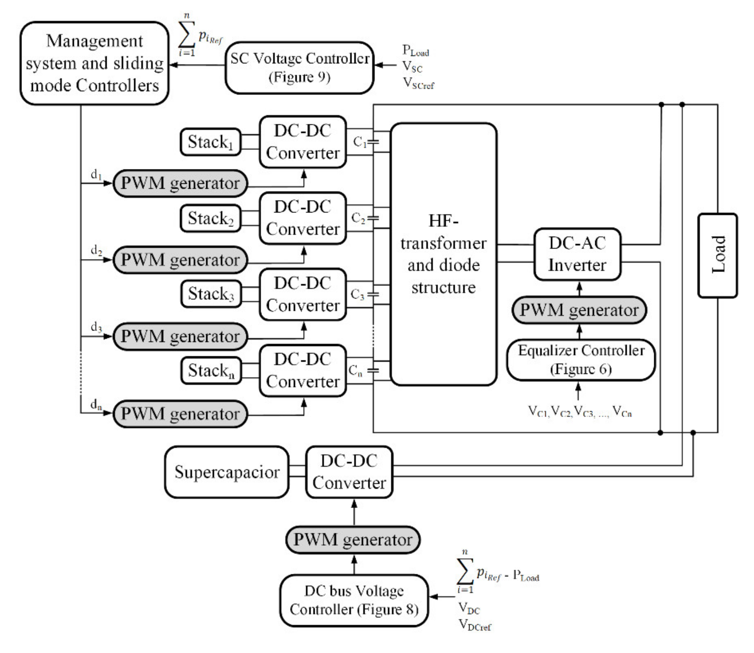
2. Proposed System Configuration

The proposed power electronic architecture used to realize the fuel cell management system is shown in Figure 3. As seen in this figure, the N fuel cell stacks are used and connected to the DC link through the DC–DC boost converters. Inspired by the cascade topology, the output capacitors of the boost converters are connected in series. These boost converters allow the separate management of those stacks. To ensure the controllability of different boost converters, an equalizer architecture based on the multi-winding transformer is used in this paper. Indeed, the input of the H-bridge inverter is connected to the DC-link where a capacitor CH is used to stabilize the voltage. The H-bridge inverter converts this DC voltage to an AC voltage at the input of the HF transformer. The diode structure at the output of the HF transformer allows the transmission of energy from AC secondary windings to the lower voltage capacitors. The equalizer architecture was deeply investigated and verified by experimental results in [31] without hybridization. To regulate the DC bus voltage, the SC with the conventional bidirectional boost converter is used. In order to realize the whole system, each part is modeled separately.

2.1. Model of the Equalizer

As shown in Figure 3 H-bridge inverter is connected to the primary side of a High Frequency (HF) transformer. To stabilize the input voltage of the H-bridge inverter, a capacitor (CH) is used. A special diode structure is used on the secondary side of the transformer. This topology allows the energy to be transferred from the DC-link to the lower voltage capacitors.
The following assumptions are considered for the purpose of simplicity:
(1)
Turn ratio for all secondary windings are the same and equal to m = N 2 k   N 1 and k is the coupling coefficient.
(2)
The coupling coefficient between the primary and secondary windings are identical and equal to k.
(3)
The coupling coefficient between the secondary windings is unitary.
(4)
The DC bus voltage is controlled to a reference constant value.
(5)
The switches are considered as the ideal devices. The diode voltage drops are taken into account but their dynamical resistance is assumed zero.
The theoretical waveforms of the proposed equalizer in steady-state are shown in Figure 4a. when C1 (and C2) are the lower voltage capacitors between odd and even-numbered capacitors respectively. As seen in this figure, based on the proposed switching commands for the H-bridge inverter, a symmetrical square waveform (Vin) is imposed on the primary side of the HF transformer with a variable duty cycle (d). Therefore, the odd\even numbered diodes can be naturally turned on during the positive\negative part of this square wave because of the diode structure and the polarity of secondary windings. The diode corresponding to the lower voltage capacitor between odd\even numbered diodes is automatically turned on during the positive\negative part of the input voltage of the HF transformer. Due to the same polarity of the secondary windings, a voltage equal to the lower voltage between the odd\even numbered capacitor voltages is induced to all windings when an odd\even numbered diode starts to conduct. Therefore, other odd\even numbered diodes are negatively biased during the conduction of one diode.
Theoretical waveforms of the proposed equalizer are shown in Figure 4a when the first capacitor has the lowest voltage and in Figure 4b when the first and second capacitors have the lower voltage between odd\even numbered capacitors and other capacitors have the same voltage. As seen in those figures, the transformer current waveform can be symmetrical or not. To be more general, the second case is presented as the operation modes as follows:
(1)
Mode 1 [t0–t1: Figure 5a]: Based on the switching command of the H-bridge inverter, a positive voltage is imposed on the primary side of the transformer. Regarding the assumption that the first capacitor has the lower voltage between the odd-numbered capacitor, the first diode is turned on and the derivative equation of the system is as follows:
L m d i m d t = V C 1 + V d m L f d i f d t = V i n V C 1 + V d m r f i f C 1 d V C 1 d t = i f i m V C 1 + V d m r m m i l o a d + P 1 V C 1 C j d V C j d t = P j V C j i l o a d j = 2 , 3 , 4
where Lm and Lf are, respectively, the magnetic and leakage inductances, rm and rf are the magnetic and leakage resistances, im is the magnetizing current, if is the leakage current, Vd is the diode drop voltage, Vin is the input voltage at the primary side of the transformer, Vcj is the voltage of Cj, Pj is the injected power by the boost converter corresponding to the jth fuel cell, and iload is the load current.
(2)
Mode 2 [t1–t2: Figure 5b]: The input voltage of the HF transformer is equal to zero in this mode. D1 can continue to conduct during the interval of [t1,tf] and, as a result, the derivative equations of the system are as follows:
L m d i m d t = V C 1 + V d m L f d i f d t = V C 1 + V d m r f i f C 1 d V C 1 d t = i f i m V C 1 + V d m r m m i l o a d + P 1 V C 1 C j d V C j d t = P j V C j i l o a d j = 2 , 3 , 4
The switching frequency of the H-bridge inverter is low enough that the diode can be turned off before the end of this mode. As a result, the derivative equations of the system during the interval of [tf,t2] are as following when the diode is off:
L m d i m d t = r m i f i m L f d i f d t = r f i f r m i f i m C j d V C j d t = P j V C j i l o a d j = 1 , 2 , 3 , 4
(3)
Mode 3 [t2–t3: Figure 5c]: A negative voltage is imposed on the primary side of the HF transformer in this mode. As a result, the second diode corresponding to the lower voltage capacitor among even-numbered capacitors starts to conduct. The derivative equations of the system are as follows:
L m d i m d t = V C 2 + V d m L f d i f d t = V i n + V C 2 + V d m r f i f C 2 d V C 2 d t = i f i m + V C 2 + V d m r m m i l o a d + P 2 V C 2 C j d V C j d t = P j V C j i l o a d j = 1 , 3 , 4
It can be noted that this mod does not exist for Figure 4a.
(4)
Mode 4 [t3–t4: Figure 5d]: This mode is similar to mode 2 but due to negative voltage imposed on the primary side of the HF transformer, the even-numbered diodes can be turned on. Since the second capacitor is assumed to be the lower voltage capacitor between the even-numbered capacitors, the second diode begins to conduct the current. The derivative equation of the system before the diode stops to conduct is as following during the interval of [t3,tfe]:
L m d i m d t = V C 2 + V d m L f d i f d t = V C 2 + V d m r f i f C 2 d V C 2 d t = i f i m + V C 2 + V d m r m m i l o a d + P 2 V C 2 C j d V C j d t = P j V C j i l o a d j = 1 , 3 , 4
Over the interval of [tfe,t4] the derivative equations of the system are changed as (4) when the diode D2 is off in this mode. Moreover, this mod does not take place for Figure 4a.
Based on these modes, the power can be transferred from the series connection of capacitors to the lower voltage capacitors. Further information and details about this equalizer can be found in [31].

2.2. Improved Control Method for the Equalizer

As seen in Figure 6, the maximum voltage among the output capacitors connected to the boost converters of different stacks is compared with the lowest voltage and this difference is multiplied by the proportional gain to obtain the duty cycle. Compared to [31], this controller is also able to decrease the maximum voltage on each output capacitor and can consequently reduce the stress on the capacitors and semiconductor devices. A low-pass filter is used in this controller to optimize the dynamical behavior of the equalizer. Due to the possibility of a large external perturbation during the transient states, this controller can impose a high value of duty cycle that leads to conduct a high value of current in semiconductors. Using a dynamic saturation can cope with this issue. To model such a control system, the derivative equation of the filter is used as follows:
d y d t = ω f V C max V C min y
where y is the output of the filter, ω f is the cut-off frequency of the filter, V C min and V C max are the minimum and maximum voltages among the capacitor voltages, respectively. The difference between the maximum and the minimum voltages is used as the input of the filter. As a result, the duty cycle of the H-bridge inverter is calculated as follows:
d = K p y
In this paper, a protection circuit is also proposed to dynamically control the maximum value of the duty cycle and indirectly control the maximum value of the current. As seen in Figure 6, this protection is implemented by considering the derivative equation of leakage inductance of the transformer. Based on Figure 4, the leakage current of the transformer can be positively\negatively reached to its maximum during the positive\negative part of the input voltage of the transformer. The time interval of [t0,t1] or [t2,t3] is equal to dT/2 where T is 1/F and F is the switching frequency. Therefore, the maximum duty cycle can be deduced from the model as following regardless of the losses:
L f I m a x d T / 2 = Δ V

2.3. Average Model

Considering the supplied power by the first stack is lower than the others, the first capacitor voltage has the lowest voltage. The other stacks inject the nominal power and as a result, the output capacitors of their boost converters have the same voltage. A dynamical average model can be considered for this system by calculating the transmitted power through the transformer. To calculate this power, the diode current equation can be used. Based on the approach in [31], an equation for the transmitting power through the transformer can be obtained as follows:
P e 1 = d V C 1 8 F 2 m 2 ( d F m V d c B 1 L f d F B 1 L m 16 F 3 L m m r m V d c 2 L f B 1 r m 4 F L f L m + 4 F L C r m d r f r m   + d 2 F r f m r m V d c + 2 L f B 1 L f 4 F L f L m 4 F L C r m + d r f r m d 4 F L C + 2 d r f   A 1 4 L f L m B 1 4 F L f L m 4 F L C r m + d r f r m 2 )
This power is received by the first capacitor. A similar equation can be obtained for the transferred power to one of the even-numbered capacitors. Considering the second capacitor as a lower voltage capacitor among the even-numbered capacitors, the transferred power can be calculated as follows:
P e 2 = d V C 2 8 F 2 m 2 ( d F m V d c B 2 L f d F B 2 L m 16 F 3 L m m r m V d c 2 L f B 2 r m 4 F L f L m + 4 F L C r m d r f r m   + d 2 F r f m r m V d c + 2 L f B 2 L f 4 F L f L m 4 F L C r m + d r f r m d 4 F L C + 2 d r f   A 2 4 L f L m 4 F L f L m 4 F L C r m + d r f r m 2 B 2 )
This power is received by the second capacitor. It can be noted that this power is negligible in the case of Figure 4a.
To obtain a dynamical average model, the power that is consumed by the equalizer is also required. To calculate this power, the losses inside the system should be added to P e 1 + P e 2 . The injected power to the equalizer can be calculated as follows:
P i n = P e 1 + P e 2 + V ¯ p 1 2 + V ¯ p 2 2 r m + r f I ¯ f 1 2 + I ¯ f 2 2
where I ¯ f 1 is the RMS value of the leakage current of the transformer due to the transmitting energy to the first capacitor, and V ¯ p 1 is the RMS voltage on the primary side of the transformer due to the transmitting energy to the first capacitor that is the RMS value of V d + V C 1 m over the interval of tf-t0 in the switching period as follows:
I ¯ f 1 2 = 1 T t 0 t f i f t 2 d t = 1 T t 0 t 1 i f t 2 d t + t 1 t f i f t 2 d t V ¯ p 1 2 = 1 T t 0 t f V d + V C 1 m 2 d t = t f t 0 T V d + V C 1 m 2
where I ¯ f 2 and V ¯ p 2 are the RMS values of the leakage current of the transformer and the RMS voltage on the primary side of the transformer due to the transmitting energy to the second capacitor that can be calculated in a similar way in the interval of [t2,tfe]. It can be noted that this current is negligible in the case of Figure 4a. The load current that is seen by the series connection of the capacitors can be calculated regarding the injecting power to the equalizer as follows:
i c h = i l o a d + P i n V d c i a
where iload is the load current, and ia is the current that is injected by the SC.
Calculating the received power by the capacitors, a dynamical average model based on the derivative equations of the system can be obtained as follows:
C 1 d V C 1 d t = P 1 + P e 1 V C 1 i c h C 2 d V C 2 d t = P 2 + P e 2 V C 2 i c h C j d V C j d t = P j V C j i c h     j 3 , 4 , , n
To control the power delivered by each stack, the sliding mode controller is used. This control is explained in the following section. The parameter of this controller is chosen in such a way that this controller is only as fast as required. Therefore, the reference power is always followed by this controller.

3. Hybridization

The diagram of the overall control structure is shown in Figure 7. As seen in this figure, each part of the system is controlled by its own controller. In this section, the method of regulating the DC-link and the SC voltages will be detailed. This method is based on an energy regulator (extern loop) and an indirect sliding mode control. This simple method can ensure that the dynamic performances are independent of the operating points.

3.1. DC Bus Voltage Controller

To regulate the DC bus voltage, an SC is connected to the DC bus by a bidirectional boost converter. The state-space model of the super-capacitor with a boost converter is as follows:
L S C d i S C d t = v s c 1 d S C V d c r S C i S C C S C d v S C d t = i S C
where Lsc is the inductance connected to the boost converter of the SC and rsc is its resistance, vsc is the SC voltage, and isc is its current. Therefore, the injected current to the DC bus by the SC can be calculated as follows:
i a = 1 d S C i S C
To control the DC bus voltage, a controller based on the flatness theory is used in this paper. This controller is deeply studied in [51,52]. The stored energy in the DC link is used as the output variable of this controller. This energy can be calculated as follows:
y d c = 1 2 C e q V d c 2
where Ceq is the equivalent capacitor of series-connected capacitors. The derivation of this energy is as follows:
y ˙ d c = j = 1 n P j + P a P l o a d
where Pa is the power injected to DC bus by the SC. Hence:
P a = y ˙ d c + P l o a d j = 1 n P j
Considering the losses of the boost converter in the resistance of its inductance, this power can be calculated as follows:
P a = P S C r S C P S C v s c 2 L S C P S C v s c d S C P S C v s c d t
where Psc is the injected power by the SC. As seen in Figure 8, this control is realized by two loops. The inner loop is the power loop and the energy loop is an outer loop. Based on the energy stored in the DC bus, the energy loop can control the voltage of the DC bus. Assuming that the outer loop (energy loop) is slower enough than the inner loop (power loop), the variation of the magnetic energy can be neglected. Furthermore, the injected power by SC can be rewritten as follows:
P S C = 2 P m a x 1 1 P a P m a x
where Pmax is as follows:
P m a x = v S C 2 4 r S C
Using (19)–(23), the power that must be injected by the SC to regulate the DC link voltage is obtained. This control can operate when the inner loop, which controls the power of SC, is fast enough. To ensure that the electrostatic energy follows its reference, a control method based on the second-order system is used as follows [53]:
y ˙ d c r e f y ˙ d c + K 1 y d c r e f y d c + K 2 y d c r e f y d c = 0
where K1 and K2 are the controlling parameters with K 1 = 2 ζ ω n , and K 2 = ω n 2 (where ω n is the desired cutoff radian frequency of the voltage control loop [53]). y ˙ d c is obtained from (24). (20) and (24) allow the SC power reference to be obtained. The inner loop goal is to control the power delivered by the SC to track its reference.
Assuming that the dynamic of the SC voltage variations is slow in comparison to the DC bus voltage variations, the SC voltage can be considered as a constant value for the design of the DC bus control. As a result, the reference current of the SC can be obtained by dividing its reference power to its voltage. The sliding mode control method is used in this study to control the current.
A sliding surface is defined as follows [54]:
s = i S C i S C r e f + k i i S C i S C r e f
To ensure the zero steady-state error, an integral term is used in this sliding surface [54]. The associated reaching condition is defined as follows:
s ˙ x = λ s x
where λ is a positive constant that determines the speed of attraction to the sliding surface. Using this approach, two poles of the system are λ and k i and independent of the operating point. By differentiating (25) and using (26), the following equation is obtained:
d i S C d t + k i i S C i S C r e f = λ s x
Using this equation and (16), the equivalent duty cycle of the SC converter can be calculated as follows:
d S C = L S C V d c V d c v s c + r S C i S C L S C k i i S C i S C r e f λ i S C i S C r e f + k i i S C i S C r e f

3.2. SC Voltage Controller

A similar approach is used to control the voltage of SC. The stored energy in SC is used to controls its voltage. This energy can be calculated as follows:
y S C = 1 2 C S C v s c 2
where CSC is the capacitance of the SC. Considering that the dynamic of the DC bus voltage loop is widely greater than the dynamic of the SC voltage, the derivation of this energy is as follows:
y ˙ S C = P S C j = 1 n P j P l o a d
where y ˙ S C is the power of the SC (PSC) that should be transferred to the SC (negative) or injected by it (positive). The total power of stacks that must be injected in steady-state can be obtained by this equation. A simple proportional gain controller is used to ensure that stored energy in the SC follows its reference:
y ˙ S C r e f y ˙ s c + K sc y S C r e f y S C = 0
The proportional gain KSC, which represents the cutoff radian frequency of the SC voltage loop, should respect the low dynamic assumption of the SC voltage. Based on (30), the total power that should be injected by the stacks can be calculated. As seen in Figure 9, a rate limiter is used to respect the dynamical constraint imposed by the fuel cell auxiliaries. Vi and ii are the voltage and current of the ith stack. di is the duty cycle of the boost converter connected to the ith stack.

4. Simulation and Experimental Results

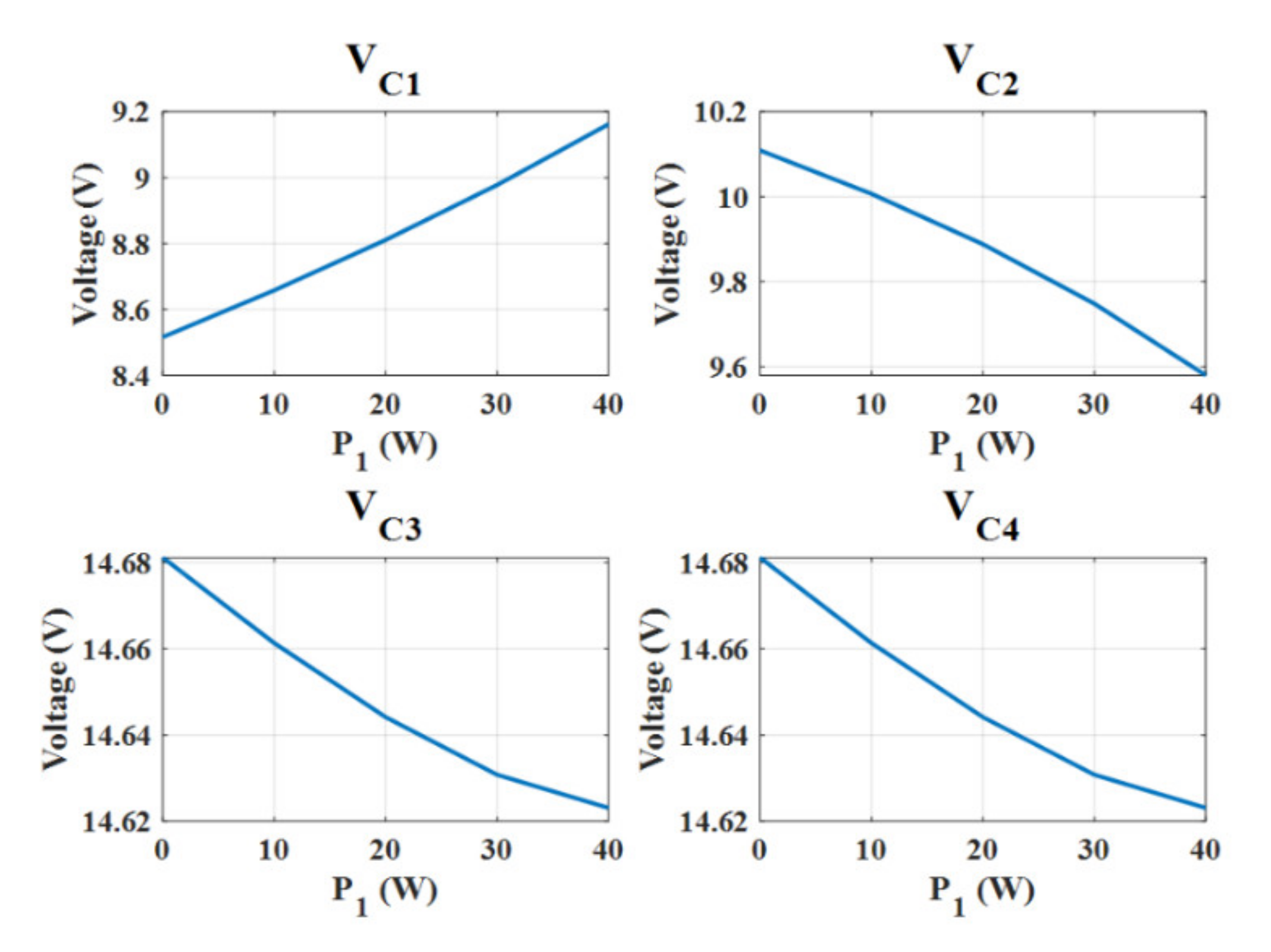
4.1. Simulation Results

To evaluate the behavior of the dynamical average model, two simulations are performed when four stacks are connected to four boost converters. The injected power by the first stack is changed from 63 to 100 W at 0.05 s while the first simulation. The injected power of the other stacks is fixed to nominal power (126 W) during this simulation.
The parameters used to obtain simulation results are shown in Table 1. To study the dynamical behavior of the average model, the state-space model of the system based on (1)–(5) is also simulated with the same parameters. The results of the first simulation are shown in Figure 10. As seen in these figures, the average model results are consistent with the results of the state space model. The voltage change of the output capacitor of the boost converters connected to the different stacks is shown in Figure 10. The difference between the two models is due to the linearizing method which was used to calculate (10). Indeed, the transformer current has an exponential form which has been approximated by the first-order polynomial based on the Taylor series. For the proposed average model, the power of the balancing system defined by (10) is a bit overestimated; consequently, the obtained voltage is a bit higher than the switching model. The voltage of the DC bus ( j V C j ) is shown in Figure 1b during this simulation. As seen in this figure, the DC voltage is regulated at the reference voltage (48 V). It is notable that the power of the fuel cell is reduced slowly and this undershoot is eliminated when the real low dynamic of the fuel cell is taken into account. Therefore, this simulation was accomplished in the worst condition.
The condition for the second simulation is similar to the first simulation except for the injected power by the second cell. This power is set to 100 W in the second simulation. The voltage changes of different capacitors are shown in Figure 11a. The DC bus voltage is shown in Figure 11b during this simulation. As seen in these figures, the average model is in agreement with the state-space model of the system.

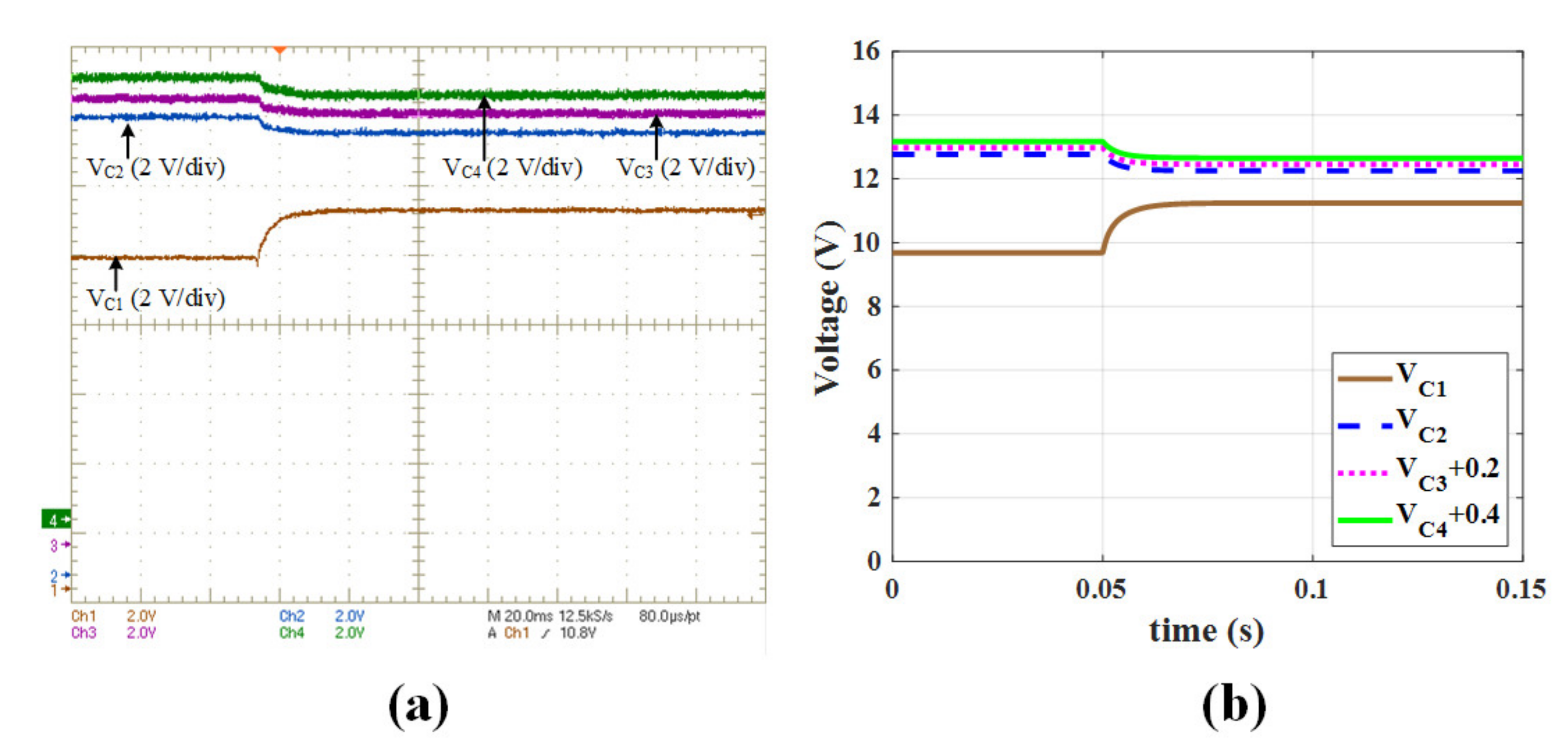
4.2. Experimental Results

To verify the validity of the proposed dynamical average model, two experiments are accomplished on a laboratory test bench as seen in Figure 12. Four different power supplies are used to emulate the four stacks of PEMFCs. dSPACE 1005 with the FPGA board is used to receive the information and send the commands. The part number of all the components is summarized in Table 2.
The same assumption of the first simulation is used to accomplish the first experiment. The experimental results of the output capacitors voltage changes are shown in Figure 13a when the first cell power is increased from 63 to 100 W. As seen in this figure, the voltage of the first capacitor is increased because of the increasing the corresponding stack injected power. The voltage of the other capacitors changed in such a way that the sum of voltage is fixed to 48 V. The average model results are also shown in Figure 13b in the same conditions for a better view. These results are verified by the experimental results. There is always an error between the simulation and experiment results in steady-state. The error between voltages of the capacitors is in a reasonable range and less than 3%. This error is caused by not considering all losses.
The second experiment is accomplished in the same conditions as the second simulation. The experimental results of the voltage changes of output capacitors are shown in Figure 14a. To provide a better view, the average model results are also shown in Figure 14b in the same conditions. As seen in this figure, the experimental results are in agreement with the simulation results. Based on the experimental and simulation results, the proposed model for the management system is valid and it can be used to study and analyze the stability of the system.

5. Stability Analysis and Energy Management

In this section, the stability of the proposed control method will be investigated. Then, the effectiveness of the proposed system in supplying the load profiles even while curing one of the stacks in two different conditions. Finally, the robustness of the proposed control method will be studied. Since the average model is valid and it can estimate the behavior of the system in closed-loop, this model can be used to analyze the stability of the system. By obtaining the eigenvalues of the Jacobian matrix of the proposed dynamical average model, the local stability around the equilibrium point can be analyzed. Furthermore, this model can be used to size the parameters of the different controllers in such a way that the stability of the system is ensured. The poles of the sliding mode controller (current controller) should be at least less than one-tenth of the switching radian frequency of the boost converters or bidirectional converter connected to the SC. The switching frequency of these converters is equal to 30 kHz. Therefore, the λ and ki of the sliding mode controller are fixed to 7500 rad/s. As mentioned before, the power loop of the DC bus voltage controller should be faster than the energy loop. As a result, the radian frequency of the energy loop should be slower than one-tenth of the current control loop. Therefore, ω n equal to 500 rad/s is used to obtain K1 and K2. The damping ratio of 0.7 is used to obtain the best behavior. The control of the SC voltage should respect the slow dynamic of the fuel cell. A rate limiter of 4 A/s limits the dynamic of current change to respect the dynamic of the fuel cell. The equalizer system controller should be faster than the DC link voltage controller to ensure the controllability of boost converters even in transient conditions. However, the cut-off frequency of the equalizer controller should be lower than one-tenth of its switching radian frequency. The switching frequency of the H-bridge inverter is equal to 40 kHz. There is a tradeoff between the dynamic of the equalizer controller and the time that the duty cycle of the H-bridge inverter is stuck in the maximum value due to the dynamic saturation. As a result, the cut-off frequency of 2π 103 rad/s is used for the equalizer controller. The dynamic variations of the SC voltage will be neglected in the stability study due to the slow dynamic of the SC voltage and the powers delivered by the fuel cells are supposed to be constant.
To evaluate the stability of the system, the power of the first cell is changed from 0 to 100 W with steps of 10 W. The other cell powers are fixed to 126 W. The other parameters that are used for this simulation is shown in Table 1. Using the proposed dynamical average model, the steady-state voltages of the boost output capacitors are shown in Figure 15. for this simulation. As seen in this figure, the voltage of the first cell is increased by increasing the injected power of the first cell. The voltage of other stacks is decreased to fix the DC bus voltage to 48 V. The eigenvalues of the closed-loop system are depicted in Figure 16. This figure shows the eigenvalues of the Jacobian matrix of the proposed dynamical average model when the stacks inject the nominal power except the first stack. As mentioned above, the injected power of the first stack is changed from zero to 100 W. These eigenvalues with negative real parts prove the stability of the system. As seen in this figure, the different groups of eigenvalues are shown in different circles with different colors and numbers. The purple circles show the eigenvalues that strongly depend on the parameters of the voltage and current controllers. The place of eigenvalues inside the purple circle numbered 1 and 2 can be changed by changing the parameters of the current sliding mode controllers. The multiple eigenvalues in the same place are shown by a circle around the multiplication sign as shown in circle number one. The place of eigenvalues inside purple circle number three and two can be changed by changing the natural radian frequency of the second-order system used to find K1 and K2 in (24). The blue circles specify the place of eigenvalues that depend on the parameters of the equalizer system controller. The place of eigenvalues inside blue circle number four can be changed by the operating point and all parameters of equalizer controller consist of the proportional gain and the cut-off frequency used for finding the duty cycle of the H-bridge inverter. The place of eigenvalues inside blue circle number five strongly depends on the operating point and the proportional gain (Kp) of the equalizer system controller.
To prove the stability of the system when two stacks are in the fault conditions, the power of the second stack is fixed to 50 W that is a little bit lower than the half of nominal power. The injected power of the first stack is increased from 0 to 40W while the injected power by the other stacks is set to 126 W. Using the proposed dynamical average model, the steady-state value of the output capacitor voltages by changing the injected power of the first stack is shown in Figure 17. As seen in this figure, the voltage of the first cell is increased by increasing the injected power of the first cell. The voltage of other stacks is decreased to fix the DC link voltage near 48 V. The eigenvalues of the closed-loop system are shown in Figure 18. This figure shows the eigenvalues of the Jacobian matrix of the proposed dynamical average model when the second stack injects 50 W and the other stacks inject the nominal power except the first stack. As mentioned above, the supplied power by the first stack is changed from zero to 50 W. These eigenvalues with negative real parts prove the stability of the system.
Regarding the stability of the system, this topology can be used to manage the cells of a stack. To evaluate the effectiveness of the proposed topology in terms of energy management and dynamic performance, three different experiments are performed. Using the test bench shown in Figure 12, these three experiments are performed in the following condition. A step of 400 W for eight seconds is applied to the baseload power in these three experiments. The four stacks are in the normal condition for the first experiment. The load power and the injected power by the first and second stack are shown in Figure 19a,b. The behavior and magnitude of the injected power by two other stacks is very close to the second stack. As seen in this figure, the injected power by the SC is increased rapidly to control the DC link voltage. The injected power by the stacks gradually increased to control the voltage of the SC. Since the load step power is very high, the injected power increased to their maximum power. The difference between the load power and injected power by the stacks is compensated by the SC. Because of the low dynamic of the fuel cells, the injected power by the stacks is gradually decreased and the SC attracts the excess amount of power injected by the stacks whereas the load power decreased to its nominal value. As seen in Figure 19a, the injected power by the SC is equal to zero in steady-state. To provide a better view during the transient conditions of the first experiment, the load power and injected power by the stacks and SC are shown in Figure 19b with the time scale of 4 s/div. The DC link and SC voltages are shown in Figure 19c during this experiment. As seen in this figure, the DC link voltage is well controlled and has a constant value of 48 V. The SC voltage is gradually decreased due to its injected power but then it increased gradually due to the increase of the injected power by the stacks and decrease of load power to its nominal value. To assess the behavior of the DC link voltage controller in transient condition, the SC injected power and the DC link and SC voltages are shown in Figure 19d with the time scale of 4 ms/div. As seen in this figure, the DC link voltage decreases due to the step of load power but the fast increase in the injected power by the SC can compensate the required load power and regulate the DC link voltage. Furthermore, the SC voltage in this figure is in agreement with the SC constant voltage assumption over the transient conditions.
In the second experiment, it is assumed that the first stack is in the drying condition whereas the other stacks are in the normal condition. To produce more water in the first stack, its current should be controlled close to its maximum in the worst condition. As seen in Figure 20a, the injected power by the first stack is controlled close to its maximum (240 W) during this experiment. A zoom is realized on the transient condition of the injected power by the SC and stacks in Figure 20b. As seen in Figure 20c, the DC link voltage is well controlled and it has a constant value of 48 V. The SC voltage is reduced due to its injected power to supply the overload. The SC voltage gradually increased and approaches to its nominal value of 24 V by increasing the injected power of stacks and decreasing the load power to its nominal value. The voltage of the output capacitors of the boost converters is shown in Figure 20d. Since the step load leads to an increase in the injected power by the stacks, the output capacitor voltages increase. The first stack injects the maximum power during this experiment. Therefore, the first capacitor voltage decreases because of the DC link voltage stabilization by the SC. The output capacitors have an identical voltage when the injected power by the stacks reach to their maximum power. The difference between the voltages at this point is originated from the losses difference in the boost converters. The injected power by the different stacks except the first stack is gradually decreased when the load power decreases to its nominal value. As a result, the difference between the first output capacitor and the other output capacitors increases. Notable that the voltage of the first stack in the drying condition is kept in an acceptable range due to the improved equalizer controller.
It is assumed that the first stack is in the flooding condition during the third experiment. The other stacks are in normal condition. In this case, the water production inside the cells of the first stack should be reduced. Therefore, the current or power injected by the first stack should be controlled close to zero in the worst condition. The equalizer ensures the controllability of the boost converters in such conditions. As seen in Figure 21a, the injected power by the first stack is controlled at zero Watt during this experiment. More details of the injected power by the SC and stacks are demonstrated in Figure 21b. Most of the overload is supplied by the SC due to the no injected power of the first stack and limits in the maximum injected power by the stacks. As a result, the SC voltage reduces more than the two previous experiments as shown in Figure 21c. The DC link voltage is also shown in this figure and it is controlled at 48 V. The voltage of the output capacitors is shown in Figure 21d during this experiment. Due to the use of the equalizer system, despite the lack of power injection by the first stack in this experiment, the first capacitor has a voltage of 10 V. This experiment confirms the function of the used equalizer system to ensure the controllability of the boost converters.
The other issue that needs to be addressed is the robustness of the control method. Robustness is the ability of the closed-loop system in being insensitive to perturbations and tolerating the component variation. To assess the robustness of the controller, the eigenvalues of the system are studied under changing some parameters of the system. If the real part of eigenvalues remains negative, it can be proved that it is a robust controller. In this system, the capacitor change can have an important effect on the stability of the system. The capacitance can be changed by aging and temperature effect. The optimum value of the capacitance is also a key factor in reducing the size of the system. In [51], a method was proposed to calculate the minimum value of the equivalent DC-link capacitance. Based on this method and assuming that the maximum permitted voltage drop in DC link is 7 V, the minimum value of each four capacitors in series connection should be 4.7 mF to tolerate a variation of the load power from −400 to 400 W.
To check the robustness of the control method, the capacitance of the first capacitor is changed from 2.35 mF to 9.4 mF. The injected power of the first cell is fixed to zero Watt and the other stacks inject the nominal power. The same parameters as Table 1 are used for the controller. The evolution of the eigenvalues of the system is depicted in Figure 22. This figure shows the eigenvalues of the Jacobian matrix of the proposed dynamical average model when the stacks inject the nominal power except the first stack. The first stack injects no power and the first capacitor value is changed as mentioned earlier. The dominant eigenvalue of the system becomes less negative by further decreasing the capacitance value from 4 mF. The place of multiple eigenvalues that are seen in this figure strongly depends on the control parameters and operating point or other parameters such as the coupling coefficient.
Another parameter that its value can have an impact on stability is the coupling coefficient between the windings of the transformer. To evaluate the impact of this parameter, the power of the first stack is fixed to zero Watt while the other stacks inject the nominal power. The coupling coefficient is changed from 0.7 to 0.97. The parameters of the controller are as same as before. The dominant eigenvalue of the system is depicted in Figure 23. This figure shows the eigenvalues of the Jacobian matrix of the proposed dynamical average model when the stacks inject the nominal power except the first stack. The first stack injects no power and the coupling coefficient value is changed as mentioned earlier.
As seen in the previous results, the real part of the eigenvalues of the system has always a negative value of less than −50. Therefore, the system is stable for a wide range of parameters change. This value depends strongly on the equalizer controller parameters.

6. Conclusions

In this paper, a power electronic system is proposed to enhance the durability of the fuel cells in multi stack architecture. Using this architecture, energy management can be performed even in the fault mode of stack and while the system is trying to cure a stack. To investigate the dynamical properties of the system and to prove its stability, a dynamical average model is proposed taking into account the order reduction induced by the presence of the HF transformer and cross-coupling effects due to the serial connection of output capacitors. The validity of the reduced model is verified through the simulation and experimental results. The stability analysis based on the proposed model proved the asymptotic stability of the system in different conditions. The robustness of this control method was also investigated based on the stability analysis by changing system parameters. The experimental results, which show the behavior of the system in different operating conditions, validated the effectiveness of the proposed topology and its associated energy management functionalities. These results also confirmed that the controllability and the DC-link voltage regulation are always ensured even during drying or flooding conditions concerning one of the stacks in which the power injected by each stack is modified to improve durability.

Author Contributions

Conceptualization, M.B. and S.P.; Data curation, M.B.; Formal analysis, M.B., S.P. and M.Z.; Funding acquisition, S.P.; Investigation, M.B. and S.P.; Methodology, M.B., S.P. and F.M.-T.; Project administration, G.M. and S.P.; Resources, S.P., and M.W.; Software, M.B.; Supervision, J.-P.M., G.M. and S.P.; Validation, M.B. and S.P.; Visualization, M.B.; Writing—original draft, M.B.; Writing—review & editing, M.B., J.-P.M., G.M. and S.P. All authors have read and agreed to the published version of the manuscript.

Funding

This research received no external funding.

Conflicts of Interest

The authors declare no conflict of interest.

References

  1. Bizon, N.; Thounthong, P. Energy efficiency and fuel economy of a fuel cell/renewable energy sources hybrid power system with the load-following control of the fueling regulators. Mathematics 2020, 8, 151. [Google Scholar] [CrossRef] [Green Version]
  2. Zandi, M.; Bahrami, M.; Eslami, S.; Gavagsaz-Ghoachani, R.; Payman, A.; Phattanasak, M.; Nahid-Mobarakeh, B.; Pierfederici, S. Evaluation and comparison of economic policies to increase distributed generation capacity in the Iranian household consumption sector using photovoltaic systems and RET Screen software. Renew. Energy 2017, 107, 215–222. [Google Scholar] [CrossRef]
  3. Bahrami, M.; Gavagsaz-Ghoachani, R.; Zandi, M.; Phattanasak, M.; Maranzanaa, G.; Nahid-Mobarakeh, B.; Pierfederici, S.; Meibody-Tabar, F. Hybrid maximum power point tracking algorithm with improved dynamic performance. Renew. Energy 2019, 130, 982–991. [Google Scholar] [CrossRef]
  4. El-fergany, A.A.; Hasanien, H.M.; Agwa, A.M. Semi-empirical PEM fuel cells model using whale optimization algorithm. Energy Convers. Manag. 2019, 201, 112197. [Google Scholar] [CrossRef]
  5. Parol, M.; Wójtowicz, T.; Księżyk, K.; Wenge, C. Optimum management of power and energy in low voltage microgrids using evolutionary algorithms and energy storage. Int. J. Electr. Power Energy Syst. 2020, 119, 105886. [Google Scholar] [CrossRef]
  6. Lan, T.; Strunz, K. Modeling of multi-physics transients in PEM fuel cells using equivalent circuits for consistent representation of electric, pneumatic, and thermal quantities. Int. J. Electr. Power Energy Syst. 2020, 119, 105803. [Google Scholar] [CrossRef]
  7. Yoshida, T.; Kojima, K. Toyota MIRAI fuel cell vehicle and progress toward a future hydrogen society. Interface Mag. 2015, 24, 45–49. [Google Scholar] [CrossRef]
  8. Matsunaga, M.; Fukushima, T.; Ojima, K. Powertrain system of Honda FCX clarity fuel cell vehicle. World Electr. Veh. J. 2009, 3, 820–829. [Google Scholar] [CrossRef] [Green Version]
  9. Wang, J. System integration, durability and reliability of fuel cells: Challenges and solutions. Appl. Energy 2017, 189, 460–479. [Google Scholar] [CrossRef]
  10. Zhang, H.; Li, X.; Liu, X.; Yan, J. Enhancing fuel cell durability for fuel cell plug-in hybrid electric vehicles through strategic power management. Appl. Energy 2019, 241, 483–490. [Google Scholar] [CrossRef]
  11. Samavatian, V.; Radan, A. A novel low-ripple interleaved buck—Boost converter with high efficiency and low oscillation for fuel-cell applications. Int. J. Electr. Power Energy Syst. 2014, 63, 446–454. [Google Scholar] [CrossRef]
  12. Maranzana, G.; Didierjean, S.; Dillet, J.; Thomas, A.; Lottin, O. Improved Fuel Cell. U.S. Patent WO/2014/060198, 24 April 2014. [Google Scholar]
  13. Wang, T.; Li, Q.; Yin, L.; Chen, W. Hydrogen consumption minimization method based on the online identification for multi-stack PEMFCs system. Int. J. Hydrog. Energy 2019, 4, 5074–5081. [Google Scholar] [CrossRef]
  14. Ozpineci, B. Optimum fuel cell utilization with multilevel DC—DC converters. In Proceedings of the 19th Annual IEEE Applied Power Electronics Conference and Exposition, Anaheim, CA, USA, 22–26 February 2004. [Google Scholar]
  15. Ozpineci, B.; Case, A.A. Multiple input converters for fuel cells. In Proceedings of the Conference Record of the 2004 IEEE Industry Applications Conference, Seattle, WA, USA, 3–7 October 2004. [Google Scholar]
  16. Lopes, C.; Kelouwani, S.; Boulon, L.; Agbossou, K.; Marx, N.; Ettihir, K. Neural network modeling strategy applied to a multi-stack PEM fuel cell system. In Proceedings of the 2016 IEEE Transportation Electrification Conference and Expo (ITEC), Dearborn, MI, USA, 27–29 June 2016; pp. 1–7. [Google Scholar]
  17. Ramadan, H.S.; de Bortoli, Q.; Becherif, M.; Claude, F. Multi-stack fuel cell efficiency enhancement based on thermal management. IET Electr. Syst. Transp. 2016, 7, 65–73. [Google Scholar]
  18. Marx, N.; Cardenas, D.C.T.; Boulon, L.; Gustin, F.; Hissel, D. Degraded mode operation of multi-stack fuel cell systems. IET Electr. Syst. Transp. 2016, 6, 3–11. [Google Scholar] [CrossRef]
  19. Cardenas, D.C.T.; Hissel, D.; Marx, N.; Boulon, L.; Gustin, F. Degraded mode operation of multi-stack fuel cell systems. In Proceedings of the 2014 IEEE Vehicle Power and Propulsion Conference (VPPC), Coimbra, Portugal, 27–30 October 2014. [Google Scholar]
  20. Garcia, J.E.; Herrera, D.F.; Boulon, L.; Sicard, P.; Hernandez, A. Power sharing for efficiency optimisation into a multi fuel cell system. In Proceedings of the 2014 IEEE 23rd International Symposium on Industrial Electronics (ISIE), Istanbul, Turkey, 1–4 June 2014; pp. 218–223. [Google Scholar]
  21. Candusso, D.; De Bernardinis, A.; Peera, M.-C.; Harel, F.; Francois, X.; Hissel, D.; Coquery, G.; Kauffmann, J.-M. Fuel cell operation under degraded working modes and study of diode by-pass circuit dedicated to multi-stack association. Energy Convers. Manag. 2008, 49, 880–895. [Google Scholar] [CrossRef]
  22. Lape, N.; Dudfield, C.; Orsillo, A. Environmentally friendly power sources for aerospace applications. J. Power Sources 2008, 181, 353–362. [Google Scholar]
  23. Miller, A.R.; Hess, K.S.; Barnes, D.L.; Erickson, T.L. System design of a large fuel cell hybrid locomotive. J. Power Sources 2007, 173, 935–942. [Google Scholar] [CrossRef]
  24. Von Helmolt, R.; Eberle, U. Fuel cell vehicles: Status 2007. J. Power Sources 2007, 165, 833–843. [Google Scholar] [CrossRef]
  25. Hamad, K.B.; Taha, M.H.; Almaktoof, A.; Kahn, M.T.E. Modelling and analysis of a grid-connected megawatt fuel cell stack. In Proceedings of the 2019 International Conference on the Domestic Use of Energy (DUE), Wellington, South Africa, 25–27 March 2019; pp. 147–155. [Google Scholar]
  26. Cardozo, J.; Marx, N.; Hissel, D. Comparison of multi-stack fuel cell system architectures for residential power generation applications including electrical vehicle charging. In Proceedings of the IEEE Vehicle Power and Propulsion Conference (VPPC), Montreal, QC, Canada, 19–22 October 2015; pp. 2–7. [Google Scholar]
  27. Wang, C.; Nehrir, M.H.; Gao, H. Control of PEM fuel cell distributed generation systems. IEEE Trans. Energy Convers. 2006, 21, 586–595. [Google Scholar] [CrossRef]
  28. Marx, N.; Boulon, L.; Gustin, F.; Hissel, D.; Agbossou, K. A review of multi-stack and modular fuel cell systems: Interests, application areas and on-going research activities. Int. J. Hydrogen Energy 2014, 39, 12101–12111. [Google Scholar] [CrossRef]
  29. Arunkumari, T.; Indragandhi, V. An overview of high voltage conversion ratio DC-DC converter configurations used in DC micro-grid architectures. Renew. Sustain. Energy Rev. 2017, 77, 670–687. [Google Scholar] [CrossRef]
  30. Wu, Q.; Member, S.; Wang, Q.; Xu, J. A high efficiency step-up current-fed push-pull quasi-resonant converter with fewer components for fuel cell application. IEEE Trans. Ind. Electron. 2016, 64, 6639–6648. [Google Scholar] [CrossRef]
  31. Bahrami, M.; Martin, J.; Maranzana, G.; Pierfederici, S.; Weber, M.; Meibody-Tabar, F.; Zandi, M. Design and modeling of an equalizer for fuel cell energy management systems. IEEE Trans. Power Electron. 2019, 24, 10925–10935. [Google Scholar] [CrossRef]
  32. Chen, Y.; Liu, X.; Cui, Y.; Zou, J.; Yang, S. A multi winding transformer cell-to-cell active equalization method for lithium-ion batteries with reduced number of driving circuits. IEEE Trans. Power Electron. 2016, 31, 4916–4929. [Google Scholar] [CrossRef]
  33. Sulaiman, N.; Hannan, M.A.; Mohamed, A.; Ker, P.J.; Majlan, E.H.; Wan Daud, W.R. Optimization of energy management system for fuel-cell hybrid electric vehicles: Issues and recommendations. Appl. Energy 2018, 228, 2061–2079. [Google Scholar] [CrossRef]
  34. Lü, X.; Wu, Y.; Lian, J.; Zhang, Y.; Chen, C.; Wang, P.; Meng, L. Energy management of hybrid electric vehicles: A review of energy optimization of fuel cell hybrid power system based on genetic algorithm. Energy Convers. Manag. 2020, 205, 112474. [Google Scholar] [CrossRef]
  35. Marzougui, H.; Kadri, A.; Martin, J.; Amari, M.; Pierfederici, S. Implementation of energy management strategy of hybrid power source for electrical vehicle. Energy Convers. Manag. 2019, 195, 830–843. [Google Scholar] [CrossRef]
  36. Lü, X.; Qu, Y.; Wang, Y.; Qin, C.; Liu, G. A comprehensive review on hybrid power system for PEMFC-HEV: Issues and strategies. Energy Convers. Manag. 2018, 171, 1273–1291. [Google Scholar] [CrossRef]
  37. Marx, N.; Hissel, D.; Gustin, F.; Boulon, L.; Agbossou, K. On the sizing and energy management of an hybrid multistack fuel cell e battery system for automotive applications. Int. J. Hydrog. Energy 2016, 42, 1518–1526. [Google Scholar] [CrossRef]
  38. Lü, X.; Wang, P.; Meng, L.; Chen, C. Energy optimization of logistics transport vehicle driven by fuel cell hybrid power system. Energy Convers. Manag. 2019, 199, 111887. [Google Scholar] [CrossRef]
  39. Zhan, Y.; Wang, H.; Zhu, J. Modelling and control of hybrid UPS system with backup PEM fuel cell/battery. Int. J. Electr. Power Energy Syst. 2012, 43, 1322–1331. [Google Scholar] [CrossRef]
  40. Li, T.; Liu, H.; Ding, D. Predictive energy management of fuel cell supercapacitor hybrid construction equipment. Energy 2018, 149, 718–729. [Google Scholar] [CrossRef]
  41. Bizon, N.; Lopez-Guede, J.M.; Kurt, E.; Thounthong, P.; Gheorghita, A.; Mihai, L.; Iana, G. Hydrogen economy of the fuel cell hybrid power system optimized by air flow control to mitigate the effect of the uncertainty about available renewable power and load dynamics. Energy Convers. Manag. 2019, 179, 152–165. [Google Scholar] [CrossRef]
  42. Bizon, N.; Cristian, I. Hydrogen saving through optimized control of both fueling flows of the fuel cell hybrid power System under a variable load demand and an unknown renewable power profile. Energy Convers. Manag. 2019, 184, 1–14. [Google Scholar] [CrossRef]
  43. Phattanasak, M.; Martin, J.; Pierfederici, S.; Davat, B. Predicting the onset of bifurcation and stability study of a hybrid current controller for a boost converter. Math. Comput. Simul. 2013, 91, 262–273. [Google Scholar]
  44. Gavagsaz-ghoachani, R.; Phattanasak, M.; Zandi, M.; Martin, J.; Pierfederici, S.; Nahid-mobarakeh, B.; Davat, B. Estimation of the bifurcation point of a modulated-hysteresis current-controlled DC—DC boost converter: Stability analysis and experimental verification. IET Power Electron. 2015, 8, 2195–2203. [Google Scholar] [CrossRef]
  45. Saublet, L.; Gavagsaz-Ghoachani, R.; Martin, J.; Nahid-mobarakeh, B.; Member, S.; Pierfederici, S. Bifurcation analysis and stabilization of DC power systems for electrified transportation systems. IEEE Trans. Transp. Electrif. 2016, 2, 86–95. [Google Scholar] [CrossRef]
  46. Mira, M.C.; Zhang, Z.; Knott, A.; Andersen, M.A. Analysis, design, modeling, and control of an Interleaved-boost full-bridge three-port converter for hybrid renewable energy systems publication date: Analysis, design, modelling and control of an interleaved-boost full-bridge three-port converter f. IEEE Trans. Power Electron. 2017, 32, 1138–1155. [Google Scholar] [CrossRef] [Green Version]
  47. Wang, L.; Member, S.; Vo, Q.; Prokhorov, A. V Dynamic stability analysis of a hybrid wave and photovoltaic power generation system integrated into a distribution power grid. IEEE Trans. Sustain. Energy 2017, 8, 404–413. [Google Scholar] [CrossRef]
  48. Yuhimenko, V.; Member, S.; Geula, G.; Member, S.; Agranovich, G.; Averbukh, M.; Kuperman, A.; Member, S. Average modeling and performance analysis of voltage sensorless active supercapacitor balancer with peak current protection. IEEE Trans. Power Electron. 2017, 32, 1570–1578. [Google Scholar] [CrossRef]
  49. Qin, H.; Kimball, J.W. Generalized average modeling of dual active. IEEE Trans. Power Electron. 2012, 27, 2078–2084. [Google Scholar] [CrossRef]
  50. Renaudineau, H.; Martin, J.; Nahid-Mobarakeh, B.; Member, S.; Pierfederici, S. DC—DC converters dynamic modeling with state observer-based parameter estimation. IEEE Trans. Power Electron. 2015, 30, 3356–3363. [Google Scholar] [CrossRef] [Green Version]
  51. Payman, A.; Pierfederici, S.; Meibody-Tabar, F.; Davat, B. An adapted control strategy to minimize DC—Bus capacitors of a parallel fuel cell/ultracapacitor hybrid system. IEEE Trans. Power Electron. 2011, 26, 3843–3852. [Google Scholar] [CrossRef]
  52. Payman, A.; Pierfederici, S.; Meibody-Tabar, F. Energy control of supercapacitor/fuel cell hybrid power source. Energy Convers. Manag. 2008, 49, 1637–1644. [Google Scholar] [CrossRef]
  53. Thounthong, P.; Pierfederici, S.; Davat, B. Analysis of differential flatness-based control for a fuel cell hybrid power source. IEEE Trans. Energy Convers. 2010, 25, 909–920. [Google Scholar] [CrossRef] [Green Version]
  54. Tabart, Q.; Vechiu, I.; Etxeberria, A.; Bacha, S. Hybrid energy storage system microgrids integration for power quality improvement using four leg three level NPC inverter and second order sliding mode control. IEEE Trans. Ind. Electron. 2018, 65, 424–435. [Google Scholar] [CrossRef]
Figure 1. Multi stack topologies: (a) Series; (b) Parallel; (c) Cascade; (d) Series-parallel.
Mathematics 08 00739 g001
Figure 2. Cascade topology with different injected powers by stacks.
Mathematics 08 00739 g002
Figure 3. Proposed power electronic architecture to realize fuel cell management system.
Mathematics 08 00739 g003
Figure 4. Theoretical waveforms in the steady-state of the proposed equalizer whereas: (a) Vc1 is the lowest voltage between all capacitors; (b) Vc1\Vc2 is the lowest voltage between the odd\even numbered capacitors.
Mathematics 08 00739 g004
Figure 5. Different operation modes of the proposed equalizer. (a) Mode 1: t0 < t < t1. (b) Mode 2: t1 < t < t2. (c) Mode 3: t2 < t < t3. (d) Mode 4: t3 < t < t4.
Mathematics 08 00739 g005
Figure 6. Schematic diagram of the control method used to determine the duty cycle (d) of the H-bridge inverter.
Mathematics 08 00739 g006
Figure 7. Diagram of the overall control structure.
Mathematics 08 00739 g007
Figure 8. Schematic diagram of the voltage controller.
Mathematics 08 00739 g008
Figure 9. Schematic diagram of the SC voltage controller.
Mathematics 08 00739 g009
Figure 10. Simulation results in closed-loop when P1 is increased from 63 to 100 W and the other stacks inject the nominal power: (a) Voltage changes of the boost converters output capacitors connected to the stacks; (b) DC bus voltage.
Mathematics 08 00739 g010
Figure 11. Simulation results in closed-loop when P1 is changed from 63 to 100 W, P2 is set to 100 W, and the other stacks inject the nominal power: (a) Voltage changes of the boost converters output capacitors connected to the stacks; (b) DC bus voltage.
Mathematics 08 00739 g011
Figure 12. Test bench of the proposed system.
Mathematics 08 00739 g012
Figure 13. Voltage changes of the boost converters output capacitors connected to the stacks in closed-loop when P1 is increased from 63 to 100 W, and P2 is set to the nominal power: (a) Experimental results; (b) Simulation results of the average model.
Mathematics 08 00739 g013
Figure 14. Voltage changes of the boost converters output capacitors in closed-loop when P1 is changed from 63 to 100 W, and P2 is set to 100 W: (a) Experimental results; (b) Simulation results of the average model.
Mathematics 08 00739 g014
Figure 15. Voltage changes of the boost converters’ output capacitor connected to fuel cell stacks in closed-loop by changing the injected power of the first stack while the other stacks inject the nominal power of 126 W.
Mathematics 08 00739 g015
Figure 16. Eigenvalues of the closed-loop system by changing the injected power of the first stack while the other stacks inject the nominal power of 126 W.
Mathematics 08 00739 g016
Figure 17. Voltage changes of the boost converters’ output capacitor connected to fuel cell stacks in closed-loop by changing the injected power of the first stack while the second stack injects 50 W and the other stacks inject the nominal power of 126 W.
Mathematics 08 00739 g017
Figure 18. Dominant eigenvalues of the closed-loop system by changing the injected power of the first stack while the second stack injects 50 W and the other stacks inject the nominal power of 126 W.
Mathematics 08 00739 g018
Figure 19. Experimental result of the energy management system when the stacks are in the normal condition and an overload occurs: (a) Injected power and load power variations; (b) Zoom on powers; (c) DC link and SC voltage changes; (d) zoom on the part c.
Mathematics 08 00739 g019
Figure 20. Experimental result of the energy management system when the stacks are in the normal condition except the first stack (drying condition) and an overload occurs: (a) Injected power and load power variations; (b) Zoom on the power; (c) DC link and SC voltage changes; (d) Output capacitor voltage changes.
Mathematics 08 00739 g020
Figure 21. Experimental result of the energy management system when the stacks are in the normal condition except the first stack (flooding condition) and an overload occurs: (a) Injected power and load power variations; (b) Zoom on the powers; (c) DC link and SC voltage changes; (d) Output capacitor voltage changes.
Mathematics 08 00739 g021
Figure 22. Dominant eigenvalues of the closed-loop system by changing the capacitance value of the first capacitor when the power of the first stack is equal to zero W and the other stacks inject the nominal power of 126 W.
Mathematics 08 00739 g022
Figure 23. Dominant eigenvalues of the closed-loop system by changing the coupling coefficient when the power of the first stack is equal to zero W and the other stacks inject the nominal power of 126 W.
Mathematics 08 00739 g023
Table 1. Parameters of the proposed equalizer.
SymbolUnitValueDescription
C μ F 4700Electrochemical
ALnH/turns212,500Planar transformer core
N1turns1Primary winding turns
N2turns4Secondary winding turns
k-0.98Coupling coefficient
FkHz40Switching frequency of the H-bridge
VbatV48Nominal voltage of the battery
VCV12Nominal output voltages of boosts
VdV0Drop voltage of diodes
PFCW126Nominal injected power of different stacks
η -1Efficiency of the equalizer system
ω f Rad/s 2 π 10 3 Cut-off radian frequency of the filter
Kp-0.1Proportional gain of the controller
λ Rad/s7500
kiRad/s7500
FskHz29Switching frequency of the boost converters
KSC-0.08
Table 2. Parameters of the used devices in the test bench.
UnitValue
FCPower supplyTDK GENH 750 W
Boost converterInductance(1 mH)
SwitchesIGBT
CapacitorElectrochemical (4700 μ F )
EqualizerDiodesDSS2x121-0045B
Magnetic coreB66295G Material N87
H-bridge switchesSiCMOSFET CCS050M12CM2
Capacitorfilm (220 μ F )

