1. Introduction
Nowadays, fossil fuels are the primary source of energy worldwide, but the extensive use of this natural resource has caused an increase in the average temperature of the earth. Environmental organizations have the aim of gradually decoupling the use of fossil fuels from 70% to 20% in 2050 [
1]. Advances in the technology directed on the energy production area, environmental sustainability, and the appearance of small generation systems have opened new opportunities to research in Distributed Energy Resources (DERs). The DERs have raised an alternative solution to efficiently face the actual energy demand, centered on the reliability and energy quality [
2]. Many consumers, such as buildings, factories, and residential neighborhoods, are planning to place a Microgrid (MG) considering the cost reductions in the technology associated with the DERs and storage systems, contributing simultaneously to reach a better energy quality [
3]. MG is defined as an interconnected load group and DERs with boundaries clearly defined that act as a controllable entity concerning the grid [
4]. MG is composed of essential components as the loads, DERs, Static Disconnect Switch (SDS), protections, digital communications, control, and automation systems [
5].
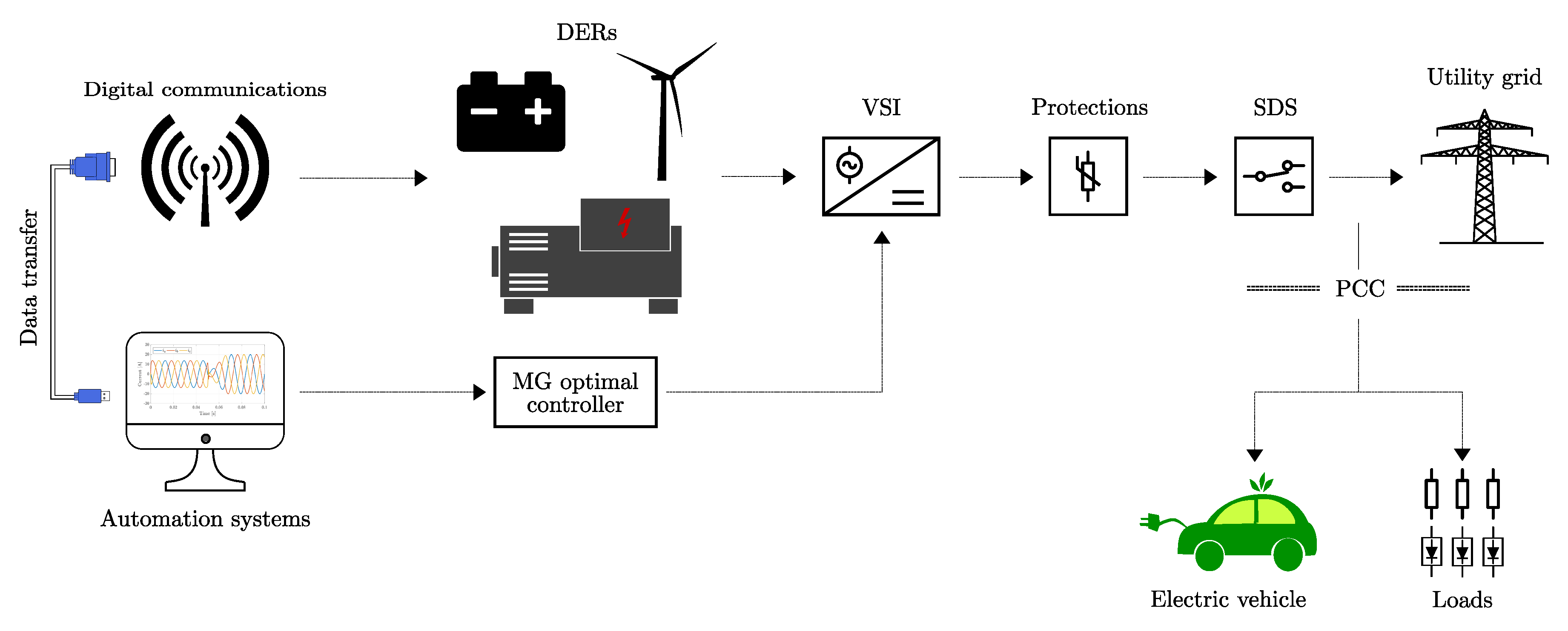
Figure 1 shows the essential components that integrate an MG. The MGs are defined as the small local distribution systems which promote the use of DERs. DERs are small energy units of generation and storage. These can come from renewable energy sources such as wind turbines, non-renewable energy sources such as diesel generators, or energy storage systems such as batteries. It has linear loads, non-linear loads, or dynamic loads such as electric vehicles. The MG operates in grid-tied mode or stand-alone mode. To achieve this, it has protections and control systems that allow connection and disconnection to the utility grid safely and without affecting its stability. Energy management is established through measurement and control systems. These systems allow the MG to operate with a decentralized or centralized control scheme, which has a direct impact on the MG’s power quality and reliability. While MG operates in grid-tied mode, unbalanced loads or grid failures are originated by unbalanced currents and voltage at the Point of Common Coupling (PCC) affecting the energy quality index [
6,
7]. In our study, the SDS located at the PCC is assumed as closed. Hence, the MG is operating in grid-tied mode.
Likewise, MG voltage depends on the connections associated with the electric grid. Thus, unbalanced loads connected at the PCC provoke that the Current Source Inverter (CSI) may supply three-phase unbalanced currents with components of a negative-sequence directly towards the MG. This effect degrades the CSI performance and the energy quality index due to fluctuations in the inverter’s current and power signals. In this way, negative-sequence components are generated in the measured current at the PCC, affecting the current balance percentage, ruled in the IEEE 1159-1995 standard [
8]. Moreover, nonlinear loads introduce a band of harmonics into the MG, producing distorted waveforms at the current signal in the utility grid and CSI output. MG must attenuate such harmonics to avoid include perturbations on the system dynamics, as well as in the sensitive loads connected simultaneously at the PCC.
On the other hand, control approaches on MGs are focused on separating current and voltage signals from the negative and positive sequences in the CSI to address these electrical grid issues [
7,
9,
10]. Obtained such a decomposition, a control law is designed for each of these components to increase the CSI control performance [
11]. Several studies have proposed to improve the energy quality index by reducing the negative-sequence component of the control signals [
12]. Dasgupta et al. worked on a current controller based on the Lyapunov function to control the active and reactive power flow to a three-phase MG system [
13]. The Fault Current Limiter (FLC) is another methodology that suppresses fault currents from the utility grid, assuring the good operation of the MG. This tool seems to solve the over-current relay coordination issue in the MG [
14]. Surrender et al. proposed a collaborative optimization framework, including the Differential Evolution (DE) and Harmony Search (HS) methods, to obtain the efficient energy resources distribution in the MG. The MG was composed of several renewable energy sources where the optimization processes involved energetic, economic, and environmental factors [
15]. Lotfollahzade et al. used an LQR-PID controller optimized by PSO (Particle Swarm Optimization) to compute the proportional, integral, and derivative parameters to obtain an optimal load sharing of an electrical grid [
16]. Savage et al. proposed to design hierarchical control techniques to enhance the energy quality in the connected bus at sensitive loads [
17]. A primary control took DERs administration, and secondary control drove the voltage levels at the load bus by sending the control signals to the primary block for compensating the unbalances. Shi et al. tested a control strategy under three-phase unbalanced [
10]. They proposed a unified three-phase voltage correction through negative-sequence compensation. In practice, dynamic systems need to use robust, versatile, and tunable control strategies, in that sense, the hybrid control is becoming a reliable alternative in automatic systems, especially in MG. Lindiya et al. adopt a conventional multi-variable PID and LQR algorithm in DC-to-DC converters for reducing cross-regulation [
18]. For realistic simulation of MG performance, Momoh and Reddy present a platform to simulate basic MG using Hardware-In-Loop (HIL) under different environments [
19]. This interesting tool allows testing divers controllers and measures the performance of the MG on delivering the power supply requirements under different scenarios.
In other related areas, Sen et al. tuned a hybrid LQR-PID controller to regulate and monitor the locomotion of a quadruped robot using the Grey-Wolf Optimizer (GWO) [
20]. Besides, Nagarkar et al. proposed a PID and LQR control to optimize a nonlinear quarter car suspension system [
21]. Ibrahim et al. integrate the dynamic behavior of an LQR-based PID controller applied to a helicopter control with three degrees of freedom [
22]. In this article, an efficient control technique based on PI-LQR driven by a Genetic Algorithm (GA) and a high-accuracy fitness function is proposed to regulate the energy provided by an MR. A genetic algorithm warranties that LQR is behaving according to design requirements as settling time and overshoot of the transfer function modeling the MG. To reach the appropriate current and power values to be supplied by the MG, a PI control strategy is included in the optimized transfer function. In such a sense, the required characteristics are a low-cost operation of the system during LQR operation, and the error reduction in the steady-state while using the PI control.
Consequently, an LQR-PI control technique is proposed to conduct the control action of the CSI, so the operation can operate in the negative-sequence mode. Besides, this action helps to mitigate the negative-sequence components of the current signal injected by the MG, phenomena caused by unbalanced linear and nonlinear loads. On the other hand, the proposed control methodology reduces the harmonic distortion generated by nonlinear loads, which is computed by the Total Harmonic Distortion (THD). Moreover, such schemes guarantee the current equilibrium at the PCC, and an acceptable energy quality index according to the norm ruling the MGs. The significant contributions of this paper are to propose the GA with an effective and accurate fitness function that helps to calculate the controller design parameters and to hybridize the properties of PI and LQR controllers applied to the MG to provide the demands of energy. This methodology looks for improving quality energy issues considering the energetic cost of the system during its operation and compares the classical methods used to design PI controllers applied to MG.
2. Microgrid Structure Analysis
The MG configuration used in this work is shown in
Figure 2.
The utility grid is represented by a three-phase voltage source and its coupling impedance. The linear and nonlinear loads are connected at the common coupling point. In particular, linear loads have a three-phase configuration and operate with a unity power factor. Contrarily, nonlinear loads are modeled as controlled, single-phase current sources. This scheme allows controlling the harmonic content in each of the phases of the MG. Besides, the MG is connected to the PCC employing an SDS switch that is kept closed to operate in a grid-tied mode. Electrically, the MG is represented by an equivalent circuit consisting of a Renewable Energy Source (RES), a converter and a low-pass filter. An ideal voltage source serves to represent the RES because of its energy is directly taken from clean photovoltaic cells. Moreover, there are no associated mechanical components of inertia as in microturbines, wind turbines, among others [
23]. The converter is in charge of performing the power transfer between the DC bus and the AC network. An LCL low-pass filter is required to attenuate the currents’ high-frequency components provided by the MG (
,
,
).
LCL filters have great advantages considering aspects as a reduced cost and size because the estimated values of the inductors are smaller than L and LC filters topology [
24]. Besides, this efficient filter shows better performance on filtering high-frequency harmonics generated by the switching of PWM converters, including grid-connected converters controlled by the current sources [
25]. In our study, the SDS that links the MG with the utility grid is considered closed because of MG is operated in grid-tied mode. This analysis considers that the MG provides active power to supply energy into the loads connected to the PCC. In case of failure or instability in the utility grid, the MG works as a support system injecting or consuming reactive power to balance the voltage at PCC. For such a purpose, the methodology seeks to control the currents by a set of inductors located just aside the PCC, considering that these elements deliver the power toward the utility grid directly.
In practice, the Park transformation is used for obtaining a simplified state-space model of the MG to dispose of a decoupled system representing the MG behavior [
26]. First, the passive elements (inductors and capacitors) are considered to have the same value for each of the phases. Therefore, the three-phase representation of passive elements is given by
where
is the identity matrix of order 3,
and
are the passive components’ scalar values in each phase. Second, a framework mapping from the three-phase
to the
domain is applied to the passive elements. Such a mapping is made by the well-known current-tension relations for inductors and capacitors as follows,
Third, the Park transform
is then applied to Equations (
2) and (
3) to obtain an orthogonal rotating reference frame (
).
where
represents the axes turning-speed for a determined phase, and in the mapping framework,
is defined by
. Thus,
operator is well-known as the Park transformation. Finally, Equations (
4) and (
5) are solved using the chain rule with
=
to achieve the
model for each passive element,
These foundations are mathematically represented by the state-space model given in Equations (
10) and (
11)
where
and
represent the
components of the input voltage source. The functions
and
are used to include the system response face to perturbations, which are modeled by Equations (
12) and (
13),
where the active variables
and
represent the
components of the electrical grid signals. Such perturbations affect the system behavior meaningfully and whose effects must be reduced or eliminated. Indeed, our model is based on the state-space using the Park transformation to simplify the MG analysis so that it is possible to obtain two decoupled systems in the
framework [
27]. The
d component controls the active power flow, whereas the
q component regulates the reactive power flow, respectively.
All MG interactions are formally described in the state-space system represented by Equations (
10)–(
13). In such a representation,
,
,
,
,
, and
are the voltages in the inductors
and
, as well as the current in the capacitor
into the
framework, respectively. Similarly,
,
,
,
are the inductor currents and
,
are the capacitor voltages in the
reference frame. After estimating the system response, the results allow determining that the modeled MG is critically damped because the transfer function that describes the dynamic system has two complex-conjugated poles on the imaginary axis. In consequence, the method of states-feedback is applied to dispose of a more suitable allocation of the system poles, which will improve the response to the step input. New control law representation and the derived dynamics system are described by Equations (
14) and (
15)
where
is the system input,
is system reference, and
K represents the state feedback gains. The state vector can be calculated by the dominant pole placement technique, which consists of matching the system characteristic polynomial with a theoretical polynomial containing all needed control parameters (i.e., overshoot, rise time, settling time, among others). However, this technique presents a problem tied to the arbitrary pole assignment, which directly affects the control effort with inconvenient or impractical values in the gain matrix
K. Therefore, the LQR algorithm was implemented and evaluated to address previous shortcomings in the analysis of the MG. The
K matrix is then optimally computed to find the best poles placement of the system [
28]. The full state feedback control allows a suitable selection of the components describing the dynamics of the systems [
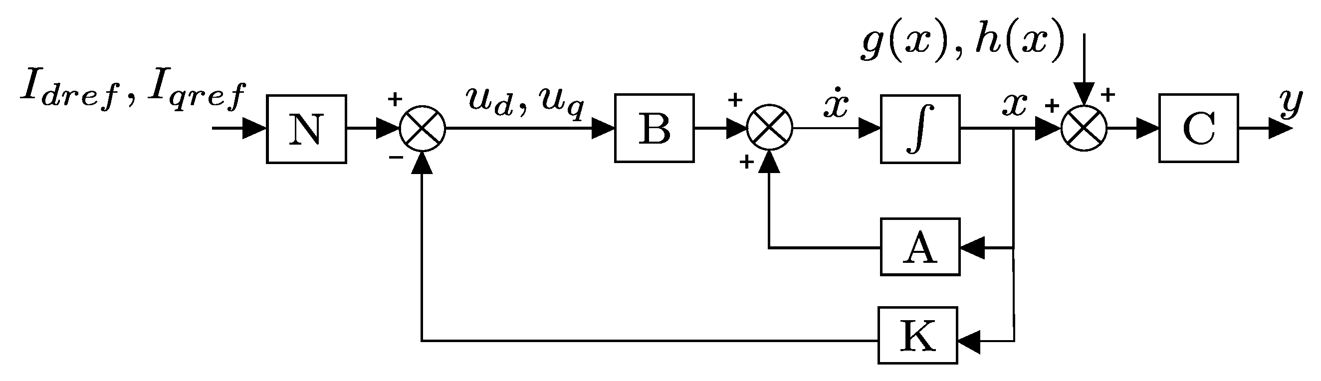
29], in this case focused on controlling the MG where the design is driven by GA. The proposed diagram of full state feedback is shown in
Figure 3.
In the diagram, matrices
are the original system matrices in the state-space representation given by Equations (
10) and (
11),
K is the state feedback matrix, and the precompensation gain
N is a scaling factor that multiplies the system reference to achieve the output desired value
. Indeed, the
N scaling factor is calculated by
Additionally, the cost function required by the LQR algorithm to obtain the optimal control parameters is defined as follows,
where
,
are positive semi-definite matrices.
Q is the state matrix penalization, and
R expresses the actuator effort. The cost function
J is subject to the next system constraint,
where
and the
are vectors ∈
. Thus, the original system input and state vector are theoretically calculated by
The LQR optimization problem requires firstly to solve the algebraic Riccati equation,
In some cases, the matrices
Q and
R could be assigned arbitrarily; unfortunately, the control design over the required system response could be compromised or impractical. Hopefully, to address those disadvantages, the Riccati equation allows assigning state penalization values that belong to matrix
Q and
R to modify the speed response of the LQR controller. Therefore, it is possible to compute the values of the matrix
K and the system input
by solving
S of Equation (
21). However, when faster and more efficient system dynamics are required, the random parameters assignation in the matrix
Q and
R can lead to a second problem. In that case, the estimated values of matrices
Q and
R grow out of the allowed range to fulfill the control design requirements (e.g., settling time and overshoot) of the transfer function describing the MG. This issue is efficiently addressed by using an optimization method to compute the matrices
Q and
R. Hence, a proper cost function, involving the overall design requirements of the transfer function jointly with the parameters of the LQR algorithm, is then minimized. For overcoming the issues of arbitrary pole placement, a genetic optimization algorithm was also proposed in this study, since this optimization technique can operate in parallel to find multiobjective solutions [
30].
3. Genetic Algorithms
The genetic algorithms (GA) are metaheuristic algorithms belonging to the family of evolutionary algorithms (EA). All population-based algorithms work with a set of candidate solutions called phenotypes or population and a set of chromosomes representing the model’s variables. Each candidate solution in the population is coded in a chain of chromosomes or genotypes. Since these algorithms are inspired in the natural selection, the chromosomes evolve throughout each iteration (i.e., generation) to produce new individuals (i.e., solutions). In each generation, the best chromosomes or individuals are selected by evaluating a suitable fitness function. The next generations are generated by applying a fundamental set of genetic operators until achieving the optimal result. The traditional chain of genetic operators comprises the initialization, crossover, mutation, and selection, as is shown in
Figure 4.
A new generation is processed when the requirements of a stop condition are not fulfilled [
31]. A GA implementation could present many variations, which depends on the particular way of how each genetic operator is applied. The methodology driven by the GA to solve the energy cost issues based on the LQR controller is described by Algorithm 1.
| Algorithm 1: Genetic Algorithm. |
| 1. Generate a random initial population. |
| 2. Evaluation of each individual in the fitness function. |
| 3. Verify the Stop criteria to detect the optimal solution. |
| 4. Selection or Elitism of the best individuals that will be crossed into the crossover function. |
| 5. Crossing the selected individuals (interbreeding) to generate new progenies or solutions. |
| 6. Mutation of random chromosomes in each individual to diversify the searching space. |
| 7. Applied the genetic operators, the best individuals must repopulate the next generation. |
| 8. The optimal solution is found fulfilling the stopping criteria, otherwise, continue Step 4 |
The GA starts with a random assignation of the chromosomes in each individual representing the variables of the proposed models. In this manner, each individual is a viable solution that must be further evaluated, and the overall initial individuals will form the initial population. In our implementation, the chromosomes represent the values of each element into the matrices Q and R as described next.
3.1. Chromosome Configuration
The proposed control modeled in real continuous variables led to select a floating-point representation of the chromosomes. In this case, bit string encoding mechanisms can be replaced for floating-point operations in the mutation and crossover functions. The chromosomes represent each variable to identify in the proposed control. In the proposed implementation, four chromosomes were used, three elements to describe the Q matrix, and one element for the variable R that internally are linked to the gains and poles in the system. It is noteworthy that such elements describe the control behavior while interacts with the MG. This controlling behavior is measured at the output by well-known design parameters (e.g., overshoot, settling time, undershot, stable error, rising time, or natural frequency). In the numerical simulations, settling time and overshoot factor were used in the fitness function. Hence, the chromosomes were coded in floating point, as well as the uniform distributions were used to control the action of the morphological operators acting over chromosomes randomly selected. The initial population was fixed to N = 100.
3.2. Mutation and Crossover
Before mutation, the best suitable solutions (elite population) are selected and preserved. The elite population comprises the 5% of the total population, saving the fittest genetic material. The mutation operator using a floating-point representation is defined by
where
,
is the chromosome randomly selected from the entire database
X, which is mutated by a bounded interval
, and
is a random number with uniform distribution
. Hence, the algorithm was tuned to generate 20% of new chromosomes
. The mutation should produce new individuals with a probability of about 20% in our implementation. The crossover function used an unbalanced arithmetic operation defined mathematically as
where
is a random number uniformly distributed
,
is randomly selected between the best 25% of individuals and
is randomly selected from last 75% in the prevailing population. Considering the elitism preserved 5% of the population, and the mutation provided 20%, the crossing probability could be about 75%.
The crossover and mutation probabilities are eventually modified depending on the individuals’ fitness to achieve a good trade-off between exploration and exploitation. In fact, the mutation and crossover probabilities should slightly increase when the population is trapped into local optima, and such probabilities decrease when the population is too dispersed. In the order hand, there is no general consensus on how to measure and balance the exploration and exploitation efficiently in genetic algorithms [
32]. In our implementation, this trade-off involves direct parameters of the algorithm, the number of generation and the population size, combined with the population diversity controlled by the crossover, mutation, and selection functions. Mutation and crossing explore a new solution with a conjoint probability of
, and the exploitation uses basically the elitism function
, which express certain skew to the exploration in our implementation.
Finally, the GA selects the optimal solution for each chromosome (i.e., optimal matrices Q and R) by using the appropriate cost function and the LQR algorithm, to achieve the desired behavior of the system.
3.3. Fitness Function
The fitness function is related to the error between the actual solution and the optimal solution, represented by the controlled MG behavior (i.e., overshoot and settling time) associated internally to the best chromosomes in the
Q y
R matrices. In control terms, the fitness function is related to signal error between the output and the set-point responses. However, computationally some parametric error could be used as Mean Absolute Error (MAE), Mean Squared Error (MSE), Mean Absolute Scaled Error (MASE), among others. The commonly used MSE merit function is highly affected by outliers, which produces undesirable results in some applications, such is the case of the proposed design. Therefore, the MAE function was used to cope with this disadvantage obtaining satisfactory results in the implemented GA algorithm. The MAE based on the
-norm is mathematically defined as
where
is the actual value and
is the estimated behavior vector response of the proposed controlled model. This modest fitness function is really dependent on highly nonlinear parameters of the control interconnecting the grid, loads, and the power sources, which can be dynamically adjusted with the proposed GA optimization algorithm. Including the output control parameters of interest, the fitness function becomes,
where the vector
contains the desired parameters as the settling time (
) and the overshoot
, and
W is a regularization (or scale) matrix to adjust the contribution and units of each kind of parameters. Besides,
is the system’s response parameters under the control action, while the chromosomes representing the control operational matrices
Q and
R. The data used by the fitness function is computing by solving the dynamical model used to represent the control and the MG for each individual in the population. The weight matrix is defined as
where
are the constants allowing to prioritize some of these output features,
, and
are the maximum or actual values of the tested features to avoid dimensionality issues. The chosen fitness function is highly stable for the proposed model. It is worthy to notice that optimal
Q and
R matrices are highly dependent on the chosen fitness function, which could also be interpreted as an error function.
4. LQR-PI Control Strategy for MG in Grid-Tied Mode
Once computed the matrix
K driven by GA, the PI-LQR controller is designed to regulate the power flow from MG toward the utility grid. A robust and performing controller is obtained by combining the optimal properties of the LQR algorithm and a classical PI controller. Such a strategy allows achieving a bounded control action.
Figure 5 illustrates the control action for the MG output voltages either to the hybrid PI-LQR controller, PI controller driven by GA, or PI controller tuned by the poles placement method. Control action values are into established parameters by MG voltage.
It is noticeable that the control action helps the system to recover and operate under established values for MG voltage (see Table 2). This signal controls the three-phases of the CSI switching-pattern to deliver the required power at the electrical grid. By the way, the controller’s integral action also reduces the sensitivity face to perturbations, canceling the steady-state error for unit step inputs [
33]. The PI control action is mathematically described by
where
and
are the proportional and integral gains, respectively. All these gains were calculated by using the rlocus method, considering the suitable phase and magnitude conditions into the controller design.
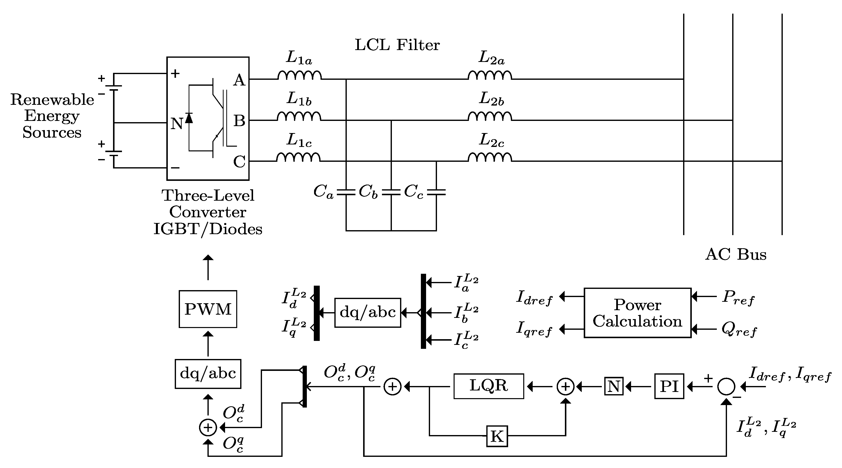
Figure 6 shows the optimal control scheme used to regulate the power flow at the PCC.
The instantaneous
power theory is used to adjust the input references of the control system in the model shown in
Figure 6. Such theory is based on a set of instantaneous powers defined in a temporal framework that imposes no constraints on the voltage or current waveforms. Thus, the same approach can be applied to three-phase systems with or without neutral wire [
26]. In the proposed solution, the Park transform should be applied to convert the state-system from a three-phase framework (sinusoidal variables) to the
orthogonal reference system (constant values). Park transform allows synthesizing and decoupling the variables and associated states forming the MG. In this sense, the input references’ values are obtained using the
theory and Park transformation by
Thus, the control signals are transformed into the three-phase frameworks for regulating the PWM signals into the three-level converters. Since PWM signals control the switching sequence of CSI, the model produces the desired power that the MG must inject toward the utility grid.
5. Energy Quality Index Applied to the Current Signal at the PCC
Low voltage systems include linear and nonlinear single-phase, two-phase, and three-phase loads. These loads cause the system to become unbalanced, and consequently, the current and voltage waveforms of three-phase sources are not identical in magnitude and phase. Unfortunately, some electrical machines depend on a balanced power supply to avoid affectation on their functionality and performance [
34]. When the MG operates in grid-tied mode, the failure generally comes from the utility grid and unbalanced loads resulting in three-phase unbalanced voltage at the PCC. However, the unbalanced factor could be quantified in a three-phase unbalanced system by using the symmetrical sequences approach. Such a method decomposes the unbalanced system into three sequence components, called the positive, negative, and homopolar sequences. This unbalanced percentage is calculated by the ratio of the negative and positive-sequences, which is formally known as voltage unbalance factor (
VUF) and defined by Equation (
30),
where
and
are the negative and positive sequence components, respectively; both voltages are measured at the PCC. Similarly, the definition of
VUF could be adopted to measure the current unbalance factor
CUF, which is given by
where
and
are the negative and positive sequence components, respectively; both currents are measured at the PCC. The currents
are measured at the inductor bank
of the MG through the sequence analyzer, where
. Our approach uses
CUF because the designed control strategy is based on a current control loop. Thus, the CUF index is computed with the current signals provided by the MG at the PCC. Otherwise, linear, and nonlinear unbalanced loads may produce excessive levels of unbalanced current and voltages that tend to appear in the MG. These phenomena’ main effects are lower performance, energy losses, and instability of the MG [
35]. In the presence of negative-sequence components, the power electronics converters and induction motors cannot work or perform poorly [
36]. An unbalanced voltage can produce an unbalanced current from 6 to 10 times the magnitude of the unbalanced voltages. Unbalanced currents can provoke excessive heat in the motor windings, leading to permanent damage [
37]. The IEEE 1159-2009 standard establishes that the current unbalance recommended for monitoring power electronics, in steady-state, should be between 1% and 30% [
8].
Another phenomenon affecting MG behavior is the increased use of nonlinear power electronic devices and sensitive loads [
38]. These devices induce harmonics that may degrade the components either in the utility grid or MG. High-frequency harmonics can be filtered by passive or active filters, but the low-frequency harmonics are difficult to filter without reducing the system’s operating frequency. There exist methods to mitigate the low-frequency harmonics, but these techniques are expensive and difficult to implement [
39]. The current or voltage distortion is measured through Total Harmonic Distortion (THD), such index is applied to the voltage or current as follows,
THD is defined as the ratio of all root-sum-square of all harmonics (excluding the fundamental) divided by the fundamental [
40]. The typical limit used in low-tension is about 5% of THD. In this study, the THD index is applied over the current signal delivered by the MG to evaluate the control performance face to harmonics generated by unbalanced nonlinear loads connected at the PCC.
6. MG Control System Design
Three optimal controllers were designed and analyzed to obtain the best response considering criteria as low-cost energy, mitigation of negative-sequence, and harmonics reduction. Low-cost energy criterion is directly associated either with the input source voltage or with MG voltage. In other words, such value expresses the energy required by the system to execute the control action over the injected current by MG, considering the respective estimations of Q and R matrices, the state feedback matrix K, and the control PI parameters and . For each one of the designed controllers, three study cases were set up to evaluate the performance of the control schemes, which fulfilled the design criteria given initially. Proposed three study cases are based on making MG operate under the next conditions:
MG faces balanced nonlinear loads, the harmonics and negative sequence attenuation are analyzed.
MG works under unbalanced nonlinear loads, the harmonics and negative sequence mitigations are studied.
MG handles the unbalanced linear and nonlinear loads simultaneously; the attenuation of harmonics and negative sequence are both quantified.
The LQR algorithm is used to estimate the gains of feedback states driven by the GA method. Likewise, a PI controller was tuned to reach a robust control technique designed in all study cases. The design parameters of the LQR controller include a settling time, = 0.525 ms, and an overshoot of 5%. For simulation purposes, the MATLAB/Simulink environment was used to evaluate the proposed MG control system.
6.1. Hybrid PI-LQR Control Driven by GA
GA implementation starts tuning the initial values of all chromosomes. Each chromosome represents a potential solution to the weights of matrices
Q and
R, which eventually adjust the controller’s desired behavior. In the proposed model, the fitness function (see
Section 3.3) performs the quality measure or associated error to each set of chromosomes representing each potential solution. The LCL filter parameters are given in Table 2. Such parameters are constant for all study cases and represented in the state space system given in Equations (
10) and (
11). The control parameters obtained from LQR driven by the GA, are estimated by,
Besides determining
Q and
K matrices, the pre-compensation gain
N = 408.5786 and parameter R = 0.0518 were also estimated. Those values were simulated in the proposed model to achieve an output settling time
= 0.52454 ms and an overshoot of 4.4643%. The parameters utilized by GA for tuning the established criteria of the LQR algorithm are summarized in
Table 1.
After tuning the parameters of the LQR method, the
and
PI controller parameters are determined through the rlocus method. A contribution of this study is to combine two control design methodologies to propose a hybrid PI-LQR controller, whose performance was tested on the MG model using Simulink. The utility grid is represented in the simulation model by its Thevenin equivalent (i.e., a three-phase electric source and the coupling impedance). The MG is integrated by a passive filter with topology L-C-L (Inductor-Capacitor-Inductor), a three-phase inverter based on IGBT technology controlled by the current loops (
and
), and the DC bus, which is powered by a voltage source. For all study cases, the current references for
components were set at
A and
. MG simulation parameters for the hybrid PI-LQR controller are shown in
Table 2.
Figure 7 shows the numerical results corresponding to the MG operation under the action of either (1) the hybrid PI-LQR controller, (2) the PI controller driven by GA, or (3) the PI controller designed by the poles placement technique, under the same operating conditions (linear balanced loads).
The graphical responses of such controllers are equivalent. It is noteworthy that the controller is intentionally inactive in the initial interval of time,
s, to have a reference for checking the posterior control action, as shown in
Figure 7. The current flows from the utility grid towards MG during this time interval, so the MG is consuming power. The controller starts to operate since
t = 0.05 s, which produces a transitory response ending at
t = 0.066 s. In this period, the MG current reaches the reference current (
= 20 A and
= 0 A).
Moreover, the MG tracks the set-point until the desired current amplitude is injected into the system (
= 20A,
= 20 A, and
= 20 A). The system was analyzed under ideal balanced conditions, including linear loads from simulated starts. This test is a start-up test of the hybrid PI-LQR controller working under normal operating conditions to demonstrate the method’s correct operation. The same simulation is used for all study cases regarding the times of activation and deactivation of the hybrid PI-LQR controller.
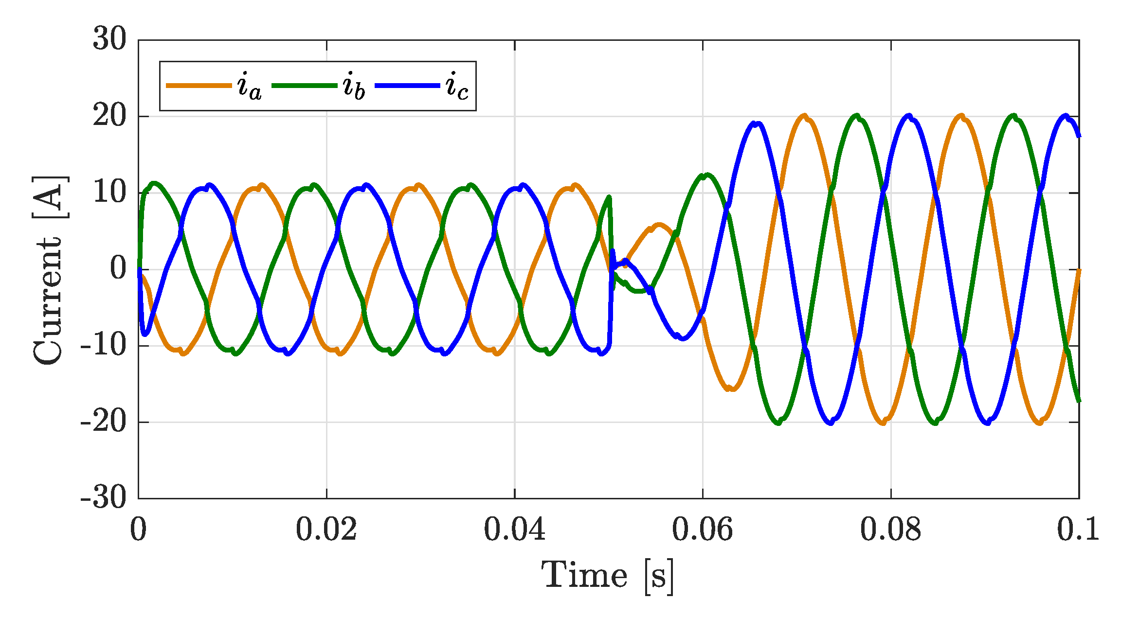
Figure 8 shows the performance of the action of either hybrid PI-LQR controller, PI controller driven by GA, or PI controller by poles placement under the presence of unbalanced linear loads.
Considering the same operating conditions and equivalent control responses because of the differences of such controllers are studied, respect the energetic cost, negative sequence mitigation, and harmonics attenuation. Remarkably, a CUF index of 9% was reached when the controllers are disabled, but a CUF index of 1% is obtained when the controllers are under operation for unbalanced linear loads. The MG behavior is evaluated by connecting balanced nonlinear loads at the PCC to test control robustness. The nonlinear loads implemented in the simulations consist of three single-phase uncontrolled rectifiers. For such a case, the magnitude of the harmonics is calculated by
, where
is the current of the fundamental component for each phase, and
is the harmonic order.
Figure 9 shows the current correction of the distorted current waveform, which was affected by operating under balanced nonlinear conditions. The amplitudes of the fundamental nonlinear load currents are
A,
A, and
A for the balanced case.
Additionally, an FFT analysis was applied to obtain the spectral component of the current signal for studying the THD
index behavior for each phase. From this analysis, the THD(
) = 5.08%, THD(
) = 5.08%, and THD(
) = 5.08% indexes are obtained when the controller is disabled. Contrarily, the THD(
) = 2.51%, THD(
) = 2.51%, and THD(
) = 2.51% indexes are reached when the hybrid PI-LQR control is activated. Besides, the harmonics of the 5th and 7th order are substantially attenuated for balanced nonlinear loads; such results are included in the second and third columns in
Table 3.
In the same context, a study case concerning an unbalanced nonlinear load was analyzed to test the MG performance. Here, the amplitudes of the fundamental unbalanced nonlinear load currents are given by A, A, and A.
In the simulation, the CUF produced by the unbalanced nonlinear loads preserves the CUF ratio considered in the unbalanced linear load’s study case.
Figure 10 shows the distorted waveforms belonging to the current signals that lost the original sinusoidal shape under the effect of nonlinear loads.
However, activated the hybrid PI-LQR controller, the current signal is gradually improved and balanced by the action of the MG control. The CUF index produced by the unbalanced nonlinear loads was 11%, but by using the hybrid control, this index was improved to 1%. Similarly, a harmonics study was implemented to analyze the effects of unbalanced nonlinear loads over the current signal injected by MG.
Table 3 (four and five columns) shows the harmonics reduction behavior under unbalanced nonlinear loads, which leads to reduce the THD(
), THD(
), THD(
) indexes from 5.47%, 11.83%, and 18.39% to 2.49%, 4.63%, and 4.61%, respectively.
Finally, the case of unbalanced linear and nonlinear loads connected simultaneously at the PCC is studied.
Figure 11 presents the result of the hybrid PI-LQR controller operation under the actions of both loads.
In this case, a high CUF = 18% index is obtained while the control is deactivated. Once the controller is activated, the CUF is reduced to 2%. As in the unbalanced nonlinear load case, a significant reduction of harmonics was obtained, and the results are included in
Table 3 (six and seven columns). THD indexes (
and
) were reduced from 4.39%, 9.15% and 14.31% to 2.11%, 3.39% and 2.97% for this study case.
6.2. PI Controller Driven by GA and Rlocus Design
The GA was implemented for tuning the matrix
K in the rlocus method (poles placement method). In this case, only one chromosome (
) was used together with the design parameters as the undamped natural frequency (
), settling time (
), damping factor (
), and overshoot (
) to calculate the components of
K. Therefore, the matrix
K could be estimated by
where
represents how far the third pole is located according to the dominant poles configuration [
41]. The fitness function to determine the matrix
K, considering the design parameters, is defined as
where MO
is the maximum allowed overshot, and O
is the actual overshot. The control parameters
and the precompensation gain
N = 1845.7 were estimated using this genetic approach. The compensated system achieved a settling time of
= 0.5593 ms and an overshoot of 4.9109%.
Table 4 summarizes the parameters used in the GA for tuning the poles placement method.
Finished the tuning process, the PI controller is designed through the poles placement method, and the simulation tests are then analyzed. The simulation parameters are given in
Table 5.
The simulation results were carried out on a set of interconnected nonlinear loads, which allowed testing the PI controller response under balanced and unbalanced nonlinear conditions.
Figure 12 presents the PI controller performance driven by GA.
The control was able to compensate for the current distorted waveform, produced by balanced nonlinear loads. This methodology reduced the THD(
), THD(
), THD(
) indexes from 5.26%, 5.26% and 5.26% to 1.35%, 1.35% and 1.35%. Likewise, the harmonic content reduction is shown in
Table 6 (two and three columns) for this study case.
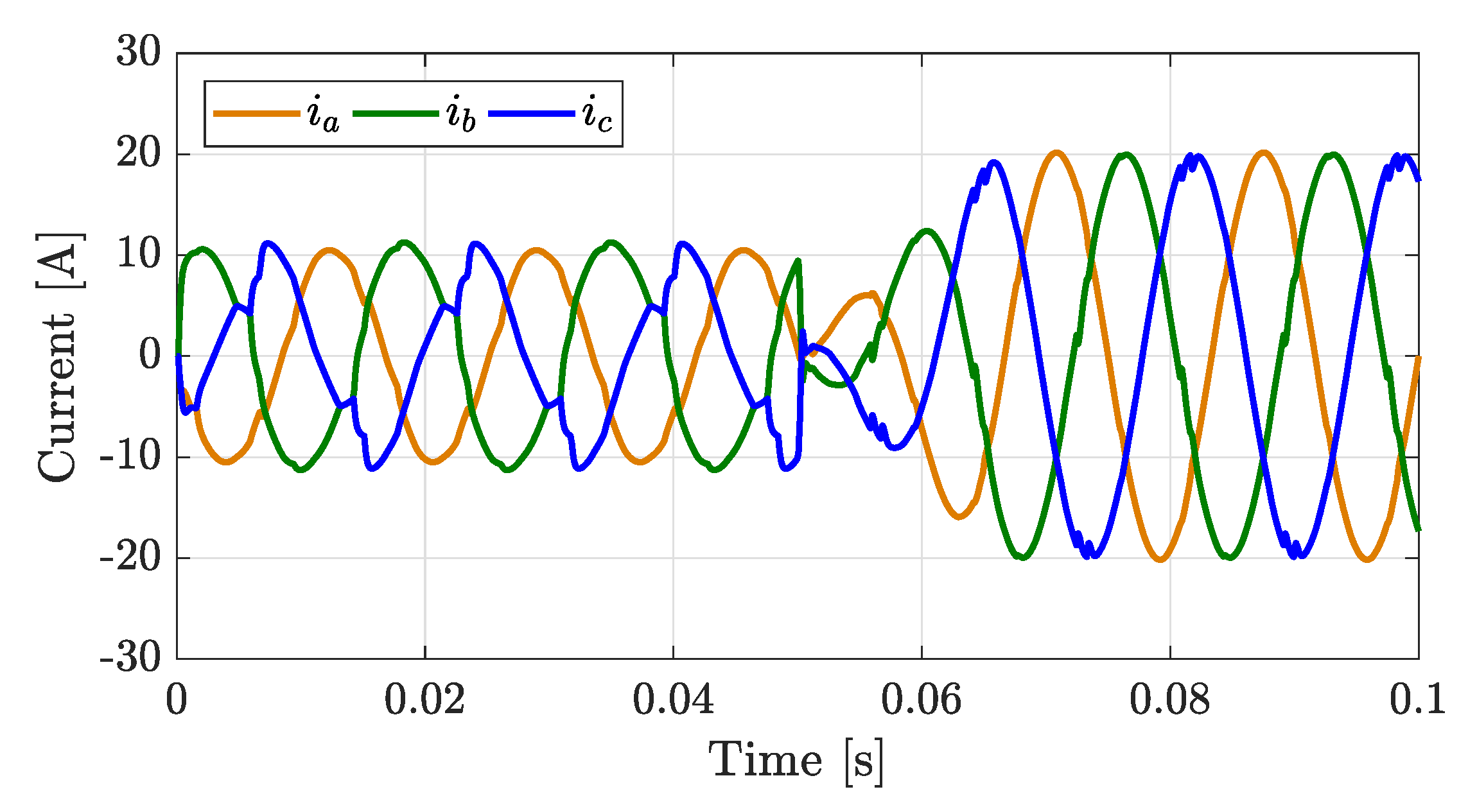
Figure 13 shows a study case considering unbalanced nonlinear loads to verify the control quality face to harmonics and unbalanced actions of the MG control.
The numerical results generated a CUF = 11% for unbalanced nonlinear loads, but the index is reduced to 0.6% once the controller is activated. Similarly, the THD(
), THD(
), and THD(
) indexes of the current signals injected by MG are reduced from 5.61%, 12.09%, and 18.69% to 1.30%, 2.50%, and 2.55%, respectively. In
Table 6 (four and five columns), the harmonic content reduction corresponding to this study case is shown. In
Figure 14, unbalanced linear and nonlinear loads were connected and simulated, which gave an improved performance for an unbalanced current compensation from 18% to 2%.
The harmonics were significantly reduced, which is depicted in
Table 6 (six and seven columns). Likewise, a THD reduction was carried out, attenuating the THD(
), THD(
) and THD(
) indexes from 4.56%, 9.34%, and 14.53% to 1.14%, 1.73%, and 1.53%, respectively.
6.3. PI Control Design by the Poles Placement Method
In this design, the LQR algorithm was implemented to estimate the
K matrix of feedback states. Besides, the penalization matrix
Q and effort control
R were assigned according to the requirements initially established using the poles placement method. The LQR control matrices and parameters assigned by the designer were determined as R=0.002 and pre-compensation gain N=707.9018,
Numerical results gave a settling time
= 0.525 ms and an overshoot = 6.39%. Next, the PI controller’s
and
constants were calculated, combining the properties of LQR and PI controllers. The simulation parameters for this case study are shown in
Table 7.
Similarly to the last two controllers, the MG behavior under balanced nonlinear loads, unbalanced nonlinear loads, and unbalanced linear and nonlinear loads connected at PCC was analyzed.
Figure 15 shows the controller performance under balanced nonlinear conditions, reducing the THD(
), THD(
) and THD(
) indexes from 5.27%, 5.27% and 5.27% to 2.30%, 2.30% and 2.30% respectively. Harmonic reduction through PI controller by dominant poles is shown in
Table 8 (two and three columns).
In the presence of unbalanced nonlinear loads, a CUF = 11% index is initially obtained, but those indexes are significantly reduced to 1% under the MG control. Such an effect is shown in
Figure 16.
In the same sense, a considerable harmonics mitigation was induced, which is given in
Table 8 (four and five columns). Additionally, THD indexes of three phases were attenuated from 5.60%, 12.05%, and 18.65% to 2.27%, 4.22%, and 4.22% for this study case.
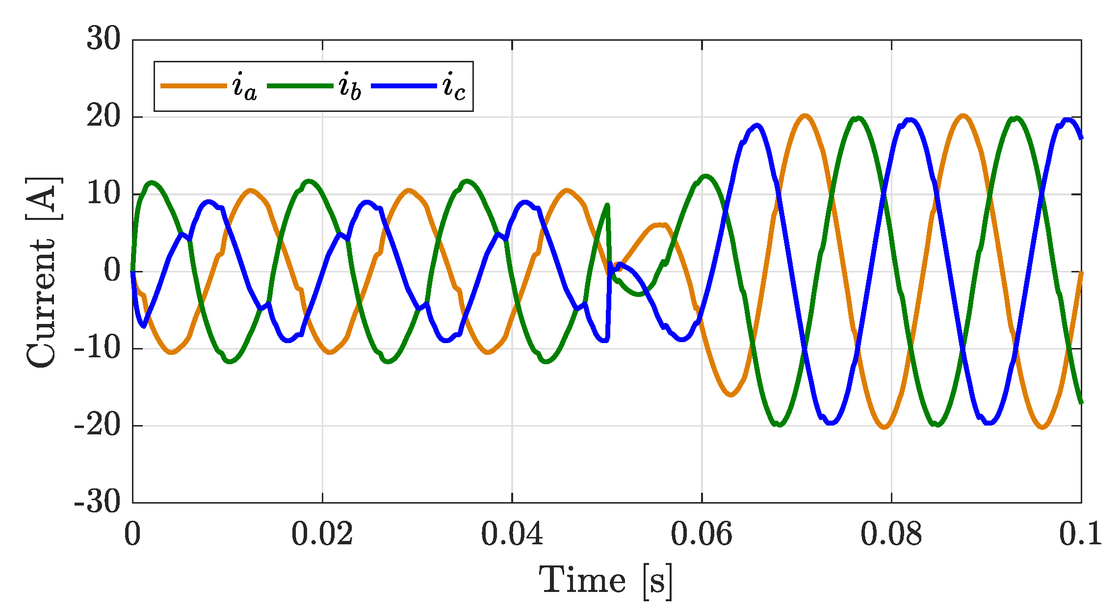
Figure 17 shows an unbalanced linear and nonlinear study case to verify the controller performance.
Under these conditions, the numerical results determine that MG reduced the current unbalanced index
from 18% to 2%. The respective harmonic reduction is shown in
Table 8 (six and seven columns). Besides, THD indexes (
,
, and
) were reduced from 4.53%, 9.30%, and 14.30% to 1.94%, 3.08%, and 2.68%, respectively.
It is noteworthy that the harmonic content shown in
Table 9 is extracted from the harmonic content from
Table 3,
Table 6 and
Table 8 when the controller in operation (see columns 3, 5, and 7). The energetic cost is associated with the MG Voltage (V
) parameter highlighted in Line 2 from
Table 2,
Table 5 and
Table 7. Numerical results in
Table 9 allows determining that PI controller driven by GA obtained the best THD
factor for the three study cases. Nevertheless, to reach this low distortion was necessary to use the higher DC voltage (i.e., 1000 V), which could be highly restrictive and expensive in practice. On the other hand, the hybrid LQR-PI reached the lower energetic cost consuming only 311 V
. Additionally, the measured harmonic distortion under this control action fulfills the allowed THD limits of 5% and is pretty close to the best results given by the PI controller driver by GA. Finally, the positive impact of saving energy by using the hybrid LQR-PI is fundamental in the selection criteria in an efficient MG system.
Finally,
Table 10 shows the comparison between research works found in literature and the proposed approach using related hybrid PI-LQR controllers.
This study proposed an efficient optimal control technique, combining the performance of LQR and PI controllers tuned by Genetic Algorithms using a reliable fitness function. The particular discriminant definition of the fitness function associated with the MG control scheme and appropriate implementation of the GA algorithm were fundamental to reach the required accuracy for estimating the controller design parameters. The proposal contributions were focused on using the hybrid PI-LQR controller driven by GA to regulate the energy supplied by the MG, showing the positive effects over typical compensating scenarios involving quality energy issues. Moreover, other controllers were designed to compare and evaluate which control scheme had the lowest energetic cost in its operation. The results can corroborate the effectiveness, robustness, and proper fitting of the hybrid PI-LQR controller according to the criteria as the simultaneous reduction on the negative sequence, harmonics, and energetic cost.

 ,
, 


