Bayesian Inference in Extremes Using the Four-Parameter Kappa Distribution


Abstract
:1. Introduction
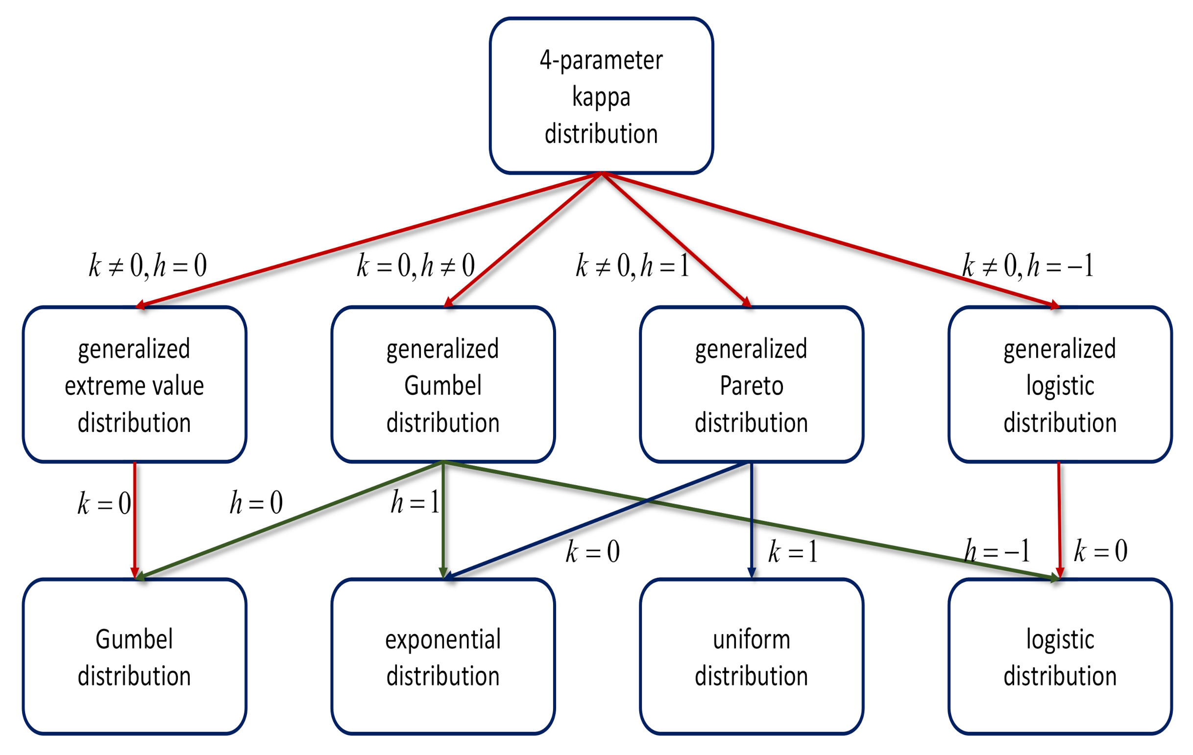
2. Four-Parameter Kappa Distribution
3. Maximum Likelihood and L-Moments Estimations
3.1. Maximum Likelihood Estimation
3.2. L-Moments Estimation
4. Bayesian Inference
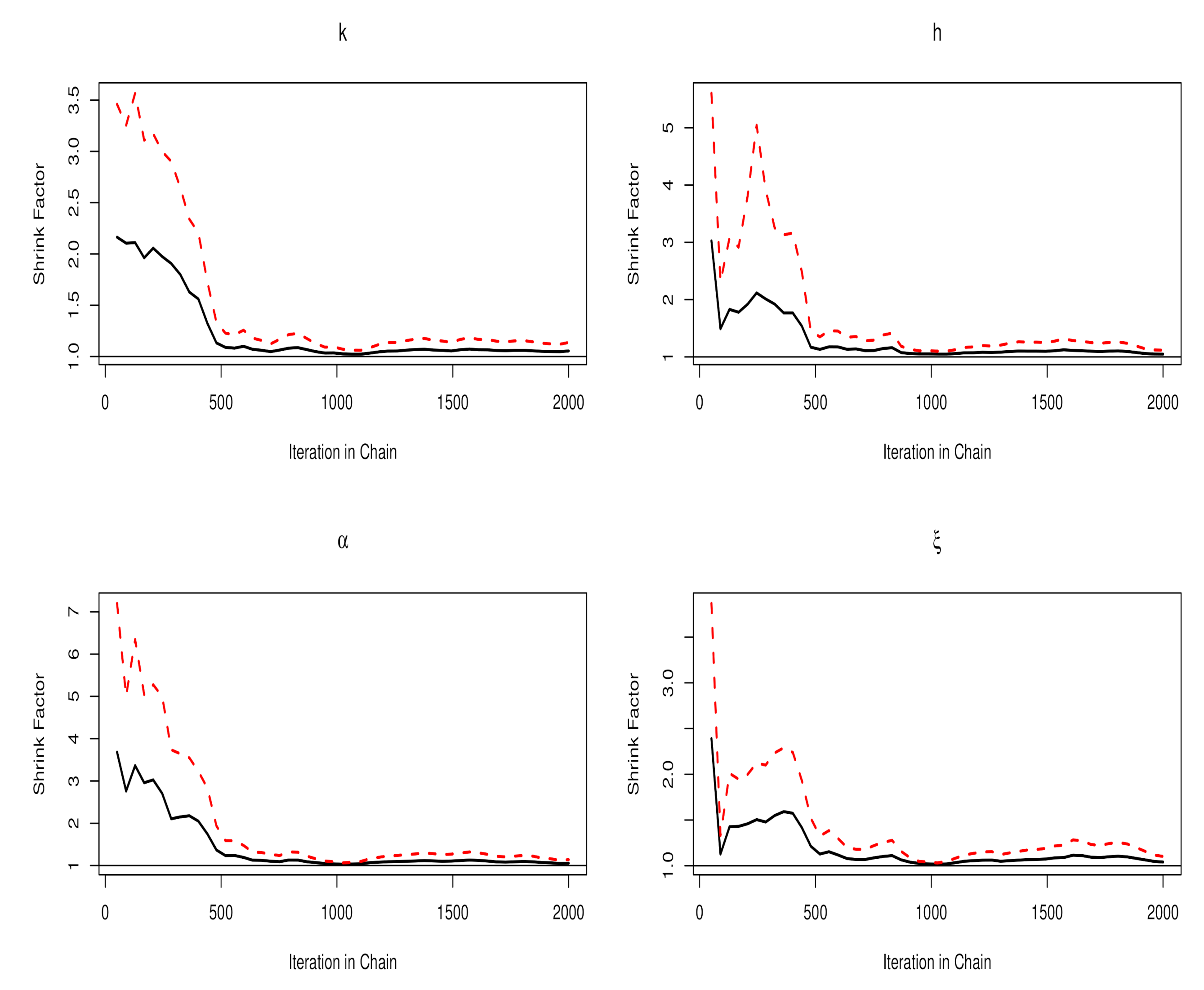
4.1. Computation by Markov Chain Monte Carlo
- Start with an initial value .
- For
- Generate a so-called “proposed value” , where the “proposed” standard deviation of k, is specified. Set:Accept:
- Generate a proposed value , where the proposed standard deviation of h, is specified. Set:Accept:
- Generate a proposed value , where the proposed standard deviation of , is specified. Set:Accept:
- Generate a proposed value , where the proposed standard deviation of , is specified. Set:Accept:
- Increase the counter from , and repeat Step 2.
- The final step is to transform our chain for using to regain our original scale parameter.
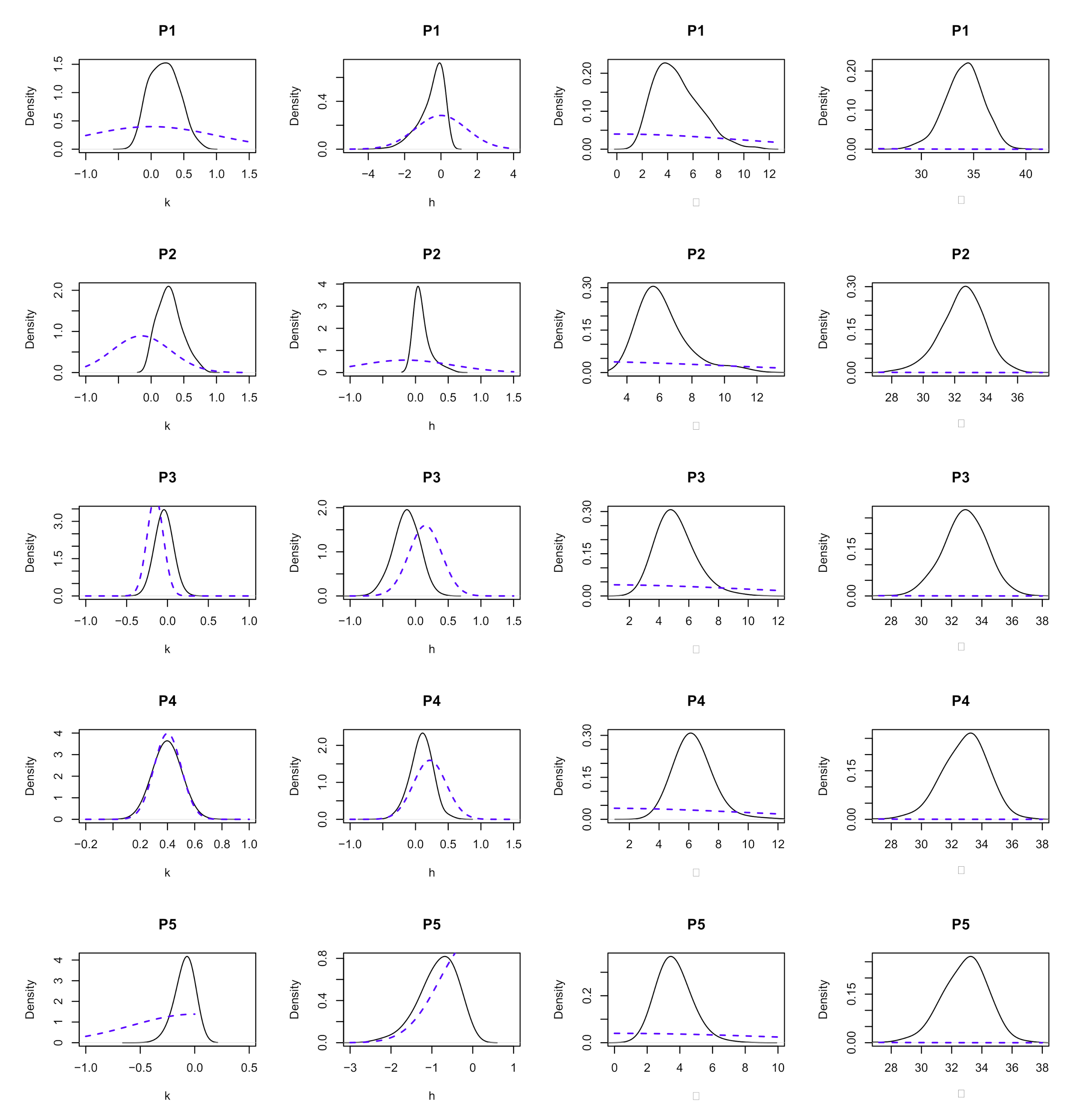
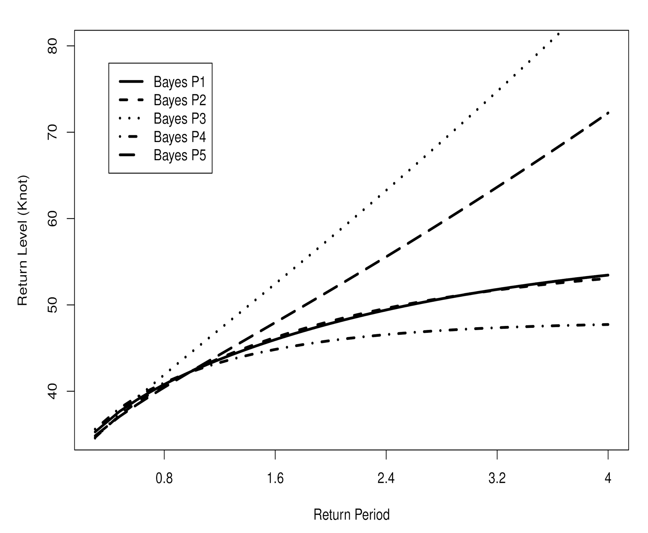
4.2. Prior Specification
- P1:
- Non-informative priors on all shape parameters: and . Given that the ranges of k and h are and , respectively, the variances of this prior make the distributions almost non-informative.
- P2:
- P3:
- Priors P3 are normal distributions with means of and 0.15, respectively, but with different variances reflecting different levels of uncertainty because there is no previous evidence on h. Note that the sign for h is positive: and .
- P4:
- Tight normal distributions around the shape parameter to assume the best scenario: and . In real applications, the mean values ( and , respectively) of k and h are estimated by LME from data.
- P5:
- When and , negative priors correspond to and , where and .
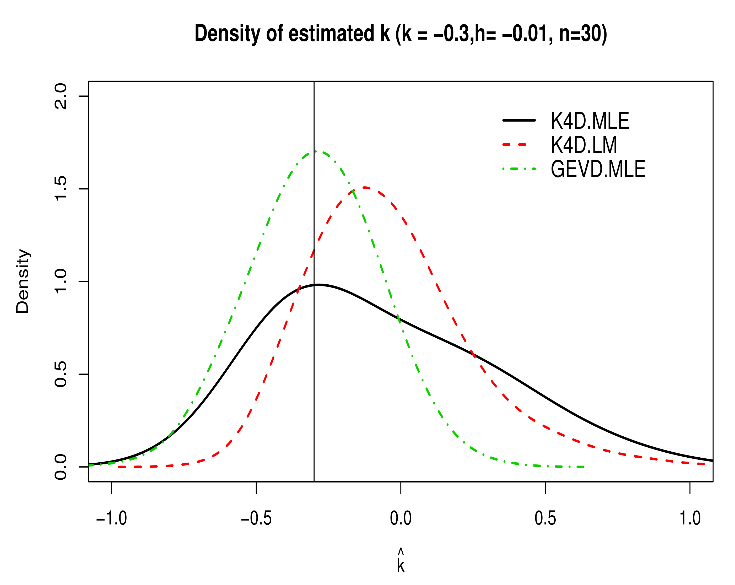
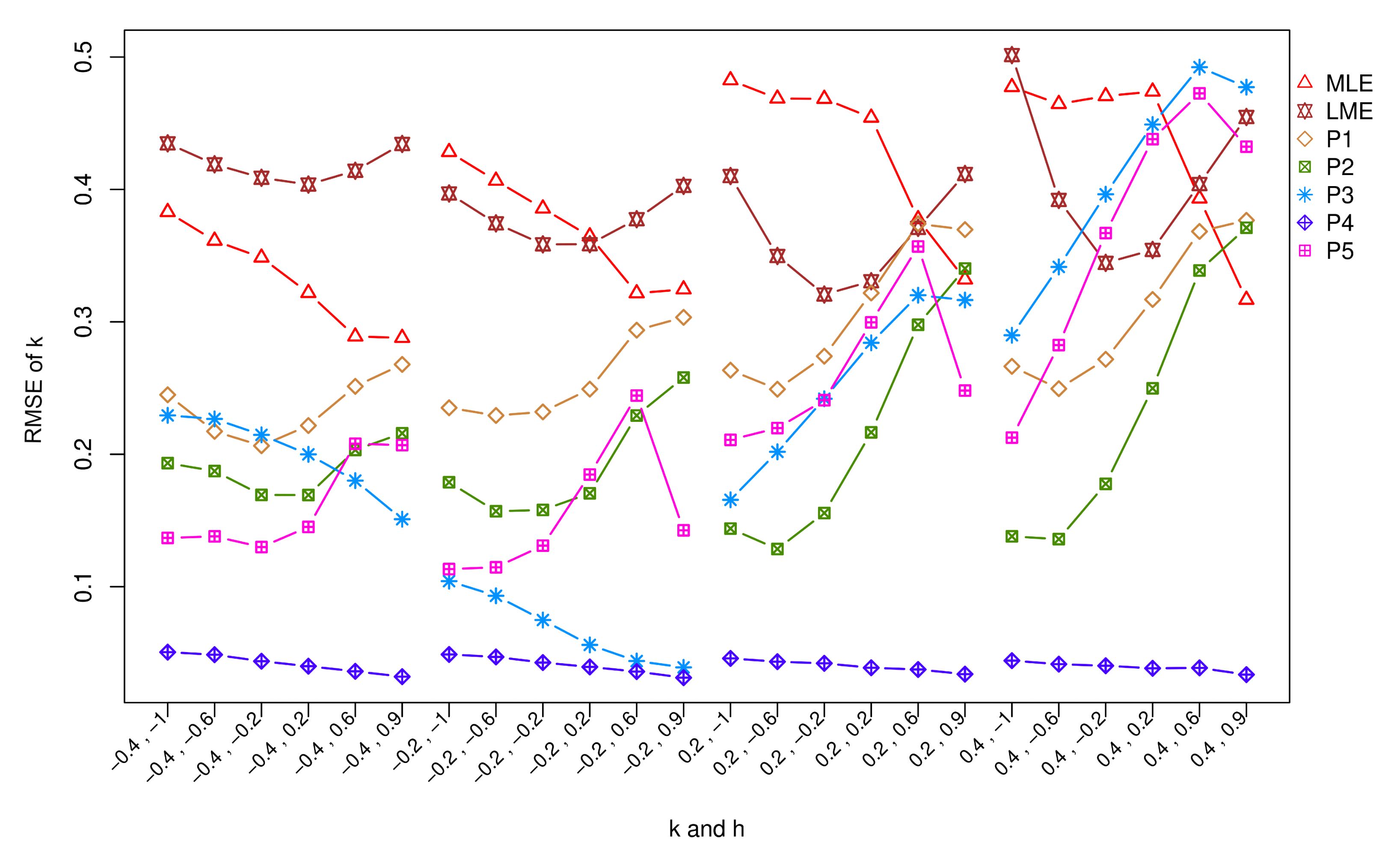
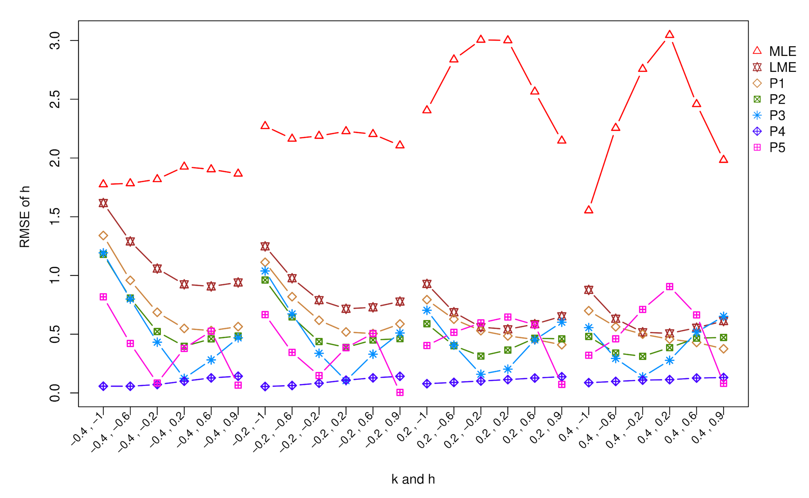
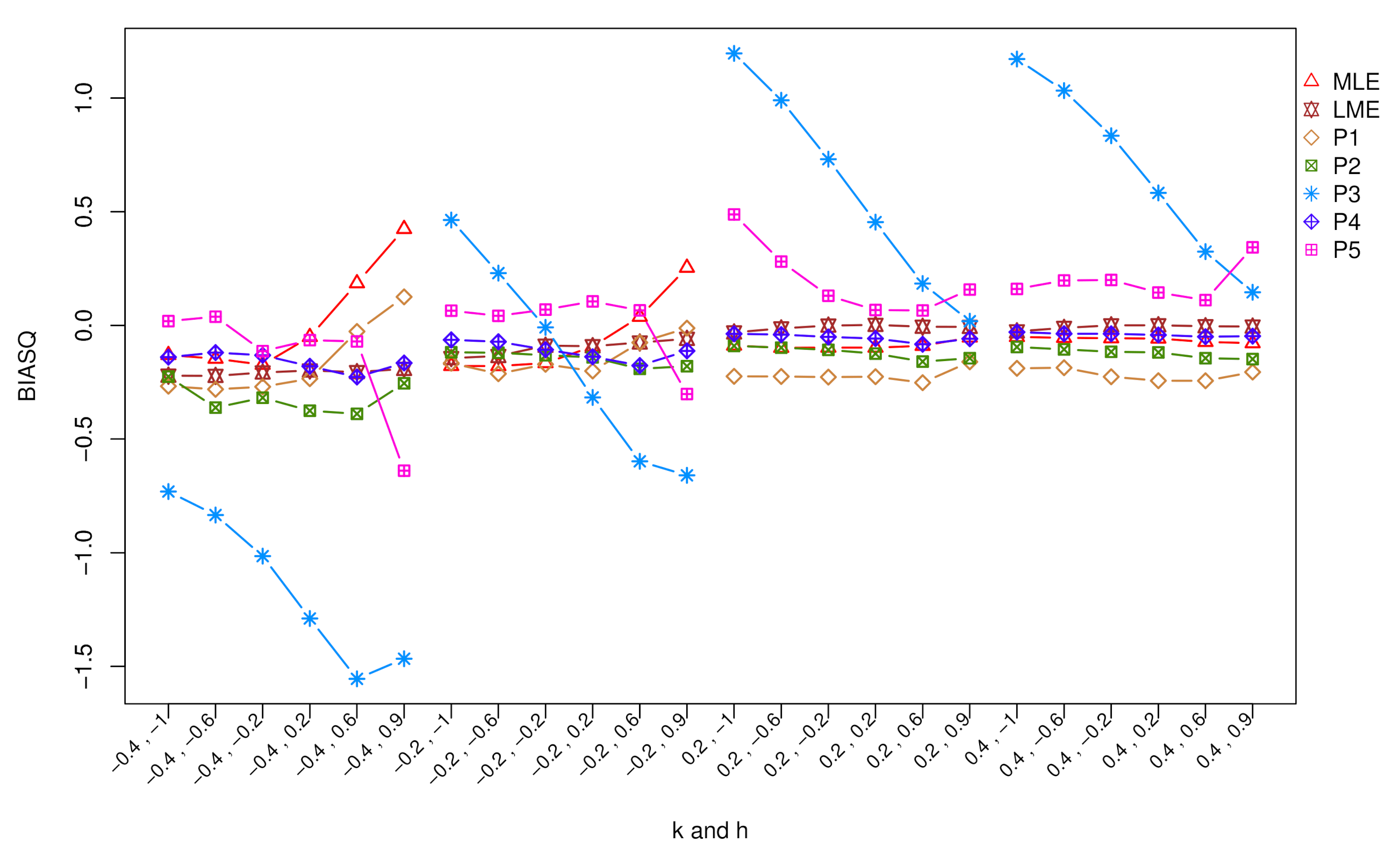
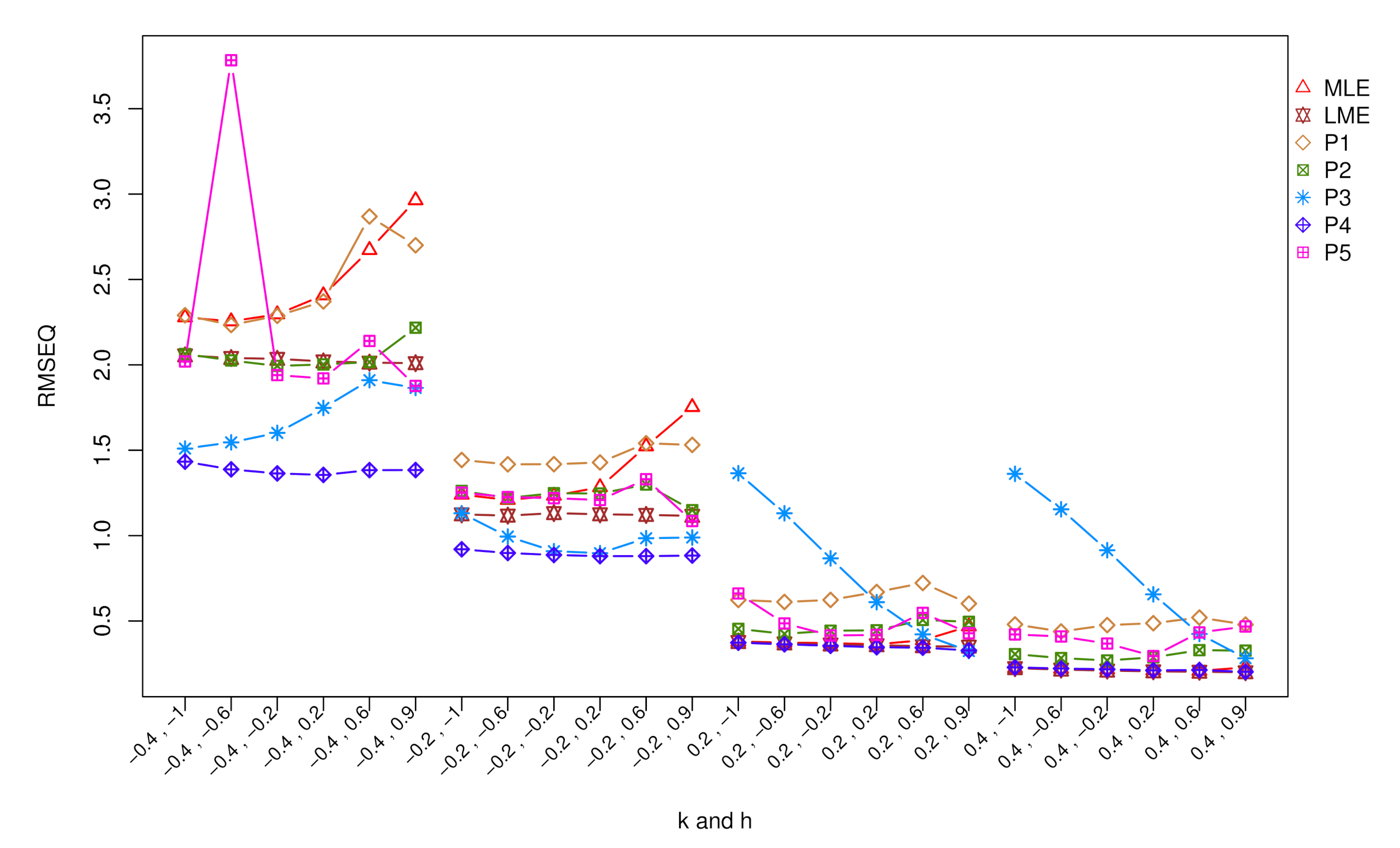
5. Simulation Study
6. Applications to Real-World Data
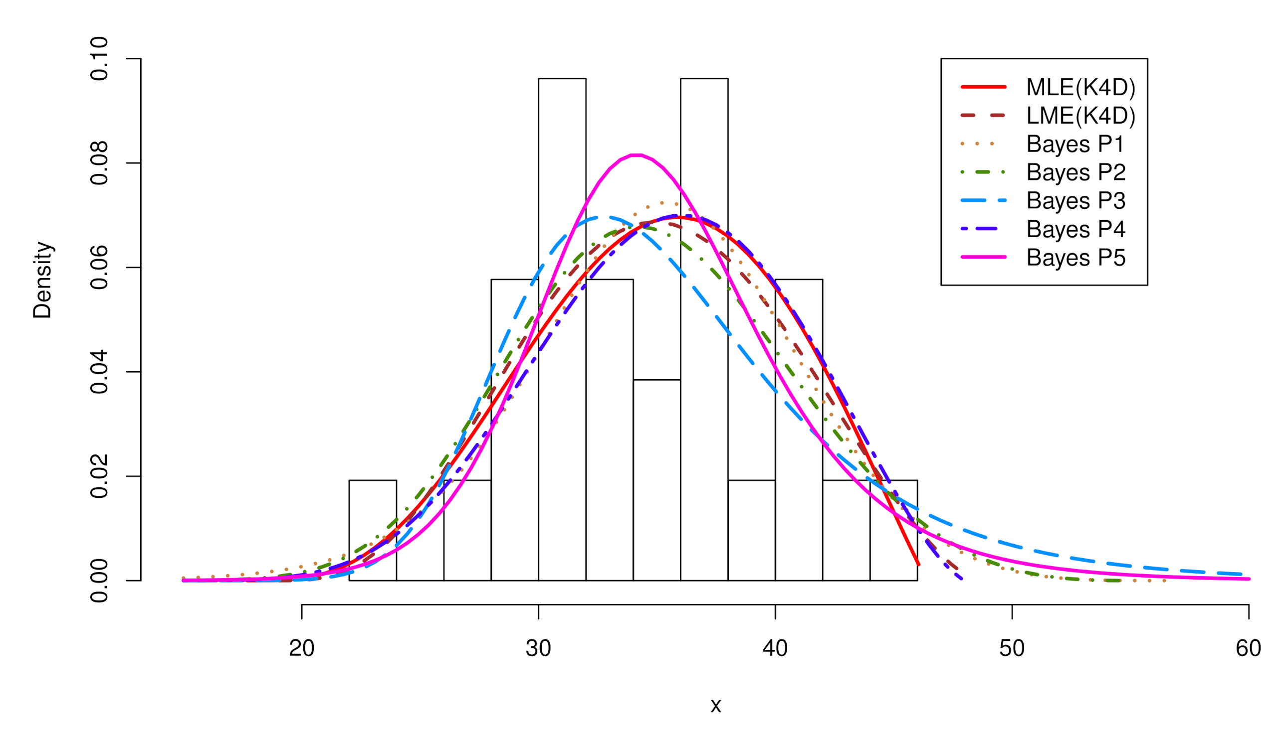
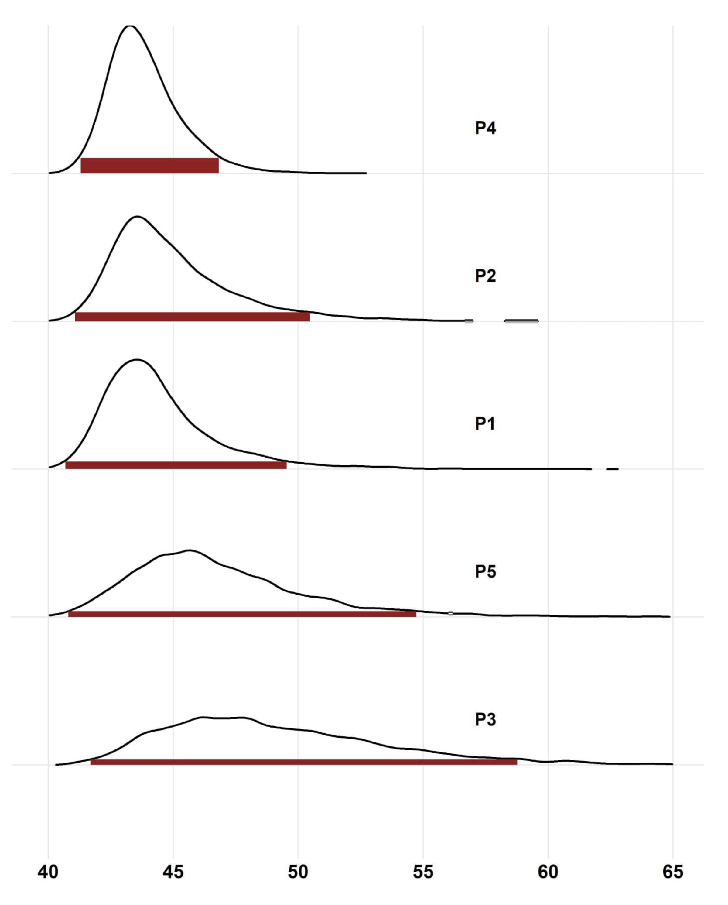
6.1. Maximum Wind Speeds in Udon Thani, Thailand
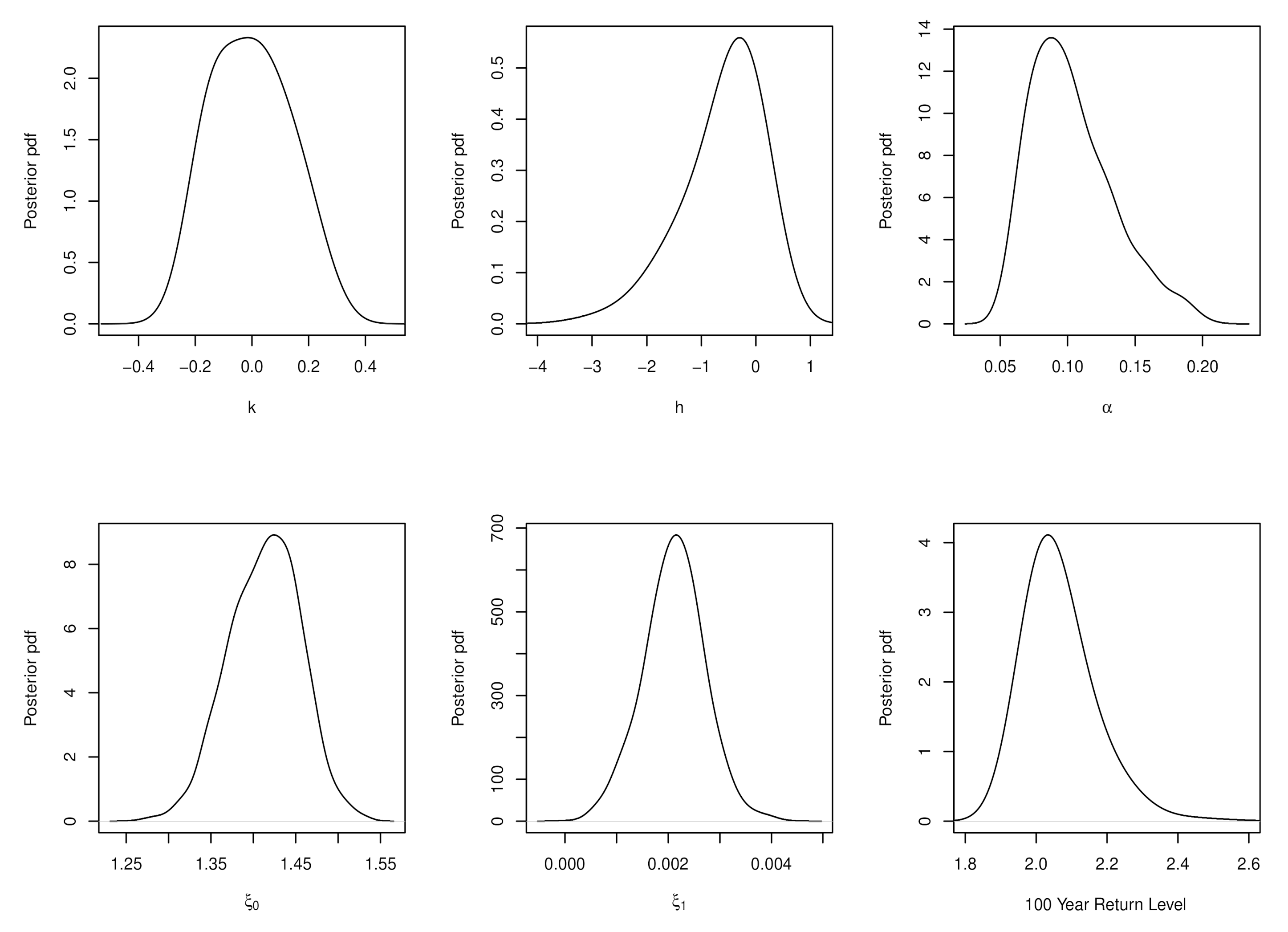
6.2. Maximum Sea-Levels at Fremantle, Australia: A Non-Stationary K4d
7. Conclusions and Discussion
Supplementary Materials
Author Contributions
Funding
Acknowledgments
Conflicts of Interest
References
- Hosking, J.R.M. The four-parameter kappa distribution. IBM J. Res. Dev. 1994, 38, 251–258. [Google Scholar] [CrossRef]
- Hosking, J.R.M.; Wallis, J.R. Regional Frequency Analysis: An Approach Based on L-Moments; Cambridge University Press: Cambridge, UK, 1997. [Google Scholar]
- Parida, B. Modelling of Indian summer monsoon rainfall using a four-parameter Kappa distribution. Int. J. Climatol. 1999, 19, 1389–1398. [Google Scholar] [CrossRef]
- Park, J.S.; Jung, H.S. Modelling Korean extreme rainfall using a Kappa distribution and maximum likelihood estimate. Theor. Appl. Climatol. 2002, 72, 55–64. [Google Scholar] [CrossRef]
- Singh, V.; Deng, Z. Entropy-based parameter estimation for kappa distribution. J. Hydrol. Eng. 2003, 8, 81–92. [Google Scholar] [CrossRef]
- Wallis, J.; Schaefer, M.; Barker, B.; Taylor, G. Regional precipitation-frequency analysis and spatial mapping for 24-hour and 2-hour durations for Washington State. Hydrol. Earth Syst. Sci. 2007, 11, 415–442. [Google Scholar] [CrossRef] [Green Version]
- Murshed, S.; Seo, Y.A.; Park, J.S. LH-moment estimation of a four parameter kappa distribution with hydrologic applications. Stoch. Environ. Res. Risk Assess. 2014, 28, 253–262. [Google Scholar] [CrossRef]
- Kjeldsen, T.R.; Ahn, H.; Prosdocimi, I. On the use of a four-parameter kappa distribution in regional frequency analysis. Hydrol. Sci. J. 2017, 62, 1354–1363. [Google Scholar] [CrossRef] [Green Version]
- Moses, O.; Parida, B.P. Statistical Modelling of Botswana s Monthly Maximum Wind Speed using a Four-Parameter Kappa Distribution. Am. J. Appl. Sci. 2016, 13, 773–778. [Google Scholar] [CrossRef] [Green Version]
- Blum, A.G.; Archfield, S.A.; Vogel, R.M. On the probability distribution of daily streamflow in the United States. Hydrol. Earth Syst. Sci. 2017, 21, 3093–3103. [Google Scholar] [CrossRef] [Green Version]
- Dupuis, D.; Winchester, C. More on the four-parameter kappa distribution. J. Stat. Comput. Simul. 2001, 71, 99–113. [Google Scholar] [CrossRef]
- Coles, S. An Introduction to Statistical Modeling of Extreme Values; Springer: London, UK, 2001. [Google Scholar]
- Coles, S.G.; Powell, E.A. Bayesian Methods in Extreme Value Modelling: A Review and New Developments. Int. Stat. Rev. 1996, 64, 119–136. [Google Scholar] [CrossRef]
- Coles, S.G.; Tawn, J.A. A Bayesian Analysis of Extreme Rainfall Data. J. R. Stat. Soc. Ser. C (Appl. Stat.) 1996, 45, 463–478. [Google Scholar] [CrossRef]
- Coles, S.G.; Tawn, J.A. Bayesian modelling of extreme surges on the UK east coast. Philos. Trans. R. Soc. Lond. A Math. Phys. Eng. Sci. 2005, 363, 1387–1406. [Google Scholar] [CrossRef] [PubMed]
- Vidal, I. A Bayesian analysis of the Gumbel distribution: An application to extreme rainfall data. Stoch. Environ. Res. Risk Assess. 2014, 28, 571–582. [Google Scholar] [CrossRef]
- Lima, C.H.; Kwon, H.H.; Kim, J.Y. A Bayesian beta distribution model for estimating rainfall IDF curves in a changing climate. J. Hydrol. 2016, 540, 744–756. [Google Scholar] [CrossRef]
- Lima, C.H.; Lall, U.; Troy, T.; Devineni, N. A hierarchical Bayesian GEV model for improving local and regional flood quantile estimates. J. Hydrol. 2016, 541, 816–823. [Google Scholar] [CrossRef]
- Fawcett, L.; Walshaw, D. Sea-surge and wind speed extremes: Optimal estimation strategies for planners and engineers. Stoch. Environ. Res. Risk Assess. 2016, 30, 463–480. [Google Scholar] [CrossRef]
- Fawcett, L.; Green, A.C. Bayesian posterior predictive return levels for environmental extremes. Stoch. Environ. Res. Risk Assess. 2018, 32, 2233–2252. [Google Scholar] [CrossRef] [Green Version]
- Russell, B.T. Investigating precipitation extremes in South Carolina with focus on the state’s October 2015 precipitation event. J. Appl. Stat. 2019, 46, 286–303. [Google Scholar] [CrossRef]
- Jeong, B.Y.; Murshed, M.S.; Seo, Y.A.; Park, J.S. A three-parameter kappa distribution with hydrologic application: A generalized gumbel distribution. Stoch. Environ. Res. Risk Assess. 2014, 28, 2063–2074. [Google Scholar] [CrossRef]
- Shin, Y.; Busababodhin, P.; Park, J.S. The r-largest four parameter kappa distribution. arXiv 2007, arXiv:2007.12031. [Google Scholar]
- R Core Team. R: A Language and Environment for Statistical Computing; R Foundation for Statistical Computing: Vienna, Austria, 2018. [Google Scholar]
- Park, J.S.; Park, B.J. Maximum likelihood estimation of the four-parameter Kappa distribution using the penalty method. Comput. Geosci. 2002, 28, 65–68. [Google Scholar] [CrossRef]
- Hosking, J.R.M. L-Moments: Analysis and Estimation of Distributions Using Linear Combinations of Order-Statistics. J. R. Stat. Soc. Ser. B (Methodol.) 1990, 52, 105–124. [Google Scholar] [CrossRef]
- Šimková, T. Confidence intervals based on L-moments for quantiles of the GP and GEV distributions with application to market-opening asset prices data. J. Appl. Stat. 2020, 1–28. [Google Scholar] [CrossRef]
- Bernardo, J.M.; Smith, A.F.M. Bayesian Theory; John Wiley and Sons: Hoboken, NJ, USA, 1994. [Google Scholar] [CrossRef]
- Metropolis, N.; Rosenbluth, A.W.; Rosenbluth, M.N.; Teller, A.H.; Teller, E. Equation of state calculations by fast computing machines. J. Chem. Phys. 1953, 21, 1087–1092. [Google Scholar] [CrossRef] [Green Version]
- Hastings, W.K. Monte Carlo Sampling Methods Using Markov Chains and Their Applications. Biometrika 1970, 57, 97–109. [Google Scholar] [CrossRef]
- Saraiva, E.F.; Suzuki, A.K.; Milan, L.A. Bayesian Computational Methods for Sampling from the Posterior Distribution of a Bivariate Survival Model, Based on AMH Copula in the Presence of Right-Censored Data. Entropy 2018, 20, 642. [Google Scholar] [CrossRef] [PubMed] [Green Version]
- Attia, A.; Moosavi, A.; Sandu, A. Cluster Sampling Filters for Non-Gaussian Data Assimilation. Atmosphere 2018, 9, 213. [Google Scholar] [CrossRef] [Green Version]
- Ariza-Hernandez, F.J.; Arciga-Alejandre, M.P.; Sanchez-Ortiz, J.; Fleitas-Imbert, A. Bayesian Derivative Order Estimation for a Fractional Logistic Model. Mathematics 2020, 8, 109. [Google Scholar] [CrossRef] [Green Version]
- Wasserman, L. All of Statistics: A Concise Course in Statistical Inference; Springer: Berlin, Germany, 2004. [Google Scholar]
- Ntzoufras, I. Bayesian Modeling Using WinBUGS; Wiley: Hoboken, NJ, USA, 2009. [Google Scholar]
- Martins, E.S.; Stedinger, J.R. Generalized maximum-likelihood generalized extreme-value quantile estimators for hydrologic data. Water Resour. Res. 2000, 36, 737–744. [Google Scholar] [CrossRef]
- Wilson, P.S.; Toumi, R. A fundamental probability distribution for heavy rainfall. Geophys. Res. Lett. 2005, 32, L14812. [Google Scholar] [CrossRef]
- Koutsoyiannis, D. Statistics of extremes and estimation of extreme rainfall: (ii) Empirical investigation of long rainfall records. Hydrol. Sci. J. 2004, 49, 591–610. [Google Scholar] [CrossRef]
- Carlin, B.P.; Louis, T.A. Bayes and Empirical Bayes Methods for Data Analysis, 2nd ed.; Texts in Statistical Science, Chapman and Hall: New York, NY, USA, 2000. [Google Scholar]
- Plummer, M.; Best, N.; Cowles, K.; Vines, K. CODA: Convergence Diagnosis and Output Analysis for MCMC. R News 2006, 6, 7–11. [Google Scholar]
- Gelman, A.; Carlin, J.; Stern, H.; Dunson, D.; Vehtari, A.; Rubin, D. Bayesian Data Analysis, 3rd ed.; CRC Press: Boca Raton, FL, USA, 2013. [Google Scholar]
- Liu, Y.; Lu, M.; Huo, X.; Hao, Y.; Gao, H.; Liu, Y.; Fan, Y.; Cui, Y.; Metivier, F. A Bayesian analysis of Generalized Pareto Distribution of runoff minima. Hydrol. Process. 2016, 30, 424–432. [Google Scholar] [CrossRef]


| Methods | Parameter Estimates | CIs of 20-Year Return Level | ||||||
|---|---|---|---|---|---|---|---|---|
| Lower | RL | Upper | Length | |||||
| Bayes P1 | 34.182 | 4.505 | 0.195 | −0.323 | 40.75 | 43.95 | 49.54 | 8.79 |
| (0.020) | (0.020) | (0.002) | (0.008) | (0.028) | ||||
| Bayes P2 | 32.647 | 5.637 | 0.248 | 0.009 | 41.07 | 43.55 | 50.47 | 9.40 |
| (0.016) | (0.017) | (0.002) | (0.001) | (0.028) | ||||
| Bayes P3 | 32.930 | 4.993 | −0.034 | −0.116 | 41.65 | 47.11 | 58.85 | 17.21 |
| (0.016) | (0.014) | (0.001) | (0.002) | (0.052) | ||||
| Bayes P4 | 33.356 | 6.085 | 0.414 | 0.106 | 41.30 | 43.20 | 46.86 | 5.57 |
| (0.017) | (0.014) | (0.001) | (0.002) | (0.016) | ||||
| Bayes P5 | 34.324 | 3.488 | −0.035 | −0.612 | 40.77 | 45.63 | 54.90 | 14.13 |
| (0.016) | (0.010) | (0.001) | (0.005) | (0.045) | ||||
| MLE(K4D) | 32.617 | 6.688 | 0.485 | 0.220 | 41.09 | 43.15 | 48.13 | 7.04 |
| (2.173) | (3.320) | (0.268) | (0.381) | (0.243) | ||||
| LME(K4D) | 32.401 | 6.507 | 0.401 | 0.219 | 41.69 | 43.70 | 46.42 | 4.73 |
| (1.096) | (5.126) | (0.017) | (0.021) | (0.043) | ||||
| MLE(GEV) | 33.431 | 5.281 | −0.363 | - | 41.07 | 43.02 | 47.87 | 6.80 |
| (1.148) | (0.841) | (0.141) | - | (1.202) | ||||
| LME(GEV) | 33.178 | 5.314 | 0.287 | - | 42.72 | 58.09 | 97.24 | 54.52 |
| (0.012) | (0.009) | (0.002) | - | (0.131) | ||||
| Methods | K-S-Test | A-D-test | Criterion | ||||
|---|---|---|---|---|---|---|---|
| stat | p | stat | p | AIC | BIC | DIC | |
| Bayes P1 | 0.122 | 0.836 | 0.357 | 0.889 | - | - | 164.94 |
| Bayes P2 | 0.135 | 0.726 | 0.393 | 0.855 | - | - | 164.38 |
| Bayes P3 | 0.120 | 0.847 | 0.509 | 0.736 | - | - | 168.02 |
| Bayes P4 | 0.136 | 0.718 | 0.394 | 0.853 | - | - | 162.98 |
| Bayes P5 | 0.148 | 0.618 | 0.383 | 0.864 | - | - | 166.61 |
| MLE(K4D) | 0.114 | 0.886 | 0.331 | 0.912 | 165.80 | 170.83 | - |
| LME(K4D) | 0.119 | 0.852 | 0.317 | 0.924 | 166.31 | 171.34 | - |
| MLE(GEV) | 0.125 | 0.811 | 0.350 | 0.895 | 166.06 | 171.09 | - |
| LME(GEV) | 0.177 | 0.389 | 1.388 | 0.206 | 189.33 | 194.36 | - |
| Iterations in Chain | Parameter | |||
|---|---|---|---|---|
| 100 | 1.62 (1.78) | 1.82 (2.04) | 2.07 (2.34) | 1.43 (1.55) |
| 200 | 1.41 (1.57) | 1.57 (1.82) | 1.75 (2.02) | 1.35 (1.48) |
| 500 | 1.11 (1.19) | 1.14 (1.24) | 1.17 (1.30) | 1.10 (1.17) |
| 1000 | 1.09 (1.18) | 1.09 (1.20) | 1.11 (1.22) | 1.07 (1.14) |
| 2000 | 1.05 (1.14) | 1.05 (1.12) | 1.06 (1.14) | 1.04 (1.10) |
| 5000 | 1.00 (1.01) | 1.00 (1.00) | 1.00 (1.00) | 1.02 (1.05) |
| Methods | Parameter Estimates | DIC | ||||
|---|---|---|---|---|---|---|
| GEV Bayes | −0.2296 | - | 0.1424 | 1.4816 | - | −81.1045 |
| GEV Bayes Non-stationary | −0.1138 | - | 0.1261 | 1.3639 | 0.0027 | −91.8363 |
| K4D Bayes P1 | 0.0101 | −0.2515 | 0.1115 | 1.5147 | - | −84.8245 |
| K4D Bayes P1 Non-stationary | 0.0001 | −0.1926 | 0.0891 | 1.4219 | 0.0021 | −104.3389 |
Publisher’s Note: MDPI stays neutral with regard to jurisdictional claims in published maps and institutional affiliations. |
© 2020 by the authors. Licensee MDPI, Basel, Switzerland. This article is an open access article distributed under the terms and conditions of the Creative Commons Attribution (CC BY) license (http://creativecommons.org/licenses/by/4.0/).
Share and Cite
Seenoi, P.; Busababodhin, P.; Park, J.-S. Bayesian Inference in Extremes Using the Four-Parameter Kappa Distribution. Mathematics 2020, 8, 2180. https://doi.org/10.3390/math8122180
Seenoi P, Busababodhin P, Park J-S. Bayesian Inference in Extremes Using the Four-Parameter Kappa Distribution. Mathematics. 2020; 8(12):2180. https://doi.org/10.3390/math8122180
Chicago/Turabian StyleSeenoi, Palakorn, Piyapatr Busababodhin, and Jeong-Soo Park. 2020. "Bayesian Inference in Extremes Using the Four-Parameter Kappa Distribution" Mathematics 8, no. 12: 2180. https://doi.org/10.3390/math8122180