Value at Risk Estimation Using the GARCH-EVT Approach with Optimal Tail Selection †


Abstract
:1. Introduction
2. Methods
2.1. Modeling Tail Using Extreme Value Theory
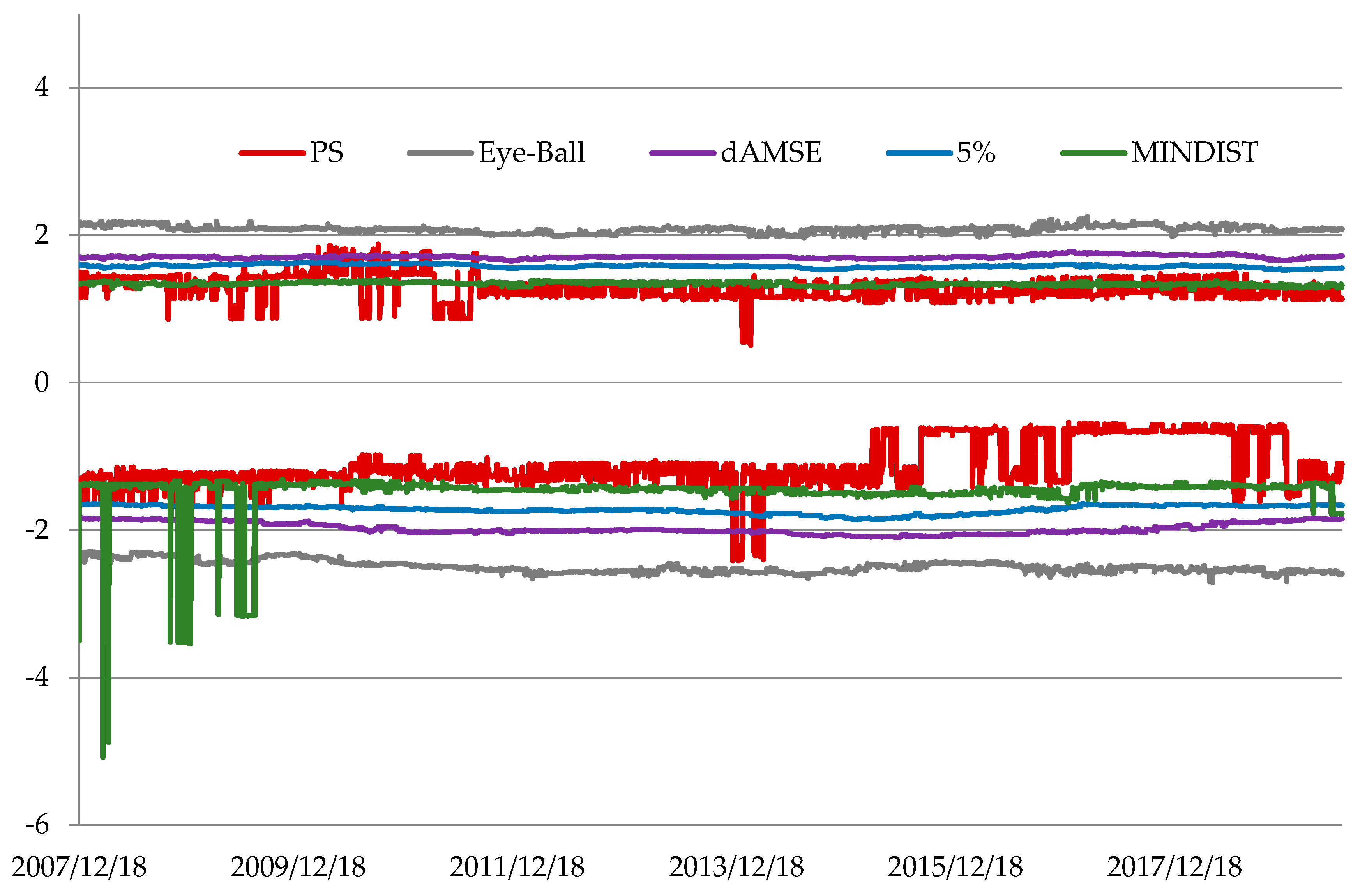
2.2. Optimal Tail Selection
2.2.1. Mean Absolute Deviation Distance Metric Method
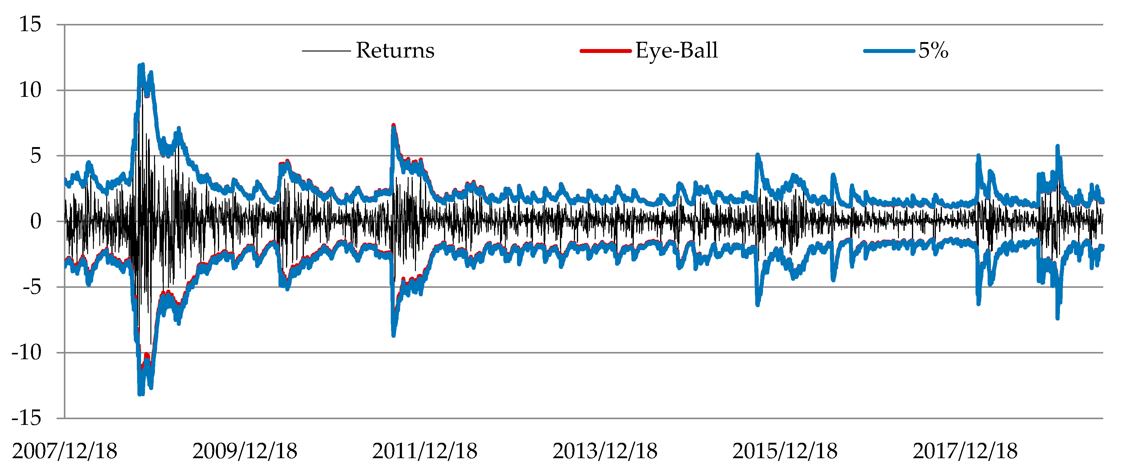
2.2.2. Eye-Ball Method
2.2.3. Path Stability Method
2.2.4. Minimization of Asymptotic Mean Squared Error Method
2.3. Conditional Extreme Value Theory Model
2.4. Backtesting
3. Results of Empirical Study
4. Conclusions
Author Contributions
Funding
Conflicts of Interest
References
- Pérignon, C.; Smith, D.R. The level and quantity of Value-at-Risk disclosure by commercial banks. J. Bank. Financ. 2010, 34, 362–377. [Google Scholar] [CrossRef]
- Loretan, M.; Phillips, P.C.B. Testing the covariance stationarity of heavy-tailed time series: An overview of the theory with applications to several financial datasets. J. Empir. Financ. 1994, 1, 211–248. [Google Scholar] [CrossRef]
- Danielsson, J.; de Vries, C.G. Tail index and quantile estimation with very high frequency data. J. Empir. Financ. 1997, 4, 241–257. [Google Scholar] [CrossRef] [Green Version]
- McNeil, A.J. Extreme Value Theory for Risk Managers. In Internal Modelling and CAD II; Risk Waters Group: London, UK, 1999; pp. 93–113. [Google Scholar]
- Neftic, S.N. Value at Risk Calculations, Extreme Events, and Tail Estimation. J. Deriv. 2000, 7, 23–38. [Google Scholar] [CrossRef]
- Longin, M. From value at risk to stress testing: The extreme value approach. J. Bank. Financ. 2000, 24, 1097–1130. [Google Scholar] [CrossRef]
- Diebold, F.X.; Schuermann, T.; Stroughair, J.D. Pitfalls and Opportunities in the Use of Extreme Value Theory in Risk Management. J. Risk Financ. 2000, 1, 30–36. [Google Scholar] [CrossRef] [Green Version]
- Jondeau, E.; Rockinger, M. Testing for differences in the tails of stock-market returns. J. Empir. Financ. 2003, 10, 559–581. [Google Scholar] [CrossRef] [Green Version]
- Fernandez, V. Risk management under extreme events. Int. Rev. Financ. Anal. 2005, 14, 113–148. [Google Scholar] [CrossRef]
- Gilli, M.; Kellezi, E. An Application of Extreme Value Theory for Measuring Financial Risk. Comput. Econ. 2006, 27, 207–228. [Google Scholar] [CrossRef] [Green Version]
- McNeil, A.J.; Frey, R. Estimation of tail-related risk measures for heteroskedastic financial time series: An extreme value approach. J. Empir. Financ. 2000, 7, 271–300. [Google Scholar] [CrossRef]
- Fernandez, V. Extreme value theory and value-at-risk. Rev. Anal. Econ. 2003, 18, 57–85. [Google Scholar]
- Jadhav, D.; Ramanathan, T.V. Parametric and non-papametric estimation of value-at-risk. J. Risk Model Valid. 2009, 3, 51–71. [Google Scholar] [CrossRef] [Green Version]
- Gençay, R.; Selçuk, F. Extreme value theory and Value at Risk: Relative performance in emerging markets. Int. J. Forecast. 2004, 20, 287–303. [Google Scholar] [CrossRef] [Green Version]
- Zhang, Z.; Zhang, H.K. The dynamics of precious metal markets VaR: A GARCHEVT approach. J. Commod. Mark. 2016, 4, 14–27. [Google Scholar] [CrossRef] [Green Version]
- Just, M. The use of Value-at-Risk models to estimate the investment risk on agricultural commodity market. In Proceedings of the International Conference Hradec Economic Days 2014: Economic Development and Management of Regions, Hradec Králové, Czech Republic, 3–4 February 2014; Jedlička, P., Ed.; University Hradec Králové: Hradec Králové, Czech Republic, 2014; Volume 4, pp. 264–273. [Google Scholar]
- Tabasi, H.; Yousefi, V.; Tamošaitienė, J.; Ghasemi, F. Estimating Conditional Value at Risk in the Teheran Stock Exchange Based on the Extreme Value Theory Using GARCH Models. Adm. Sci. 2019, 9, 40. [Google Scholar] [CrossRef] [Green Version]
- Coles, S.G. An Introduction to Statistical Modeling of Extreme Values; Springer Series in Statistics; Springer: London, UK, 2001. [Google Scholar]
- Karmakar, M.; Shukla, G.K. Managing extreme risk in some major stock markets: An extreme value approach. Int. Rev. Econ. Financ. 2015, 35, 1–25. [Google Scholar] [CrossRef]
- Bee, M.; Dupuis, D.J.; Trapin, L. Realizing the extremes: Estimation of tail-risk measures from a high-frequency perspective. J. Empir. Financ. 2016, 36, 86–99. [Google Scholar] [CrossRef]
- Totić, S.; Božović, M. Tail risk in emerging markets of Southeastern Europe. Appl. Econ. 2016, 48, 1785–1798. [Google Scholar] [CrossRef]
- Li, L. A Comparative Study of GARCH and EVT Model in Modeling Value-at-Risk. J. Appl. Bus. Econ. 2017, 19, 27–48. [Google Scholar]
- Huang, C.K.; North, D.; Zewotir, T. Exchangeability, extreme returns and Value-at-Risk forecasts. Phys. A 2017, 477, 204–216. [Google Scholar] [CrossRef]
- Cifter, A. Value-at-risk estimation with wavelet-based extreme value theory: Evidence from emerging markets. Phys. A 2011, 390, 2356–2367. [Google Scholar] [CrossRef]
- Soltane, H.B.; Karaa, A.; Bellalah, M. Conditional VaR using GARCH-EVT approach: Forecasting Volatility in Tunisian Financial Market. J. Comput. Model. 2012, 2, 95–115. [Google Scholar]
- Aboura, S. When the U.S. Stock Market Becomes Extreme? Risks 2014, 2, 211–225. [Google Scholar] [CrossRef] [Green Version]
- Omari, C.; Mwita, P.; Waititu, A. Using Conditional Extreme Value Theory to Estimate Value-at-Risk for Daily Currency Exchange Rates. J. Math. Financ. 2017, 7, 846–870. [Google Scholar] [CrossRef] [Green Version]
- Hill, B.M. A Simple General Approach to Inference About the Tail of a Distribution. Ann. Stat. 1975, 3, 1163–1174. [Google Scholar] [CrossRef]
- Pickands, J. Statistical inference using extreme order statistics. Ann. Stat. 1975, 3, 119–131. [Google Scholar]
- Dekkers, A.L.M.; Einmahl, J.H.J.; de Hann, L. A Moment Estimator for the Index of an Extreme-Value Distribution. Ann. Stat. 1989, 17, 1833–1855. [Google Scholar] [CrossRef]
- Hall, P. On some simple estimates of an exponent of regular variation. J. R. Stat. Soc. 1982, 44, 37–42. [Google Scholar] [CrossRef]
- Hall, P.; Welsh, A. Adaptive estimates of parameters of regular variation. Ann. Stat. 1985, 13, 331–341. [Google Scholar] [CrossRef]
- Danielsson, J.; de Haan, L.; Peng, L.; de Vries, C.G. Using a bootstrap method to choose the sample fraction in tail index estimation. J. Multivar. Anal. 2001, 76, 226–248. [Google Scholar] [CrossRef] [Green Version]
- Gomes, M.I.; Oliveira, O. The bootstrap methodology in statistics of extremes—Choice of the optimal sample fraction. Extremes 2001, 4, 331–358. [Google Scholar] [CrossRef]
- Hall, P. Using the Bootstrap to Estimate Mean Squared Error and Select Smoothing Parameter in Nonparametric Problems. J. Multivar. Anal. 1990, 32, 177–203. [Google Scholar] [CrossRef] [Green Version]
- Csörgő, S.; Viharos, L. Estimating the tail index. In Asymptotic Methods in Probability and Statistics; Szyszkowicz, B., Ed.; North-Holland: Amsterdam, The Netherlands, 1998; pp. 833–881. [Google Scholar]
- Danielsson, J.; Ergun, L.M.; de Haan, L.; de Vries, C.G. Tail Index Estimation: Quantile Driven Threshold Selection; SRC Working Paper, No. 58; Systemic Risk Centre, The London School of Economics and Political Science: London, UK, 2016. [Google Scholar]
- Caeiro, F.; Gomes, M.I. Threshold selection in extreme value analysis. In Extreme Value Modeling and Risk Analysis: Methods and Applications; Dipak, K.D., Jun, Y., Eds.; Taylor Francis: New York, NY, USA, 2016; pp. 69–86. [Google Scholar]
- Zhao, X.; Zhang, Z.; Cheng, W.; Zhang, P. A New Parameter Estimator for the Ganeralized Pareto Distribution under the Peaks over Threshold Fremwork. Mathematics 2019, 7, 406. [Google Scholar] [CrossRef] [Green Version]
- Echaust, K. Conditional Var Using GARCH-EVT Approach with Optimal Tail Selection. In Proceedings of the 10th Economics Finance Conference, Rome, Italy, 10–13 September 2018; Cermakova, K., Mozayeni, S., Hromada, E., Eds.; International Institute of Social and Economic Sciences: Prague, Czech Republic, 2018; pp. 105–118. [Google Scholar]
- Guégan, D.; Hassani, B. More accurate measurement for enhanced controls: VaR vs ES? J. Int. Financ. Mark. Inst. Money 2018, 54, 152–165. [Google Scholar] [CrossRef] [Green Version]
- Balkema, A.A.; de Haan, L. Residual Life Time at Great Age. Ann. Probab. 1974, 2, 792–804. [Google Scholar] [CrossRef]
- Ossberger, J. Tea: Threshold Estimation Approaches, R package, Version 1.0; 2017. Available online: https://cran.r-project.org/web/packages/tea/index.html (accessed on 27 October 2019).
- Bollerslev, T. Generalized autoregressive conditional heteroskedasticity. J. Econom. 1986, 31, 307–327. [Google Scholar] [CrossRef] [Green Version]
- Kupiec, P.H. Techniques for Verifying the Accuracy of Risk Measurement Models. J. Deriv. 1995, 3, 73–84. [Google Scholar] [CrossRef]
- Christoffersen, P.F. Evaluating Interval Forecasts. Int. Econ. Rev. 1998, 39, 841–862. [Google Scholar] [CrossRef]
- Christoffersen, P.F.; Pelletier, D. Backtesting Value-at-Risk: A Duration-Based Approach. J. Financ. Econom. 2004, 2, 84–108. [Google Scholar] [CrossRef]
- Engle, R.F.; Manganelli, S. CAViaR: Conditional Autoregressive Value at Risk by Regression Quantiles. J. Bus. Econ. Stat. 2004, 22, 367–381. [Google Scholar] [CrossRef]
- Kuester, K.; Mittnik, S.; Paolella, M.S. Value-at-Risk Prediction: A Comparison of Alternative Strategies. J. Financ. Econom. 2006, 4, 53–89. [Google Scholar] [CrossRef] [Green Version]
- Gonzalez-Rivera, G.; Lee, T.-H.; Mishra, S. Forecasting Volatility: A Reality Check Based on Option Pricing, Utility Function, Value-at-Risk, and Predictive Likelihood. Int. J. Forecast. 2004, 20, 629–645. [Google Scholar] [CrossRef]
- Financial Stock News Website. Available online: www.stooq.pl (accessed on 26 October 2019).
- Wuertz, D.; Setz, T.; Chalabi, Y.; Boudt, C.; Chausse, P.; Miklovac, M. fGarch: Rmetrics—Autoregressive Conditional Heteroskedastic Modelling, R package, Version 3042.83; 2017. Available online: https://cran.r-project.org/web/packages/fGarch/index.html (accessed on 31 January 2019).
- Pfaff, B.; McNeil, A.; Stephenson, A. evir: Extreme Values in R, R package, Version 1.7-3; 2012. Available online: https://cran.r-project.org/web/packages/evir/index.html (accessed on 31 January 2019).
- Guégan, D.; Hassani, B.; Naud, C. An efficient threshold choice for the computation of operational risk capital. J. Oper. Risk 2011, 6, 3–19. [Google Scholar] [CrossRef]
- McAleer, M.; Da Veiga, B. Forecasting Value-at-Risk with a Parsimonious Portfolio Spillover GARCH (PS-GARCH) Model. J. Forecast. 2008, 27, 1–19. [Google Scholar] [CrossRef] [Green Version]
- Ghalanos, A. Rugach: Univariate GARCH Models, R package, Version 1.4-0; 2018. Available online: https://cran.r-project.org/web/packages/rugarch/index.html (accessed on 31 January 2019).
- Catania, L.; Boudt, K.; Ardia, D. GAS: Generalized Autoregressive Score Models, R package, Version 0.3.0; 2019. Available online: https://cran.r-project.org/web/packages/GAS/index.html (accessed on 31 October 2019).


| Lower Tail | Upper Tail | |||||||
|---|---|---|---|---|---|---|---|---|
| SPX | Max | Mean | Min | StDev | Min | Mean | Max | StDev |
| PS | −2.416 | −1.115 | −0.541 | 0.308 | 0.504 | 1.284 | 1.880 | 0.164 |
| Eye-Ball | −2.713 | −2.499 | −2.290 | 0.080 | 1.963 | 2.081 | 2.253 | 0.045 |
| dAMSE | −2.103 | −1.979 | −1.831 | 0.076 | 1.648 | 1.706 | 1.777 | 0.022 |
| 5% | −1.861 | −1.720 | −1.638 | 0.055 | 1.525 | 1.580 | 1.631 | 0.023 |
| MINDIST | −5.083 | −1.483 | −1.317 | 0.304 | 1.267 | 1.339 | 1.396 | 0.023 |
| UKX | Max | Mean | Min | StDev | Min | Mean | Max | StDev |
| PS | −1.738 | −1.022 | −0.423 | 0.303 | 0.444 | 1.194 | 2.010 | 0.435 |
| Eye-Ball | −2.621 | −2.396 | −2.276 | 0.061 | 1.865 | 2.064 | 2.217 | 0.068 |
| dAMSE | −2.011 | −1.942 | −1.875 | 0.035 | 1.633 | 1.702 | 1.757 | 0.029 |
| 5% | −1.784 | −1.741 | −1.670 | 0.021 | 1.515 | 1.587 | 1.656 | 0.028 |
| MINDIST | −1.620 | −1.478 | −1.336 | 0.052 | 1.263 | 1.400 | 4.066 | 0.327 |
| CAC | Max | Mean | Min | StDev | Min | Mean | Max | StDev |
| PS | −2.239 | −1.152 | −0.579 | 0.333 | 0.697 | 1.241 | 1.643 | 0.116 |
| Eye-Ball | −2.594 | −2.430 | −2.288 | 0.046 | 1.859 | 2.112 | 2.365 | 0.075 |
| dAMSE | −1.967 | −1.888 | −1.811 | 0.033 | 1.629 | 1.678 | 1.747 | 0.021 |
| 5% | −1.763 | −1.718 | −1.661 | 0.021 | 1.523 | 1.562 | 1.620 | 0.018 |
| MINDIST | −5.506 | −1.955 | −1.298 | 0.991 | 1.223 | 1.324 | 3.755 | 0.163 |
| DAX | Max | Mean | Min | StDev | Min | Mean | Max | StDev |
| PS | −2.173 | −1.260 | −0.506 | 0.333 | 0.473 | 1.123 | 2.059 | 0.340 |
| Eye-Ball | −2.568 | −2.428 | −2.238 | 0.074 | 1.975 | 2.095 | 2.322 | 0.075 |
| dAMSE | −1.986 | −1.926 | −1.853 | 0.034 | 1.696 | 1.742 | 1.801 | 0.021 |
| 5% | −1.784 | −1.724 | −1.660 | 0.026 | 1.565 | 1.621 | 1.670 | 0.019 |
| MINDIST | −4.510 | −1.627 | −1.378 | 0.521 | 1.275 | 1.365 | 4.614 | 0.071 |
| OMXS | Max | Mean | Min | StDev | Min | Mean | Max | StDev |
| PS | −2.249 | −1.170 | −0.611 | 0.354 | 0.837 | 1.047 | 1.429 | 0.117 |
| Eye-Ball | −2.584 | −2.369 | −2.178 | 0.082 | 1.996 | 2.128 | 2.304 | 0.057 |
| dAMSE | −1.967 | −1.904 | −1.804 | 0.034 | 1.664 | 1.718 | 1.802 | 0.030 |
| 5% | −1.764 | −1.684 | −1.595 | 0.046 | 1.533 | 1.590 | 1.646 | 0.026 |
| MINDIST | −5.900 | −1.491 | −1.312 | 0.440 | 1.278 | 1.348 | 1.482 | 0.042 |
| KOSPI | Max | Mean | Min | StDev | Min | Mean | Max | StDev |
| PS | −2.285 | −1.106 | −0.635 | 0.371 | 0.560 | 1.251 | 1.993 | 0.205 |
| Eye-Ball | −2.680 | −2.481 | −2.290 | 0.061 | 1.889 | 2.063 | 2.197 | 0.056 |
| dAMSE | −2.105 | −2.032 | −1.916 | 0.044 | 1.642 | 1.684 | 1.721 | 0.015 |
| 5% | −1.857 | −1.771 | −1.684 | 0.044 | 1.530 | 1.578 | 1.627 | 0.020 |
| MINDIST | −6.799 | −1.584 | −1.386 | 0.421 | 1.227 | 1.317 | 1.388 | 0.028 |
| NKX | Max | Mean | Min | StDev | Min | Mean | Max | StDev |
| PS | −2.103 | −1.365 | −0.623 | 0.257 | 0.648 | 1.368 | 1.905 | 0.223 |
| Eye-Ball | −2.706 | −2.421 | −2.249 | 0.110 | 1.844 | 1.980 | 2.202 | 0.067 |
| dAMSE | −1.955 | −1.904 | −1.821 | 0.030 | 1.624 | 1.682 | 1.761 | 0.027 |
| 5% | −1.780 | −1.728 | −1.629 | 0.036 | 1.524 | 1.561 | 1.606 | 0.016 |
| MINDIST | −7.455 | −2.331 | −1.341 | 0.788 | 1.292 | 1.407 | 4.101 | 0.394 |
| HSI | Max | Mean | Min | StDev | Min | Mean | Max | StDev |
| PS | −2.006 | −1.340 | −0.992 | 0.206 | 0.821 | 1.352 | 2.053 | 0.360 |
| Eye-Ball | −2.687 | −2.402 | −2.119 | 0.127 | 1.978 | 2.111 | 2.244 | 0.053 |
| dAMSE | −1.902 | −1.845 | −1.805 | 0.017 | 1.687 | 1.749 | 1.865 | 0.031 |
| 5% | −1.720 | −1.680 | −1.636 | 0.015 | 1.562 | 1.620 | 1.718 | 0.040 |
| MINDIST | −4.866 | −1.454 | −1.346 | 0.386 | 1.307 | 1.719 | 4.628 | 0.938 |
| BVP | Max | Mean | Min | StDev | Min | Mean | Max | StDev |
| PS | −2.358 | −1.134 | −0.611 | 0.253 | 1.024 | 1.273 | 1.893 | 0.148 |
| Eye-Ball | −2.473 | −2.312 | −2.127 | 0.074 | 1.967 | 2.122 | 2.316 | 0.048 |
| dAMSE | −1.882 | −1.815 | −1.748 | 0.030 | 1.656 | 1.710 | 1.764 | 0.022 |
| 5% | −1.733 | −1.678 | −1.585 | 0.038 | 1.560 | 1.597 | 1.643 | 0.018 |
| MINDIST | −5.372 | −1.710 | −1.306 | 0.529 | 1.254 | 1.353 | 2.641 | 0.145 |
| AOR | Max | Mean | Min | StDev | Min | Mean | Max | StDev |
| PS | −2.213 | −1.052 | −0.791 | 0.101 | 0.796 | 1.095 | 1.964 | 0.173 |
| Eye-Ball | −2.750 | −2.461 | −2.268 | 0.087 | 1.907 | 2.011 | 2.087 | 0.028 |
| dAMSE | −2.015 | −1.952 | −1.842 | 0.040 | 1.601 | 1.644 | 1.694 | 0.022 |
| 5% | −1.784 | −1.708 | −1.612 | 0.036 | 1.496 | 1.545 | 1.603 | 0.025 |
| MINDIST | −4.639 | −1.786 | −1.349 | 0.913 | 1.262 | 1.318 | 2.618 | 0.035 |
| SPX Lower Tail | UKX Upper Tail | CAC Lower Tail | CAC Upper Tail | DAX Lower Tail | DAX Upper Tail | OMXS Lower Tail | KOSPI Lower Tail | |
| Number of moving windows without estimating Generalized Pareto Distribution (GPD) parameters | 3 | 22 | 334 | 9 | 47 | 1 | 30 | 8 |
| Number of moving windows | 2902 | 2924 | 2982 | 2982 | 2948 | 2948 | 2891 | 2811 |
| Percentage of moving windows without estimating GPD parameters | 0.10 | 0.75 | 11.20 | 0.30 | 1.59 | 0.03 | 1.04 | 0.28 |
| NKX Lower Tail | NKX Upper Tail | HSI Lower Tail | HSI Upper Tail | BVP Lower Tail | BVP Upper Tail | AOR Lower Tail | ||
| Number of moving windows without estimating GPD parameters | 552 | 59 | 41 | 270 | 19 | 27 | 198 | |
| Number of moving windows | 2781 | 2781 | 2803 | 2803 | 2821 | 2821 | 2927 | |
| Percentage of moving windows without estimating GPD parameters | 19.85 | 2.12 | 1.46 | 9.63 | 0.67 | 0.96 | 6.76 |
| Lower Tail, VaR 0.01 | Upper Tail, VaR 0.99 | |||||||
|---|---|---|---|---|---|---|---|---|
| SPX | Max | Mean | Min | StDev | Min | Mean | Max | StDev |
| PS | −13.170 | −2.910 | −1.312 | 1.695 | 1.072 | 2.449 | 11.897 | 1.517 |
| Eye-Ball | −12.647 | −2.819 | −1.306 | 1.620 | 1.072 | 2.482 | 11.917 | 1.530 |
| dAMSE | −13.001 | −2.878 | −1.313 | 1.669 | 1.078 | 2.472 | 11.959 | 1.529 |
| 5% | −13.192 | −2.915 | −1.329 | 1.691 | 1.084 | 2.471 | 11.970 | 1.527 |
| MINDIST | x | x | x | x | 1.076 | 2.458 | 11.934 | 1.520 |
| UKX | Max | Mean | Min | StDev | Min | Mean | Max | StDev |
| PS | −14.349 | −2.854 | −1.228 | 1.530 | 1.018 | 2.412 | 11.371 | 1.213 |
| Eye-Ball | −14.191 | −2.847 | −1.225 | 1.520 | 1.015 | 2.347 | 11.251 | 1.193 |
| dAMSE | −14.135 | −2.841 | −1.219 | 1.514 | 1.026 | 2.376 | 11.305 | 1.203 |
| 5% | −14.121 | −2.842 | −1.225 | 1.509 | 1.042 | 2.389 | 11.415 | 1.212 |
| MINDIST | −14.207 | −2.855 | −1.229 | 1.528 | x | x | x | x |
| CAC | Max | Mean | Min | StDev | Min | Mean | Max | StDev |
| PS | −14.763 | −3.523 | −1.481 | 1.667 | 1.334 | 3.061 | 12.235 | 1.371 |
| Eye-Ball | −13.665 | −3.369 | −1.470 | 1.533 | 1.368 | 3.049 | 12.080 | 1.349 |
| dAMSE | −13.624 | −3.395 | −1.486 | 1.530 | 1.325 | 3.055 | 12.134 | 1.365 |
| 5% | −13.919 | −3.424 | −1.479 | 1.567 | 1.326 | 3.048 | 12.161 | 1.362 |
| MINDIST | x | x | x | x | x | x | x | x |
| DAX | Max | Mean | Min | StDev | Min | Mean | Max | StDev |
| PS | −13.571 | −3.417 | −1.504 | 1.529 | 1.425 | 3.015 | 11.543 | 1.284 |
| Eye-Ball | −12.837 | −3.278 | −1.474 | 1.438 | 1.348 | 2.966 | 11.032 | 1.252 |
| dAMSE | −12.829 | −3.316 | −1.505 | 1.452 | 1.361 | 2.961 | 11.141 | 1.259 |
| 5% | −13.095 | −3.365 | −1.510 | 1.480 | 1.383 | 2.979 | 11.296 | 1.274 |
| MINDIST | x | x | x | x | x | x | x | x |
| OMXS | Max | Mean | Min | StDev | Min | Mean | Max | StDev |
| PS | −11.838 | −3.361 | −1.469 | 1.637 | 1.326 | 2.993 | 10.483 | 1.423 |
| Eye-Ball | −12.185 | −3.358 | −1.386 | 1.684 | 1.327 | 2.988 | 10.367 | 1.411 |
| dAMSE | −12.115 | −3.349 | −1.419 | 1.666 | 1.324 | 3.004 | 10.398 | 1.417 |
| 5% | −12.048 | −3.377 | −1.425 | 1.675 | 1.324 | 3.000 | 10.374 | 1.410 |
| MINDIST | x | x | x | x | 1.325 | 3.017 | 10.570 | 1.434 |
| KOSPI | Max | Mean | Min | StDev | Min | Mean | Max | StDev |
| PS | −15.382 | −2.958 | −1.484 | 1.569 | 1.216 | 2.465 | 13.476 | 1.381 |
| Eye-Ball | −14.804 | −2.860 | −1.424 | 1.514 | 1.224 | 2.464 | 13.148 | 1.353 |
| dAMSE | −15.063 | −2.865 | −1.448 | 1.535 | 1.226 | 2.470 | 13.282 | 1.368 |
| 5% | −15.412 | −2.941 | −1.486 | 1.570 | 1.218 | 2.458 | 13.215 | 1.361 |
| MINDIST | x | x | x | x | 1.217 | 2.472 | 13.371 | 1.382 |
| NKX | Max | Mean | Min | StDev | Min | Mean | Max | StDev |
| PS | −17.531 | −3.810 | −1.945 | 1.815 | 1.549 | 3.119 | 15.191 | 1.547 |
| Eye-Ball | −17.391 | −3.703 | −1.825 | 1.772 | 1.557 | 3.097 | 14.479 | 1.478 |
| dAMSE | −17.404 | −3.719 | −1.847 | 1.777 | 1.556 | 3.108 | 14.675 | 1.495 |
| 5% | −17.531 | −3.763 | −1.873 | 1.789 | 1.551 | 3.125 | 14.888 | 1.522 |
| MINDIST | x | x | x | x | x | x | x | x |
| HSI | Max | Mean | Min | StDev | Min | Mean | Max | StDev |
| PS | −18.454 | −3.524 | −1.684 | 1.858 | 1.570 | 3.182 | 16.768 | 1.688 |
| Eye-Ball | −17.963 | −3.559 | −1.729 | 1.811 | 1.546 | 3.165 | 16.881 | 1.713 |
| dAMSE | −17.924 | −3.513 | −1.700 | 1.791 | 1.547 | 3.156 | 16.836 | 1.707 |
| 5% | −18.104 | −3.516 | −1.681 | 1.815 | 1.565 | 3.173 | 16.776 | 1.702 |
| MINDIST | x | x | x | x | x | x | x | x |
| BVP | Max | Mean | Min | StDev | Min | Mean | Max | StDev |
| PS | −16.900 | −4.128 | −2.667 | 1.571 | 2.430 | 3.710 | 13.812 | 1.251 |
| Eye-Ball | −15.850 | −3.981 | −2.537 | 1.452 | 2.423 | 3.726 | 13.790 | 1.230 |
| dAMSE | −16.218 | −3.985 | −2.533 | 1.509 | 2.437 | 3.725 | 13.820 | 1.246 |
| 5% | −16.279 | −3.993 | −2.575 | 1.499 | 2.443 | 3.713 | 13.849 | 1.247 |
| MINDIST | x | x | x | x | x | x | x | x |
| AOR | Max | Mean | Min | StDev | Min | Mean | Max | StDev |
| PS | −11.313 | −2.598 | −1.147 | 1.279 | 0.975 | 2.126 | 9.146 | 1.016 |
| Eye-Ball | −10.784 | −2.529 | −1.143 | 1.213 | 0.972 | 2.121 | 8.809 | 0.980 |
| dAMSE | −10.986 | −2.548 | −1.154 | 1.230 | 0.966 | 2.135 | 8.961 | 1.000 |
| 5% | −11.188 | −2.602 | −1.156 | 1.263 | 0.961 | 2.126 | 9.005 | 1.009 |
| MINDIST | x | x | x | x | 0.977 | 2.124 | 9.040 | 1.012 |
| Lower Tail, VaR 0.005 | Upper Tail, VaR 0.995 | |||||||
|---|---|---|---|---|---|---|---|---|
| SPX | Max | Mean | Min | StDev | Min | Mean | Max | StDev |
| PS | −15.376 | −3.369 | −1.525 | 1.981 | 1.206 | 2.716 | 13.192 | 1.681 |
| Eye-Ball | −14.556 | −3.209 | −1.532 | 1.857 | 1.197 | 2.742 | 13.195 | 1.689 |
| dAMSE | −15.094 | −3.308 | −1.515 | 1.940 | 1.210 | 2.734 | 13.248 | 1.692 |
| 5% | −15.373 | −3.367 | −1.538 | 1.973 | 1.218 | 2.734 | 13.263 | 1.690 |
| MINDIST | x | x | x | x | 1.210 | 2.722 | 13.223 | 1.683 |
| UKX | Max | Mean | Min | StDev | Min | Mean | Max | StDev |
| PS | −16.329 | −3.240 | −1.390 | 1.748 | 1.146 | 2.701 | 12.709 | 1.353 |
| Eye-Ball | −16.484 | −3.261 | −1.397 | 1.772 | 1.146 | 2.627 | 12.584 | 1.332 |
| dAMSE | −16.169 | −3.226 | −1.378 | 1.736 | 1.156 | 2.665 | 12.624 | 1.342 |
| 5% | −16.146 | −3.226 | −1.385 | 1.729 | 1.176 | 2.681 | 12.766 | 1.353 |
| MINDIST | −16.235 | −3.239 | −1.389 | 1.747 | x | x | x | x |
| CAC | Max | Mean | Min | StDev | Min | Mean | Max | StDev |
| PS | −17.052 | −4.055 | −1.730 | 1.917 | 1.555 | 3.500 | 13.819 | 1.547 |
| Eye-Ball | −16.224 | −3.845 | −1.694 | 1.776 | 1.603 | 3.476 | 13.545 | 1.497 |
| dAMSE | −15.971 | −3.922 | −1.733 | 1.780 | 1.549 | 3.496 | 13.732 | 1.539 |
| 5% | −16.304 | −3.960 | −1.725 | 1.824 | 1.549 | 3.485 | 13.742 | 1.535 |
| MINDIST | x | x | x | x | x | x | x | x |
| DAX | Max | Mean | Min | StDev | Min | Mean | Max | StDev |
| PS | −15.665 | −3.935 | −1.720 | 1.769 | 1.620 | 3.365 | 12.789 | 1.422 |
| Eye-Ball | −14.703 | −3.703 | −1.673 | 1.661 | 1.523 | 3.332 | 12.409 | 1.407 |
| dAMSE | −14.858 | −3.809 | −1.720 | 1.682 | 1.548 | 3.308 | 12.385 | 1.396 |
| 5% | −15.171 | −3.876 | −1.726 | 1.716 | 1.577 | 3.330 | 12.569 | 1.414 |
| MINDIST | x | x | x | x | x | x | x | x |
| OMXS | Max | Mean | Min | StDev | Min | Mean | Max | StDev |
| PS | −14.028 | −3.887 | −1.704 | 1.928 | 1.486 | 3.380 | 11.852 | 1.604 |
| Eye-Ball | −14.397 | −3.907 | −1.586 | 1.992 | 1.508 | 3.363 | 11.889 | 1.596 |
| dAMSE | −14.222 | −3.853 | −1.637 | 1.948 | 1.480 | 3.380 | 11.757 | 1.597 |
| 5% | −14.142 | −3.886 | −1.643 | 1.958 | 1.481 | 3.375 | 11.733 | 1.590 |
| MINDIST | x | x | x | x | 1.483 | 3.392 | 11.921 | 1.613 |
| KOSPI | Max | Mean | Min | StDev | Min | Mean | Max | StDev |
| PS | −18.143 | −3.394 | −1.695 | 1.849 | 1.344 | 2.761 | 15.188 | 1.564 |
| Eye-Ball | −17.295 | −3.290 | −1.667 | 1.751 | 1.355 | 2.741 | 14.673 | 1.509 |
| dAMSE | −17.714 | −3.277 | −1.643 | 1.805 | 1.356 | 2.765 | 15.035 | 1.553 |
| 5% | −18.184 | −3.370 | −1.692 | 1.853 | 1.346 | 2.752 | 14.961 | 1.546 |
| MINDIST | x | x | x | x | 1.345 | 2.766 | 15.101 | 1.565 |
| NKX | Max | Mean | Min | StDev | Min | Mean | Max | StDev |
| PS | −20.151 | −4.413 | −2.251 | 2.080 | 1.700 | 3.449 | 17.001 | 1.729 |
| Eye-Ball | −20.613 | −4.376 | −2.130 | 2.093 | 1.707 | 3.418 | 16.183 | 1.642 |
| dAMSE | −19.997 | −4.324 | −2.143 | 2.044 | 1.708 | 3.431 | 16.387 | 1.664 |
| 5% | −20.125 | −4.369 | −2.172 | 2.056 | 1.701 | 3.453 | 16.663 | 1.700 |
| MINDIST | x | x | x | x | x | x | x | x |
| HSI | Max | Mean | Min | StDev | Min | Mean | Max | StDev |
| PS | −21.248 | −4.044 | −1.913 | 2.151 | 1.763 | 3.578 | 18.759 | 1.882 |
| Eye-Ball | −20.707 | −4.072 | −1.940 | 2.098 | 1.748 | 3.589 | 19.063 | 1.925 |
| dAMSE | −20.714 | −4.032 | −1.929 | 2.086 | 1.746 | 3.553 | 18.830 | 1.902 |
| 5% | −20.897 | −4.033 | −1.912 | 2.110 | 1.767 | 3.571 | 18.764 | 1.896 |
| MINDIST | x | x | x | x | x | x | x | x |
| BVP | Max | Mean | Min | StDev | Min | Mean | Max | StDev |
| PS | −19.470 | −4.757 | −3.046 | 1.807 | 2.729 | 4.189 | 15.698 | 1.420 |
| Eye-Ball | −17.825 | −4.639 | −3.006 | 1.653 | 2.743 | 4.213 | 15.798 | 1.402 |
| dAMSE | −18.782 | −4.636 | −2.965 | 1.745 | 2.753 | 4.196 | 15.701 | 1.418 |
| 5% | −18.849 | −4.644 | −3.001 | 1.733 | 2.747 | 4.183 | 15.731 | 1.419 |
| MINDIST | x | x | x | x | x | x | x | x |
| AOR | Max | Mean | Min | StDev | Min | Mean | Max | StDev |
| PS | −13.345 | −3.007 | −1.301 | 1.522 | 1.090 | 2.367 | 10.294 | 1.146 |
| Eye-Ball | −13.021 | −2.931 | −1.285 | 1.466 | 1.092 | 2.351 | 9.863 | 1.086 |
| dAMSE | −12.990 | −2.935 | −1.303 | 1.470 | 1.083 | 2.375 | 10.137 | 1.132 |
| 5% | −13.214 | −3.002 | −1.307 | 1.508 | 1.078 | 2.366 | 10.187 | 1.142 |
| MINDIST | x | x | x | x | 1.091 | 2.364 | 10.208 | 1.142 |
| Lower Tail, VaR 0.01 | Upper Tail, VaR 0.99 | ||||||||||||||
|---|---|---|---|---|---|---|---|---|---|---|---|---|---|---|---|
| Index | ET | T1 | UC p | CC p | UD p | DQ p | ADmean ADmax | Loss | T1 | UC p | CC p | UD p | DQ p | ADmean ADmax | Loss |
| SPX | 29 | 35 | 1.168 | 4.381 | 1.860 | 33.083 | 0.597 | 0.037 | 23 | 1.358 | 1.726 | 0.359 | 6.625 | 0.491 | 0.028 |
| 0.280 | 0.112 | 0.173 | 0.000 | 3.192 | 0.244 | 0.422 | 0.549 | 0.578 | 2.163 | ||||||
| UKX | 29 | 27 | 0.178 | 5.239 | 0.000 | 15.823 | 0.580 | 0.034 | 25 | 0.653 | 1.084 | 0.080 | 1.628 | 0.613 | 0.029 |
| 0.673 | 0.073 | 0.999 | 0.045 | 2.376 | 0.419 | 0.581 | 0.777 | 0.990 | 3.895 | ||||||
| CAC | 29 | 23 | 1.710 | 2.068 | 0.146 | 7.090 | 0.910 | 0.042 | 33 | 0.331 | 1.070 | 3.008 | 16.617 | 0.782 | 0.039 |
| 0.191 | 0.356 | 0.702 | 0.527 | 4.378 | 0.565 | 0.586 | 0.083 | 0.034 | 4.597 | ||||||
| DAX | 29 | 22 | 2.102 | 2.433 | 0.001 | 6.398 | 0.809 | 0.040 | 34 | 0.667 | 1.461 | 1.863 | 6.316 | 0.604 | 0.037 |
| 0.147 | 0.296 | 0.981 | 0.603 | 4.637 | 0.414 | 0.482 | 0.172 | 0.612 | 2.228 | ||||||
| OMXS | 28 | 21 | 2.416 | 2.723 | 0.646 | 2.753 | 0.626 | 0.038 | 23 | 1.312 | 1.681 | 0.380 | 7.171 | 0.609 | 0.035 |
| 0.120 | 0.256 | 0.422 | 0.949 | 5.144 | 0.252 | 0.431 | 0.538 | 0.518 | 3.648 | ||||||
| KOSPI | 28 | 26 | 0.164 | 0.650 | 0.000 | 4.318 | 0.644 | 0.036 | 24 | 0.639 | 1.052 | 0.001 | 4.541 | 0.324 | 0.027 |
| 0.685 | 0.723 | 1.000 | 0.827 | 2.296 | 0.424 | 0.591 | 0.976 | 0.805 | 1.531 | ||||||
| NKX | 27 | 29 | 0.051 | 4.417 | 0.060 | 13.262 | 1.144 | 0.050 | 29 | 0.051 | 0.662 | 0.776 | 14.574 | 0.626 | 0.038 |
| 0.822 | 0.110 | 0.806 | 0.103 | 4.888 | 0.822 | 0.718 | 0.378 | 0.068 | 2.950 | ||||||
| HSI | 28 | 31 | 0.307 | 1.001 | 0.063 | 16.317 | 0.668 | 0.043 | 24 | 0.615 | 1.030 | 0.642 | 4.494 | 0.614 | 0.037 |
| 0.579 | 0.606 | 0.802 | 0.038 | 2.749 | 0.433 | 0.598 | 0.423 | 0.810 | 3.541 | ||||||
| BVP | 28 | 22 | 1.494 | 1.840 | 0.688 | 5.312 | 1.064 | 0.050 | 34 | 1.127 | 1.956 | 0.037 | 22.867 | 0.815 | 0.047 |
| 0.222 | 0.399 | 0.407 | 0.724 | 6.070 | 0.289 | 0.376 | 0.848 | 0.004 | 4.910 | ||||||
| AOR | 29 | 25 | 0.662 | 2.227 | 0.536 | 4.060 | 0.646 | 0.032 | 28 | 0.056 | 0.598 | 2.716 | 2.842 | 0.331 | 0.024 |
| 0.416 | 0.328 | 0.464 | 0.852 | 3.690 | 0.812 | 0.742 | 0.099 | 0.944 | 1.182 | ||||||
| Lower Tail, VaR 0.005 | Upper Tail, VaR 0.995 | ||||||||||||||
|---|---|---|---|---|---|---|---|---|---|---|---|---|---|---|---|
| Index | ET | T1 | UC p | CC p | UD p | DQ p | ADmean ADmax | Loss | T1 | UC p | CC p | UD p | DQ p | ADmean ADmax | Loss |
| SPX | 14 | 17 | 0.407 | 0.607 | 0.506 | 11.597 | 0.658 | 0.021 | 15 | 0.016 | 0.172 | 0.104 | 15.210 | 0.360 | 0.015 |
| 0.524 | 0.738 | 0.477 | 0.170 | 2.213 | 0.898 | 0.917 | 0.747 | 0.055 | 1.187 | ||||||
| UKX | 14 | 17 | 0.370 | 3.294 | 0.000 | 21.818 | 0.435 | 0.019 | 17 | 0.370 | 0.569 | 0.345 | 1.015 | 0.565 | 0.017 |
| 0.543 | 0.193 | 0.999 | 0.005 | 1.952 | 0.543 | 0.752 | 0.557 | 0.998 | 3.437 | ||||||
| CAC | 14 | 14 | 0.057 | 0.189 | 0.553 | 1.992 | 0.945 | 0.025 | 14 | 0.057 | 0.189 | 0.014 | 1.897 | 1.088 | 0.023 |
| 0.811 | 0.910 | 0.457 | 0.981 | 3.861 | 0.811 | 0.910 | 0.905 | 0.984 | 4.169 | ||||||
| DAX | 14 | 11 | 1.046 | 1.128 | 2.233 | 1.669 | 0.993 | 0.023 | 19 | 1.133 | 1.380 | 0.011 | 12.161 | 0.576 | 0.020 |
| 0.306 | 0.569 | 0.135 | 0.990 | 4.268 | 0.287 | 0.502 | 0.918 | 0.144 | 1.731 | ||||||
| OMXS | 14 | 9 | 2.392 | 2.448 | 0.019 | 2.582 | 0.789 | 0.022 | 10 | 1.548 | 1.617 | 0.001 | 1.875 | 0.759 | 0.019 |
| 0.122 | 0.294 | 0.890 | 0.958 | 4.706 | 0.213 | 0.445 | 0.971 | 0.985 | 3.110 | ||||||
| KOSPI | 14 | 15 | 0.062 | 0.223 | 1.723 | 0.819 | 0.502 | 0.020 | 12 | 0.318 | 0.421 | 0.263 | 16.149 | 0.288 | 0.015 |
| 0.803 | 0.894 | 0.189 | 0.999 | 2.012 | 0.573 | 0.810 | 0.608 | 0.040 | 1.076 | ||||||
| NKX | 13 | 15 | 0.084 | 3.391 | 0.108 | 12.589 | 1.403 | 0.030 | 17 | 0.646 | 0.855 | 0.075 | 25.689 | 0.632 | 0.021 |
| 0.771 | 0.184 | 0.743 | 0.127 | 3.905 | 0.421 | 0.652 | 0.784 | 0.001 | 2.513 | ||||||
| HSI | 14 | 13 | 0.076 | 0.197 | 0.041 | 16.087 | 0.838 | 0.024 | 11 | 0.704 | 0.791 | 4.737 | 1.195 | 0.763 | 0.021 |
| 0.783 | 0.906 | 0.839 | 0.041 | 2.371 | 0.401 | 0.673 | 0.030 | 0.997 | 2.901 | ||||||
| BVP | 14 | 13 | 0.089 | 0.210 | 0.075 | 14.323 | 1.067 | 0.029 | 19 | 1.539 | 1.797 | 0.016 | 12.720 | 0.741 | 0.026 |
| 0.765 | 0.900 | 0.785 | 0.074 | 5.642 | 0.215 | 0.407 | 0.899 | 0.122 | 3.781 | ||||||
| AOR | 14 | 13 | 0.191 | 4.150 | 1.788 | 15.481 | 0.639 | 0.018 | 18 | 0.724 | 0.947 | 0.552 | 4.654 | 0.260 | 0.013 |
| 0.662 | 0.126 | 0.181 | 0.050 | 2.933 | 0.395 | 0.623 | 0.457 | 0.794 | 0.976 | ||||||
| Lower Tail, VaR 0.01 | Upper Tail, VaR 0.99 | ||||||||||||||
|---|---|---|---|---|---|---|---|---|---|---|---|---|---|---|---|
| Index | ET | T1 | UC p | CC p | UD p | DQ p | ADmean ADmax | Loss | T1 | UC p | CC p | UD p | DQ p | ADmean ADmax | Loss |
| SPX | 29 | 41 | 4.428 | 6.644 | 1.863 | 34.470 | 0.592 | 0.037 | 20 | 3.178 | 3.456 | 0.042 | 8.756 | 0.528 | 0.028 |
| 0.035 | 0.036 | 0.172 | 0.000 | 3.443 | 0.075 | 0.178 | 0.837 | 0.363 | 2.147 | ||||||
| UKX | 29 | 29 | 0.002 | 4.543 | 0.514 | 14.371 | 0.551 | 0.034 | 31 | 0.105 | 0.770 | 1.568 | 2.202 | 0.560 | 0.029 |
| 0.964 | 0.103 | 0.474 | 0.073 | 2.442 | 0.746 | 0.681 | 0.210 | 0.974 | 3.894 | ||||||
| CAC | 29 | 31 | 0.047 | 0.698 | 0.101 | 8.827 | 0.793 | 0.042 | 34 | 0.566 | 1.351 | 2.468 | 17.324 | 0.785 | 0.039 |
| 0.829 | 0.705 | 0.751 | 0.357 | 4.326 | 0.452 | 0.509 | 0.116 | 0.027 | 4.503 | ||||||
| DAX | 29 | 30 | 0.009 | 0.626 | 0.202 | 3.258 | 0.705 | 0.040 | 36 | 1.361 | 2.251 | 0.471 | 7.359 | 0.649 | 0.037 |
| 0.924 | 0.731 | 0.653 | 0.917 | 4.746 | 0.243 | 0.324 | 0.493 | 0.498 | 2.563 | ||||||
| OMXS | 28 | 20 | 3.109 | 3.388 | 0.013 | 3.430 | 0.666 | 0.038 | 24 | 0.894 | 1.296 | 0.272 | 6.145 | 0.594 | 0.035 |
| 0.078 | 0.184 | 0.910 | 0.905 | 5.142 | 0.344 | 0.523 | 0.602 | 0.631 | 3.635 | ||||||
| KOSPI | 28 | 28 | 0.000 | 0.564 | 0.229 | 9.140 | 0.709 | 0.036 | 24 | 0.639 | 1.052 | 0.001 | 4.783 | 0.317 | 0.027 |
| 0.983 | 0.754 | 0.632 | 0.331 | 2.322 | 0.424 | 0.591 | 0.972 | 0.781 | 1.533 | ||||||
| NKX | 27 | 31 | 0.356 | 4.252 | 0.276 | 12.514 | 1.196 | 0.051 | 34 | 1.300 | 2.142 | 0.283 | 17.632 | 0.563 | 0.038 |
| 0.551 | 0.119 | 0.599 | 0.130 | 5.023 | 0.254 | 0.343 | 0.595 | 0.024 | 3.402 | ||||||
| HSI | 28 | 28 | 0.000 | 0.565 | 0.035 | 17.671 | 0.698 | 0.043 | 25 | 0.343 | 0.793 | 0.634 | 4.072 | 0.595 | 0.037 |
| 0.995 | 0.754 | 0.851 | 0.024 | 2.714 | 0.558 | 0.673 | 0.426 | 0.851 | 3.440 | ||||||
| BVP | 28 | 24 | 0.668 | 1.080 | 0.077 | 7.404 | 1.114 | 0.049 | 34 | 1.127 | 1.956 | 0.037 | 22.342 | 0.822 | 0.047 |
| 0.414 | 0.583 | 0.782 | 0.494 | 6.160 | 0.289 | 0.376 | 0.848 | 0.004 | 5.081 | ||||||
| AOR | 29 | 29 | 0.003 | 1.107 | 0.052 | 3.223 | 0.627 | 0.032 | 28 | 0.056 | 0.598 | 3.758 | 2.716 | 0.338 | 0.024 |
| 0.960 | 0.575 | 0.820 | 0.920 | 3.804 | 0.812 | 0.742 | 0.053 | 0.951 | 1.153 | ||||||
| Lower Tail, VaR 0.005 | Upper Tail, VaR 0.995 | ||||||||||||||
|---|---|---|---|---|---|---|---|---|---|---|---|---|---|---|---|
| Index | ET | T1 | UC p | CC p | UD p | DQ p | ADmean ADmax | Loss | T1 | UC p | CC p | UD p | DQ p | ADmean ADmax | Loss |
| SPX | 14 | 21 | 2.561 | 2.868 | 0.216 | 12.667 | 0.672 | 0.021 | 15 | 0.016 | 0.172 | 0.257 | 14.876 | 0.332 | 0.015 |
| 0.110 | 0.238 | 0.642 | 0.124 | 2.610 | 0.898 | 0.917 | 0.612 | 0.062 | 1.184 | ||||||
| UKX | 14 | 17 | 0.370 | 3.294 | 0.000 | 21.918 | 0.436 | 0.019 | 20 | 1.784 | 2.059 | 0.122 | 3.030 | 0.547 | 0.017 |
| 0.543 | 0.193 | 0.999 | 0.005 | 2.012 | 0.182 | 0.357 | 0.727 | 0.932 | 3.434 | ||||||
| CAC | 14 | 16 | 0.078 | 0.251 | 0.058 | 13.447 | 0.996 | 0.025 | 16 | 0.078 | 0.251 | 0.011 | 1.291 | 1.031 | 0.023 |
| 0.780 | 0.882 | 0.810 | 0.097 | 3.808 | 0.780 | 0.882 | 0.915 | 0.996 | 4.063 | ||||||
| DAX | 14 | 16 | 0.105 | 0.280 | 1.303 | 2.611 | 0.821 | 0.023 | 18 | 0.677 | 0.898 | 0.085 | 10.843 | 0.684 | 0.021 |
| 0.746 | 0.869 | 0.254 | 0.956 | 4.358 | 0.411 | 0.638 | 0.770 | 0.211 | 1.880 | ||||||
| OMXS | 14 | 8 | 3.459 | 3.503 | 0.001 | 3.064 | 0.892 | 0.022 | 10 | 1.548 | 1.617 | 0.001 | 1.873 | 0.779 | 0.019 |
| 0.063 | 0.173 | 0.977 | 0.930 | 4.653 | 0.213 | 0.445 | 0.971 | 0.985 | 3.046 | ||||||
| KOSPI | 14 | 16 | 0.259 | 0.442 | 3.686 | 1.021 | 0.587 | 0.020 | 11 | 0.722 | 0.808 | 0.267 | 17.951 | 0.305 | 0.015 |
| 0.611 | 0.802 | 0.055 | 0.998 | 1.974 | 0.396 | 0.668 | 0.605 | 0.022 | 1.143 | ||||||
| NKX | 13 | 16 | 0.302 | 3.363 | 0.144 | 12.617 | 1.397 | 0.030 | 16 | 0.302 | 0.488 | 0.002 | 24.677 | 0.722 | 0.021 |
| 0.582 | 0.186 | 0.704 | 0.126 | 3.923 | 0.582 | 0.784 | 0.967 | 0.002 | 2.476 | ||||||
| HSI | 14 | 13 | 0.076 | 0.197 | 0.084 | 15.863 | 0.793 | 0.024 | 11 | 0.704 | 0.791 | 4.737 | 1.195 | 0.746 | 0.021 |
| 0.783 | 0.906 | 0.772 | 0.044 | 2.438 | 0.401 | 0.673 | 0.030 | 0.997 | 2.730 | ||||||
| BVP | 14 | 14 | 0.001 | 0.140 | 0.117 | 13.457 | 1.165 | 0.029 | 19 | 1.539 | 1.797 | 0.016 | 12.535 | 0.737 | 0.026 |
| 0.978 | 0.932 | 0.732 | 0.097 | 5.672 | 0.215 | 0.407 | 0.899 | 0.129 | 3.908 | ||||||
| AOR | 14 | 16 | 0.124 | 3.279 | 1.642 | 11.548 | 0.605 | 0.018 | 18 | 0.724 | 0.947 | 0.078 | 4.130 | 0.283 | 0.013 |
| 0.725 | 0.194 | 0.200 | 0.173 | 3.150 | 0.395 | 0.623 | 0.781 | 0.845 | 0.938 | ||||||
| Lower Tail, VaR 0.01 | Upper Tail, VaR 0.99 | ||||||||||||||
|---|---|---|---|---|---|---|---|---|---|---|---|---|---|---|---|
| Index | ET | T1 | UC p | CC p | UD p | DQ p | ADmean ADmax | Loss | T1 | UC p | CC p | UD p | DQ p | ADmean ADmax | Loss |
| SPX | 29 | 37 | 2.039 | 4.890 | 2.400 | 36.292 | 0.593 | 0.037 | 21 | 2.477 | 2.783 | 0.000 | 7.932 | 0.511 | 0.028 |
| 0.153 | 0.087 | 0.121 | 0.000 | 3.267 | 0.116 | 0.249 | 0.991 | 0.440 | 2.100 | ||||||
| UKX | 29 | 29 | 0.002 | 4.543 | 0.514 | 14.377 | 0.557 | 0.034 | 28 | 0.054 | 0.596 | 1.663 | 1.529 | 0.591 | 0.029 |
| 0.964 | 0.103 | 0.474 | 0.072 | 2.435 | 0.816 | 0.742 | 0.197 | 0.992 | 3.874 | ||||||
| CAC | 29 | 30 | 0.001 | 0.611 | 0.049 | 9.012 | 0.800 | 0.042 | 33 | 0.331 | 1.070 | 3.008 | 16.609 | 0.795 | 0.039 |
| 0.974 | 0.737 | 0.825 | 0.341 | 4.314 | 0.565 | 0.586 | 0.083 | 0.034 | 4.530 | ||||||
| DAX | 29 | 27 | 0.217 | 0.716 | 0.014 | 3.751 | 0.745 | 0.040 | 36 | 1.361 | 2.251 | 0.471 | 7.528 | 0.641 | 0.037 |
| 0.641 | 0.699 | 0.906 | 0.879 | 4.699 | 0.243 | 0.324 | 0.493 | 0.481 | 2.437 | ||||||
| OMXS | 28 | 21 | 2.416 | 2.723 | 0.018 | 2.774 | 0.636 | 0.038 | 23 | 1.312 | 1.681 | 0.380 | 7.202 | 0.597 | 0.035 |
| 0.120 | 0.256 | 0.893 | 0.948 | 5.100 | 0.252 | 0.431 | 0.538 | 0.515 | 3.650 | ||||||
| KOSPI | 28 | 27 | 0.045 | 0.569 | 0.028 | 4.637 | 0.708 | 0.036 | 23 | 1.000 | 1.380 | 0.003 | 4.820 | 0.327 | 0.027 |
| 0.832 | 0.752 | 0.867 | 0.796 | 2.307 | 0.317 | 0.502 | 0.954 | 0.777 | 1.506 | ||||||
| NKX | 27 | 31 | 0.356 | 4.252 | 0.276 | 12.522 | 1.169 | 0.050 | 32 | 0.608 | 1.353 | 1.254 | 14.410 | 0.582 | 0.038 |
| 0.551 | 0.119 | 0.599 | 0.129 | 5.006 | 0.435 | 0.508 | 0.263 | 0.072 | 3.309 | ||||||
| HSI | 28 | 30 | 0.137 | 0.786 | 0.034 | 16.670 | 0.702 | 0.043 | 26 | 0.152 | 0.639 | 0.325 | 3.834 | 0.580 | 0.037 |
| 0.712 | 0.675 | 0.854 | 0.034 | 2.722 | 0.696 | 0.726 | 0.568 | 0.872 | 3.487 | ||||||
| BVP | 28 | 24 | 0.668 | 1.080 | 0.183 | 7.201 | 1.104 | 0.049 | 34 | 1.127 | 1.956 | 0.037 | 22.890 | 0.802 | 0.047 |
| 0.414 | 0.583 | 0.669 | 0.515 | 6.213 | 0.289 | 0.376 | 0.848 | 0.004 | 4.986 | ||||||
| AOR | 29 | 29 | 0.003 | 1.107 | 0.052 | 3.214 | 0.603 | 0.031 | 27 | 0.183 | 0.686 | 3.140 | 2.948 | 0.337 | 0.024 |
| 0.960 | 0.575 | 0.820 | 0.920 | 3.760 | 0.669 | 0.710 | 0.076 | 0.938 | 1.164 | ||||||
| Lower Tail, VaR 0.005 | Upper Tail, VaR 0.995 | ||||||||||||||
|---|---|---|---|---|---|---|---|---|---|---|---|---|---|---|---|
| Index | ET | T1 | UC p | CC p | UD p | DQ p | ADmean ADmax | Loss | T1 | UC p | CC p | UD p | DQ p | ADmean ADmax | Loss |
| SPX | 14 | 19 | 1.272 | 1.522 | 0.063 | 12.079 | 0.651 | 0.021 | 14 | 0.018 | 0.154 | 0.169 | 16.629 | 0.361 | 0.015 |
| 0.259 | 0.467 | 0.802 | 0.148 | 2.331 | 0.893 | 0.926 | 0.681 | 0.034 | 1.137 | ||||||
| UKX | 14 | 17 | 0.370 | 3.294 | 0.000 | 21.872 | 0.455 | 0.019 | 19 | 1.204 | 1.453 | 0.188 | 2.197 | 0.544 | 0.017 |
| 0.543 | 0.193 | 0.999 | 0.005 | 2.012 | 0.272 | 0.484 | 0.664 | 0.974 | 3.417 | ||||||
| CAC | 14 | 16 | 0.078 | 0.251 | 0.058 | 13.544 | 0.930 | 0.025 | 16 | 0.078 | 0.251 | 0.011 | 1.498 | 0.964 | 0.023 |
| 0.780 | 0.882 | 0.810 | 0.094 | 3.819 | 0.780 | 0.882 | 0.915 | 0.993 | 4.107 | ||||||
| DAX | 14 | 11 | 1.046 | 1.128 | 2.233 | 1.631 | 1.084 | 0.023 | 19 | 1.133 | 1.380 | 0.011 | 11.775 | 0.666 | 0.021 |
| 0.306 | 0.569 | 0.135 | 0.990 | 4.330 | 0.287 | 0.502 | 0.918 | 0.162 | 1.847 | ||||||
| OMXS | 14 | 11 | 0.905 | 0.989 | 0.060 | 1.643 | 0.669 | 0.022 | 10 | 1.548 | 1.617 | 0.001 | 1.875 | 0.761 | 0.019 |
| 0.341 | 0.610 | 0.806 | 0.990 | 4.649 | 0.213 | 0.445 | 0.971 | 0.985 | 3.106 | ||||||
| KOSPI | 14 | 17 | 0.581 | 0.788 | 2.955 | 1.475 | 0.543 | 0.020 | 11 | 0.722 | 0.808 | 0.267 | 17.962 | 0.300 | 0.015 |
| 0.446 | 0.674 | 0.086 | 0.993 | 2.035 | 0.396 | 0.668 | 0.605 | 0.022 | 1.049 | ||||||
| NKX | 13 | 17 | 0.646 | 3.479 | 0.009 | 12.105 | 1.331 | 0.030 | 15 | 0.084 | 0.247 | 0.062 | 24.310 | 0.746 | 0.021 |
| 0.421 | 0.176 | 0.925 | 0.147 | 4.024 | 0.771 | 0.884 | 0.803 | 0.002 | 2.513 | ||||||
| HSI | 14 | 13 | 0.076 | 0.197 | 0.041 | 16.130 | 0.832 | 0.024 | 13 | 0.076 | 0.197 | 0.580 | 14.609 | 0.661 | 0.021 |
| 0.783 | 0.906 | 0.839 | 0.041 | 2.344 | 0.783 | 0.906 | 0.446 | 0.067 | 2.854 | ||||||
| BVP | 14 | 14 | 0.001 | 0.140 | 0.117 | 13.181 | 1.095 | 0.029 | 19 | 1.539 | 1.797 | 0.016 | 12.848 | 0.723 | 0.026 |
| 0.978 | 0.932 | 0.732 | 0.106 | 5.765 | 0.215 | 0.407 | 0.899 | 0.117 | 3.857 | ||||||
| AOR | 14 | 15 | 0.009 | 0.164 | 0.202 | 1.258 | 0.613 | 0.018 | 18 | 0.724 | 0.947 | 0.552 | 4.790 | 0.254 | 0.013 |
| 0.924 | 0.921 | 0.653 | 0.996 | 3.011 | 0.395 | 0.623 | 0.457 | 0.780 | 0.959 | ||||||
| Lower Tail, VaR 0.01 | Upper Tail, VaR 0.99 | ||||||||||||||
|---|---|---|---|---|---|---|---|---|---|---|---|---|---|---|---|
| Index | ET | T1 | UC p | CC p | UD p | DQ p | ADmean ADmax | Loss | T1 | UC p | CC p | UD p | DQ p | ADmean ADmax | Loss |
| SPX | 29 | x | x | x | x | x | x | x | 21 | 2.477 | 2.783 | 0.000 | 7.942 | 0.526 | 0.028 |
| x | x | x | x | x | 0.116 | 0.249 | 0.991 | 0.439 | 2.096 | ||||||
| UKX | 29 | 29 | 0.002 | 4.543 | 0.514 | 14.355 | 0.539 | 0.034 | x | x | x | x | x | x | x |
| 0.964 | 0.103 | 0.474 | 0.073 | 2.390 | x | x | x | x | x | ||||||
| CAC | 29 | x | x | x | x | x | x | x | x | x | x | x | x | x | x |
| x | x | x | x | x | x | x | x | x | x | ||||||
| DAX | 29 | x | x | x | x | x | x | x | x | x | x | x | x | x | x |
| x | x | x | x | x | x | x | x | x | x | ||||||
| OMXS | 28 | x | x | x | x | x | x | x | 23 | 1.312 | 1.681 | 0.380 | 7.156 | 0.583 | 0.035 |
| x | x | x | x | x | 0.252 | 0.431 | 0.538 | 0.520 | 3.653 | ||||||
| KOSPI | 28 | x | x | x | x | x | x | x | 23 | 1.000 | 1.380 | 0.003 | 4.822 | 0.328 | 0.027 |
| x | x | x | x | x | 0.317 | 0.502 | 0.954 | 0.776 | 1.502 | ||||||
| NKX | 27 | x | x | x | x | x | x | x | x | x | x | x | x | x | x |
| x | x | x | x | x | x | x | x | x | x | ||||||
| HSI | 28 | x | x | x | x | x | x | x | x | x | x | x | x | x | x |
| x | x | x | x | x | x | x | x | x | x | ||||||
| BVP | 28 | x | x | x | x | x | x | x | x | x | x | x | x | x | x |
| x | x | x | x | x | x | x | x | x | x | ||||||
| AOR | 29 | x | x | x | x | x | x | x | 28 | 0.056 | 0.598 | 2.716 | 2.858 | 0.333 | 0.024 |
| x | x | x | x | x | 0.812 | 0.742 | 0.099 | 0.943 | 1.181 | ||||||
| Lower Tail, VaR 0.005 | Upper Tail, VaR 0.995 | ||||||||||||||
|---|---|---|---|---|---|---|---|---|---|---|---|---|---|---|---|
| Index | ET | T1 | UC p | CC p | UD p | DQ p | ADmean ADmax | Loss | T1 | UC p | CC p | UD p | DQ p | ADmean ADmax | Loss |
| SPX | 14 | x | x | x | x | x | x | x | 14 | 0.018 | 0.154 | 0.169 | 16.631 | 0.377 | 0.015 |
| x | x | x | x | x | 0.893 | 0.926 | 0.681 | 0.034 | 1.132 | ||||||
| UKX | 14 | 17 | 0.370 | 3.294 | 0.000 | 21.844 | 0.440 | 0.019 | x | x | x | x | x | x | x |
| 0.543 | 0.193 | 0.999 | 0.005 | 1.966 | x | x | x | x | x | ||||||
| CAC | 14 | x | x | x | x | x | x | x | x | x | x | x | x | x | x |
| x | x | x | x | x | x | x | x | x | x | ||||||
| DAX | 14 | x | x | x | x | x | x | x | x | x | x | x | x | x | x |
| x | x | x | x | x | x | x | x | x | x | ||||||
| OMXS | 14 | x | x | x | x | x | x | x | 9 | 2.392 | 2.448 | 0.398 | 2.662 | 0.830 | 0.019 |
| x | x | x | x | x | 0.122 | 0.294 | 0.528 | 0.954 | 3.114 | ||||||
| KOSPI | 14 | x | x | x | x | x | x | x | 12 | 0.318 | 0.421 | 0.263 | 16.144 | 0.281 | 0.015 |
| x | x | x | x | x | 0.573 | 0.810 | 0.608 | 0.040 | 1.048 | ||||||
| NKX | 13 | x | x | x | x | x | x | x | x | x | x | x | x | x | x |
| x | x | x | x | x | x | x | x | x | x | ||||||
| HSI | 14 | x | x | x | x | x | x | x | x | x | x | x | x | x | x |
| x | x | x | x | x | x | x | x | x | x | ||||||
| BVP | 14 | x | x | x | x | x | x | x | x | x | x | x | x | x | x |
| x | x | x | x | x | x | x | x | x | x | ||||||
| AOR | 14 | x | x | x | x | x | x | x | 18 | 0.724 | 0.947 | 0.552 | 4.645 | 0.260 | 0.013 |
| x | x | x | x | x | 0.395 | 0.623 | 0.457 | 0.795 | 0.978 | ||||||
| Lower Tail, VaR 0.01 | Upper Tail, VaR 0.99 | ||||||||||||||
|---|---|---|---|---|---|---|---|---|---|---|---|---|---|---|---|
| Index | ET | T1 | UC p | CC p | UD p | DQ p | ADmean ADmax | Loss | T1 | UC p | CC p | UD p | DQ p | ADmean ADmax | Loss |
| SPX | 29 | 35 | 1.168 | 4.381 | 1.860 | 33.129 | 0.595 | 0.037 | 21 | 2.477 | 2.783 | 0.000 | 7.923 | 0.513 | 0.028 |
| 0.280 | 0.112 | 0.173 | 0.000 | 3.200 | 0.116 | 0.249 | 0.991 | 0.441 | 2.087 | ||||||
| UKX | 29 | 28 | 0.054 | 4.849 | 0.163 | 14.999 | 0.569 | 0.034 | 27 | 0.178 | 0.681 | 0.998 | 1.513 | 0.603 | 0.029 |
| 0.816 | 0.089 | 0.686 | 0.059 | 2.425 | 0.673 | 0.711 | 0.318 | 0.992 | 3.863 | ||||||
| CAC | 29 | 29 | 0.023 | 0.593 | 0.061 | 5.811 | 0.795 | 0.042 | 33 | 0.331 | 1.070 | 3.008 | 16.617 | 0.798 | 0.039 |
| 0.879 | 0.743 | 0.804 | 0.668 | 4.337 | 0.565 | 0.586 | 0.083 | 0.034 | 4.580 | ||||||
| DAX | 29 | 25 | 0.725 | 1.153 | 0.112 | 4.540 | 0.754 | 0.040 | 35 | 0.985 | 1.826 | 1.145 | 8.090 | 0.630 | 0.037 |
| 0.394 | 0.562 | 0.738 | 0.805 | 4.668 | 0.321 | 0.401 | 0.285 | 0.425 | 2.304 | ||||||
| OMXS | 28 | 20 | 3.109 | 3.388 | 0.056 | 3.433 | 0.643 | 0.038 | 24 | 0.894 | 1.296 | 0.513 | 6.189 | 0.582 | 0.035 |
| 0.078 | 0.184 | 0.814 | 0.904 | 5.085 | 0.344 | 0.523 | 0.474 | 0.626 | 3.681 | ||||||
| KOSPI | 28 | 25 | 0.361 | 0.810 | 0.005 | 4.719 | 0.686 | 0.036 | 24 | 0.639 | 1.052 | 0.001 | 4.764 | 0.324 | 0.027 |
| 0.548 | 0.667 | 0.942 | 0.787 | 2.258 | 0.424 | 0.591 | 0.972 | 0.782 | 1.515 | ||||||
| NKX | 27 | 30 | 0.170 | 4.295 | 0.196 | 12.848 | 1.161 | 0.050 | 29 | 0.051 | 0.662 | 0.776 | 14.507 | 0.621 | 0.038 |
| 0.680 | 0.117 | 0.658 | 0.117 | 4.950 | 0.822 | 0.718 | 0.378 | 0.069 | 3.115 | ||||||
| HSI | 28 | 31 | 0.307 | 1.001 | 0.063 | 16.341 | 0.675 | 0.043 | 25 | 0.343 | 0.793 | 0.634 | 4.075 | 0.587 | 0.037 |
| 0.579 | 0.606 | 0.802 | 0.038 | 2.730 | 0.558 | 0.673 | 0.426 | 0.850 | 3.517 | ||||||
| BVP | 28 | 23 | 1.037 | 1.416 | 0.137 | 7.877 | 1.140 | 0.049 | 34 | 1.127 | 1.956 | 0.037 | 22.737 | 0.817 | 0.047 |
| 0.308 | 0.493 | 0.711 | 0.446 | 6.143 | 0.289 | 0.376 | 0.848 | 0.004 | 4.950 | ||||||
| AOR | 29 | 25 | 0.662 | 2.227 | 0.536 | 4.062 | 0.647 | 0.032 | 27 | 0.183 | 0.686 | 3.140 | 2.870 | 0.343 | 0.024 |
| 0.416 | 0.328 | 0.464 | 0.851 | 3.696 | 0.669 | 0.710 | 0.076 | 0.942 | 1.193 | ||||||
| Lower Tail, VaR 0.005 | Upper Tail, VaR 0.995 | ||||||||||||||
|---|---|---|---|---|---|---|---|---|---|---|---|---|---|---|---|
| Index | ET | T1 | UC p | CC p | UD p | DQ p | ADmean ADmax | Loss | T1 | UC p | CC p | UD p | DQ p | ADmean ADmax | Loss |
| SPX | 14 | 18 | 0.783 | 1.008 | 0.292 | 11.586 | 0.623 | 0.021 | 14 | 0.018 | 0.154 | 0.169 | 16.621 | 0.363 | 0.015 |
| 0.376 | 0.604 | 0.589 | 0.171 | 2.224 | 0.893 | 0.926 | 0.681 | 0.034 | 1.119 | ||||||
| UKX | 14 | 17 | 0.370 | 3.294 | 0.000 | 21.832 | 0.446 | 0.019 | 18 | 0.731 | 0.954 | 0.203 | 1.545 | 0.558 | 0.017 |
| 0.543 | 0.193 | 0.999 | 0.005 | 2.002 | 0.392 | 0.621 | 0.653 | 0.992 | 3.402 | ||||||
| CAC | 14 | 15 | 0.001 | 0.152 | 0.197 | 13.759 | 0.960 | 0.025 | 16 | 0.078 | 0.251 | 0.011 | 1.507 | 0.975 | 0.023 |
| 0.981 | 0.927 | 0.657 | 0.088 | 3.840 | 0.780 | 0.882 | 0.915 | 0.993 | 4.159 | ||||||
| DAX | 14 | 11 | 1.046 | 1.128 | 2.233 | 1.630 | 1.025 | 0.023 | 19 | 1.133 | 1.380 | 0.011 | 11.987 | 0.624 | 0.021 |
| 0.306 | 0.569 | 0.135 | 0.990 | 4.294 | 0.287 | 0.502 | 0.918 | 0.152 | 1.809 | ||||||
| OMXS | 14 | 10 | 1.548 | 1.617 | 0.000 | 1.892 | 0.708 | 0.022 | 10 | 1.548 | 1.617 | 0.001 | 1.858 | 0.776 | 0.019 |
| 0.213 | 0.445 | 0.991 | 0.984 | 4.630 | 0.213 | 0.445 | 0.971 | 0.985 | 3.139 | ||||||
| KOSPI | 14 | 15 | 0.062 | 0.223 | 1.723 | 0.830 | 0.521 | 0.020 | 12 | 0.318 | 0.421 | 0.263 | 16.133 | 0.285 | 0.015 |
| 0.803 | 0.894 | 0.189 | 0.999 | 1.981 | 0.573 | 0.810 | 0.608 | 0.041 | 1.059 | ||||||
| NKX | 13 | 16 | 0.302 | 3.363 | 0.039 | 12.101 | 1.368 | 0.030 | 15 | 0.084 | 0.247 | 0.062 | 24.262 | 0.714 | 0.021 |
| 0.582 | 0.186 | 0.844 | 0.147 | 3.972 | 0.771 | 0.884 | 0.803 | 0.002 | 2.493 | ||||||
| HSI | 14 | 13 | 0.076 | 0.197 | 0.041 | 16.098 | 0.835 | 0.024 | 11 | 0.704 | 0.791 | 4.737 | 1.195 | 0.758 | 0.021 |
| 0.783 | 0.906 | 0.839 | 0.041 | 2.357 | 0.401 | 0.673 | 0.030 | 0.997 | 2.884 | ||||||
| BVP | 14 | 13 | 0.089 | 0.210 | 0.075 | 14.319 | 1.170 | 0.029 | 19 | 1.539 | 1.797 | 0.016 | 12.764 | 0.742 | 0.026 |
| 0.765 | 0.900 | 0.785 | 0.074 | 5.703 | 0.215 | 0.407 | 0.899 | 0.120 | 3.821 | ||||||
| AOR | 14 | 15 | 0.009 | 3.410 | 0.760 | 12.367 | 0.560 | 0.018 | 18 | 0.724 | 0.947 | 0.552 | 4.656 | 0.259 | 0.013 |
| 0.924 | 0.182 | 0.383 | 0.136 | 2.934 | 0.395 | 0.623 | 0.457 | 0.794 | 0.986 | ||||||
© 2020 by the authors. Licensee MDPI, Basel, Switzerland. This article is an open access article distributed under the terms and conditions of the Creative Commons Attribution (CC BY) license (http://creativecommons.org/licenses/by/4.0/).
Share and Cite
Echaust, K.; Just, M. Value at Risk Estimation Using the GARCH-EVT Approach with Optimal Tail Selection. Mathematics 2020, 8, 114. https://doi.org/10.3390/math8010114
Echaust K, Just M. Value at Risk Estimation Using the GARCH-EVT Approach with Optimal Tail Selection. Mathematics. 2020; 8(1):114. https://doi.org/10.3390/math8010114
Chicago/Turabian StyleEchaust, Krzysztof, and Małgorzata Just. 2020. "Value at Risk Estimation Using the GARCH-EVT Approach with Optimal Tail Selection" Mathematics 8, no. 1: 114. https://doi.org/10.3390/math8010114