The Optimal Shape Parameter for the Least Squares Approximation Based on the Radial Basis Function

Abstract

The radial basis function (RBF) is a class of approximation functions commonly used in interpolation and least squares. The RBF is especially suitable for scattered data approximation and high dimensional function approximation. The smoothness and approximation accuracy of the RBF are affected by its shape parameter. There has been some research on the shape parameter, but the research on the optimal shape parameter of the least squares based on the RBF is scarce. This paper proposes a way for the measurement of the optimal shape parameter of the least squares approximation based on the RBF and an algorithm to solve the corresponding optimal parameter. The method consists of considering the shape parameter as an optimization variable of the least squares problem, such that the linear least squares problem becomes nonlinear. A dimensionality reduction is applied to the nonlinear least squares problem in order to simplify the objective function. To solve the optimization problem efficiently after the dimensional reduction, the derivative-free optimization is adopted. The numerical experiments indicate that the proposed method is efficient and reliable. Multiple kinds of RBFs are tested for their effects and compared. It is found through the experiments that the RBF least squares with the optimal shape parameter is much better than the polynomial least squares. The method is successfully applied to the fitting of real data.

1. Introduction

The radial basis function (RBF) is a class of approximation functions that are widely used nowadays in many fields. It is generally believed that the RBF method was originally introduced in Hardy’s work [1]. Since then, there have been many theoretical research and application methods of RBF approximation. Two valuable books [2,3] are recommended here. There are two groups of radial basis functions: global RBF and compactly supported RBF [2,3,4,5].

The RBF approximation function space $P=span\{{\Phi }_1\left(\mathbf{x}\right),\dots ,{\Phi }_M\left(\mathbf{x}\right)\}$ for any ${\mathbb{R}}^d$ can be obtained by a one-dimensional radial function $\varphi \left(r\right)$($r>0$) and the given center points ${\left\{{\mathbf{y}}_j\right\}}_{j=1}^M$ in ${\mathbb{R}}^d$. Here, ${\Phi }_j\left(\mathbf{x}\right)=\varphi \left(\right||\mathbf{x}-{\mathbf{y}}_j\left|\right|),\forall 1\le j\le M$. Because the number and the distribution of center points are almost arbitrary, P is flexible and easily constructed. Therefore, the RBF approximation is suitable for the scattered data approximation and the high dimensional function approximation.

Almost all radial functions have a shape parameter. The shape parameter of RBF is related to the shape of the basis function and the approximation function space P. Therefore, the selection of shape parameters can affect the approximation accuracy of the RBF and computational stability. An important problem is how to define and select a parameter that can achieve the optimal approximation accuracy for RBF approximation. The problem is called the selection of optimal shape parameters in this paper.

The research on the selection of optimal shape parameters is mainly focused on the RBF finite difference, the RBF least squares and the RBF interpolation.

Feng and Duan [6] discussed the influence of shape parameters of RBF finite differences on the approximation errors and hl gave the optimal shape parameters of multiquadric RBF finite difference, which yields a convergence order of RBF finite difference twice that of polynomial finite difference on the same stencil. Liu, C.S. and Liu, D.J. [7] proposed an energy gap functional (EGF) for the elliptic partial differential equation and defined an optimal shape parameter that can minimize the EGF. Chen et al. [8] studied the optimal shape parameter in the Kansa method with the multiquadric RBF. They proposed a sample solution for every PDE problem and applied the optimal shape parameter to the Kansa method for the PDE problem.

Majdisova and Skala [9,10] examined the RBF least squares with real data and synthetic data. They tried to improve the approximation by changing the shape parameters and defined the optimal shape parameters by abundant experiments.

Rippa [11] employed the idea of cross validation in statistics and then constructed the cost function for the RBF interpolation. He obtained the optimal shape parameter by minimizing the cost function. This method is known as the leave-one-out cross validation method (abbr. LOOCV) in the RBF interpolation. Fasshauer and Zhang [12] combined the idea of the LOOCV method with approximate moving least squares (abbr. AMLS) and obtained the optimal shape parameter in AMLS based on RBF. Azarboni et al. [13] extended Rippa’s method, changed the “one out” into “two out”, and proposed the leave-two-out cross validation method (abbr. LTOCV) in the RBF interpolation, which can also be used in AMLS. Luh also performed a series of studies on the selection of optimal shape parameters in the RBF interpolation. One of Luh’s important works [14] proposes an error upper bound for the multiquadrics RBF interpolation. Luh obtained the optimal shape parameter by minimizing the error upper bound in regard to the shape parameter.

All of the above studies proposed a way of measuring the optimal shape parameters for their respective research problems and provided a method to obtain those parameters.

However, the research on the optimal shape parameter of the least squares based on the RBF is scarce. Most of the existing research in this field provided the optimal shape parameter by experiments and trials. Therefore, this paper focuses on how to define a method of measuring the optimal shape parameter in RBF least squares approximation and to obtain that parameter efficiently.

The rest of the paper is organized as follows. In Section 2, we introduce the nonlinear least squares problem and define the optimal shape parameter. To simplify the nonlinear least squares problem, we perform a dimensional reduction of the nonlinear least squares problem in Section 3. To efficiently solve the problem after the dimensional reduction, Powell’s DFO method is introduced and applied in Section 4. In Section 5, there are various numerical experiments about the convergence, the efficiency and the curved surface fitting. Section 6 presents the conclusion and a possible generalization.

2. The Nonlinear Least Squares with Optimal Shape Parameter

The least squares method is a classical and widely used approximation method. The general form of the RBF least squares is as follows: for a sampling function $f\left(\mathbf{x}\right):\Omega \to \mathbb{R}$ and the given sampled data ${\left\{({\mathbf{x}}_i,f_i)\right\}}_{i=1}^N$, the RBFs ${\left\{{\Phi }_j(\mathbf{x};\alpha )\right\}}_{j=1}^M$ are obtained by the given center points ${\left\{{\mathbf{y}}_j\right\}}_{j=1}^M$ and a radial function $\varphi (r;\alpha ):{\mathbb{R}}^{+}\to \mathbb{R}$. Here, ${\Phi }_j(\mathbf{x};\alpha )=\varphi \left(\right||\mathbf{x}-{\mathbf{y}}_j\left|\right|;\alpha ),\forall 1\le j\le M$. The following optimization problem

$$\underset{\mathbf{c}\in {\mathbb{R}}^M}{min}\sum _{i=1}^N{\left(f_i-\sum _{j=1}^M\left(c_j·{\Phi }_j({\mathbf{x}}_i;\alpha )\right)\right)}^2$$

(1)

is solved in the approximation function space $P=span\{{\Phi }_1(\mathbf{x};\alpha ),\dots ,{\Phi }_M(\mathbf{x};\alpha )\}$, where $\alpha$ is a given parameter called the shape parameter, $\mathbf{c}$ is the coefficient vector, and $c_j$ is the j-th component of $\mathbf{c}$.

Since this paper focuses on the selection of the shape parameter, we assume that the solution to problem (1) always exists and is unique. Hence, $M\le N$. We set the solution to problem (1) to be $\overline{\mathbf{c}}$, and the corresponding approximation function is $\overline{s}(\mathbf{x};\alpha )={\sum }_{j=1}^M{\overline{c}}_j·{\Phi }_j(\mathbf{x};\alpha )$.

Research has been conducted on the RBF least square approximation. Fasshauer discussed the solvability conditions and approximation error bounds of problem (1) in his work Meshfree Approximation Methods with Matlab [3]. Majdisova and Skala indicated the excellent performances of RBF least squares in applications in [9,10].

The basic idea of the least squares is that the smaller the object function of problem (1) is, the closer the approximation function $\overline{s}(\mathbf{x};\alpha )$ is to the sampling function $f\left(\mathbf{x}\right)$. Hence, the optimal value of problem (1) under a certain shape parameter $\alpha$, i.e., ${\sum }_{i=1}^N{\left(f_i-\overline{s}({\mathbf{x}}_i;\alpha )\right)}^2$, can be used to measure the shape parameter. We change the shape parameter from a constant into a variable and add it into the optimization problem to get the following optimization problem:

$$\underset{\mathbf{c}\in {\mathbb{R}}^M,\alpha \in D}{min}\sum _{i=1}^N{\left(f_i-\sum _{j=1}^M\left(c_j·{\Phi }_j({\mathbf{x}}_i;\alpha )\right)\right)}^2,$$

(2)

where D is the domain of definition of the shape parameter or a given restricted interval.

The dimension of the object function thus changes from M to $M+1$, and the corresponding least squares problem changes from linear to nonlinear.

We set the solution to problem (2) to be $({\mathbf{c}}^{\ast },{\alpha }^{\ast })$, and refer to ${\alpha }^{\ast }$ as the optimal shape parameter for the RBF least squares. The approximation function $s^{\ast }\left(\mathbf{x}\right)={\sum }_{j=1}^M{c}_j^{\ast }·{\Phi }_j(\mathbf{x};{\alpha }^{\ast })$ is the closest function to $f\left(\mathbf{x}\right)$ under the $l_2$ norm.

According to the references [15,16], the classical method for solving such a least squares problem is the Gauss–Newton method and the methods derived from it, such as the Levenberg–Marquardt method, the structural Newton method, and the generalized Gauss–Newton method. However, all of these methods require the derivative of the object function or the generalized derivative of the object function.

The derivative properties of different types of radial basis functions vary greatly, and M can be huge in some applications and research. These two points make it unwise to solve problem (2) directly using the Gauss–Newton method.

3. The Dimensional Reduction of Nonlinear Least Squares

As described in the previous section, it is not recommended to solve problem (2) directly. According to the literature [17], problem (2) is a separable nonlinear least squares problem, and there is an equivalent problem

$$\underset{\alpha \in D}{min}{R}_2\left(\alpha \right),$$

(3)

where

$$R_2\left(\alpha \right):=\underset{\mathbf{c}\in {\mathbb{R}}^M}{min}\sum _{i=1}^N{\left(f_i-\sum _{j=1}^M\left(c_j·{\Phi }_j({\mathbf{x}}_i;\alpha )\right)\right)}^2.$$

(4)

It is worth noting that, after the dimensional reduction, problem (3) becomes one-dimensional, but the expression of $R_2\left(\alpha \right)$ is not clear.

Remark 1.

For a given α, the calculation of $R_2\left(\alpha \right)$ is to solve a classical linear least squares problem, so it is relatively easy to obtain the value of $R_2\left(\alpha \right)$. However, for the variable α, it is difficult to obtain a specific expression of $R_2\left(\alpha \right)$ with respect to α. This process is particularly difficult when M is large.

Golub and Pereyra have proven the equivalency between problem (2) and problem (3) in [17]. We thus begin to describe an important theorem in the literature [17].

We use F to denote the vector ${[f_1,\dots ,f_N]}^T$ and define the following matrix

$$\mathbf{\Phi }\left(\alpha \right):=\left[\begin{array}{ccc}{\Phi }_1({\mathbf{x}}_1;\alpha )& \cdots & {\Phi }_M({\mathbf{x}}_1;\alpha )\\ ⋮& \ddots & ⋮\\ {\Phi }_1({\mathbf{x}}_N;\alpha )& \cdots & {\Phi }_M({\mathbf{x}}_N;\alpha )\end{array}\right].$$

(5)

We use $R(\mathbf{c},\alpha )$ to denote the objective function of problem (2), namely

$$R(\mathbf{c},\alpha )=\sum _{i=1}^N{\left(f_i-\sum _{j=1}^M\left(c_j·{\Phi }_j({\mathbf{x}}_i;\alpha )\right)\right)}^2.$$

(6)

Theorem 1.

$R(\mathbf{c},\alpha )$ and $R_2\left(\alpha \right)$ are defined as (6) and (4), respectively. We assume that, in the open set $\Omega \subseteq \mathbb{R}$, $\Phi \left(\alpha \right)$ has a constant rank $r\le min(M,N)$.

(a) 

If $\widehat{\alpha }$ is a critical point (or a global minimizer) of $R_2\left(\alpha \right)$ in Ω, and

$$\widehat{\mathbf{c}}=\Phi {\left(\widehat{\alpha }\right)}^{+}F,$$

(7)

then $(\widehat{\mathbf{c}},\widehat{\alpha })$ is a critical point of $R(\mathbf{c},\alpha )$ (or a global minimizer for $\alpha \in \Omega$) and $R(\widehat{\mathbf{c}},\widehat{\alpha })=R_2\left(\widehat{\alpha }\right)$.

(b) 

If $(\widehat{\mathbf{c}},\widehat{\alpha })$ is a global minimizer of $R(\mathbf{c},\alpha )$ for $\alpha \in \Omega$, then $\widehat{\alpha }$ is a global minimizer of $R_2\left(\alpha \right)$ in Ω and $R_2\left(\widehat{\alpha }\right)=R(\widehat{\mathbf{c}},\widehat{\alpha })$. Furthermore, if there is an unique $\widehat{\alpha }$ among the minimizing pairs of $R(\mathbf{c},\alpha )$, then $\widehat{\alpha }$ must satisfy (7).

The proof of Theorem 1 is too complicated to be given here, so no proof will be given. Interested readers can refer to the proof in the literature [17]. We have supposed that the solution to problem (1) always exists and is unique, so the condition of Theorem 1 is always true. Therefore, we can claim that problem (2) is equivalent to problem (3). The solution to problem (3) is our optimal shape parameter for the RBF least squares.

Remark 2.

The symbol $\mathbf{\Phi }{\left(\widehat{\alpha }\right)}^{+}$ in (7) represents the Moore–Penrose generalized inverse of $\mathbf{\Phi }\left(\alpha \right)$. When the basis functions are linearly independent and $M\le N$, the rank of $\mathbf{\Phi }\left(\alpha \right)$ is M, and $\widehat{\mathbf{c}}$ in (7) is the solution to problem (1) corresponding to α. Theorem 1 indicates that, if the radial basis functions we use are linearly independent, problem (2) is equivalent to problem (3). Hence, we can obtain the optimal shape parameter by solving problem (3).

4. The Solution of Optimal Shape Parameter

We have proposed the definition of the optimal shape parameter and the corresponding optimization problem in Section 2. The dimension of the equivalent problem (3) is reduced from $M+1$ to 1 in Section 3. Although the dimension of the problem has been reduced, how to solve problem (3) efficiently still needs to be discussed.

Golub and Pereyra have conducted some research on the separable nonlinear least square problem such as problem (2) in [17]. They point out that it is feasible to use the Gauss–Newton method to solve problem (2) and problem (3) when the initial value is close to the solution. Their experiments show that, when M is relatively small, the efficiency of the Gauss–Newton method in solving (3) is equivalent to that of the Gauss–Newton method in solving (2). If M is substantially increased, obtaining the specific expression of $R_2\left(\alpha \right)$ will become extremely difficult, thereby increasing the cost of solving problem (3) with the Gauss–Newton method.

The problems that Cotnoir and Terzić discussed in [18] are rooted in practical problems, naturally involving quite large N and M. They believe that it is difficult to solve a problem like (3) by using gradient-based methods, including the Gauss–Newton method, when M or N is large. Hence, they suggest using the direct search method to solve problem (3). Among the direct methods, they recommend the genetic algorithm (GA) method.

In order to efficiently and accurately obtain the optimal shape parameter in the case of the relatively big N or M, we use the derivative-free optimization (DFO) method instead of the above methods to solve problem (3). Among the various DFO methods, we choose Powell’s UOBYQA method [19] for problem (3). Powell’s UOBYQA replaces the objective function with its quadratic interpolation in iteration. Intuitively, the convergence rate of the method is nonlinear. Among several classic DFO methods, the performance of Powell’s UOBYQA was outstanding in our trials.

The UOBYQA method is proposed for an arbitrary dimension optimization problem. The construction and updating of the interpolation point set is complicated for high dimension problems. Because our problem (3) is one-dimensional, we can simplify the construction and updating of the interpolation point set in the original UOBYQA method. Hence, we propose a matching algorithm combining the characteristics of problem (3) with the UOBYQA method.

4.1. Powell’s UOBYQA Method

UOBYQA, short for unconstrained optimization by quadratic approximation, is a trust-region derivative-free optimization method for solving unconstrained optimization problems. Its essence is to replace the objective function with its quadratic interpolation in each trust region, so as to solve the subproblem of the trust region.

For the objective function $F\left(\mathbf{x}\right)$, the UOBYQA method begins with an initial point ${\mathbf{x}}_0$, an interpolation set $N_0$, and a trust-region radius $r_0$. In the method, $N_0$ must guarantee that the quadratic interpolation of $F\left(\mathbf{x}\right)$ exists and is unique. At each step, ${\mathbf{x}}_k$, $N_k$ and $r_k$ are changed. At step $(k+1)$, the quadratic interpolation on $N_k$ is set to $m_k\left(\mathbf{x}\right)$, the iterate point is set to ${\mathbf{x}}_k$, and the current trust-region radius is set to $r_k$. The subproblem of the trust region is then

$$\begin{array}{c}\underset{{∥\mathbf{x}-{\mathbf{x}}_k∥}_2\le r_k}{min}{m}_k\left(\mathbf{x}\right).\end{array}$$

We set the solution to the subproblem to $\tilde{\mathbf{x}}$, and then calculate the number

$$\rho =\frac{F\left({\mathbf{x}}_k\right)-F\left(\tilde{\mathbf{x}}\right)}{m_k\left({\mathbf{x}}_k\right)-m_k\left(\tilde{\mathbf{x}}\right)}.$$

If $\rho >0$, we make ${\mathbf{x}}_{k+1}=\tilde{\mathbf{x}}$ and update the interpolation set $N_{k+1}$, or else ${\mathbf{x}}_{k+1}={\mathbf{x}}_k$ and $N_{k+1}=N_k$. The update of the trust-region radius $r_{k+1}$ depends on the size of $\rho$.

The UOBYQA method has two obvious advantages. Firstly, the method does not need the derivative of the objective function or even the specific expression of the objective function. The method only requires the value of $F\left(\mathbf{x}\right)$ for any $\mathbf{x}$. Secondly, due to the sequence ${\left\{{\mathbf{x}}_k\right\}}_{k=0}^{\infty }$ obtained by the UOBYQA method, the corresponding function value sequence ${\left\{F\left({\mathbf{x}}_k\right)\right\}}_{k=0}^{\infty }$ is a monotonic decreasing sequence.

The disadvantages of the UOBYQA method are also obvious. If $\mathbf{x}\in {\mathbb{R}}^d$, the interpolation set $N_k$ for each k has $\frac{1}{2}(d+1)(d+2)$ points, and these points must satisfy specific distribution conditions. Hence, the difficulty of updating $N_k$ increases with d. If d is relatively large, the interpolation of the objective function at each step is difficult. Therefore, the UOBYQA method is not efficient for the high dimension problems.

4.2. A Modified UOBYQA Method

It is worth noting that problem (3) is one-dimensional, so it can be appropriately solved by the UOBYQA method. For problem (3), $N_k$ has three different points, which can make the interpolation exist and unique. However, it is also worth noting that problem (3) may not be an unconstrained optimization problem. Generally, the D in problem (3) is $\mathbb{R}\backslash \left\{0\right\}$ or ${\mathbb{R}}^{+}\backslash \left\{0\right\}$. According to the characteristics of the radial basis function, $D=\mathbb{R}\backslash \left\{0\right\}$ can be converted to $D={\mathbb{R}}^{+}\backslash \left\{0\right\}$. When $D={\mathbb{R}}^{+}\backslash \left\{0\right\}$, problem (3) is an unconstrained optimization problem.

In conclusion, for different kinds of RBFs, D in problem (3) can be processed accordingly, making the problem an unconstrained problem, so that the UOBYQA method can solve problem (3) efficiently.

Since problem (3) is one-dimensional, the difficulty of quadratic interpolation is low. In order to make the interpolation more accurate and the update of the set $N_k$ easier, the set $N_k$ is specially constructed at each step. Specifically, $N_k=\{x_k-\frac{1}{2}{r}_k,x_k,x_k+\frac{1}{2}{r}_k\}$. These three points can always divide the trust region into five equal parts.

After applying Powell’s UOBYQA method to problem (3) and achieving a small improvement, we obtain the following algorithm (Algorithm 1):

Algorithm 1 DFO algorithm

Input: objective function $R_2\left(\alpha \right)$, trust-region radius r, initial value ${\alpha }_0$ Output: optimal shape parameter ${\alpha }^{\ast }$ 1: Set $k=0$; 2: Set $D=1$; 3: while$D>{10}^{-6}$do 4:     Set ${\alpha }_a$=${\alpha }_k$-$\frac{1}{2}r$, ${\alpha }_b$=${\alpha }_k$+$\frac{1}{2}r$; 5:     Set $N_k=\{({\alpha }_a,R_2\left({\alpha }_a\right)),({\alpha }_k,R_2\left({\alpha }_k\right)),({\alpha }_b,R_2\left({\alpha }_b\right))\}$; 6:     Calculate the interpolation $m_k\left(\alpha \right)$ of $R_2\left(\alpha \right)$ on $N_k$; 7:     $\tilde{\alpha }$=$arg\underset{\alpha \in [{\alpha }_k-r,{\alpha }_k+r]}{min}{m}_k\left(\alpha \right)$; 8:     $\rho$=$\frac{R_2\left({\alpha }_k\right)-R_2\left(\tilde{\alpha }\right)}{m_k\left({\alpha }_k\right)-m_k\left(\tilde{\alpha }\right)}$; 9:     if $\rho >0.75$ then 10:         r=2r; 11:     end if 12:     if $\rho <0.5$ then 13:         r=$\frac{1}{4}$r; 14:     end if 15:     if $\rho >0$ then 16:         ${\alpha }_{k+1}=\tilde{\alpha }$; 17:         D=$|{\alpha }_{k+1}-{\alpha }_k|$; 18:         k=k+1; 19:     else 20:         ${\alpha }_{k+1}={\alpha }_k$; 21:         k=k+1; 22:     end if 23: end while 24: ${\alpha }^{\ast }={\alpha }_k$; 25: return  ${\alpha }^{\ast }$

Remark 3.

The above algorithm is a trust-region method. Compared with the classical line search methods, the algorithm can converge quickly with a wide range of convergence. The algorithm avoids complicated derivative calculations and does not concern the specific expression of $R_2\left(\alpha \right)$; thus, it is easy to apply the above algorithm to different kinds of basis functions or sampling points. For different problems, all we need to do is to modify the objective function $R_2\left(\alpha \right)$ without any other preparation like the Gauss–Newton method. Namely, the above algorithm is simple and convenient for programming implementation when solving problems such as problem (3), and has a wide applicability.

In the following section, we would use the DFO method to denote Algorithm 1.

5. Numerical Experiments

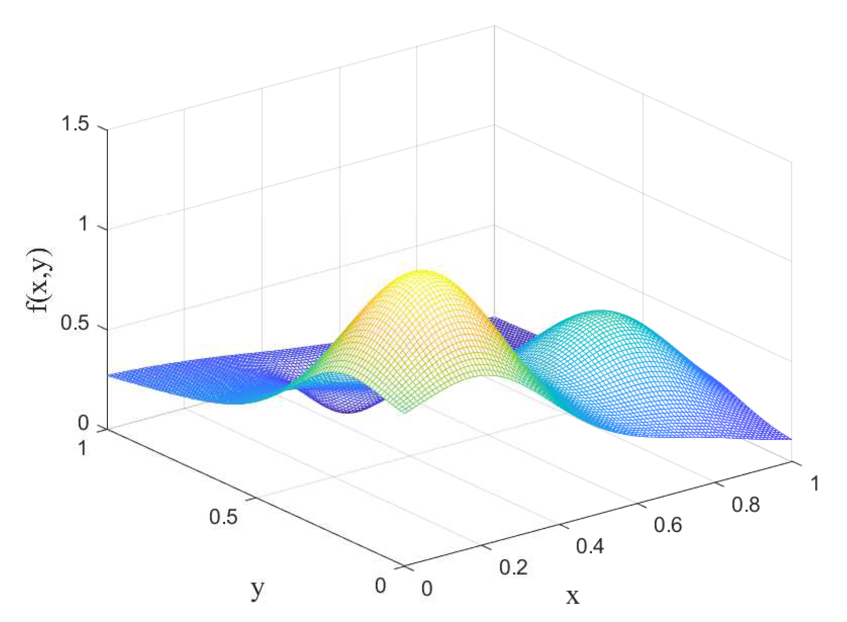
To demonstrate the feasibility and efficiency of our DFO method, we conduct a series of numerical experiments with it. In these experiments, in which the default experimental data are sampled from the Franke’s test function, its expression is

$$\begin{array}{cc}\hfill f(x,y)=& \frac{3}{4}exp\left(\frac{{(9x-2)}^2+{(9y-2)}^2}{4}\right)+\frac{3}{4}exp\left(-\frac{{(9x-2)}^2}{49}-\frac{{(9y+1)}^2}{10}\right)\hfill \\ \hfill & -\frac{1}{5}exp\left(-{(9x-4)}^2-{(9y-7)}^2\right)+\frac{1}{2}exp\left(\frac{{(9x-7)}^2+{(9y-3)}^2}{4}\right),\hfill \\ \hfill & (x,y)\in [0,1]\times [0,1].\hfill \end{array}$$

In all experiments, N represents the number of sampling points, and M represents the number of basis functions. Our sampling points and center points are all the quasi-scattered Halton points [3,20] in $(0,1)\times (0,1)$. The default initial value ${\alpha }_0$ of our DFO method equals 1, if there are no additional instructions.

We use the error between the approximation function and the sample value

$$R_2\left({\alpha }^{\ast }\right)=R({\mathbf{c}}^{\ast },{\alpha }^{\ast })=\sum _{i=1}^N{\left(f_i-\sum _{j=1}^M\left(c_j^{\ast }·{\Phi }_j({\mathbf{x}}_i;{\alpha }^{\ast })\right)\right)}^2$$

(8)

to measure the shape parameter ${\alpha }^{\ast }$, where ${\mathbf{c}}^{\ast }$ is the solution to the classical least squares corresponding to ${\alpha }^{\ast }$. The above formula not only measures the shape parameter, but also shows the approximation effect of the approximation function to the sampling function.

All experiments were implemented on a CPU with Intel Core i7-8700 and with a main frequency of 3.20 GHz. The programming language which we use is Matlab R2019a.

We have opened the sample point sets and center point sets of each experiment, so that the interested readers can reproduce those experiments. Those data are in the Supplementary Materials.

5.1. The Comparison of the DFO Method and the Gauss–Newton Method

In this section, the radial basis function is the thin plate spline function (TPS)

$$\varphi \left(r\right)={\left(\alpha r\right)}^2·ln\left(\alpha r\right),\alpha >0.$$

As mentioned in Section 3, if M is relatively large, obtaining the objective function $R_2\left(\alpha \right)$ of problem (3) is difficult. If M is particularly large, the computational cost of obtaining the expression and derivative of $R_2\left(\alpha \right)$ can be higher than that of solving problem (3). Hence, the Gauss–Newton method is used to solve problem (2), and the DFO method is used to solve problem (3) in this section. Although the problems are solved differently, the Formula (8) can be used to measure the shape parameters in these two ways.

The initial value of the Gauss–Newton method is $({\mathbf{c}}_0,{\alpha }_0)$, here ${\mathbf{c}}_0={\alpha }_0\ast {(1,\dots ,1)}^T$.

5.1.1. The Convergence Comparison

The classical Gauss–Newton method is a method with local convergence. It can converge quickly when the initial point is near the critical point. In addition, our DFO method is a trust-region method. Its convergence rate is theoretically higher than that of the line search method. Hence, we first compare the convergence between the Gauss–Newton method and the DFO method.

In this experiment, $N=5000$, and M takes $50,60,70,$ and $80$, respectively. At first, we set ${\alpha }_0=1$. The results of the two methods in these cases are shown in

Table 1. The results of the Gauss–Newton method and the DFO method on different M values with ${\alpha }_0=1$.

${\mathit{\alpha }}_0=1$		M	50	60	70	80
	Method
$R_2\left({\alpha }^{\ast }\right)$	DFO		0.2307	0.1812	0.1156	0.0928
	Gauss-Newton		0.3156	0.2540	0.1910	0.1072
${\alpha }^{\ast }$	DFO		0.0350	0.0840	0.3971	0.4590
	Gauss-Newton		0.9489	0.9338	0.9215	0.9271

.

The results in Table 1 indicate that ${\alpha }^{\ast }$ obtained by the two methods can be different in the same case. According to the size of $R_2\left({\alpha }^{\ast }\right)$, ${\alpha }^{\ast }$ obtained by the DFO method is more likely to be the optimal shape parameter than that obtained by the Gauss–Newton method. In order to further understand the reason for the result, we use a numerical method to draw the image of $R_2\left(\alpha \right)$ for the case of $M=50$ around two ${\alpha }^{\ast }$s obtained by the two methods in Figure 1.

In Figure 1, the red asterisk represents the ${\alpha }^{\ast }$ obtained by the Gauss–Newton method, and the red circle represents the ${\alpha }^{\ast }$ obtained by the DFO method. We can find that, beginning with ${\alpha }_0=1$, the DFO method can “climb” over a maximum to a minimum on the left, but the Gauss–Newton method can only reach a minimum near the initial value.

We then set ${\alpha }_0=0.5$. The results of the two methods are shown in

Table 2. The results of the Gauss–Newton method and the DFO method on different M values with ${\alpha }_0=0.5$.

${\mathit{\alpha }}_0=1$		M	50	60	70	80
	Method
$R_2\left({\alpha }^{\ast }\right)$	DFO		0.2307	0.1812	0.1160	0.0928
	Gauss-Newton		0.2307	0.1812	0.1160	0.092
${\alpha }^{\ast }$	DFO		0.0350	0.0840	0.3971	0.4590
	Gauss-Newton		0.0350	0.0840	0.3971	0.4590

.

According to Table 2, the results of DFO are almost identical to those of Gauss–Newton. Comparing the results in Table 2 with those in Table 1, the DFO method can achieve the same minimum point beginning with two different initial values. This shows that our DFO method is independent of the initial value selection, while the Gauss–Newton method depends on the initial value.

5.1.2. The Comparison of Computational Efficiency

At first, we set ${\alpha }_0=1$. In order to compare the computational efficiency of the DFO method with that of the Gauss–Newton method, we list their computational times in

Table 3. The comparison of computational time (unit:s) with ${\alpha }_0=1$.

${\mathit{\alpha }}_0=1$		M	10	20	30	40
	Method
t	DFO		0.3824	0.7489	0.8911	1.2423
	Gauss-Newton		0.2628	0.6813	5.3983	2.1273
${\alpha }^{\ast }$	the two methods		0.6073	0.6027	0.2354	0.4456

, when the ${\alpha }^{\ast }$s obtained by the two methods are almost the same. In this experiment, $N=5000$, but M takes $10,20,30$, and $40$, respectively.

The results in Table 3 indicate that, when M is small, the Gauss–Newton method takes less time than the DFO method. However, with the increase of M, the computational time of the DFO method is significantly lower than that of the Gauss–Newton method. Such results are predictable. The problem that the Gauss–Newton method solves is $(M+1)$-dimensional, but the problem that the DFO method solves is one-dimensional. This shows that our dimensional reduction is meaningful.

Thus, we set ${\alpha }_0=0.5$. The initial value is nearer to the ${\alpha }^{\ast }$ in Table 3. We list their computational times in

Table 4. The comparison of computational time (unit:s) with ${\alpha }_0=1$.

${\mathit{\alpha }}_0=1$		M	10	20	30	40
	Method
t	DFO		0.3117	0.7575	0.9185	1.2580
	Gauss–Newton		0.3346	9.7267	1.3497	1.5833
${\alpha }^{\ast }$	the two methods		0.6073	0.6027	0.2354	0.4456

.

Comparing the results in Table 4 with those in Table 3, the computational time of DFO is hardly affected by the initial value, but the computational time of Gauss–Newton is heavily affected by the initial value. The efficiency of the DFO method is less dependent on the initial value.

According to Table 4, the nearer initial value can not make the Gauss–Newton faster than DFO. Combining these results with those in Table 3, we conclude that, when M is large, the computational efficiency of the DFO method is higher than that of the Gauss–Newton method.

Remark 4.

Ideally, we should use the Gauss–Newton method to solve problem (3) in order to make a comparison with the DFO method. However, obtaining the expression and derivatives of $R_2\left(\alpha \right)$ is difficult. The time of obtaining $R_2\left(\alpha \right)$ and $R_2^{\prime }\left(\alpha \right)$ is longer than the time shown in Table 3. Hence, we choose to use the Gauss–Newton method to solve problem (2) instead of problem (3).

5.2. The Results of the DFO Method with a Larger Amount of Data

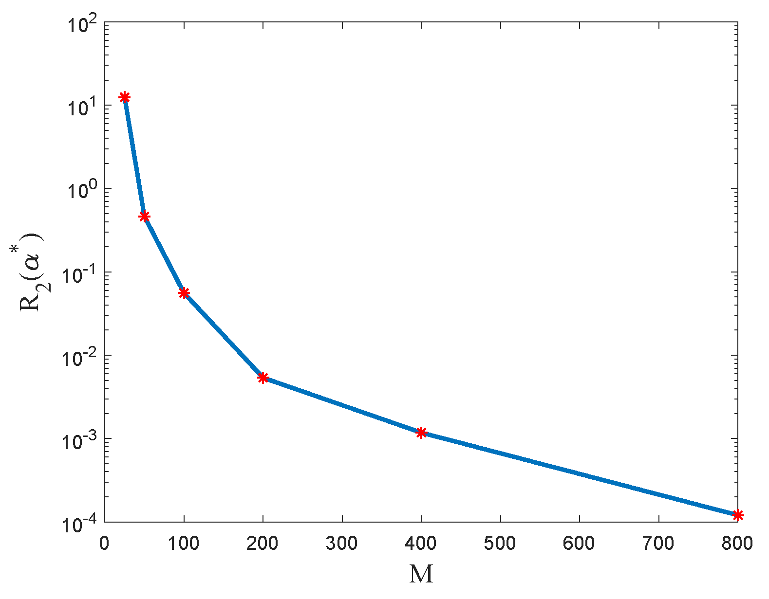
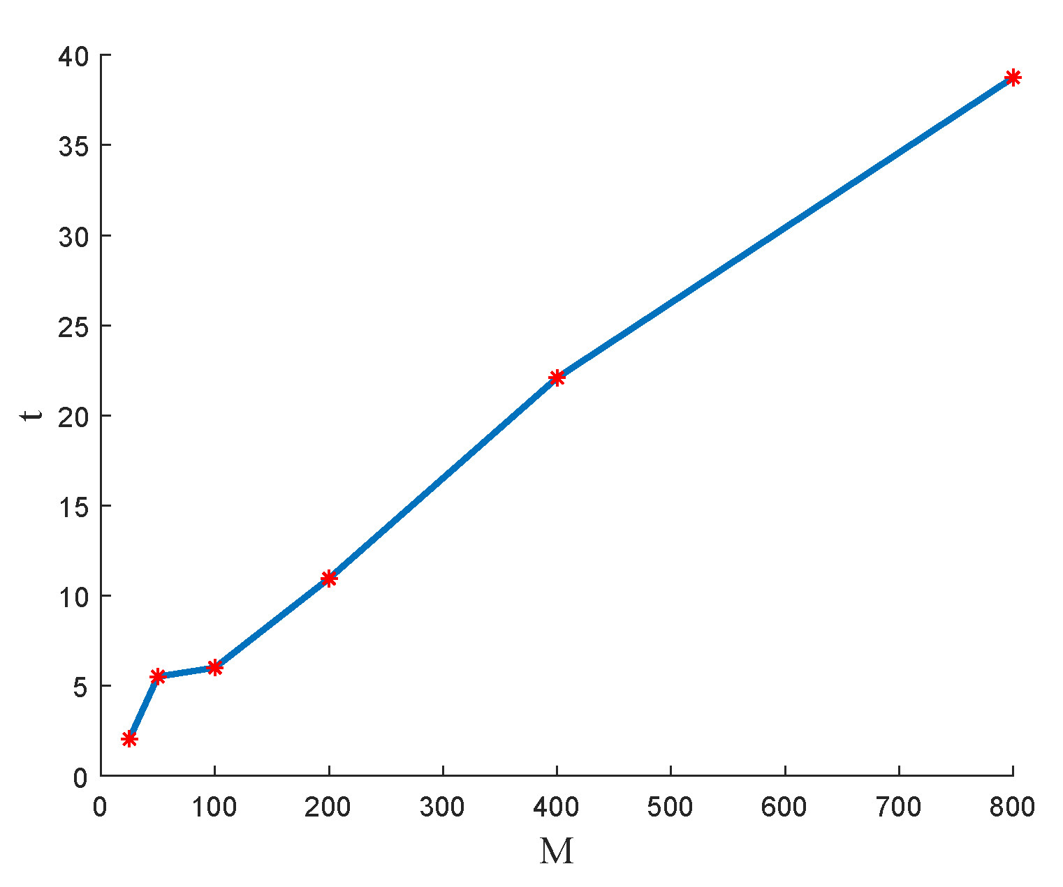
In practice, we often need to approximate large-scale data and use a large number of bases in order to obtain better approximation results. Namely, both N and M are large in general. Hence, we test the DFO method with larger N and M. The RBF is still the TPS function. $N=10,000$ and M takes $25,50,100,200,400$, and 800, respectively. Just like in the previous experiment, we use $R_2\left({\alpha }^{\ast }\right)$ to show the approximation effect. In this experiment, we introduce a graph of $R_2\left({\alpha }^{\ast }\right)$ and a graph of the computational time of the DFO method in relation to M.

Figure 2 shows the relationship between the error $R_2\left({\alpha }^{\ast }\right)$ and M. Figure 3 shows the relationship between the computational time and M.

Figure 2 indicates that, for the same sampling data, the error $R_2\left({\alpha }^{\ast }\right)$ decreases rapidly with the increase of M. In other words, the RBF least squares with a large M and our optimal shape parameter can achieve an excellent approximation. Figure 3 indicates that the relationship between the computational time and M is approximately linear. Hence, the DFO method and our optimal shape parameter are suitable for the case of a large M.

5.3. The Comparison of Results on Different Radial Bases

In order to compare the results on different radial bases adequately, we conduct experiments in two cases. Just like in the previous experiment, we use $R_2\left({\alpha }^{\ast }\right)$ to show the approximation effect. At first, we compare $R_2\left({\alpha }^{\ast }\right)$ and the computational time on different radial bases under two sizes of sampling datasets. Secondly, we add some new test functions and show the results of different radial bases.

Although there are many kinds of RBFs at present, our experiment is only carried out under four commonly used kinds. The four kinds of RBFs are shown in

Table 5. The four kinds of RBFs.

RBF	$\mathit{\varphi }\left(\mathit{r}\right)$	Domain of Definition
Thin plate spline (TPS)	${\left(\alpha r\right)}^2\ast ln\left(\alpha r\right)$	$\alpha >0$
Multi-Quadric (MQ)	${(r^2+{\alpha }^2)}^{\frac{1}{2}}$	$\alpha >0$
Inverse-Quadric (IQ)	$\frac{1}{{(r^2+{\alpha }^2)}^{\frac{1}{2}}}$	$\alpha >0$
CS-RBF (${\varphi }_{3,1}\left(r\right)$)	${(1-\alpha r)}_{+}^4(4\alpha r+1)$	$\alpha >0$

.

We compare the approximation effects and computational time of the DFO method with these basis functions in every experiment.

5.3.1. The Comparison of Two Sizes of Sampling Datasets

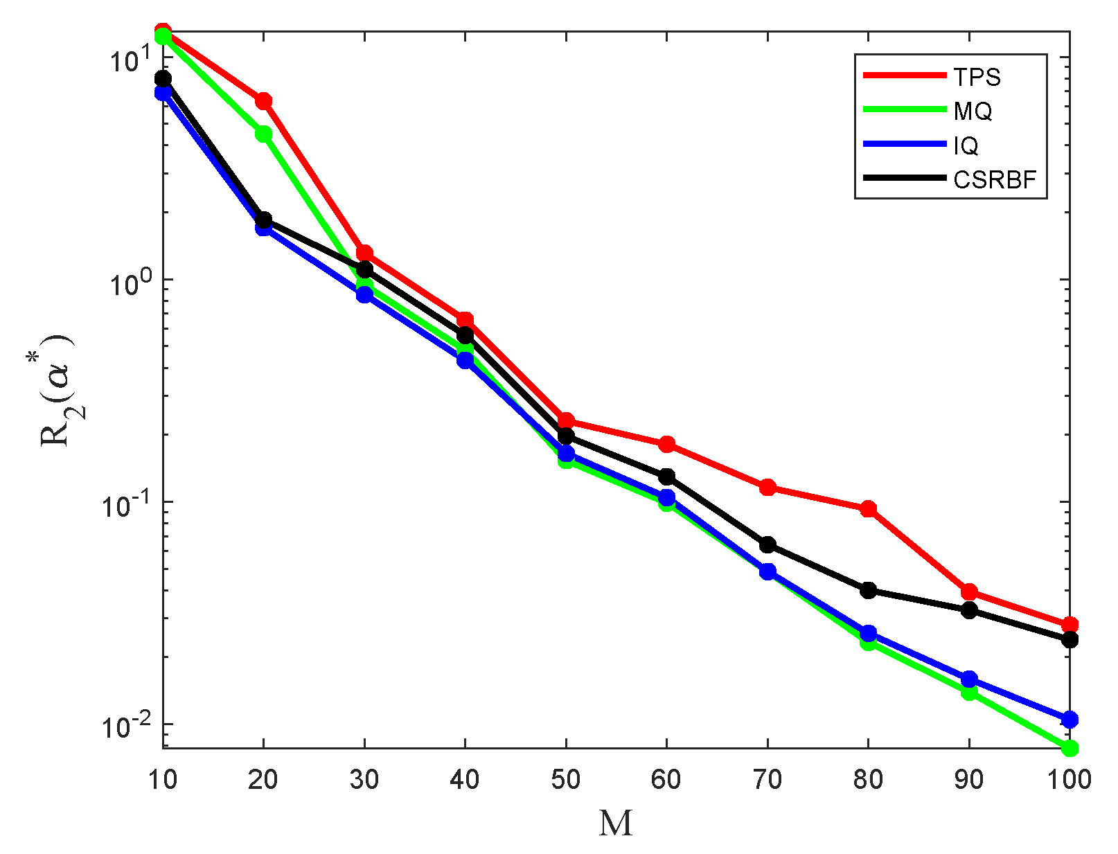
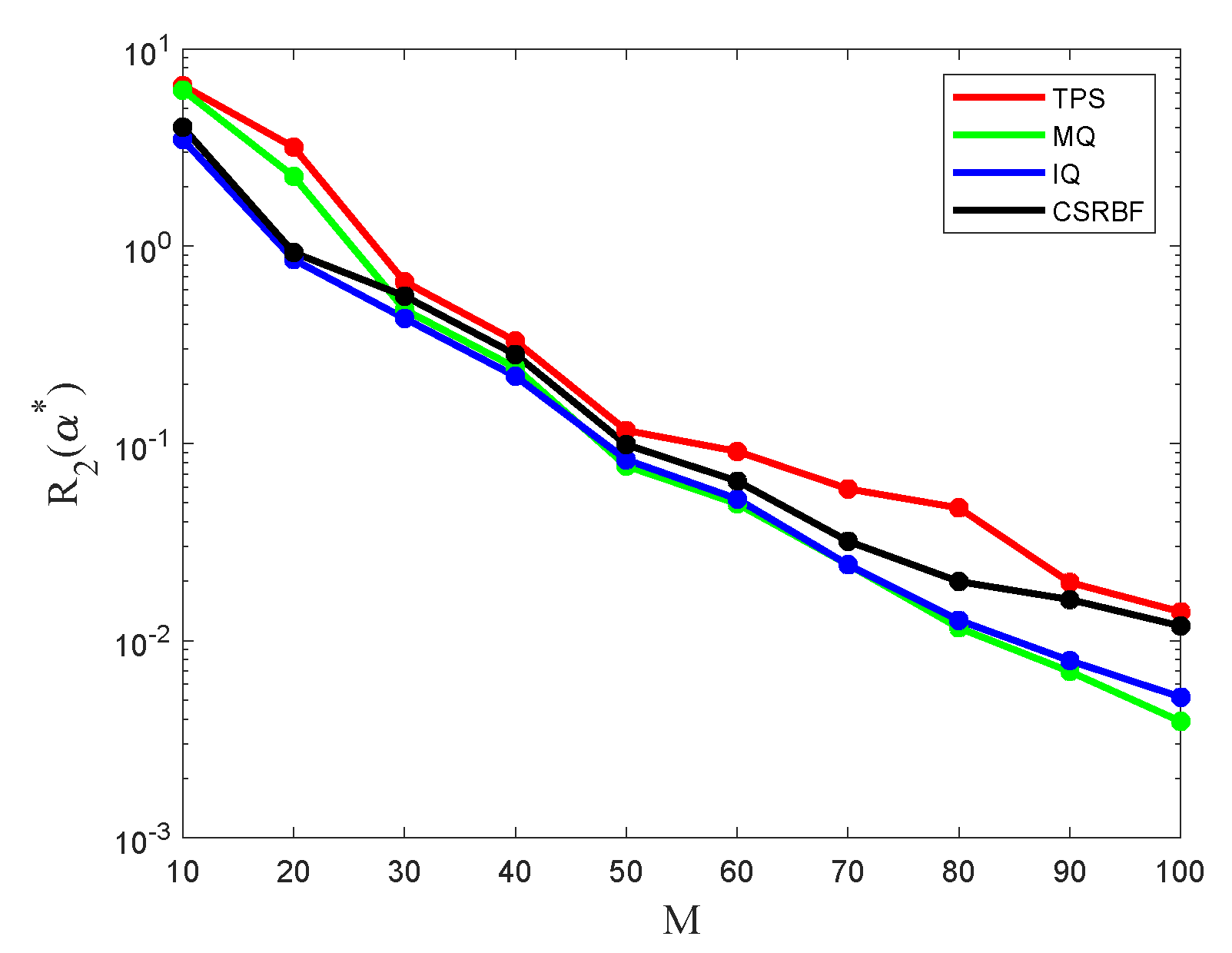
The number of sampling datasets is $N=5000$. They are the quasi-scattered Halton points. The number of center points, M, takes $10,20,\dots ,100$, respectively. Figure 4 shows the relationship between $R_2\left({\alpha }^{\ast }\right)$ and M corresponding to the four kinds of basis functions.

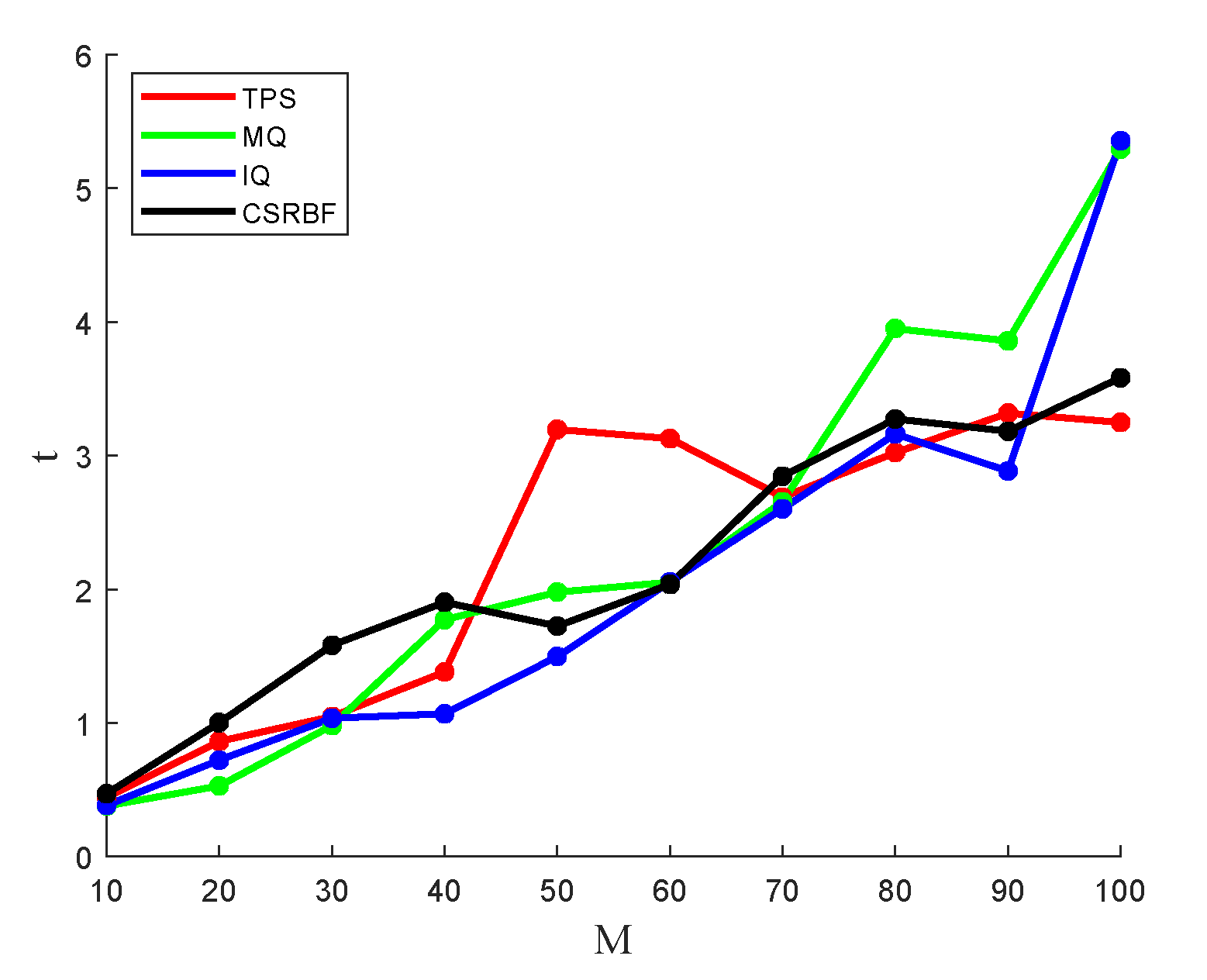
Figure 5 shows the relationship between the computational time and M corresponding to the four kinds of basis functions.

In Figure 4 and Figure 5, the red polyline represents TPS-RBF, the green polyline represents MQ-RBF, the blue polyline represents IQ-RBF, and the black polyline represents CS-RBF [2].

Figure 4 indicates that, whatever the basis function is, $R_2\left({\alpha }^{\ast }\right)$ decreases rapidly with the increase of M. When M is small, the differences among $R_2\left({\alpha }^{\ast }\right)$ of the four basis functions are significant. In this case, the $R_2\left({\alpha }^{\ast }\right)$ of IQ is the lowest, and the $R_2\left({\alpha }^{\ast }\right)$ of TPS is the highest. When M becomes large, all the $R_2\left({\alpha }^{\ast }\right)$ values of the four basis functions decrease rapidly. In most cases, the approximation effect of IQ is the best, and the approximation effect of TPS is the worst.

Figure 5 indicates that, when M is small, the differences among the computational time of the four kinds of basis functions are not significant. As M increases, the differences in the computational time become obvious. In most cases, the computational time of IQ is the lowest. However, if $M=100$, the computational time of IQ becomes relatively high.

We then reduce the N from 5000 to 2500, and others are unchanged. The results of this experiment are shown in Figure 6 and Figure 7.

If we compare the results in Figure 6 and Figure 7 with those in Figure 4 and Figure 5, we can find that the conclusions are similar. The performance of IQ in our experiments is excellent, which is compared with the other three kinds of basis functions.

Based on the above analysis, we find that the performance of IQ is the best in the four kinds of RBFs. Hence, we recommend IQ-RBF for the high-precision problems.

5.3.2. The Comparison of the Four New Test Functions

In this section, we add the following four new test functions,

$$\begin{array}{cc}\hfill g_1(x,y)=& \frac{tanh(9y-9x)+1}{9},\hfill \\ \hfill g_2(x,y)=& \frac{1.25+cos\left(5.4y\right)}{6+6{(3x-1)}^2},\hfill \\ \hfill g_3(x,y)=& \frac{1}{3}exp\left(-5.0625({(x-0.5)}^2+{(y-0.5)}^2)\right),\hfill \\ \hfill g_4(x,y)=& \frac{1}{3}exp\left(-20.25({(x-0.5)}^2+{(y-0.5)}^2)\right).\hfill \end{array}$$

They are functions commonly used to test the performance of the RBF approximation. The four test functions are only used in this section.

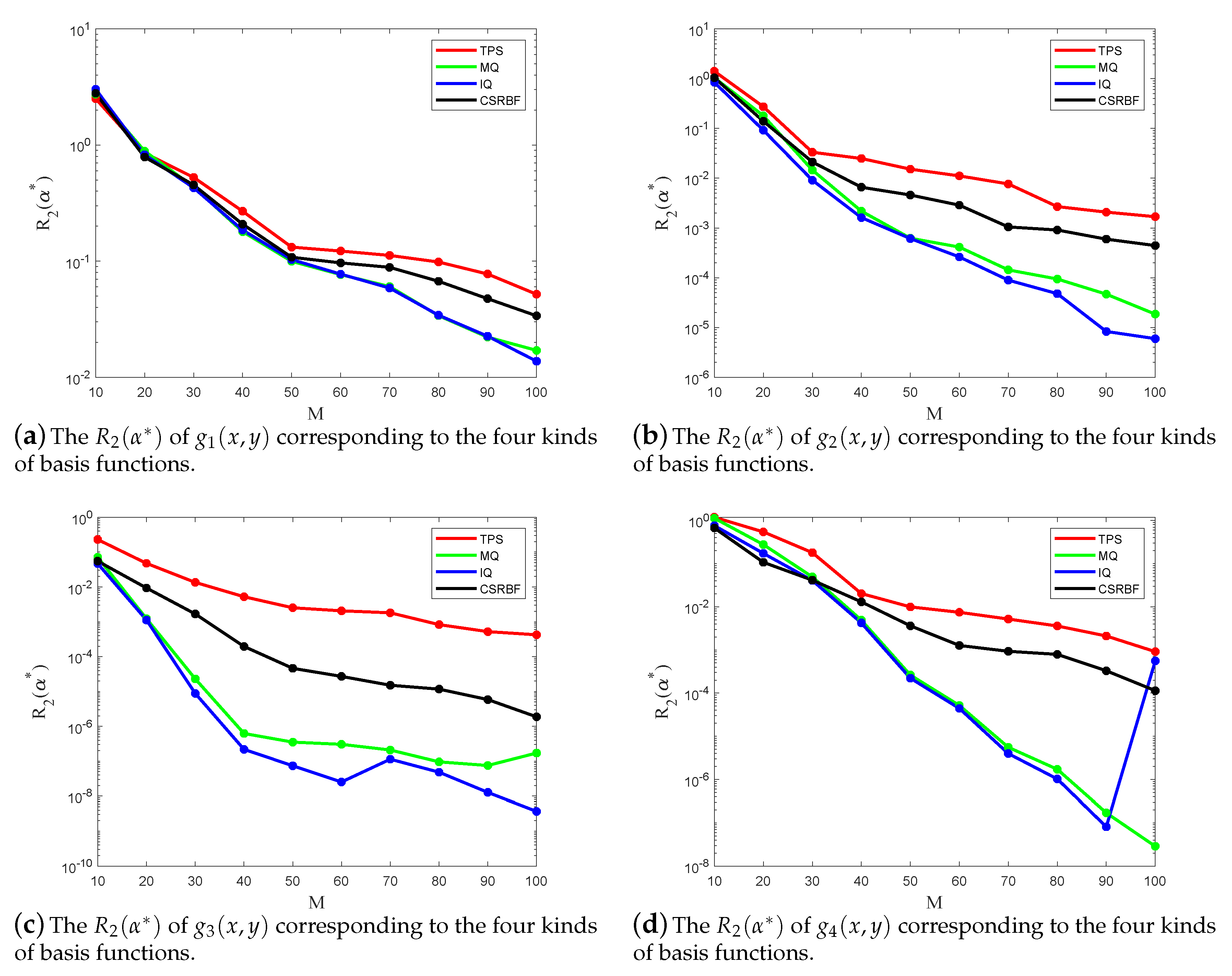
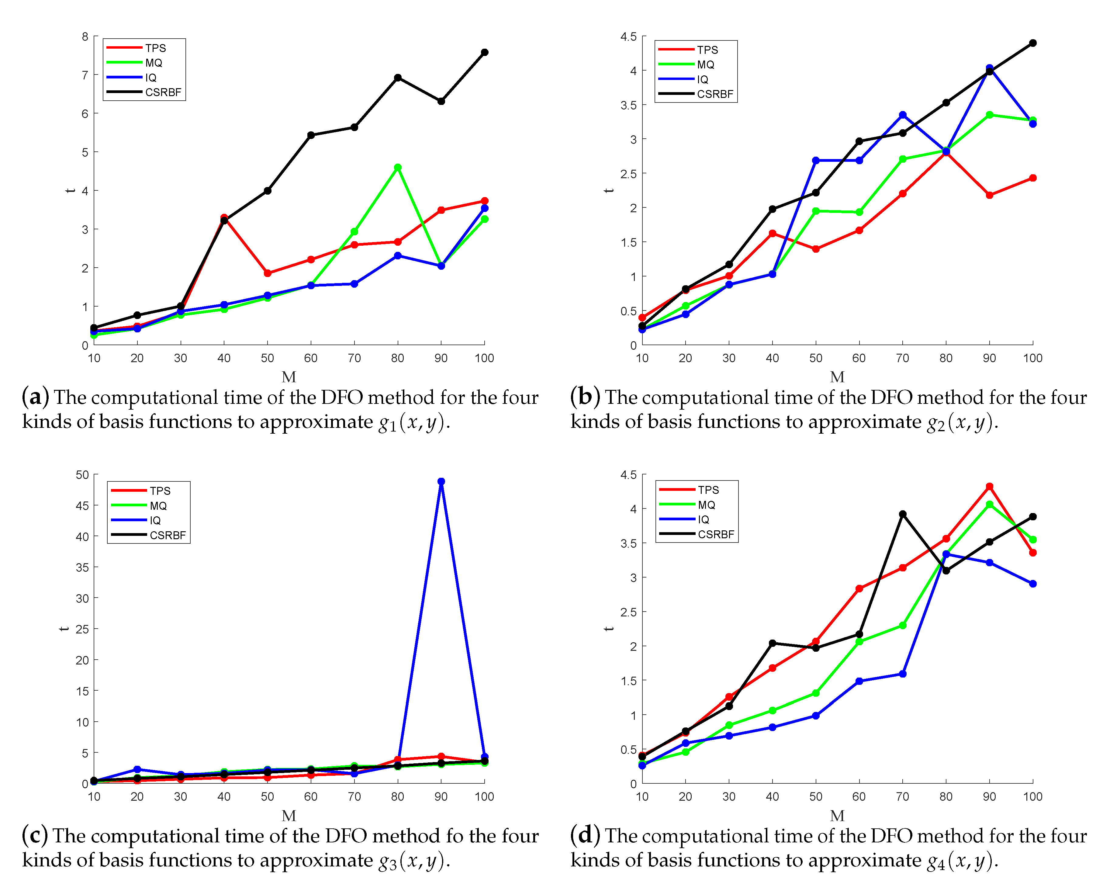
In this section, the number of sampling datasets is always $N=5000$, and M takes $10,20,\dots ,100$, respectively. The approximation effects and computational times of the DFO method are shown in Figure 8 and Figure 9, respectively. Each of the two figures has four subfigures corresponding to the four test functions.

Figure 8 shows that the performances of MQ and IQ are better than that of TPS and CSRBF. In most cases, the $R_2\left({\alpha }^{\ast }\right)$ of IQ is the lowest among the four kinds of basis functions. However, as shown in Figure 8d, when $M=100$, the $R_2\left({\alpha }^{\ast }\right)$ of $g_4(x,y)$ based on IQ indicates that the DFO method may have failed.

Figure 9c shows that there is a special case in which the DFO method may take longer than expected. In most cases, the computational time of every basis function is low and the relationship between the computational time and M is approximately linear, though we cannot prove this in theory yet. According to Figure 9, CSRBF spends the longest time in most cases, IQ has a good performance with respect to $g_1(x,y)$ and $g_4(x,y)$, and TPS has a good performance with respect to $g_2(x,y)$ and $g_3(x,y)$.

Combining the results of Section 5.3.1 with those of this section, although there may be some unexpected results with respect to IQ-RBF on the approximation effect and computational time, IQ-RBF is the most recommended of the four basis functions in most cases.

5.4. Curved Surface Fitting

In this section, we present the application of the RBF least squares with the optimal shape parameter to the surface fitting of the simulated data and real data. We compare the approximation effect of the RBF least squares with that of the polynomial least squares with the same dimension on the simulated data.

5.4.1. Curved Surface Fitting on Simulated Data

In this experiment, the simulated data were sampled from Franke’s test function. Figure 10 is the image of Franke’s test function.

We sampled exactly at $N=5000$ points to construct the simulated data, which are used for the least squares approximation with a polynomial basis and IQ-RBF. The polynomial space is selected as a binary polynomial space with a total degree less than or equal to 8. The dimension of the polynomial space is 45. Accordingly, the IQ-RBF approximation space is constructed with $M=45$ basis functions.

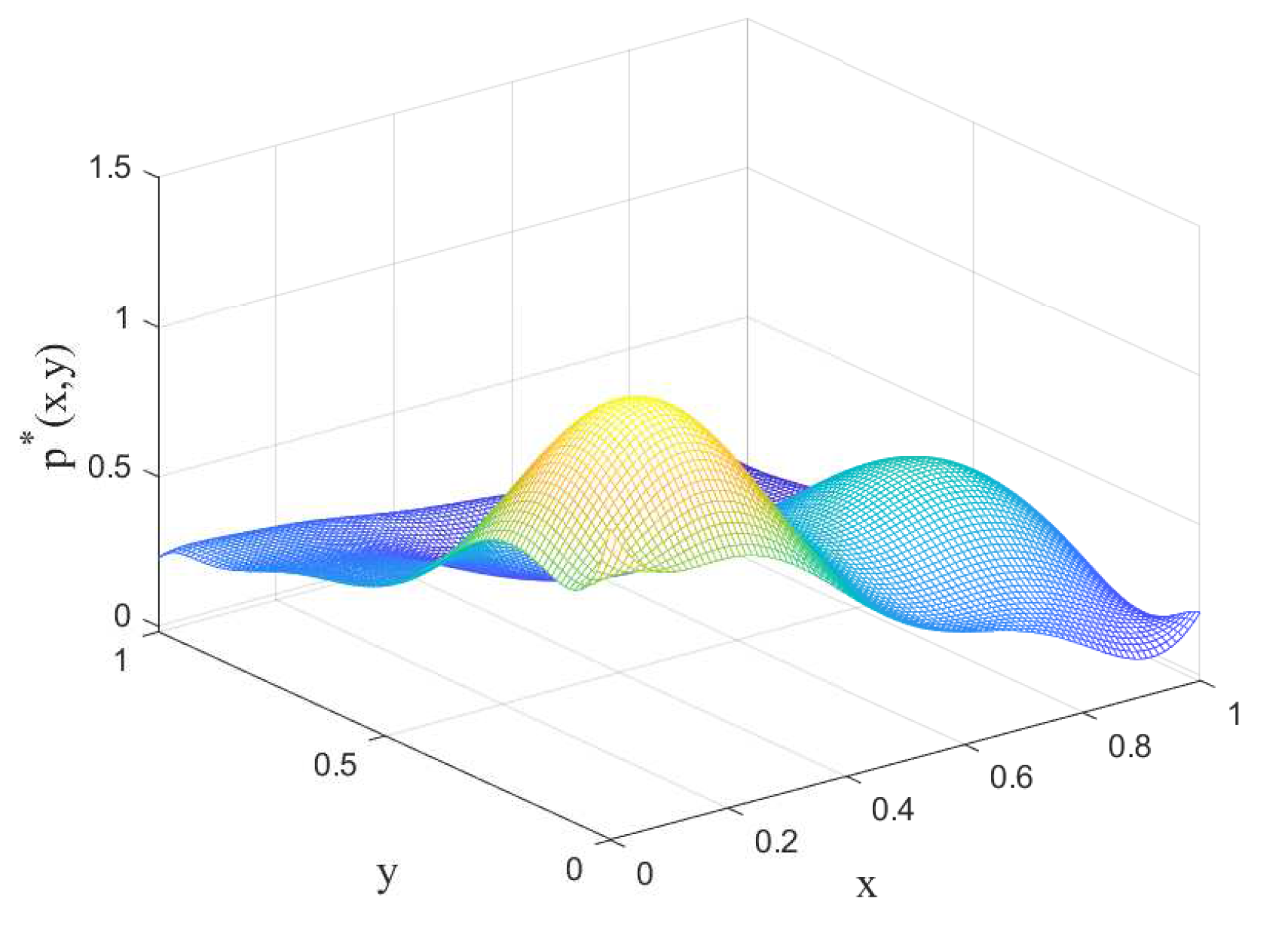
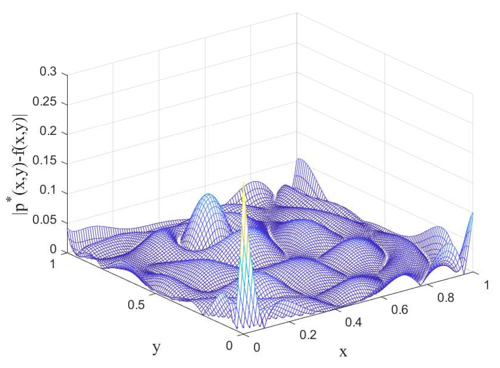
The approximation function of the least squares based on polynomial is $p^{\ast }(x,y)$. The approximation function $p^{\ast }(x,y)$ and the error function $|p^{\ast }(x,y)-f(x,y)|$ on $[0,1]\times [0,1]$ are shown in Figure 11 and Figure 12 respectively.

According to Figure 11 and Figure 12, the error at some points is relatively large, though the approximation function $p^{\ast }(x,y)$ has a certain approximation accuracy to the surface by the simulation data. A comparison between Figure 10 and Figure 11 shows an obvious difference between $p^{\ast }(x,y)$ and $f(x,y)$. In Figure 12, the maximum error is 0.2577, and the average error is 0.0132.

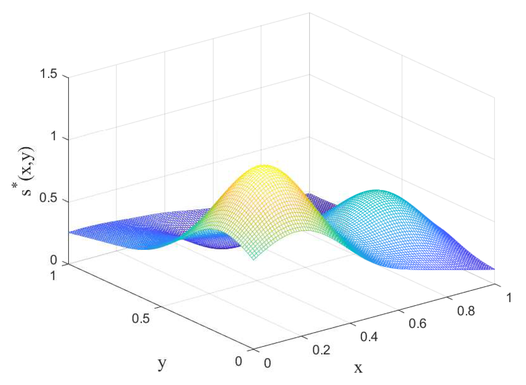
The optimal shape parameter of IQ-RBF with these data is ${\alpha }^{\ast }=0.3047$; the optimal approximation function of the least squares based on IQ-RBF is $s^{\ast }(x,y)$. The approximation function $s^{\ast }(x,y)$ and the error function $|s^{\ast }(x,y)-f(x,y)|$ on $[0,1]\times [0,1]$ are shown in Figure 13 and Figure 14, respectively.

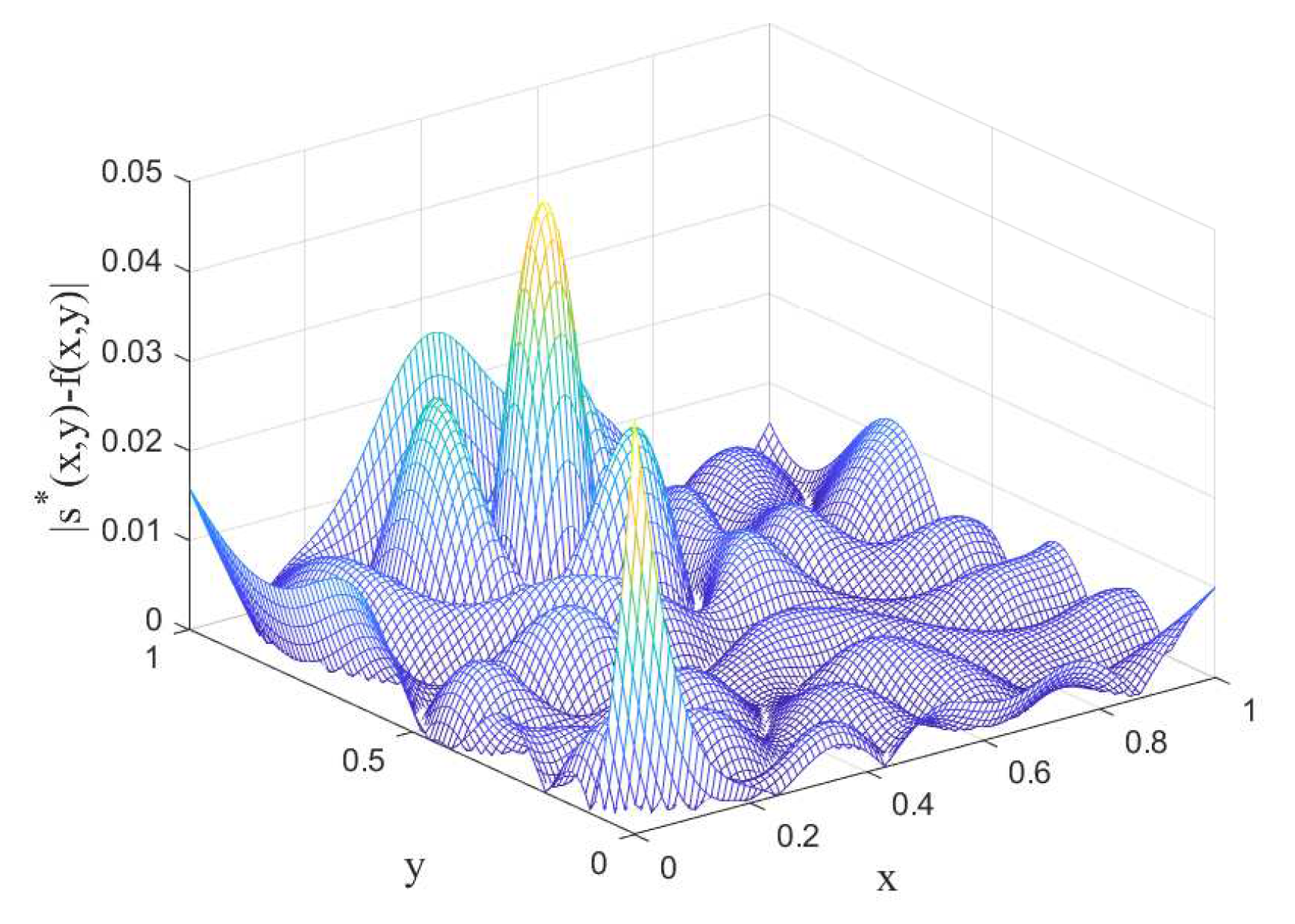
Figure 10, Figure 11 and Figure 13 show that $s^{\ast }(x,y)$ is closer to $f(x,y)$ than $p^{\ast }(x,y)$. Figure 14 indicates that the error $|s^{\ast }(x,y)-f(x,y)|$ oscillates violently, but the numbers are small. In Figure 14, the maximum error is 0.0463, and the average error is 0.0049.

By comparing Figure 12 with Figure 14, we can find that the maximum error and average error of $s^{\ast }(x,y)$ are lower than those of $p^{\ast }(x,y)$.

Table 6. The errors of least squares approximation based on different polynomial spaces and RBF space with the same dimension.

Dimension	Polynomial Basis			RBF
	Total Degree	Max Error	Average Error	Max Error	Average Error
28	6	0.2448	0.0266	0.0831	0.0118
36	7	0.1737	0.0187	0.0674	0.0078
45	8	0.2577	0.0132	0.0463	0.0049
55	9	0.1493	0.0105	0.0468	0.0037
66	10	0.1068	0.0069	0.0353	0.0022

shows the errors of the least squares approximation for the binary polynomial spaces with a total degree less than or equal to 6–10, respectively. The errors of the IQ-RBF approximation whose approximation space has the same dimension as the corresponding polynomial spaces are also shown in the table.

According to Table 6, the results about the binary polynomial spaces with a total degree less than or equal to 8 appear to be extensive. Therefore, we think that the curved surface fitting by the RBF least squares with the optimal shape parameter is better than that by the least squares based on polynomial bases.

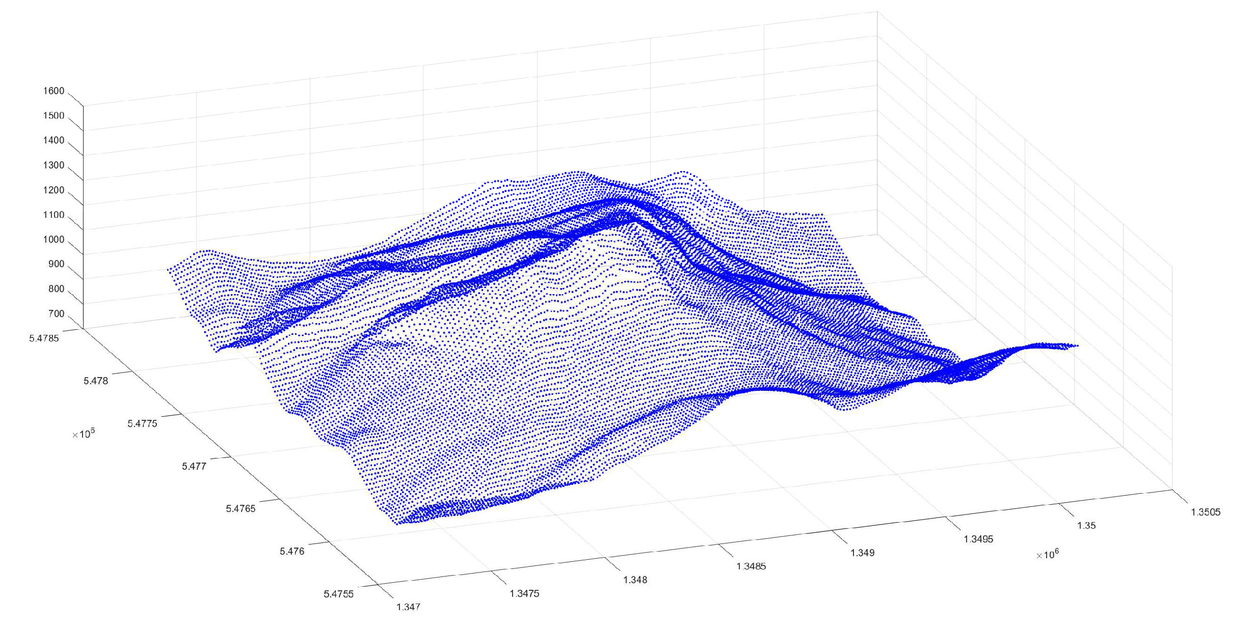
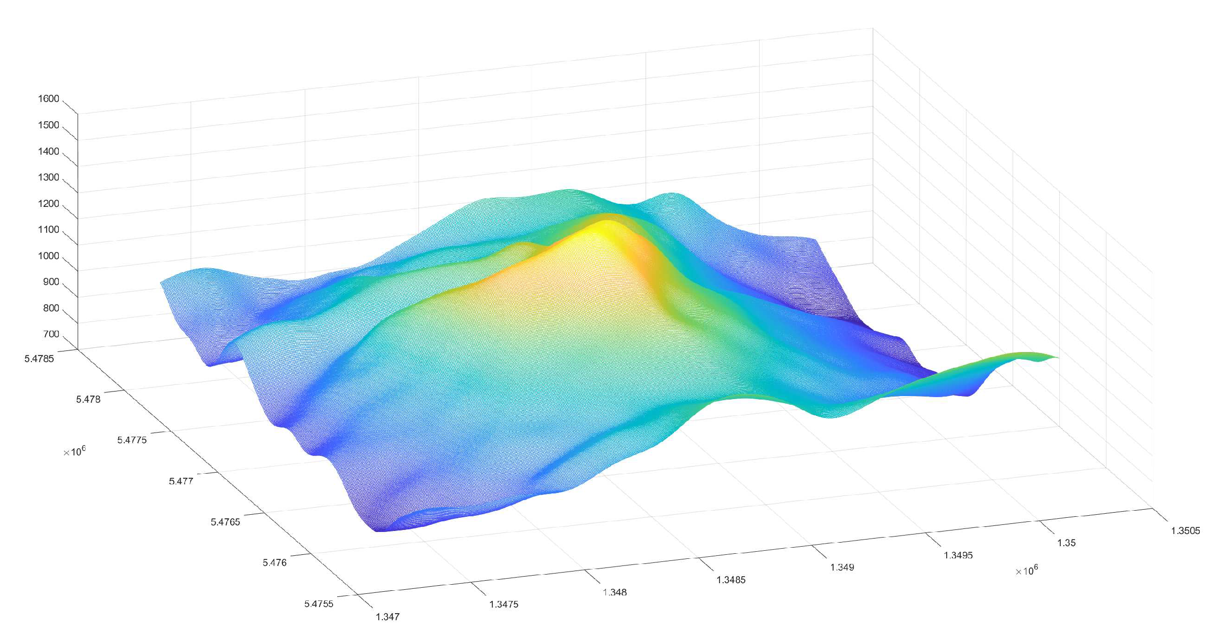
5.4.2. Curved Surface Fitting on Real Data

The real data set is obtained from GPS data of Mount Vel’ký Rozsutec in the Malá Fatra through the online tool GPSVisualizer (http://www.gpsvisualizer.com/elevation). These data have 24,190 points in total and are shown in Figure 15.

We only use IQ-RBF to fit the real data and select the $M=500$ points in the region as the center point to generate the RBF approximation function space. We begin our DFO method with the initial value ${\alpha }_0=1$. In this case, the optimal shape parameter is ${\alpha }^{\ast }=424.8005$, and the fitting surface is shown in Figure 16.

By comparing Figure 15 with Figure 16, we find that the RBF least squares with the optimal shape parameter have a smooth and continuous approximation. The peaks, ridges, and ravines of the mountain are well reconstructed. This approximation is acceptable.

We tabulate the error of RBF least approximation on different shape parameters in

Table 7. The RMSE of the RBF least squares approximation on different shape parameters.

$\mathit{\alpha }$	1	10	100	200	400	${\mathit{\alpha }}^{\ast }=424.8005$	600
RMSE	69.8787	49.4357	10.4753	5.3136	4.0813	4.0787	4.8043

. The error is the famous RMSE (root mean square error).

The initial value is far away from our optimal shape parameter ${\alpha }^{\ast }=424.8005$. The error at the initial value ${\alpha }_0=1$ is very high. The results in Table 7 show that the optimal shape parameter can significantly improve the error, and our DFO method is effective when it begins with a bad initial value.

6. Conclusions

This paper investigates the selection of shape parameters in the RBF least squares. The approximation error of the least squares is used to measure the shape parameter, and we propose a corresponding optimization problem (2) to obtain the optimal shape parameter. In order to reduce the difficulty in solving the problem, an equivalent one-dimensional optimization problem (3) is obtained through variable separation. According to the characteristics of problem (3), we propose to solve it by using the derivative-free optimization method.

Among the various DFO methods, we choose Powell’s UOBYQA method, and we propose our DFO method by combining the characteristics of problem (3) with Powell’s method in Section 4.

We test our method in different cases by numerical experiments. Our method outperforms the classical Gauss–Newton method in the experiments. The performance of our DFO method to solve the least squares approximation based on IQ-RBF is excellent. The surface fitting by the RBF least squares with the optimal shape parameter is better than that by the least squares based on polynomial bases.

The approximation function $s^{\ast }\left(\mathbf{x}\right)$ with the optimal shape parameter can approximate the sampling function more closely than the normal least squares approximation. Hence, the optimal shape parameter is applied to the various applications of least squares. For example, when solving partial differential equations with least squares, we can approximate the exact solution better with the method proposed in Section 4; alternatively, when fitting the surface, we can approximate the sampled surface better by the least squares based on RBF with the optimal shape parameter.

The method used in this paper to define the optimal shape parameter directly implies the generalization that each basis function has an independent shape parameter, which would mean that the problem (2) would become a $2M$-dimensional optimization problem. Such a generalization will undoubtedly improve the approximation effect, but the difficulty of solving problem (2) will further increase. How the $2M$-dimensional nonlinear optimization can be solved efficiently is worth considering.