To Google or Not: Differences on How Online Searches Predict Names and Faces


Abstract
:1. Introduction
2. Materials and Methods
2.1. Participants
2.2. Stimuli
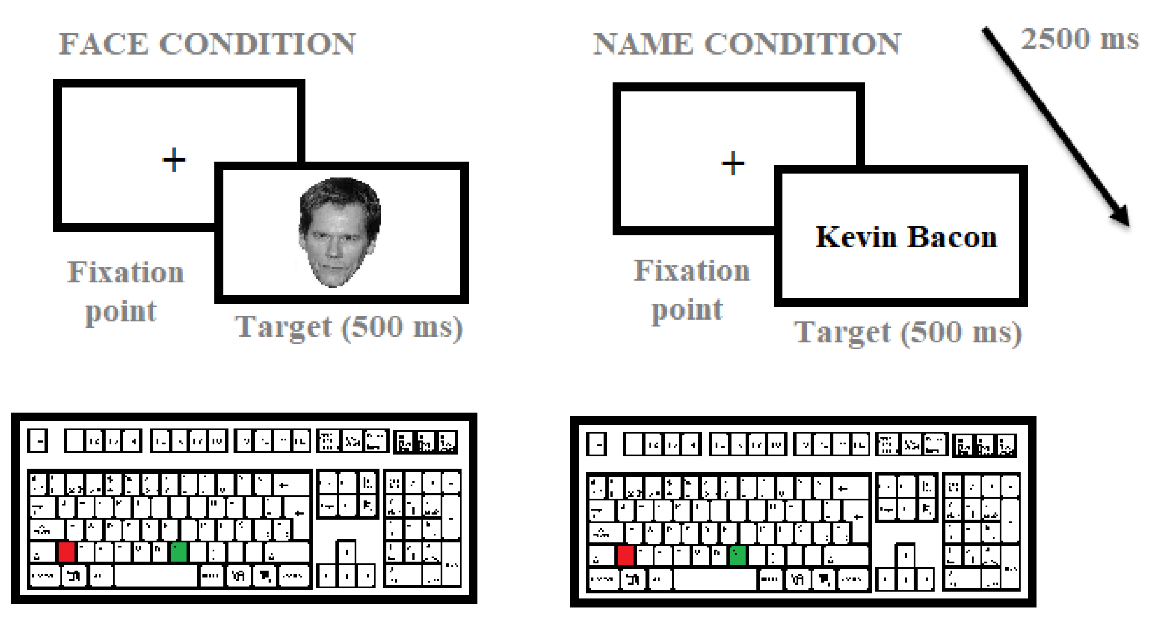
2.3. Procedure
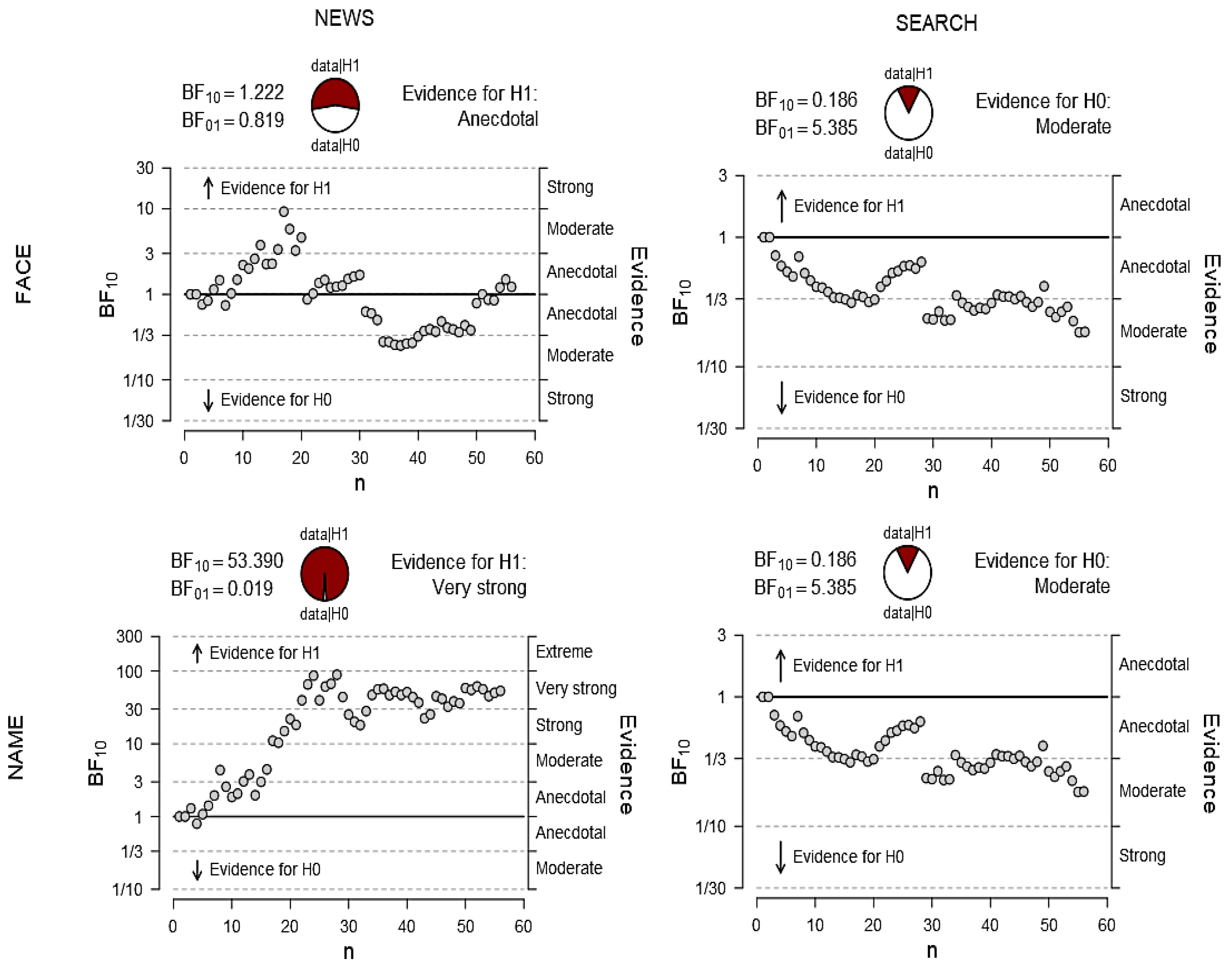
2.4. Data Analysis
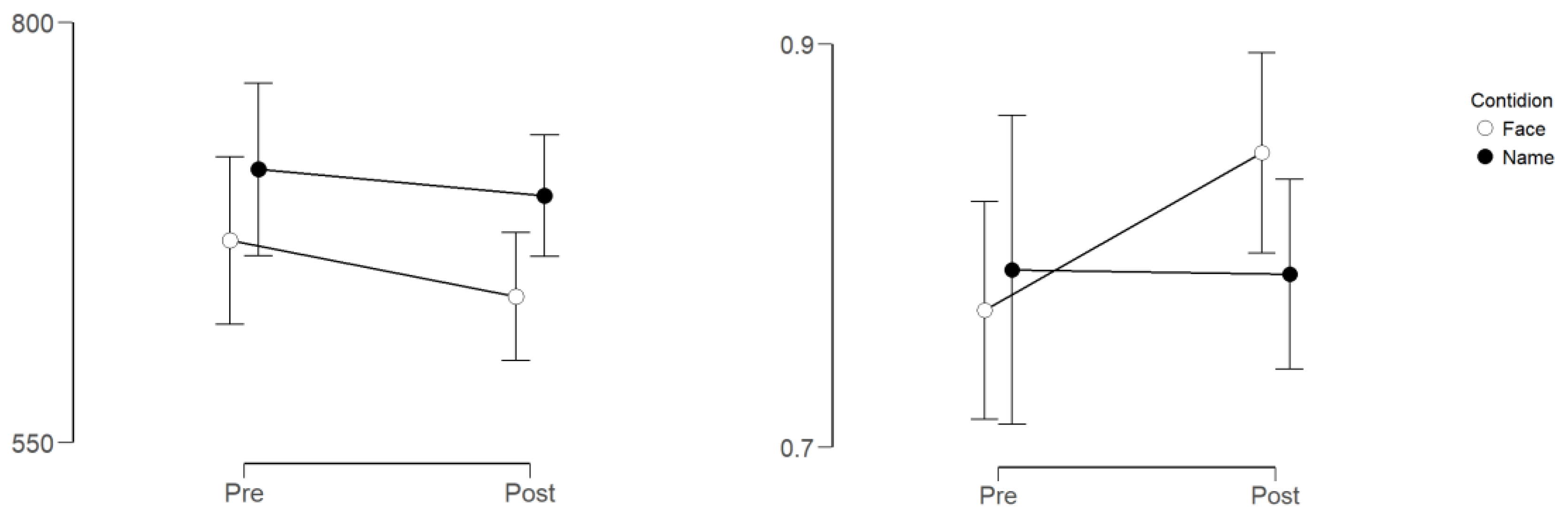
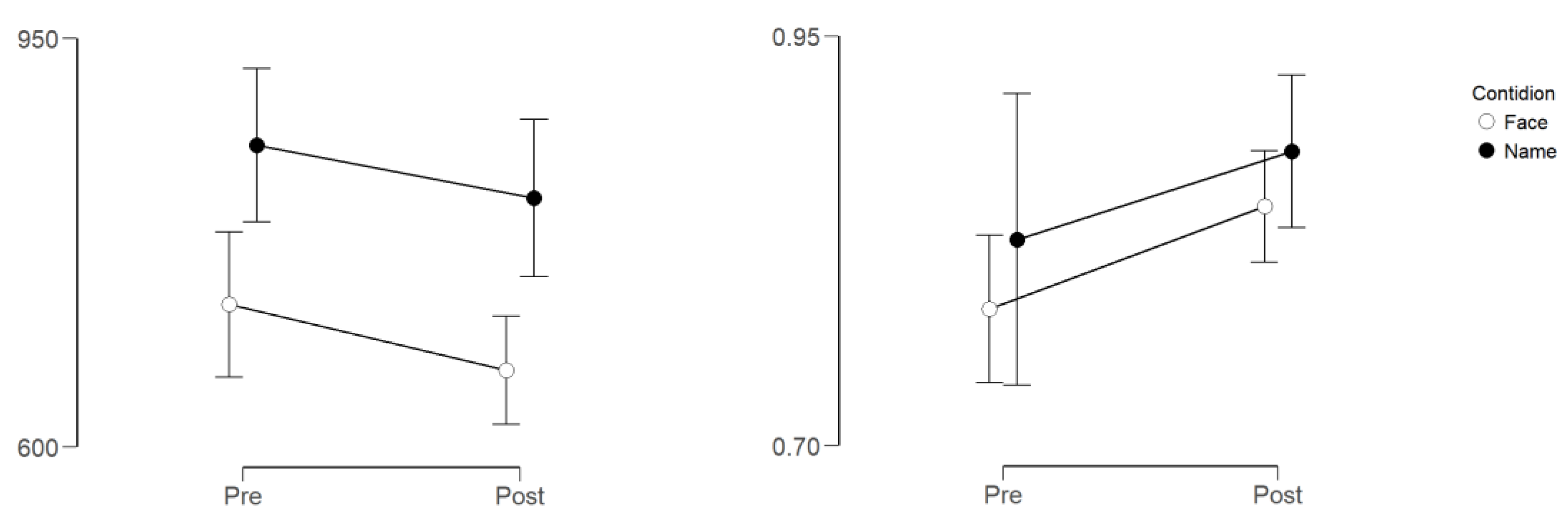
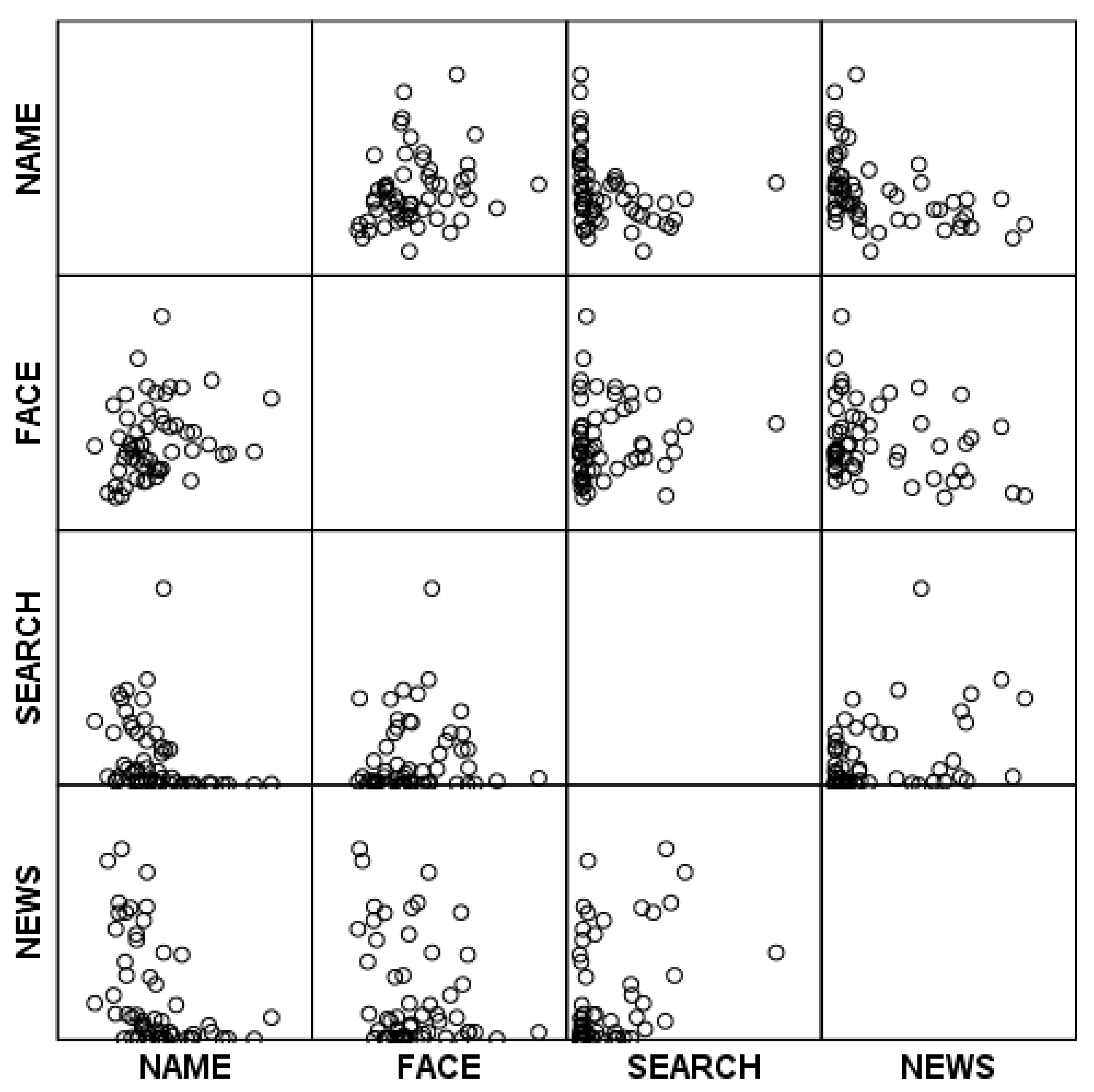
3. Results
4. Discussion
5. Conclusions
Author Contributions
Funding
Acknowledgments
Conflicts of Interest
References
- Dehaene, S.; Cohen, L. The unique role of the visual word form area in reading. Trends Cogn. Sci. 2011, 15, 254–262. [Google Scholar] [CrossRef]
- Griffin, J.W.; Motta-Mena, N.V. Face and Object Recognition. In Encyclopedia of Evolutionary Psychological Science; Shackelford, T.K., Weekes-Shackelford, V.A., Eds.; Springer International Publishing: Cham, Switzerland, 2019; pp. 1–8. ISBN 978-3-319-16999-6. [Google Scholar]
- Moret-Tatay, C.; Lami, A.; Oliveira, C.R.; Beneyto-Arrojo, M.J. The mediational role of distracting stimuli in emotional word recognition. Psicol. Reflex. Crítica 2018, 31, 1. [Google Scholar] [CrossRef] [PubMed] [Green Version]
- Rezlescu, C.; Susilo, T.; Wilmer, J.B.; Caramazza, A. The inversion, part-whole, and composite effects reflect distinct perceptual mechanisms with varied relationships to face recognition. J. Exp. Psychol. Hum. Percept. Perform. 2017, 43, 1961–1973. [Google Scholar] [CrossRef] [PubMed] [Green Version]
- Wegrzyn, M.; Vogt, M.; Kireclioglu, B.; Schneider, J.; Kissler, J. Mapping the emotional face. How individual face parts contribute to successful emotion recognition. PLoS ONE 2017, 12, e0177239. [Google Scholar] [CrossRef] [PubMed] [Green Version]
- Brysbaert, M.; Buchmeier, M.; Conrad, M.; Jacobs, A.M.; Bölte, J.; Böhl, A. The Word Frequency Effect: A Review of Recent Developments and Implications for the Choice of Frequency Estimates in German. Exp. Psychol. 2011, 58, 412–424. [Google Scholar] [CrossRef] [PubMed]
- Gimenes, M.; New, B. Worldlex: Twitter and blog word frequencies for 66 languages. Behav. Res. Methods 2016, 48, 963–972. [Google Scholar] [CrossRef] [PubMed]
- Singer, L.M.; Alexander, P.A. Reading on Paper and Digitally: What the Past Decades of Empirical Research Reveal. Rev. Educ. Res. 2017, 87, 1007–1041. [Google Scholar] [CrossRef]
- Brysbaert, M.; New, B. Moving beyond Kučera and Francis: A critical evaluation of current word frequency norms and the introduction of a new and improved word frequency measure for American English. Behav. Res. Methods 2009, 41, 977–990. [Google Scholar] [CrossRef] [Green Version]
- Moret-Tatay, C.; Gamermann, D.; Murphy, M.; Kuzmičová, A. Just Google It: An Approach on Word Frequencies Based on Online Search Result. J. Gen. Psychol. 2018, 145, 170–182. [Google Scholar] [CrossRef]
- Wang, M.; Hu, G. A Novel Method for Twitter Sentiment Analysis Based on Attentional-Graph Neural Network. Information 2020, 11, 92. [Google Scholar] [CrossRef] [Green Version]
- Rosa, E.; Tapia, J.L.; Perea, M. Contextual diversity facilitates learning new words in the classroom. PLoS ONE 2017, 12, e0179004. [Google Scholar] [CrossRef] [Green Version]
- Pagán, A.; Nation, K. Learning Words Via Reading: Contextual Diversity, Spacing, and Retrieval Effects in Adults. Cogn. Sci. 2019, 43, e12705. [Google Scholar] [CrossRef] [PubMed] [Green Version]
- Balota, D.A.; Yap, M.J.; Hutchison, K.A.; Cortese, M.J.; Kessler, B.; Loftis, B.; Neely, J.H.; Nelson, D.L.; Simpson, G.B.; Treiman, R. The English Lexicon Project. Behav. Res. Methods 2007, 39, 445–459. [Google Scholar] [CrossRef] [PubMed] [Green Version]
- Brysbaert, M.; Keuleers, E.; New, B. Assessing the Usefulness of Google Books’ Word Frequencies for Psycholinguistic Research on Word Processing. Front. Psychol. 2011, 2, 27. [Google Scholar] [CrossRef] [PubMed] [Green Version]
- Sunday, M.A.; Patel, P.A.; Dodd, M.D.; Gauthier, I. Gender and hometown population density interact to predict face recognition ability. Vis. Res. 2019, 163, 14–23. [Google Scholar] [CrossRef] [PubMed]
- Moret-Tatay, C.; Baixauli Fortea, I.; Grau Sevilla, M.D. Challenges and insights for the visual system: Are face and word recognition two sides of the same coin? J. Neurolinguistics 2020, 56, 100941. [Google Scholar] [CrossRef]
- Barragan-Jason, G. How fast is famous face recognition? Front. Psychol. 2012, 3. [Google Scholar] [CrossRef] [Green Version]
- Nanda, S.; Mohanan, N.; Kumari, S.; Mathew, M.; Ramachandran, S.; Pillai, P.G.R.; Kesavadas, C.; Sarma, P.S.; Menon, R.N. Novel Face-Name Paired Associate Learning and Famous Face Recognition in Mild Cognitive Impairment: A Neuropsychological and Brain Volumetric Study. Dement. Geriatr. Cogn. Disord. Extra 2019, 9, 114–128. [Google Scholar] [CrossRef]
- Quaranta, D.; Piccininni, C.; Carlesimo, G.A.; Luzzi, S.; Marra, C.; Papagno, C.; Trojano, L.; Gainotti, G. Recognition disorders for famous faces and voices: A review of the literature and normative data of a new test battery. Neurol. Sci. 2016, 37, 345–352. [Google Scholar] [CrossRef]
- Rizzo, S.; Venneri, A.; Papagno, C. Famous face recognition and naming test: A normative study. Neurol. Sci. 2002, 23, 153–159. [Google Scholar] [CrossRef]
- Nuzzo, R. Scientific method: Statistical errors. Nature 2014, 506, 150–152. [Google Scholar] [CrossRef] [PubMed] [Green Version]
- Suliman, A.; Omarov, B. Applying Bayesian Regularization for Acceleration of Levenberg Marquardt based Neural Network Training. Int. J. Interact. Multimed. Artif. Intell. 2018, 5, 68. [Google Scholar] [CrossRef]
- Vandekerckhove, J.; Rouder, J.N.; Kruschke, J.K. Editorial: Bayesian methods for advancing psychological science. Psychon. Bull. Rev. 2018, 25, 1–4. [Google Scholar] [CrossRef] [Green Version]
- Bernabé-Valero, G.; Blasco-Magraner, J.S.; Moret-Tatay, C. Testing Motivational Theories in Music Education: The Role of Effort and Gratitude. Front. Behav. Neurosci. 2019, 13, 172. [Google Scholar] [CrossRef] [Green Version]
- Moret-Tatay, C.; Beneyto-Arrojo, M.J.; Laborde-Bois, S.C.; Martínez-Rubio, D.; Senent-Capuz, N. Gender, Coping, and Mental Health: A Bayesian Network Model Analysis. Soc. Behav. Personal. Int. J. 2016, 44, 827–835. [Google Scholar] [CrossRef]
- Puga, J.L.; Krzywinski, M.; Altman, N. Bayesian networks. Nat. Methods 2015, 12, 799–800. [Google Scholar] [CrossRef] [PubMed] [Green Version]
- Ruiz-Ruano, A.-M.; López-Puga, J.; Delgado-Morán, J.-J. El componente social de la amenaza híbrida y su detección con modelos bayesianos/ The Social Component of the Hybrid Threat and its Detection with Bayesian Models. URVIO Rev. Latinoam. Estud. Segur. 2019, 57–69. [Google Scholar] [CrossRef]
- Van Doorn, J.; van den Bergh, D.; Bohm, U.; Dablander, F.; Derks, K.; Draws, T.; Etz, A.; Evans, N.J.; Gronau, Q.F.; Hinne, M.; et al. The JASP Guidelines for Conducting and Reporting a Bayesian Analysis. PsyArXiv 2019. [Google Scholar] [CrossRef] [Green Version]
- Moret-Tatay, C.; Gamermann, D.; Navarro-Pardo, E.; de Córdoba Castellá, P.F. ExGUtils: A Python Package for Statistical Analysis With the ex-Gaussian Probability Density. Front. Psychol. 2018, 9, 612. [Google Scholar] [CrossRef] [Green Version]
- Moret-Tatay, C.; Baixauli-Fortea, I.; Sevilla, M.D.G.; Irigaray, T.Q. Can You Identify These Celebrities? A Network Analysis on Differences between Word and Face Recognition. Mathematics 2020, 8, 699. [Google Scholar] [CrossRef]
- Forster, K.I.; Forster, J.C. DMDX: A Windows display program with millisecond accuracy. Behav. Res. Methods Instrum. Comput. 2003, 35, 116–124. [Google Scholar] [CrossRef] [Green Version]
- Moret-Tatay, C.; Leth-Steensen, C.; Irigaray, T.Q.; Argimon, I.I.L.; Gamermann, D.; Abad-Tortosa, D.; Oliveira, C.; Sáiz-Mauleón, B.; Vázquez-Martínez, A.; Navarro-Pardo, E.; et al. The Effect of Corrective Feedback on Performance in Basic Cognitive Tasks: An Analysis of RT Components. Psychol. Belg. 2016, 56, 370–381. [Google Scholar] [CrossRef] [PubMed]
- Fitousi, D. Linking the Ex-Gaussian Parameters to Cognitive Stages: Insights from the Linear Ballistic Accumulator (LBA) Model. Quant. Methods Psychol. 2020, 16, 91–106. [Google Scholar] [CrossRef]
- Balota, D.A.; Cortese, M.J.; Sergent-Marshall, S.D.; Spieler, D.H.; Yap, M.J. Visual Word Recognition of Single-Syllable Words. J. Exp. Psychol. Gen. 2004, 133, 283–316. [Google Scholar] [CrossRef] [PubMed] [Green Version]
- Smith, N.J.; Levy, R. The effect of word predictability on reading time is logarithmic. Cognition 2013, 128, 302–319. [Google Scholar] [CrossRef] [PubMed] [Green Version]
- Susilo, T.; Wright, V.; Tree, J.J.; Duchaine, B. Acquired prosopagnosia without word recognition deficits. Cogn. Neuropsychol. 2015, 32, 321–339. [Google Scholar] [CrossRef] [PubMed] [Green Version]
- Centanni, T.M.; Norton, E.S.; Park, A.; Beach, S.D.; Halverson, K.; Ozernov-Palchik, O.; Gaab, N.; Gabrieli, J.D. Early development of letter specialization in left fusiform is associated with better word reading and smaller fusiform face area. Dev. Sci. 2018, 21, e12658. [Google Scholar] [CrossRef]
- Moret-Tatay, C.; Baixauli-Fortea, I.; Grau-Sevilla, M.D. Profiles on the Orientation Discrimination Processing of Human Faces. Int. J. Environ. Res. Public. Health 2020, 17, 5772. [Google Scholar] [CrossRef]
- Adelman, J.S.; Brown, G.D.A.; Quesada, J.F. Contextual Diversity, Not Word Frequency, Determines Word-Naming and Lexical Decision Times. Psychol. Sci. 2006, 17, 814–823. [Google Scholar] [CrossRef] [Green Version]
- Sunday, M.A.; Dodd, M.D.; Tomarken, A.J.; Gauthier, I. How faces (and cars) may become special. Vis. Res. 2019, 157, 202–212. [Google Scholar] [CrossRef]
- Druică, E.; Vâlsan, C.; Ianole-Călin, R.; Mihail-Papuc, R.; Munteanu, I. Exploring the Link between Academic Dishonesty and Economic Delinquency: A Partial Least Squares Path Modeling Approach. Mathematics 2019, 7, 1241. [Google Scholar] [CrossRef] [Green Version]
- Chen, T.; Qianqian Li, Q.; Jianjun Yang, J.; Guodong Cong, G.; Li, G. Modeling of the Public Opinion Polarization Process with the Considerations of Individual Heterogeneity and Dynamic Conformity. Mathematics 2019, 7, 917. [Google Scholar] [CrossRef] [Green Version]
- Khari, M.; Garg, A.K.; Gonzalez-Crespo, R.; Verdú, E. Gesture Recognition of RGB and RGB-D Static Images Using Convolutional Neural Networks. Int. J. Interact. Multimed. Artif. Intell. 2019, 5, 22. [Google Scholar] [CrossRef]
- Magdin, M.; Prikler, F. Are Instructed Emotional States Suitable for Classification? Demonstration of How They Can Significantly Influence the Classification Result in An Automated Recognition System. Int. J. Interact. Multimed. Artif. Intell. 2019, 5, 141. [Google Scholar] [CrossRef]
- Moaaz, O.; Cesarano, C.; Muhib, A. Some New Oscillation Results for Fourth-Order Neutral Differential Equations. Eur. J. Pure Appl. Math. 2020, 13, 185–199. [Google Scholar] [CrossRef]
- Matsunaga, A.; Fortes, J.A.B. On the Use of Machine Learning to Predict the Time and Resources Consumed by Applications. In Proceedings of the 2010 10th IEEE/ACM International Conference on Cluster, Cloud and Grid Computing, Melbourne, Australia, 17–20 May 2010; pp. 495–504. [Google Scholar]
- Imani, M.; Ghoreishi, S.F.; Allaire, D.; Braga-Neto, U.M. MFBO-SSM: Multi-Fidelity Bayesian Optimization for Fast Inference in State-Space Models. Proc. AAAI Conf. Artif. Intell. 2019, 33, 7858–7865. [Google Scholar] [CrossRef] [Green Version]
- Wang, D.; Hoi, S.C.H.; Wu, P.; Zhu, J.; He, Y.; Miao, C. Learning to name faces: A multimodal learning scheme for search-based face annotation. In Proceedings of the 36th international ACM SIGIR conference on Research and development in information retrieval-SIGIR’ 13, Dublin, Ireland, 28 July–1 August 2013; p. 443. [Google Scholar]


| Face Recognition | Name Recognition | |||||||
|---|---|---|---|---|---|---|---|---|
| Group | Mean | SD | Accuracy | Mean | SD | Accuracy (%) | ||
| Experiment I | Target | PRE | 670.23 | 86.49 | 76 | 712.53 | 108.57 | 78 |
| POST | 636.95 | 77.08 | 84 | 696.93 | 77.62 | 78 | ||
| Distracting | PRE | 721.95 | 117.88 | 78 | 858.33 | 129.55 | 82 | |
| POST | 665.92 | 88.21 | 84 | 813.32 | 106.52 | 88 | ||
| Experiment II | Target | Spain | 634.68 | 88.22 | 80 | 712.96 | 100.68 | 77 |
| USA | 668.59 | 96.43 | 74 | 681.92 | 91.53 | 79 | ||
| Total | 651.64 | 93.40 | 77 | 697.44 | 96.87 | 78 | ||
| Spain | 701.74 | 112.81 | 79 | 843.59 | 137.89 | 81 | ||
| Distracting | USA | 696.42 | 111.18 | 81 | 778.55 | 132.25 | 89 | |
| Total | 699.08 | 111.32 | 80 | 811.07 | 138.17 | 85 | ||
| News | Searches | Face RT | Name RT | Face Hits | Name Hits | |
|---|---|---|---|---|---|---|
| News | 1 | 0.372 ** | −0.271 * | −0.446 ** | 0.305 * | 0.408 ** |
| Searches | 1 | 0.064 | −0.322 * | 0.127 | 0.131 | |
| Face RT | 1 | 0.236 | −0.638 ** | −0.632 ** | ||
| Name RT | 1 | −0.342 ** | −0.496 ** | |||
| Face Hits | 1 | 0.733 ** | ||||
| Name Hits | 1 |
| Face Recognition | Name Recognition | |||||
|---|---|---|---|---|---|---|
| β | p | R2 | β | p | R2 | |
| Search | 0.09 | 0.50 | 0.08 | −0.33 | 0.014 | 0.10 |
| News | −0.37 | 0.03 | 0.13 | −0.46 | <0.01 | 0.20 |
Publisher’s Note: MDPI stays neutral with regard to jurisdictional claims in published maps and institutional affiliations. |
© 2020 by the authors. Licensee MDPI, Basel, Switzerland. This article is an open access article distributed under the terms and conditions of the Creative Commons Attribution (CC BY) license (http://creativecommons.org/licenses/by/4.0/).
Share and Cite
Moret-Tatay, C.; Wester, A.G.; Gamermann, D. To Google or Not: Differences on How Online Searches Predict Names and Faces. Mathematics 2020, 8, 1964. https://doi.org/10.3390/math8111964
Moret-Tatay C, Wester AG, Gamermann D. To Google or Not: Differences on How Online Searches Predict Names and Faces. Mathematics. 2020; 8(11):1964. https://doi.org/10.3390/math8111964
Chicago/Turabian StyleMoret-Tatay, Carmen, Abigail G. Wester, and Daniel Gamermann. 2020. "To Google or Not: Differences on How Online Searches Predict Names and Faces" Mathematics 8, no. 11: 1964. https://doi.org/10.3390/math8111964