A Soft-Rough Set Based Approach for Handling Contextual Sparsity in Context-Aware Video Recommender Systems

Abstract

Context-aware video recommender systems (CAVRS) seek to improve recommendation performance by incorporating contextual features along with the conventional user-item ratings used by video recommender systems. In addition, the selection of influential and relevant contexts has a significant effect on the performance of CAVRS. However, it is not guaranteed that, under the same contextual scenario, all the items are evaluated by users for providing dense contextual ratings. This problem cause contextual sparsity in CAVRS because the influence of each contextual factor in traditional CAVRS assumes the weights of contexts homogeneously for each of the recommendations. Hence, the selection of influencing contexts with minimal conflicts is identified as a potential research challenge. This study aims at resolving the contextual sparsity problem to leverage user interactions at varying contexts with an item in CAVRS. This problem may be investigated by considering a formal approximation of contextual attributes. For the purpose of improving the accuracy of recommendation process, we have proposed a novel contextual information selection process using Soft-Rough Sets. The proposed model will select a minimal set of influencing contexts using a weights assign process by Soft-Rough sets. Moreover, the proposed algorithm has been extensively evaluated using “LDOS-CoMoDa” dataset, and the outcome signifies the accuracy of our approach in handling contextual sparsity by exploiting relevant contextual factors. The proposed model outperforms existing solutions by identifying relevant contexts efficiently based on certainty, strength, and relevancy for effective recommendations.

1. Introduction

Recommender systems (RSs) have been playing a crucial role in helping users for seeking satisfaction and empowering companies through personalization [1]. The online video streaming platforms have led to the overload of information brought about by the abundance of available multimedia choices [2]. Video recommender systems are a subclass of RSs, and these systems are imperative for the effective extraction of relevant multimedia content from a large corpus of data [3]. Typically, the most popular approaches to develop video recommendation algorithms are mainly categorized into three classes. First, the collaborative filtering (CF) method relies on past interactions and user activities by representing users with videos for learning preferences through ratings, by conducting user-video matches in the item space [4]. CF looks for the correlation between user ratings to make predictions. Second, the content-based (CB) method relies upon item description along with the user profiles for exploiting useful information. Lastly, the hybrid approach aims to alleviate the weakness in both techniques by combining them through considering watched videos history and the content related to the videos that are watched by other users with the same interest.

Classical recommender systems work upon a function that contains ratings retrieved through a system or explicitly provided by users. In this manner, two types of entities (user and item) are used to calculate rating function [5]:

$$User\times Item=Rating.$$

(1)

Most of the existing video recommending algorithms do not include contextual information of the users during the recommendation process. Context-aware recommender systems (CARS) improve the accuracy of the recommendation process in different situational scenarios by exploiting contextual factors of the user under which a rating has been given to a particular item [6]:

$$User\times Item\times Context=Rating.$$

(2)

Context is a situation consisting of a set of scenarios under which or due to which action was happening [7]. CARS leverage the accuracy of recommendation by exploiting contextual factors like environment, location, and activities of a user for understanding preferences of that user based on certain circumstances and their effect on user choices for the sake of improving the relevance of possible recommendations with respect to a change in user’s needs [8].

As interesting as it may appear, a variety of contexts and user needs cause difficulty in selecting relevant contextual information for incorporating in CAVRS [9,10]. Similarly, it is essential to select influential and relevant contextual factors of the user for predicting videos accurately, which leads to creating intelligent recommendations [11]. In addition, a statistical model is formulated in most of the extant research work on CAVRS and predictions for recommendations are made with validating the available data by considering that the preference of different contexts during recommendation is similar [12]. Nevertheless, the statistical method has its own limitations and cannot produce better predictions when the data contains uncertainty. This limitation has to be removed for resolving the conflicting situation to improve the context selection process in CAVRS. Therefore, identification of contextual information which is most relevant to the users is a major concern in this regard [13].

In this paper, we address the problem of sparse contexts by handling the conflicting situation during the selection of relevant contextual information. Most of the prior research efforts on CAVRS assume the weights of contexts homogeneous by considering the influence of different contextual factors during the recommendation process similar. It causes a conflicting situation that is a major concern and a unique challenge in CAVRS [13,14]. Hence, the main contribution of our research attempt is the development of a novel methodology to cope with the identification and selection of contexts that are most appropriate and influential to the users for video recommendations.

In order to resolve above-mentioned issues, we propose a Soft-Rough Set based attributes reduction approach by which we can cope contextual sparsity issue by identifying the most suitable contexts that will influence user satisfaction and then incorporate them into contextually aware recommender systems. Our approach Soft-Rough Set based CAVRS (SRS-CaVRS) combines rough sets based formal approximation [15] on soft sets based representation of given contextual attributes in Boolean-valued information systems that is able to perform attributes reduction more efficiently to extract the a reduced set of contexts with minimal contextual factors [16] by alleviating contextual sparsity in context-aware video recommender systems.

Currently, the most effective context-aware video recommendation algorithms are based on a contextual modeling approach that estimates deviation in ratings across different contexts. However, it is not guaranteed that, under the same contextual scenario, all the items are evaluated by users for providing dense contextual ratings, whilst dense ratings are not available for all items in the same contexts because a user usually has different preferences in different contexts. Consequently, some context attributes are more important than others [17].

Our proposed methodology will contribute from the perspective of identifying a set of minimal and influencing contextual factors that are of significance for recommendation results. The contribution of this research work can be useful for handling the contextual sparsity issue in studies that use ratings for contextually aware recommendations of items. It can be used by different studies on online streaming platforms that utilize contextual factors during recommendations [7,10,13,18]. These studies use rating functions for item ranking recommendations. However, users have different preferences of watching videos depending upon the particular contextual scenario. Hence, ratings for all the items may not be available in each of the contextual scenarios. This problem causes contextual sparsity in existing solutions. The results from our proposed methodology depict that selection of a minimal set of influencing contextual factors in which a video is most suitable to recommend will alleviate the contextual sparsity issue in these application domains. Likewise, the proposed methodology and results can also be considered in different domains such as context-aware location recommender systems [19], which recommend locations for visits based upon historical ratings of the past users.

This study is organized as follows: existing research efforts and those related to our work have been discussed in Section 2. Some preliminary concepts essential for comprehending the construction of our scheme have been discussed in Section 3. Subsequently, a formal specification of the proposed approach is presented in Section 4. An illustrative example is presented in Section 5 to demonstrate the applicability of the proposed approach. Experimental setup and discussion on results are provided in Section 6, followed by the conclusions of the paper in Section 7.

2. Literature Review

In this section, we review related research work on the development of CAVRS, along with the context weighting approaches for exploitation of relevant contextual attributes.

2.1. CAVRS Background

The process of contextual information incorporation into recommender systems is classified into three approaches. Figure 1 represents the overall working of each of these approaches.

In Figure 1a, the contextual information is incorporated into the recommender system using a pre-filtering based approach. According to this approach, the contextual information will be employed into the 2d recommender system before ranking of recommendations is computed. Likewise, another approach is given in Figure 1b for the incorporation of contextual factors after the computation of the ranking of recommendation through 2d RS methodology. In this approach, the reduction is performed that reduces the results of the computed ranking according to the given contextual scenario. The most emerging approach of context inclusion, however, is contextual modeling. In this approach, the contextual factors are utilized as a major element during the learning phase. Hence, contextual factors are employed as dimensions for computing rating function in addition to the user and item dimension [6]. The process of contextual modeling is given in Figure 1c.

To improve the recommendation accuracy of typical RSs, CARSs are becoming increasingly important [10]. Context-awareness during recommendations was oriented to pave the way for supporting the recommendation process in a specific contextual situation, which contains three main features, including User, Item, and Context [7]. The idea behind CAVRS is that users with similar preference and the same contextual factors like similar videos.

In CARS, the recommendation process starts with the specification of the initial set of ratings that had either been explicitly provided by the users or implicitly retrieved from the system [9]. Using CARS, if a set of contextual factors contains two attributes: Companion and Time, the prediction function to compute ratings will become $\mu$ (U, {C, T}, I). It can be defined as: [15]:

$${}^{\mu }\stackrel{D}{U}ser\times \left\{Family,Weekend\right\}\times Ite{m}^{:U\times \left\{C,T\right\}\times I\to R}$$

(3)

where U is the user, I represents the items, C and T denotes Companion and Time, respectively, which are the contextual factors of the user for this observation. Moreover, D contains records < User, {Family, Weekend}, Item, Rating > for the user-specified ratings R. Equation (3) depicts that the rating R will be computed for a specific item I rated by user U under a given context of family as companions and weekend as time. The rating function can be expressed as follows:

$$\begin{array}{c}{}^{\mu }User\times \left\{Family,Weekend\right\}\times Ite{m}^{(U,\left\{C,T\right\},I)}=\\ {{}^{{\mu }^{\underset{User\times \left\{Family,Weekend\right\}\times Ite{m}^{}}{D[Companion=C\wedge Time=T](User,Item,Ratings)}}}}^{(U,I),}\\ \forall (U,\{C,T\},I)\in U\times \{C,T\}\times I,\end{array}$$

(4)

where D [Companion = C $\Lambda$ Time = T] (U = User, I = Item, R = Ratings) represents a record of ratings generated through D given in Equation (3). It considers the factors where Companion is associated with a value C and Time with value T, and selecting the value of rating along with the value explicitly for User and Item dimensions. For example, a user John has watched “M1” video in a context where companions are Family and Type of the day is Weekend, and makes a rating of 9. Thus, the rating function will become R (John, {Family, Weekend}, “M1”) = 9 (out of 10). It has been illustrated from this rating that John prefers “M1” movie to watch with family on the weekend [13].

Note that weights and preferences of different contexts during recommendation in current approaches are similar [13,14]. Whilst dense rating is not available for all items in the same contexts because a user usually has different preferences in different contexts. Consequently, some context attributes are more important than other [17]. Nevertheless, several studies suggested to identify a set of influencing contextual factors which are of significance for recommendation results, is a valuable topic for research [12,20,21].

2.2. Selection of Influential Contexts

Aided by the rapid proliferation of context-awareness in recommender systems, several approaches are being proposed to create efficient CARS by selecting relevant contexts that are influential for recommendation results [12]. One of the major problems in typical CARS is determining which contextual features are relevant to influence users’ decisions in a particular situation [13]. As the authors in [19] state, irrelevant contextual features can degrade the prediction accuracy of recommendation by spending unnecessary resources on the acquisition of irrelevant context.

To this end, previous work has utilized several techniques to perform detection of relevant and irrelevant context. The authors in [2] had used a paired t-test and $X^2$ test for the detection of influential contextual features in their database. In [13], the authors proposed an approach to determine relevancy between contextual factors using statistical methods of testing on rating data. Likewise, in [12], the authors conducted a context-relevance assessment by performing a survey to evaluate the influence of a given contextual feature by supposing a particular situation. However, as they state, users rate an item differently in a real and supposed contextual situation, whilst the results also revealed that better accuracy for the detection of relevant contextual feature could be achieved through detection process form the rating data in comparison to the survey for the assessment of users’ opinion. Hence, such techniques are problematic [14].

In [22], the authors demonstrate the significance of incorporating relevant context during the development of context-aware recommender algorithms. The data sparsity problem gets aggravated in CARS due to the use of too many contextual features when user preferences are diluted with contextual attributes [23]. However, the incorporation of a few contextual features lacks the capturing of contextual effects that impair prediction performance. The authors in [24] suggested an interesting approach of utilizing explicit ratings which make the algorithms of context-awareness flexible and lightweight by handling the data sparsity problem. In a practical situation, however, the utilization of explicitly obtained ratings is not an effective approach as there are no specific incentives of users for rating items [17]. Despite the fact that most of the previous research has utilized explicit ratings, the authors in [17] proposed an implicit rating approach utilizing the genre of the videos. Addressing previously mentioned issues, a novel framework proposed by [14] utilizes both explicit and implicit ratings for performing multiple rating predictions based on item neighborhood and user neighborhood.

Nevertheless, prior proposed methodologies used in CARS lack utilization of implicit ratings that are assigned in different contextual situations. In order to handle this issue, several studies [20,21,23,25] suggested the assigning of different weights to contextual features during recommendation. The authors in [20] demonstrate that how to select contextual variables is really a serious problem when contextual features are not diluted in the data. They propose a novel approach of Differential Context Relaxation (DCR), according to which minimal subsets of contextual factors were incorporated in different phases of recommendation algorithms. In some cases, however, DCR increases contextual sparsity by restricting the recommender algorithm to take contexts into account [25]., whilst another approach proposed by the same authors in [26] improves the overall working of CARS in which contextual attributes are weighted. Recently, a study [21] proposed an algorithm that utilizes context based communities for the purpose of reducing the data sparsity problem by a weighted percentile approach. The results obtained proved that the weighted percentile approach outperforms for the identification of relevant and influential contextual information [23].

2.3. Attributes and Dimensionality Reduction

From the perspective of handling contextual sparsity in CAVRS, which gets aggravated due to the use of too many contextual features, the selection of a minimal and relevant set of contexts through an attribute reduction approach is required. Attribute reduction focuses on a minimal subset of conditional attributes such that the reduced set provides the classification with the same quality of approximation as the original conditional attribute set [27]. Through this, we can eliminate redundant conditional attributes from the data sets and preserve the partition. A novel approach based on formal approximation using rough sets was proposed by Huang et al. [15]. Rough Set Theory (RST) deals with the analysis of uncertain information by an attribute reduction approach for data mining and knowledge discovery [28]. However, RST lacks the parameterization property and utilizes formal approximation [29]. Several attempts have already been made for efficient attribute reduction using rough sets, including, fuzzy rough set based attribute reduction, which is useful for dealing with numerical or continuous data sets [28]. Similarly, parallel reduction based RST use for heuristic-based attribute reduction. However, it has high computational complexity due to the incorporation of heuristic-based algorithms [30]. In our case, however, the major concern is context sparsity which causes conflicting situations during relevant context selection process. By getting inspiration from these studies, we hybridize rough sets with soft sets. Hence, the given data will be represented in Boolean-valued information systems through soft sets on which formal approximation using rough sets can be applied for assigning weights and reduction of redundant contextual attributes.

This research work addresses the problem of contextual sparsity in CAVRS through a wider and more generic analysis. We proposed an approach that merges soft sets and rough sets for assigning weights to different contexts in order to exploit relevant contextual features that are influential for predicting recommendation and alleviating data sparsity problem in CAVRS. To the best of our knowledge, the prior work applied contextual feature weighting, however, but did not apply in an efficacious way as compared to the approach we attempted in this research work.

Table 1. Comparative analysis with the existing schemes.

Ref	Solution Type	Influential Contexts	Weighting Process	Minimal Contextual Set
[25]	DCR ${}^a$	✓	×	×
[20]	DCW ${}^b$	✓	×	×
[21]	PSO ${}^c$	×	✓	×
[23]	Weighted Percentile	×	✓	×
SRS-CaVRS${}^d$	Soft-Rough Sets	✓	✓	✓

${}^a$ DCR: Differential Context Relaxation; ${}^b$ DCW: Differential Context Weighting; ${}^c$ PSO: Particle Swarm Optimization; ${}^d$ SRS-CaVRS: Soft-Rough set based Context-aware video recommender system.

depicts a comparison of our proposed scheme with existing approaches. Our proposed scheme can be used easily to identify relevant contextual attributes for an influential recommendation based on certainty, strength, and relevancy, which are the crucial aspect for effective recommendations. Moreover, it will use a weighting process through soft rough sets to extract a minimal set of contextual attributes with least contextual sparsity and low conflict.

3. Materials and Methods

In this section, we summarize the preliminaries used during the construction of our proposed scheme SRS-CaVRS. Our proposed approach combines two existing approaches of two different set theories. The purpose of this section is to summarize the fundamental understanding of these set theories which are adapted for usage in our construction.

3.1. Fundamental Concepts of Rough Set Theory

Rough Set Theory (RST) deals with the classification and analysis of uncertain, imprecise, and incomplete information [31,32]. It is considered as one of the first non-statistical approaches in data analysis [33]. Although rough set theory was a successful tool while dealing with the handling of imprecise and incomplete data containing uncertainty, the major challenge of computational time remains in RST [34,35]. Let U be a finite and non-empty set that is universe of the objects. Likewise, let R be an equivalence relation on U. Generally, R is known as indiscernibility relation as it is often obtained from an information system and returns a specific subset of U because of indiscernibility of objects in U.

For the sake of simplicity and clarity,

Table 2. Major notations used with their meanings.

Notation	Meanings
$\mu$	Rating Function for Calculating Prediction
O	Non-empty finite set of Objects
U	Non-empty finite set of Universe of the objects
A	Non-empty finite set of Attributes
E	Non-empty finite set of Parameters
V	Representation for the object
P(V)	Representation for the Powerset of V
f	Information Function f: O × A → V
IND (X)	Indiscernibility relation set with respect to X
$\underline{X}$	Lower approximation on Indiscernibility Relation X
$\overline{X}$	Upper approximation on Indiscernibility Relation X
[x]${}_{\mathit{B}}$	Equivalence class of relation IND(X) containing element x
BN${}_B$ (X)	B-Boundary Region of X, where BN${}_B$ (X) = $\overline{X}$(B) − $\underline{X}$(B)
(F, E)	A soft set over U, where function F represents:   F: E → P(U)
F(e)	Set containing e-elements of a soft set (F, E)
(U, A, V${}_{[0,1]}$, f)	Boolean-valued information system

presents a summary of the notations used in this study with their respective meanings.

Definition 1.

(Indiscernibility Relation) An indiscernibility Relation X of a conditional attribute results a set containing all values related to a given conditional attribute [36]:

$$IND\left(X\right)=\left\{\right(x,y\left)\right|(x,y)\epsilon U,f(x,a)=f(y,a),\forall a\epsilon X\}.$$

(5)

Equation (5) shows that, if X ⊆ A, then the indiscernibility relation IND(X) will be use to represent an equivalence class. It demonstrates that, for every x ε U, the equivalence class relation is represented through indiscernibility IND (X) which contains x.

Definition 2.

(Formal Approximation) By using indiscernibility relation R, we will get two operations:

$$\underline{\mathit{R}}\left(\mathit{X}\right)=\{x\epsilon U:{\left[\mathit{x}\right]}_R\subseteq X\},$$

(6)

$$\overline{\mathit{R}}\left(\mathit{X}\right)=\{x\epsilon U:{\left[\mathit{x}\right]}_R\bigcap X\ne \varnothing \}.$$

(7)

Equation (6) represents the lower approximation set of X. It follows a strict relation in which only those values will be included that strictly belongs to X. However, Equation (7) represents upper approximation in which those values may also included which does not strictly belong to the X.

Using formal approximation, we can compute roughness of a set through boundary region. A boundary region BN${}_X$ (R) on an indiscernibility relation R w.r.t X can be obtained from the difference between lower approximation set and upper approximation set:

$${\mathit{BN}}_{\mathit{X}}\left(\mathit{R}\right)=\overline{\mathit{R}}\left(\mathit{X}\right)-\underline{\mathit{R}}\left(\mathit{X}\right).$$

(8)

If BN${}_X$ (R) = ∅, then the set X is crisp with respect to R; in the opposite case, i.e., if BN${}_X$ (R)$\ne \varnothing$, the set X is referred to as rough with respect to R. Thus, any rough set, in contrast to a crisp set, has a non-empty boundary region.

Definition 3.

(Positive Region for Attributes Reduction) A relation called Dependency always exists between the set of attributes A and indiscernibility relation X, which can be defined in the following way: for a set of attributes A and indiscernibility relationX, set X is dependent on set A with a degree ${\gamma }_A$,

$${\gamma }_A=\frac{|PO{S}_A\left(X\right)|}{\left|O\right|},$$

(9)

where

$$PO{S}_A\left(X\right)=\bigcup _{XϵO/IND\left(X\right)}{\underline{X}}_A,$$

(10)

called a positive region of A for the partition O/I N D(X), is the set containing all elements of O which can be uniquely classified to the partition O/I N D(X), through A.

To identify the significance of an instance of attributes set, such as, a ϵ A:

$${\gamma }_a={\gamma }_A-{\gamma }_{A-\left\{a\right\}}$$

(11)

if ${\gamma }_A$ = 1, X depends completely on set of attributes A and the decision table is consistent; in the opposite case, i.e., if 0 < ${\gamma }_A$ < 1, X is partially dependent on A with a partially consistent decision table. However, if ${\gamma }_A$ = 0, then X will be independent from A with an inconsistent decision table.

For a given attribute a, if ${\gamma }_A$ = 0, then we can reduce the set of condition attributes by excluding attribute a.

3.2. Fundamental Concepts of Soft Set Theory

Soft Set Theory (SST) cope with the handling of vagueness and fuzziness in data by using a sufficient parameterization to demonstrate a complete relationship amongst concepts.

Definition 4.

(Soft Sets) Let U contain objects V to represent a set of universe, and the set E contains parameters, then a pair (F, E) is called a soft set over U, where F is a mapping denoted by F: E → P(U). A soft set is a parameterized family of subsets of the universal set with a crucial aspect to avoid complications through using sufficient parameterization to represent the full relationships among objects. A set consisting of e-elements from (F, E) representing a soft set, demonstrate a set F(e) in which e ϵ E, that is to say, it belongs to a parameterized family obtained from the subset of the set U.

Intuitive Example 1.

For a better understanding of this concept, consider a soft set (F, E) which represents a mapping between the set of parameters and the set of universe, to a user of an online video streaming platform who wants to watch a video. Assume five video U = {V${}_1$, V${}_2$, V${}_3$, V${}_4$, V${}_5$} which represents a set of universe and the set of parameters is represented by E = {e${}_1$, e${}_2$, e${}_3$, e${}_4$, e${}_5$} where e${}_i$ for i = 1, 2, 3, 4, 5 representing genre “Funny”, “Action”, “Sad”, “Romantic”, and “Adventure”, respectively. In addition, suppose a mapping of soft set is given as: F:E → P(U) with values: F(e${}_1$) = {V${}_2$, V${}_4$, V${}_5$}, F(e${}_2$) = {V${}_4$, V${}_5$}, F(e${}_3$) = {V${}_2$, V${}_3$, V${}_5$}, F(e${}_4$) = {V${}_1$, V${}_2$, V${}_3$, V${}_5$}, F(e${}_5$) = {V${}_1$, V${}_3$, V${}_4$, V${}_5$}.

It has been demonstrated in the example that each mapping illustrates a set of videos with a particular video having a distinct genre. As an example, F(V${}_1$) denotes a video with an explicit genre of Adventure, whose values obtained from mapping, includes {V${}_2$, V${}_4$, V${}_5$}. Hence, a soft set (F, E) contains a collection of approximations represented as follows:

$$(F,E)=\left\{\begin{array}{c}\begin{array}{c}(e_1,\{V_2,V_4,V_5\}),\\ (e_2,\{V_4,V_5\}),\\ (e_3,\{V_2,V_3,V_5\}),\\ (e_4,\{V_1,V_2,V_3,V_5\}),\end{array}\\ (e_5,\{V_1,V_3,V_4,V_5\}),\end{array}\right\}$$

(12)

However, a standard soft set (F, E) can be represented by a Boolean-valued information system (U, A, V${}_{[0,1]}$, f). The representation of the above soft set given in Equation (12) in an information system containing Boolean values is demonstrated in

Table 3. Standard representation of a soft set (F, E).

U/E	${\mathit{e}}_1$	${\mathit{e}}_2$	${\mathit{e}}_3$	${\mathit{e}}_4$	${\mathit{e}}_5$
$V_1$	0	0	0	1	1
$V_2$	1	0	1	1	0
$V_3$	0	0	1	1	1
$V_4$	1	1	0	0	1
$V_5$	1	1	1	1	1

given below.

Definition 5.

(NOT set of Parameters) Let E be a set of parameters. Then, NOT set of E is represented by ⌉E and defined as ⌉E = {¬e : e ϵ E}, where ¬e = not e for e ϵ E.

Intuitive Example 2.

If E = {e${}_1$ = adventures, e${}_2$ = funny, e${}_3$ = romantic}, then the NOT set of E can be written by ⌉E = {¬e${}_1$ = not adventures, ¬e${}_2$ = not funny, ¬e${}_3$ = not romantic}.

4. Soft-Rough Sets for Handling Contextual Sparsity

In order to resolve previously mentioned issues, we propose an approach combining rough sets based formal approximation on soft sets based representation of given contextual scenarios in Boolean-valued information systems. Several attempts have already been made to use rough sets for decision support in CARS [16]. However, rough sets lack the parameterization property and only focus on granularity [37,38]. To overcome this limitation, different studies have hybridized rough sets with other techniques such as neural network, genetic algorithm, and formal concept analysis [39]. The decision rules obtained from rough sets can be refined using one of these techniques to get an optimal solution. In our case, however, the major concern is of context sparsity which causes conflicting situations during the relevant context selection process. By getting inspiration from these studies, we hybridize rough sets with soft sets. Hence, the given data will be represented in Boolean-valued information systems through soft sets on which formal approximation can be applied for data reduction using rough sets [35,40,41].

In this section, we present the proposed algorithm for handling contextual sparsity in CAVRS. We introduced our proposed scheme SRS-CaVRS in below subsections.

4.1. Fundamental Concepts of Soft-Rough Sets

The authors in [18] had defined the idea of using a soft set (U, E) as an information system for illustrating the table of conflict, where U represents a non-empty set of universe (representing the objects) and E illustrates a non-empty set of parameterized attributes (represented as issues).

Definition 6.

Let U represent a set of universe with objects and E denote a set consisting of attributes. Then, (U, E) represents an Boolean-valued information system in which each attribute e ϵ E denotes a function e : U → V${}_e$, where set V${}_e$ contains values of attribute e.

By considering the above definition, if R represents an equivalence relation on the universe U, then the pair (U, R) is called a Pawlak approximation space [39].

Definition 7.

Let (F, E) be a soft set over U and Pawlak approximation space is represented by (U, R). If R denotes an information system (F, E), then this approximation represents a soft approximation space using the demonstration as P = (U, (F, E)) [42].

Definition 8.

Consider a soft set (F, E) over U, where X ⊆ U and a soft approximation space is P = (U, (F, E)), which indicates denotes soft P-lower and upper approximation of X, respectively.

$${\underline{S}}_P\left(X\right)=\{uϵU:\exists eϵE,[uϵF\left(e\right)\subseteq X]\},$$

(13)

$${\overline{S}}_P\left(X\right)=\{uϵU:\exists eϵE,[uϵF\left(e\right),F\left(e\right)\cap X\ne \varnothing ]\},$$

(14)

Definition 9.

Let S${}_P$(X) represent a soft P-lower approximation and the soft P-upper approximation is represented through $\overline{S}$${}_P$(X). Then,

$$Po{s}_P\left(X\right)={\underline{S}}_P\left(X\right)$$

(15)

denotes a soft P-positive region, where the soft P-negative region is denoted by

$$Ne{g}_P\left(X\right)=U\backslash {\overline{S}}_P\left(X\right),$$

(16)

where

$$Bn{d}_P\left(X\right)={\overline{S}}_P\left(X\right)\backslash {\underline{S}}_P\left(X\right)$$

(17)

is called the soft P-boundary region of X.

Definition 10.

Let a soft P-lower and soft P-upper approximation of X is represented by S${}_P$(X) and $\overline{S}$${}_P$(X), respectively. If S${}_P$(X) = $\overline{S}$${}_P$(X), then X is called to be soft P-definable; otherwise, X is called a soft P-rough set [43].

4.2. Soft-Rough Sets Based Contextual Sparsity Handling

Our algorithm is split into two components: representation of conflicting situation by a soft set as a Boolean-valued information system and formal approximation on that soft set through the crucial aspect of rough sets for attributes reduction. We first present the rudimentary of soft-rough sets, which will be used in our proposed algorithm for alleviating context sparsity.

The proposed algorithm, called Soft-Rough Sets based Contextual Sparsity Handling, is based on the idea that a soft set as a Boolean-valued information system can be used to represent conflicting situation during the selection of relevant contextual feature. Following this idea, a soft set (F, E) as a Boolean-valued information system will represent the mapping between contextual features and videos that had been watched in a specific contextual scenario. In addition, such a soft set will contain a set of universes with a list of videos as objects, and contextual features as parameters. A conflicting situation can be detected through this mapping F:E → P(U) using the soft set (F, E) when the same object (“video”) from the universe have true value “1” for more than one instance (“contextual scenario”) of parameter. The architecture of the proposed scheme is given in Figure 2.

From Figure 2, the first column depicts the methodology of acquiring the list of videos and the contextual information from the LDOS-CoMoDa dataset in which these videos have been rated by the users. After the acquisition of the contextual factors and videos, the power set of the videos will be computed. The second part demonstrates the methodology through which the given attributes and the videos are represented in the form of soft sets. In this step, the given data will be represented in the form of Boolean-valued information system. It also depicts the condition in which the proposed scheme works if there exists any conflicting situation in the given attributes. If there exists no conflicting situation, then it means the contextual factors have the least level of dependency. Hence, the videos rated under the mentioned contexts will be recommended to user by considering the provided contexts.

However, if a conflicting situation has been identified from the soft sets, then the methodology of the rough set will be applied on the subset of videos from the power set to compute the lower and upper approximation on a previously built soft set. In this phase, the formal approximation will result in the calculation of the boundary region through which the degree of dependency will be computed between each of the contextual attributes. This degree of dependency will indirectly represent the level of conflict between each of the contextual attributes. Hence, through the weighting process, each contextual attribute will be assigned a weight in a nominal range from 0 to 1. This weight will define the influence of the contextual attribute.

As interesting as it may appear, these weights are not strictly determined. The user can fine-tune the values on the basis of which weights can be assigned. It can be understood in a way that the contextual attributes have a conflicting situation if the same videos are watched in multiple contexts. Hence, the preference of the user is also kept under consideration every time. Therefore, on the basis of change in the preferences of the user, the overall conflicting situation between contextual attributes will also change. Subsequently, it will affect the weight assigning process. As the weights will be assigned on the basis of the degree of dependency due to the conflicting situation, hence, the change of preference will result in the change in a conflicting situation which will ultimately manipulate the weighting process. Therefore, the weighting process and the preferences of the user can fine-tune the value of weights. The contextual factors with a big weight will have more influence than the lower weight attributes. Subsequently, the attributes with higher weights will be considered to be the part of a minimal set of contextual attributes that have a high influence on the recommendation process with low conflict for the given subset of videos.

The working of algorithm to handle a new scenario is defined as follows:

• Represent the given contextual features and videos from the dataset of LDOS-CoMoDa in the form of soft set (U, E), where a set of contextual features are the parameters E and the set of universe U will contain videos as objects.
• If detect a conflicting situation for videos; i.e., the same object have true “1” value for more than one parameters then go to step 4, else go to step 3.
• If there exists no conflicting situation, then the contextual factors have least ${\gamma }_E$. Hence, the videos rated under the mentioned contexts will be recommended to the user by considering the provided set of contexts.
• Compute power set $\mathcal{P}\left(E\right)$ for the set of parameters E. This set will contain all possible combinations of the videos for the purpose of recommendation.
• Use each subset X, ∀X$ϵ$$\mathcal{P}\left(E\right)$ from the power set of parameters $\mathcal{P}\left(E\right)$. Now, compute lower approximation on this set w.r.t the soft set (U, E).
• If the lower approximation results in a non-empty set R(X) $\ne \varnothing$, then compute upper approximation $\overline{R}$(X) on that set.
• Subsequently, decision rules will be obtained through calculating boundary region Bnd(X)= $\overline{R}$(X)\$\underset{¯}{\mathrm{R}}$(X).
• Perform attributes reduction on these decision rules by calculating positive region POS${}_E$(X) through identifying the degree of dependency ${\gamma }_E$.
• Finally, assign high weights w to those contextual attributes in which ${\gamma }_E$ between the parameters of X is lowest. The factor w will consider the weights in a range of real values from 0 to 1 represented as [0,1], which will manipulate the influence of each contextual factor during the recommendation process. However, these weights are not strictly determined, and change of preference from the user will result in the change in conflicting situation, which will ultimately manipulate the weighting process.

The idea is to split the task of weights assigning into two phases. The first phase includes the representation of the conflicting situation in the form of a soft set. On this soft set, the formal approximation has been applied through rough sets for calculating a positive region to identify the degree of dependency between attributes. In the second phase, weights are assigned to each of the contextual scenarios on the basis of the degree of dependency calculated from the positive region POS${}_A$(X).

The soft-rough set based weights assigning mechanism benefits from all the advantages of both Boolean-valued information systems and formal approximation [42]. In particular, it handles a conflicting situation through the attributes reduction scheme [18], which can be used for systematic weights assigning phenomena. It can alleviate the problem of contextual sparsity by leveraging weights for each contextual feature.

The overall working of our proposed model is presented in Algorithm 1. When a new set of videos and contextual features is obtained, the result will be the most suitable context in which an item has to be recommended.

Algorithm 1: Algorithm of the proposed SRS-CaVRS
	Input: $C=\left\{ListofContexts\right\}$, $A=\left\{ListofVideos\right\}$
	Output: Decision rules exploiting influential contexts
1	Compute $\mathcal{P}\left(A\right)$; Power set of list of videos A
2	Initialize X=$\mathcal{P}\left(A\right)$,
3	for each X={Subset of A} from $\mathcal{P}\left(A\right)$ do
4	Compute Lower apporximation   ${\underline{S}}_P\left(X\right)$ ={c $ϵ$ C: ∃ a $ϵ$ A, [c $ϵ$ F(a) ⊆ X]}
6	if Lower approximation (X) $\ne \varnothing$ then
6	Compute Upper approximation   ${\overline{S}}_P\left(X\right)$ ={u $ϵ$ U: ∃ e $ϵ$ E, [u $ϵ$ F(e), F(e) ∩ X $\ne \varnothing$ ]}
7	else
8	Try other subsets from $\mathcal{P}\left(A\right)$
9	end if
10	Compute POS${}_A$(X) for calculating dependency degree ${\gamma }_a$
11	Associate context = w[0,1], where: w $ϵ$ weightage, ∀w of a context increase when the ${\gamma }_a$ will have low value in a given context based upon the preferences of the user
12	end for

5. Illustrative Example

For the purpose of providing simplicity of better understanding our proposed scheme SRS-CaVRS for alleviating contextual sparsity from CAVRS, a simple example has been given in this section to handle a contextual sparsity problem by considering sample contextual data. For computing the applicability of proposed approach, consider the following example as illustrated in

Table 4. Example of contextual sparsity in CAVRS.

User	Age	Time	Day Type	Video
$U_1$	Child	Day	Weekday	$V_1$
$U_2$	Adult	Day	Weekday	$V_2$
$U_3$	Adult	Day	Weekend	$V_1$
$U_4$	Child	Night	Weekday	$V_1$
$U_5$	Adult	Day	Weekday	$V_2$
$U_6$	Adult	Night	Weekend	$V_1$
$U_7$	Adult	Night	Weekend	$V_2$
$U_8$	Adult	Day	Weekend	$V_2$
$U_9$	Child	Day	Weekend	$V_2$
U${}_{10}$	Adult	Night	Weekday	$V_2$
U${}_{11}$	Child	Night	Weekend	$V_1$
U${}_{12}$	Adult	Day	Weekday	$V_2$
U${}_{13}$	Child	Night	Weekday	$V_1$
U${}_{14}$	Adult	Night	Weekend	$V_2$
U${}_{15}$	Child	Day	Weekday	$V_1$
U${}_{16}$	Child	Night	Weekend	$V_2$
U${}_{17}$	Adult	Night	Weekend	$V_1$
U${}_{18}$	Child	Night	Weekday	$V_1$
U${}_{19}$	Adult	Night	Weekday	$V_2$
U${}_{20}$	Child	Night	Weekend	$V_2$

.

Suppose we have twenty users $U_i$ for i = 1,…,20 that watched two different videos. Table 4 currently has three contextual attributes: age of the user, current Daytype, and time of the day (Daytime). However, these factors have categorical possible values such as the fact that the user’s age can be categorized into child and adult, Daytype can be working day (weekday) or vacation (weekend), likewise, day and night can be possible values for daytime.

• Age (Child OR Adult)
• Day Time (Day OR Night)
• Day Type (Weekday OR Weekend)

5.1. Exploiting Relevant Context Using Rough Set Theory

We firstly demonstrate the working of rough set theory for attributes reduction for generating decision rules to select relevant contexts for a video. A Rough Set based approach is demonstrated below which is able to allow the association of contextual information with collaborative filtering to eliminate irrelevancy and roughness by considering given examples in Table 4 for attributes reduction and generating decision rules. It involves the following steps:

Step 1 (Sets formation):

By considering the example given in Table 4, three sets can be formed which are shown in

Table 5. Sets formation.

	Attributes	Nominal Values
	Age	Child, Adult
Conditional Attributes	Time	Day, Night
	Day Type	Weekday, Weekend
Decision Attributes	Videos	$V_1$, $V_2$

:

Set consisting of users, D = {$U_1$, $U_2$, $U_3$, …, U ${}_{20}$},

Conditional Attributes: {Age, Time, Day Type},

Decision Attributes: {$V_1$, $V_2$}.

Step 2 (Indiscernibility Relation):

Indiscernibility defines a relation among different types of objects in which all included values are similarly related to the considered attributes subset which means two identical context with identical decisions from the table. Thus, on the basis of each attribute, we can have two indiscernibility relation sets.

For Age, two indiscernibility sets are:

$$Age=\left\{\begin{array}{c}Child=\left\{\begin{array}{c}{U}_1,U_4,U_9,\\ U_{11},U_{13},U_{15},\\ U_{16},U_{18},U_{20},\end{array}\right\}\\ Adult=\left\{\begin{array}{c}{U}_2,U_3,U_5,\\ U_6,U_7,U_8,U_{10},\\ U_{12},U_{14},U_{17},U_{19},\end{array}\right\}\end{array}\right\}$$

(18)

For Time, two indiscernibility sets are:

$$Time=\left\{\begin{array}{c}Day=\left\{\begin{array}{c}{U}_1,U_2,\\ U_3,U_5,U_8,\\ U_9,U_{12},U_{15},\end{array}\right\}\\ Night=\left\{\begin{array}{c}{U}_4,U_6,U_7,U_{10},\\ U_{11},U_{13},U_{14},U_{16},\\ U_{17},U_{18},U_{19},U_{20}.\end{array}\right\}\end{array}\right\}$$

(19)

For Day Type, two indiscernibility sets are:

$$Day=\left\{\begin{array}{c}Weekday=\left\{\begin{array}{c}{U}_1,U_2,U_4,\\ U_5,U_{10},U_{12},\\ U_{13},U_{15},U_{18},U_{19},\end{array}\right\}\\ Weekend=\left\{\begin{array}{c}{U}_3,U_6,U_7,\\ U_8,U_9,U_{11},\\ U_{14},U_{16},U_{17},U_{20}.\end{array}\right\}\end{array}\right\}$$

(20)

Step 3 (Formal Approximation):

After Indiscernibility Relation, we can compute lower and upper approximation to determine the boundary region.

Lower approximation ($\underline{B}$) will give us two sets: in the first, users had clearly watched $V_1$ and, in the second, users had clearly watched $V_2$. It indicates that if a user with context {Child, Day, and Weekday} had watched $V_2$, then there will be no other user in the complete decision table with the same context but different video preference. This context will contain users who had clearly watched $V_1$. Thus, the two groups of users who had watched $V_1$ and $V_2$ respectively are:

$$\underline{B}=\left\{\begin{array}{c}{V}_1=\left\{\begin{array}{c}{U}_1,U_4,\\ U_{13},U_{15},U_{18},\end{array}\right\}\\ V_2=\left\{\begin{array}{c}{U}_2,U_5,U_9,\\ U_{10},U_{18},U_{19}.\end{array}\right\}\end{array}\right\}$$

(21)

Upper approximation ($\overline{B}$) will give us two sets: the first is the set of all users from the decision table that can be possibly classified as users who had watched $V_1$ and the second is the set of users who had possibly watched $V_2$:

$$\overline{B}=\left\{\begin{array}{c}{V}_1=\left\{\begin{array}{c}{U}_1,U_3,U_4,\\ U_6,U_{11},U_{13},\\ U_{15},U_{17},U_{18},\end{array}\right\}\\ V_2=\left\{\begin{array}{c}{U}_2,U_5,U_7,\\ U_8,U_9,U_{10},U_{12},\\ U_{14},U_{16},U_{19},U_{20}.\end{array}\right\}\end{array}\right\}$$

(22)

Boundary Region (BR): Consists of objects that can be uniquely classified without any conflict. To better illustrate this concept, consider an example: a user with context {Adult, Day and Weekend} had watched $V_2$. Likewise, another user with the same context had watched $V_1$. Then, there will be roughness in deciding which video is more suitable in the given context. Moreover, the boundary region can be computed through: BR = $\overline{B}-\underline{B}$.

If BR = ∅, then the set X is crisp with respect to Videos; however, if BR$\ne \varnothing$, then the set is called rough related to the Videos. That is to say, any rough set has non-empty boundary region, in comparison to the crisp set.

For the given example, however, BR $\ne \varnothing$ which means that the given set is rough. The boundary region for current example is given below:

$$\mathit{BR}=\left\{\begin{array}{c}{V}_1=\left\{\begin{array}{c}{U}_3,U_6,U_{11},U_{17},\end{array}\right\}\\ V_2=\left\{\begin{array}{c}{U}_7,U_8,\\ U_{14},U_{16},U_{20}.\end{array}\right\}\end{array}\right\}$$

(23)

Quality of Approximation:

Users who had clearly watched V${}_1$:
	$\alpha$B$\underline{B}$(X): 5/20: 25%.
Users who had clearly watched V${}_2$:
	$\alpha$B$\underline{B}$(X): 6/20: 30%.
Users who had possibly watched V${}_1$ or V${}_2$:
	$\alpha$B$\underline{B}$(X): 9/20: 45%.

Now, for data reduction, we have to ignore the conflicting part, which is 45%.

Step 4 (Data Reduction Using the Positive Region):

Data reduction tries to verify equivalent information that contains the pairing mechanism in which users with same indiscernibility relations will be placed together. By considering the boundary region from Equation (23), the positive region from Equation (21) along with the degree of dependency is computed in

Table 6. Positive region with degree of dependency.

Group	Users	Degree of Dependency
G${}_1$	$U_1$	+
G${}_1$	U${}_{15}$	${\gamma }_{G1}$
G${}_2$	$U_4$	+
G${}_2$	U${}_{13}$	${\gamma }_{G2}$
G${}_2$	U${}_{18}$	+
G${}_3$	$U_2$	+
G${}_3$	$U_5$	${\gamma }_{G3}$
G${}_3$	U${}_{12}$	+
G${}_4$	$U_9$	${\gamma }_{G4}$
G${}_5$	U${}_{10}$	+
G${}_5$	U${}_{19}$	${\gamma }_{G5}$

:

From Table 6, the groups that are represented by G${}_i$ where i = 1, 2, …, 5 is used to represent the groups that have the same degree of dependency as each other. The list of users are obtained from the lower approximation as given in Equation (21). Lastly, the degree of dependency ${\gamma }_{G_i}$ is used to show which users have similar dependency. The level of dependency between the members of same group is represented by “+” sign. This representation indicates that the users classified as the same group members contain similar contextual information. However, for a better understanding of this concept, we have represented each group with their decision attributes and conditional attributes in

Table 7. User’s pairing based upon Degree of Dependency.

User	Age	Time	Day Type	Video
$U_1$	Child	Day	Weekday	V${}_1$
U${}_{15}$	Child	Day	Weekday	V${}_1$
U${}_4$	Child	Night	Weekday	V${}_1$
U${}_{13}$	Child	Night	Weekday	V${}_1$
U${}_{18}$	Child	Night	Weekday	V${}_1$
U${}_2$	Adult	Day	Weekday	V${}_2$
U${}_5$	Adult	Day	Weekday	V${}_2$
U${}_{12}$	Adult	Day	Weekday	V${}_2$
U${}_9$	Child	Day	Weekend	V${}_2$
U${}_{10}$	Adult	Night	Weekday	V${}_2$
U${}_{19}$	Adult	Night	Weekday	V${}_2$

.

By considering this grouping, a new

Table 8. Reduced context data description.

User	Age	Time	Day Type	Video
$U_1$	Child	Day	Weekday	V${}_1$
U${}_2$	Adult	Day	Weekday	V${}_2$
U${}_4$	Child	Night	Weekday	V${}_1$
U${}_5$	Adult	Day	Weekday	V${}_2$
U${}_9$	Child	Day	Weekend	V${}_2$
U${}_{10}$	Adult	Night	Weekday	V${}_2$
U${}_{12}$	Adult	Day	Weekday	V${}_2$
U${}_{15}$	Child	Day	Weekday	V${}_1$

is formed with reduced attributes of contextual information with regard to the users and videos.

After obtaining a reduced attributes table, we are now going to compute decision rules for the selection of influential contexts for a video. The new

Table 9. Age based subset.

User	Age	Video
$U_1$	Child	V${}_1$
U${}_2$	Adult	V${}_2$
U${}_4$	Child	V${}_1$
U${}_5$	Adult	V${}_2$
U${}_9$	Child	V${}_2$
U${}_{10}$	Adult	V${}_2$
U${}_{12}$	Adult	V${}_2$
U${}_{15}$	Child	V${}_1$

formed after reducing the attributes on the basis of the degree of dependency, can be used for the generation of decision rules. Subsequently, the process for generating decision rules is given below. The possible subsets based upon given contextual attributes {Age, Time, Daytype} will be eight. Each subset will generate a new reduced set for the decision-making process. However, we have to ignore the empty set and the last complete set. Thus, the remaining six subsets along with their reduced generated subset are shown below:

Table 9,

Table 10. Time based subset.

User	Time	Video
$U_1$	Day	V${}_1$
U${}_2$	Day	V${}_2$
U${}_4$	Night	V${}_1$
U${}_5$	Day	V${}_2$
U${}_9$	Day	V${}_2$
U${}_{10}$	Night	V${}_2$
U${}_{12}$	Day	V${}_2$
U${}_{15}$	Day	V${}_1$

and

Table 11. Day type based subset.

User	Day Type	Video
$U_1$	Weekday	V${}_1$
U${}_2$	Weekday	V${}_2$
U${}_4$	Weekday	V${}_1$
U${}_5$	Weekday	V${}_2$
U${}_9$	Weekend	V${}_1$
U${}_{10}$	Weekday	V${}_1$
U${}_{12}$	Weekday	V${}_1$
U${}_{15}$	Weekday	V${}_2$

indicate the first three subsets from the reduced context Table 8. These tables present the individual subset of the three pieces of contextual information. In

Table 12. Age and time based subset.

User	Age	Time	Video
$U_1$	Child	Day	V${}_1$
U${}_2$	Adult	Day	V${}_2$
U${}_4$	Child	Night	V${}_1$
U${}_5$	Adult	Day	V${}_2$
U${}_9$	Child	Day	V${}_2$
U${}_{10}$	Adult	Night	V${}_2$
U${}_{12}$	Adult	Day	V${}_2$
U${}_{15}$	Child	Night	V${}_1$

, a new set is formed by combining age and time. Through this table, we reduced the contextual attributes as given in

Table 13. Reduced subset A.

User	Age	Time	Video
$U_1$	Child	Day	V${}_1$
U${}_2$	Adult	Day	V${}_2$
U${}_4$	Child	Night	V${}_1$
U${}_5$	Adult	Day	V${}_2$
U${}_9$	Child	Day	V${}_2$
U${}_{10}$	Adult	Night	V${}_2$

. Similarly,

Table 14. Age and day type based subset.

User	Age	Day	Video
$U_1$	Child	Weekday	V${}_1$
U${}_2$	Adult	Weekday	V${}_2$
U${}_4$	Child	Weekday	V${}_1$
U${}_5$	Adult	Weekday	V${}_2$
U${}_9$	Child	Weekend	V${}_2$
U${}_{10}$	Adult	Weekday	V${}_2$
U${}_{12}$	Adult	Weekday	V${}_2$
U${}_{15}$	Child	Weekday	V${}_1$

represents the subset formed by combining age and day. The reduced table obtained from this is given in

Table 15. Reduced subset B.

User	Age	Day	Video
$U_1$	Child	Weekday	V${}_1$
U${}_2$	Adult	Weekday	V${}_2$
U${}_9$	Child	Weekend	V${}_2$

. Similarly,

Table 16. Time and day type based subset.

User	Time	Day	Video
$U_1$	Day	Weekday	V${}_1$
U${}_2$	Day	Weekday	V${}_2$
U${}_4$	Night	Weekday	V${}_1$
U${}_5$	Day	Weekday	V${}_2$
U${}_9$	Day	Weekend	V${}_2$
U${}_{10}$	Night	Weekday	V${}_2$
U${}_{12}$	Day	Weekday	V${}_2$
U${}_{15}$	Day	Weekday	V${}_1$

represent the subset with the combination of time and day and the reduced table obtained from this is given in

Table 17. Reduced subset C.

User	Time	Day	Video
$U_1$	Day	Weekday	V${}_1$
U${}_2$	Day	Weekday	V${}_2$
U${}_4$	Night	Weekday	V${}_1$
U${}_9$	Day	Weekend	V${}_2$
U${}_{10}$	Night	Weekday	V${}_2$

. Lastly, the decision rules obtained from reduced tables are jointly given in

Table 18. Decision rules from reduced subsets.

User	Age	Time	Day Type	Video
$U_1$	Child	Day	Weekday	V${}_1$
U${}_2$	Adult	Day	Weekday	V${}_2$
U${}_9$	Child	Day	Weekend	V${}_2$

. These rules for selecting influential contexts are given in Equation (24):

$$Rules=\left\{\begin{array}{c}{R}_1=\left\{\begin{array}{c}Age=Child\\ Time=Day\\ Daytype=Weekday\end{array}\right.⟹V_1,\\ R_2=\left\{\begin{array}{c}Age=Adult\\ Time=Day\\ Daytype=Weekday\end{array}\right.⟹V_2,\\ R_3=\left\{\begin{array}{c}Age=Child\\ Time=Day\\ Daytype=Weekend\end{array}\right.⟹V_2.\end{array}\right.$$

(24)

As indicated from the given Equation (24), the decision rules that represent which context is influential for a video to be recommended are explicitly defined below:

Rule-1

R1: If User’s:

Age = Child,

Time = Day,

Day Type = Weekday.

Then, video for recommendation = V${}_1$

Rule-2

R2: If User’s

Age = Adult,

Time = Day,

Day Type = Weekday.

Then, the video for recommendation = V${}_2$

Rule-3

R3: If User’s

Age = Child,

Time = Day,

Day Type = Weekend.

Then, the Video for recommendation = V${}_2$

Our goal was to select concrete contextual features that are influential and relevant in which a video has to be recommended. In the case that a user’s set of attributes are {Child, Day, Weekday}, then through RST we had identified for which videos these contexts are most influential. The results of the demonstrated example depict that applying rough sets for exploiting relevant contexts for recommendations of the videos generate only a 27% return of decision rules because RST works upon granularity and lacks a parameterization property. Hence, a better approach is required to overcome this issue.

5.2. Exploiting Relevant Context Using Soft-Rough Sets

Applying Soft-Rough Sets on CAVRS to alleviate contextual sparsity for exploiting relevant context is our proposed model. Assuming a new scenario is given in

Table 19. Example for contextual sparsity reduction using soft-rough sets.

A/V	${\mathit{v}}_1$	${\mathit{v}}_2$	${\mathit{v}}_3$	${\mathit{v}}_4$	${\mathit{v}}_5$
$c_1$	1	0	1	0	1
$c_2$	0	1	0	0	0
$c_3$	1	0	0	0	1
$c_4$	1	0	0	0	1
$c_5$	0	0	1	0	0
$c_6$	0	0	0	1	1
$c_7$	0	0	0	0	1
$c_8$	1	1	0	0	0

which currently has three contextual attributes (Age, Time, Day), possible contextual scenarios by considering these three contextual attributes will be:

• $c_1$: Child, Day, Weekday,
• $c_2$: Child, Day, Weekend,
• $c_3$: Child, Night, Weekday,
• $c_4$: Child, Night, Weekend,
• $c_5$: Adult, Day, Weekday,
• $c_6$: Adult, Day, Weekend,
• $c_7$: Adult, Night, Weekday,
• $c_8$: Adult, Night, Weekend.

Let A = {$c_1$, $c_2$, $c_3$, $c_4$, $c_5$, $c_6$, $c_7$, $c_8$} be a universal set of contexts and V = {$v_1$,$v_2$,$v_3$,$v_4$,$v_5$} is called a parameters set containing videos. A pair (F, V) represents a soft set if and only if F denotes a mapping of set of videos V into the subset of universal set U.

Step 1 (Soft Set Formation):

In this phase, contextual attributes will be mapped to the videos. A soft set (F, E) describes which videos had been watched in a specific context scenario. By considering data from

Table 20. Representation of conflicting contexts in a given example using soft set.

Contexts	Conflict	Corresponding Context
$c_1$	-	6
$c_2$	-	1
$c_3$	-	4
$c_4$	-	4
$c_5$	-	1
$c_6$	-	4
$c_7$	-	4
$c_8$	-	4
Total		28

, the contextual mapping using soft sets theory concept will become as follows:

$$(F,E)=\left\{\begin{array}{c}\begin{array}{c}(c_1,\{v_1,v_3,v_5\}),\\ (c_2,\left\{v_2\right\}),\\ (c_3,\{v_1,v_5\}),\\ (c_4,\{v_1,v_5\}),\\ (c_5,\left\{v_3\right\}),\\ (c_6,\{v_4,v_5\}),\\ (c_7,\left\{v_5\right\}),\\ (c_8,\{v_1,v_2\}.)\end{array}\end{array}\right\}$$

(25)

For the purpose of demonstrating conflict in the given example, we have illustrated the given scenario in Table 20. The relation between columns and rows of the table represents the conflicting scenario between different contextual attributes. We have eight contextual factors related to their conflicts with other contexts in Table 20. Note that a conflict will appear when a video that has been watched in a specific context is also been watched by the user in a different context. For simplicity, the negative (-) sign in the status column represents the existence of conflicting situation, and corresponding context column represents the number of conflicts of current context situation with other contextual scenarios.

We have illustrated the conflicting situation in Boolean-valued information systems $S=(U,A,V_{[0,1]},f)$ below in which the universal set U and conflicting function f are demonstrated as:

$$U=\left\{\begin{array}{ccc}(c_1,v_1),& ····,& (c_1,v_5),\\ (c_2,v_1),& ····,& (c_2,v_5),\\ (c_3,v_1),& ····,& (c_3,v_5),\\ (c_4,v_1),& ····,& (c_4,v_5),\\ (c_5,v_1),& ····,& (c_5,v_5),\\ (c_6,v_1),& ····,& (c_6,v_5),\\ (c_7,v_1),& ····,& (c_7,v_5),\\ (c_8,v_1),& ····,& (c_8,v_5).\end{array}\right\}$$

(26)

Similarly,

• F(c${}_1$,v${}_1$) = -, F(c${}_1$,v${}_2$) = 0,
• F(c${}_1$,v${}_3$) = -, F(c${}_1$,v${}_4$) = 0, F(c${}_1$,v${}_5$) = -
• F(c${}_2$,v${}_1$) = 0, F(c${}_2$,v${}_2$) = -,
• F(c${}_2$,v${}_3$) = 0, F(c${}_2$,v${}_4$) = 0, F(c${}_2$,v${}_5$) = 0
• F(c${}_3$,v${}_1$) = -, F(c${}_3$,v${}_2$) = 0,
• F(c${}_3$,v${}_3$) = 0, F(c${}_3$,v${}_4$) = 0, F(c${}_3$,v${}_5$) = -
• F(c${}_4$,v${}_1$) = -, F(c${}_4$,v${}_2$) = 0,
• F(c${}_4$,v${}_3$) = 0, F(c${}_4$,v${}_4$) = 0, F(c${}_4$,v${}_5$) = -
• F(c${}_5$,v${}_1$) = 0, F(c${}_5$,v${}_2$) = 0,
• F(c${}_5$,v${}_3$) = -, F(c${}_5$,v${}_4$) = 0, F(c${}_5$,v${}_5$) = 0
• F(c${}_6$,v${}_1$) = 0, F(c${}_6$,v${}_2$) = 0,
• F(c${}_6$,v${}_3$) = 0, F(c${}_6$,v${}_4$) = +, F(c${}_6$,v${}_5$) = -
• F(c${}_7$,v${}_1$) = 0, F(c${}_7$,v${}_2$) = 0,
• F(c${}_7$,v${}_3$) = 0, F(c${}_7$,v${}_4$) = 0, F(c${}_7$,v${}_5$) = -
• F(c${}_8$,v${}_8$) = -, F(c${}_8$,v${}_2$) = -,
• F(c${}_8$,v${}_8$) = 0, F(c${}_8$,v${}_4$) = 0, F(c${}_8$,v${}_5$) = 0.

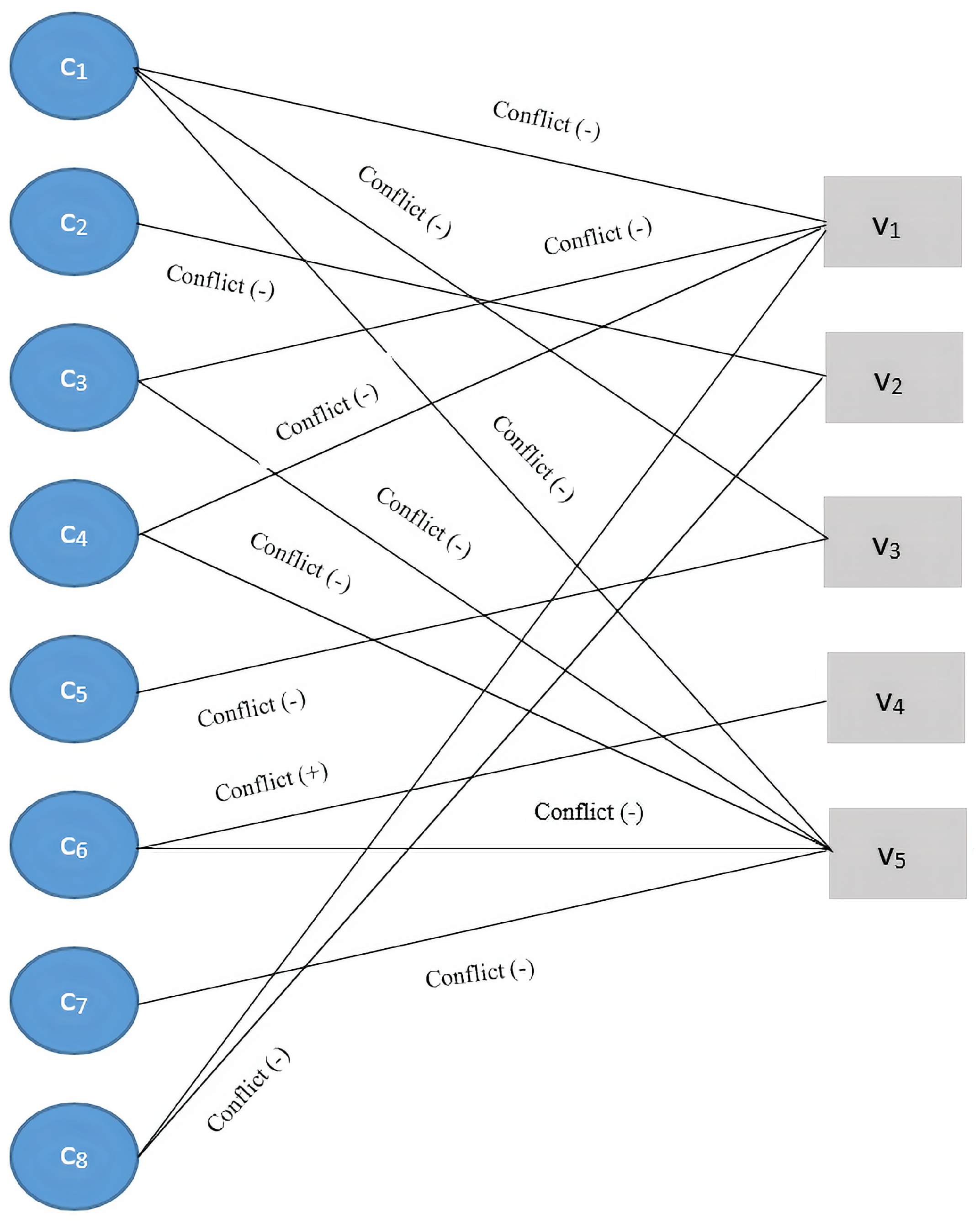
Figure 3 presents the flow graph of Table 19 and the conflict situation in the given Table 20 through visual representation. The given flow graph in the figure illustrates each mapping between the context and video on the basis of some conflict status (+), (-), and (0).

The negative (-) sign represents the existence of a conflicting situation, the positive (+) sign indicates that there is no conflicting situation, and 0 represents that a corresponding video has not been watched in the current context.

Step 2 (Calculating Lower Approximation):

In this phase, we will compute lower approximation on the soft set which has been demonstrated in a previous step. This set will contain only those objects that surely belong to the set X. Lower approximation will be computed by assuming value of X as follows:

$${\underline{S}}_P\left(X\right)=\{uϵU:\exists eϵE,[uϵF\left(e\right)\subseteq X]\}.$$

Let us consider our X = {$v_1$, $v_3$} which is one of the subsets from the P(V) where V represents the videos, then the lower approximation will be:

$${\underline{S}}_P\left(X\right)=\{\mathit{F}({\mathit{c}}_{\mathit{i}},{\mathit{v}}_1),\mathit{F}({\mathit{c}}_{\mathit{i}},{\mathit{v}}_3)\}\to \mathit{F}\left(c_1\right).$$

Similarly, if X = {$v_1$, $v_2$}, then the lower approximation set will become:

$${\underline{S}}_P\left(X\right)=\{\mathit{F}({\mathit{c}}_{\mathit{i}},{\mathit{v}}_1),\mathit{F}({\mathit{c}}_{\mathit{i}},{\mathit{v}}_2)\}\to \mathit{F}\left(c_8\right),$$

where v represents a video and c${}_i$ represents any context scenario in which video v has been watched. To better illustrate this concept, consider the scenario given in Table 19. From the illustrated example, it is demonstrated that a given combination of videos which we have taken in set X is efficient to recommend in context $c_1$ because videos watched in $c_1$ has maximum matching with a given set X. Hence, we can compute a relevant context scenario for each subset of video combination. As our lower approximation set ${\underline{S}}_P\left(X\right)$ is not empty, hence, we will perform upper approximation ${\overline{S}}_P\left(X\right)$ on the given soft sets.

Step 3 (Calculating Upper Approximation):

In this phase, we will compute upper approximation on the soft set which has been created in step 1. This set will contain those objects that possibly belong to the set X. Upper approximation will be computed by assuming value of X as follows:

$${\overline{S}}_P\left(X\right)=\{uϵU:\exists eϵE,[uϵF\left(e\right),F\left(e\right)\cap X\ne \varnothing ]\}.$$

If our X = {$v_1$, $v_3$}, then upper approximation will be:

Let us consider our X = {$v_1$, $v_3$}, which is one of the subsets from the P(V), where V represents the videos, then the upper approximation will be: ${\overline{S}}_P\left(X\right)$={F(c${}_i$,v${}_1$), F(c${}_i$,v${}_3$)}→F($c_1$), F($c_3$), F($c_4$), F($c_5$), F($c_8$).

As can be seen from the above approximations, it indicates that, with a given combination of videos in set X, possible contextual scenarios can be $c_1$, $c_3$, $c_4$, $c_5$ and $c_8$.

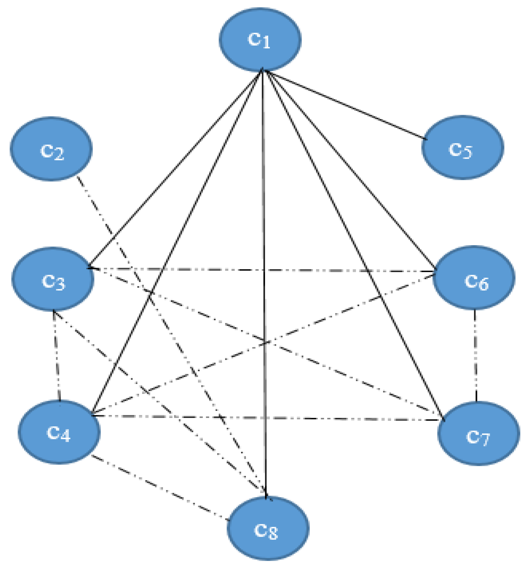
Step 4 (Degree of Dependency using Positive Region):

This phase is performed immediately after the calculation of lower ${\underline{S}}_P\left(X\right)$ and upper approximation ${\overline{S}}_P\left(X\right)$ to access the degree of dependency between the attributes using positive region POS${}_A$(X). Figure 4 presents the degree of dependency between each of the contextual scenarios obtained from Table 20.

As can be seen from Figure 4, each branch represents the link of a contextual scenario with other context scenarios. It gives a clear indication of dependency between different context attributes. For clarity and simplicity, solid lines denote a high degree of dependency, and the dotted lines represent low dependency between the attributes.

In the given circumstance, a contextual scenario c${}_i$ is revoked of an attribute v${}_i$. Suppose our X = {$v_1$, $v_3$} which is one of the subsets from the P(V), where V represents the videos, the degree of dependency of contextual scenario for this subset can be computed using Equation (9). For this particular scenario, POS${}_A$(X) will be c${}_1$, and |O| will be the whole set of videos V = {$v_1$,$v_2$,$v_3$,$v_4$,$v_5$}. Likewise, the calculations using Equation (9) will be incorporated in Equation (11) for computing degree of dependency ${\gamma }_a$, where a$ϵ$ A. For the sake of simplicity and clarity, each calculation is given below:

$${\mathrm{POS}}_A\left(\mathrm{X}\right)={\underline{\mathrm{S}}}_P\left(X\right)\Rightarrow {\mathit{c}}_1.$$

Respectively, ${\gamma }_A$ computing dependency of X on A as:

$${\gamma }_A=\frac{c_1}{\{v_1,v_1,v_2,v_4,v_5\}}.$$

Finally, degree of dependency ${\gamma }_a$ will be computed as given below:

$${\gamma }_a={\gamma }_A-{\gamma }_{A-{\sum }_{i=1}^n{c}_i};n=5.$$

After the association of degree of dependency between the c${}_1$ and all remaining contextual scenarios from the set A, we can now compute the relevant contexts through this dependency level.

Step 5 (Weighting Process):

We will use lower approximation while generating decision rules for exploiting relevant context. In our case, it can be seen that the relevant context for the given subset X in Step 2 is $c_1$. However, other videos can be achieved by applying the same mechanism on different subsets of videos.

The key intuition behind using a soft-rough set process, rather than traditional approaches, is that high precision is achieved by making real estimates through identifying imprecise data. For the weighting process, we assume that those contextual attributes that are less dependent on other contextual features are more valuable in making predictions. The weighting factor w will consider the weight as the real values in the range of [0,1]. These weights for each of the contextual attributes manipulate the influence of those factors by controlling their overall contribution during recommendation.

In the given circumstance, the degree of dependency can be computed from step 4 by following the methodology defined in that section. Likewise, Figure 4 illustrates the degree of dependency between different contextual scenarios. As interesting as it may appear, each contextual scenario is a combination of different contextual attributes. Hence, the degree of dependency of each contextual scenario actually depicts the level of dependency of particular contextual scenarios with other contextual attributes. We had divided dependency into three categories: completely dependent, partially dependent, and least dependent for the purpose of assigning weights. Table 20 reflects the degree of dependency for each contextual attribute as demonstrated below:

c${}_1$ = Highest Dependency ⇒ Child, Day, Weekday,

c${}_2$ = Least Dependency ⇒ Child, Day, Weekend,

c${}_3$ = Partial Dependency ⇒ Child, Night, Weekday,

c${}_4$ = Partial Dependency ⇒ Child, Night, Weekend,

c${}_5$ = Least Dependency ⇒ Adult, Day, Weekday,

c${}_6$ = Partial Dependency ⇒ Adult, Day, Weekend,

c${}_7$ = Partial Dependency ⇒ Adult, Night, Weekday,

c${}_8$ = Partial Dependency ⇒ Adult, Night, Weekend.

Likewise, degree of dependency for each contextual attribute from the above illustrative equation can be computed in a way that highest dependency weight is 0.2, the weight for partial dependency is 0.3, and, lastly, the weight for least dependency is 0.5 as demonstrated below:

$$Weights=\left\{\begin{array}{c}Age=\left\{\begin{array}{c}Child\Rightarrow 1.3,\\ Adult\Rightarrow 1.4,\end{array}\right.\\ Time=\left\{\begin{array}{c}Day\Rightarrow 1.5,\\ Night\Rightarrow 1.2,\end{array}\right.\\ DayType=\left\{\begin{array}{c}Weekday\Rightarrow 1.3,\\ Weekend\Rightarrow 1.4.\end{array}\right.\end{array}\right.$$

For each contextual attribute, the total weights are calculated through the sum of individual weight associated due to their occurrence in each of the dependency level. As an example, Child occurs in four different contextual scenarios, with different dependency levels. Thus, by summing these up, the dependency level will generate the total weight of the Child attributes.

Step 6 (Selection of Relevant Contextual Attribute):

The above-computed weights are being used for relevant context prediction for a given set of videos. A new minimum contextual set is chosen for the recommendation process. Supposing that a combination of videos is given as X = {$v_1$, $v_3$}, then the most suitable contextual scenario in which this combination of videos has to be recommend will be F($c_1$), as F($c_1$) is the combination of three contextual attributes {Child, Day, Weekday}. Thus, the most influential contextual factors from these three attributes will be the one with maximum weight among them. Hence, for the given circumstance, the most influential context will be Day, which actually represents the Time attribute. Respectively, we can ignore other contextual attributes by selecting only the minimal part from the set of contextual attributes.

It had been indicated from the literature that using irrelevant contextual features in recommender algorithms may agitate contextual sparsity. Therefore, the selection of contextual sets with minimal contextual factors can alleviate the contextual sparsity. After the detection of the relevant contextual set containing minimal but influential contextual factors, the recommendation process will start. One of the most popular approaches that is the most successful while predicting recommendations for the videos in CAVRS is collaborative filtering (CF). According to this approach, a comparison will be performed between the ratings of the current user and the rating of other users with similar history.

However, to confirm the genuineness of the results from the given illustrative example, we extensively analyzed the given scenario for the example, and our findings revealed that the conflicting situation reduces when a minimal set of contextual factors are used as contextual scenarios. We can, therefore, recommend the videos to the users on the basis of contextual scenarios containing minimal and highly weighted contextual factors.

6. Experiments

In this section, we illustrated the experiments for calculating the accuracy of our proposed approach. This section is organized as follows. Firstly, we describe the dataset required to report the results of our experiments, followed by demonstrating a methodology to fill missing values in the given dataset. Subsequently, we demonstrate the experiments we conducted to calculate the accuracy of our proposed scheme by evaluation setup, namely, the evaluation protocol, evaluation measure, and methods compared. Lastly, we report the results of our experiments on the dataset of LDOS-CoMoDa [13].

6.1. Experimental Setup

6.1.1. Context-Rich Dataset

For the purpose of comparing our proposed scheme with traditional approaches for determining its accuracy and effectiveness, we required a contextually rich dataset. Mostly used datasets in several studies on CAVRS, unfortunately, contains only specific contextual factors that are drivable using timestamps [13]. Likewise, other attributes included in these datasets are general information of the user such as age, gender, etc., which remain constant for a particular user, and thus these attributes cannot be utilized for computing user–item interaction with a varying degree of contextual factors [21].

As our main focus is inspecting a context-rich dataset with different contextual attributes, we performed a literature survey for identifying context-rich datasets containing potential pieces of contextual information. Several studies [13,21,23] have suggested LDOS-CoMoDa as the most contextually-rich dataset. LDOS-CoMoDa contains different variables related to the user, among which are 12 contextual factors. We have selected these 12 factors as of our interest as defined in

Table 21. Contextual attributes with their catagorical values.

Contexts	Description
Time	Morning, Afternoon, Evening, Night
Daytype	Working day, Weekend, Holiday
Season	Spring, Summer, Autumn, Winter
Location	Home, Public place, Friend’s house
Weather	Sunny/clear, Rainy, Stormy, Snowy, Cloudy
Social	Alone, My partner, Friends, Colleagues, Parents, Public, My family
EndEmo	Sad, Happy, Scared, Surprised, Angry, Disgusted, Neutral
DominantEmo	Sad, Happy, Scared, Surprised, Angry, Disgusted, Neutral
Mood	Positive, Neutral, Negative
Physical	Healthy, Ill
Decision	User decided which movie to watch, User was given a movie
Interaction	First, interaction with a movie, n-th interaction with a movie

. Other variables are general user information (age, sex, city, country) and content (movie) metadata (director, movieCountry, movieLanguage, movieYear, genre1, genre2, genre3, actor1, actor2, actor3, budget). In terms of statistical values, however, all of the mentioned factors contain categorical attributes.

The data in LDOS-CoMoDa had been explicitly acquired from the user through a web-based platform [13]. The size of LDOS-CoMoDa subsequently provides sufficient information to analyze several contextual issues. However, it contains 4% of missing values due to various reasons, such as manual data entry procedures and incorrect measurements [23].

Missing attribute values are a common problem in knowledge discovery from data processes [44]. One of the major contribution of this paper is the filling of these missing values. We have used the rough set as a technique to predict the missing values in the dataset of LDOS-CoMoDa in this research. The accuracy of prediction is compared with kNN, the most common attribute value (MCV), and artificial neural network (ANN) methods.

RST based Missing Value Prediction: We had already defined the fundamentals of RST in Section 3.2. In this section, we will define the RST based technique for filling missing values in LDOS-CoMoDa.

We find from the literature [44,45] that the authors can predict the missing values only for decision attributes’ values. However, the RST based missing value prediction approach proposed by [46] claims that, using RST, we can predict missing values for any attributes (condition or decision attributes) and can predict all missing values. The RST based model [44] depends on the distance function to detect any missing attributes values. The distance function between complete information system table and incomplete information system table will be calculated for this purpose.

Definition 11.

Let X${}_{incomp}$, X${}_{comp}$ϵ U, where X${}_{incomp}$ is an incomplete decision table and X${}_{comp}$ represent a complete decision table, e${}_i$ϵ E the set of parameters, and N defines total number of parameters:

$$dis(X_{incomp},X_{comp})=\sqrt{\sum _{i=1}^N{[e_i\left(X_{incomp}\right)-e_i\left(X_{comp}\right)]}^2},$$

(27)

where e${}_i$(X${}_{incomp}$) is the value of attribute e with respect to the case X${}_{incomp}$.

The method will eliminate the attributes that have a small effect on the information system using the degree of dependency, which is a crucial aspect of RST. A complete description of this model is given in [45].

It has been indicated from the literature; no approach has been utilized for filling missing values in LDOS-CoMoDa. We compare the performance of RST based missing values prediction to the kNN and ANN based approaches, considering the correlation level between dataset entities. The lower the correlation level, the higher the accuracy; as in a real-world scenario, the explicit ratings from the user usually have minimum correlation [44]. Likewise, our proposed model assigns weights on the basis of minimum dependency. Hence, the dataset filled using RST contains a low correlation which reflects its accuracy. Figure 5 shows a comparison of these approaches.

6.1.2. Evaluation Protocol

Traditionally, recommender systems are evaluated using holdout methods [14]. According to the holdout method, a dataset is split into two parts, namely, a training set and a testing set. A recommended model is trained on the training set, and the effectiveness of that set is evaluated using the testing set through experiments [20]. However, these methods have their own limitations for synthesis datasets [21], mainly because, when we randomly rate data for training and testing, it ignores the original order of observations and loses the temporal dimensions.

In order to simulate a realistic contextually-aware video recommendation scenario in our evaluation, we select all 12 contextual attributes along with 4138 videos from our dataset of LDOS-CoMoDa. By having multiple such contextual attributes, we can assess the effectiveness of each recommendation through a training process. In particular, each contextual feature simulates a situation when a video recommendation has been generated.

Since the video recommendation requires an initial phase of training, we adopt the evaluation process proposed in [23], we firstly sort our dataset of LDOS-CoMoDa chronologically and then split it into the following subsets:

• Training Subset contains the first 20% of our dataset for training our model by including 828 videos and 367 unique contextual scenario created by the 12 contextual features.
• Testing Subset contains the next 30% of our dataset for validating the initialized model.
• Test and Train from learning This subset contains the next 50% of our dataset in which the test-then-learn procedure performed while iterating over the observations. Each observation will be used for evaluating the model by generating recommendations and then updating the model by learning.

6.1.3. Evaluation Measures

We make a comparison between basslines and proposed models based on the accuracy of prediction for relevant context selection. We used Rstudio version 3.5.2 (RStudio, Inc., Boston, MA, USA) for computing results from all approaches. We also execute all approaches for comparison on an Intel Core i7 CPUs processor (Santa Clara, CA, USA) with RAM of 16 GB and Windows 10 as the operating system (Microsoft, Redmond, WA, USA).

We use recall@N and DCG@N to measure the effectiveness of recommendation through our proposed model. The recall@n is used to calculate the ratio of accurately predicted ratings for the recommendation of videos to the total number of useful recommendations. We have applied precision as an evaluation metrics using Equation (28) for SRS-CaVRS:

$$Recall=\frac{AccuratePredictionsforRecommendation}{TotalUsefulRecommendation}.$$

(28)

Similarly, the DCG@n is used to measure the quality of the ranking predicted by the proposed algorithm at nth recommendations. The gain is collected from the highest point of the outcome rundown to the base, with the increase of each outcome limited at lower positions. It can be denoted as:

$$DC{G}_i=\sum _{j=1}^i\frac{re{l}_j}{lo{g}_2(j+1)},$$

(29)

where $re{l}_i$ represents the significance of the results at a given point j. Likewise, i denotes the ranking position.

These metrics consider the top recommendation in highly non-stationary contextual environments for the online setting when the given dataset is large [20]. We report our results for the Test and Train from learning subset.

6.1.4. Baselines Compared and Parameters

To assess the effectiveness of our proposed model, we compare it to several state-of-the-art methods that had been used for selecting a relevant context by alleviating contextual sparsity. In order to obtain the parameters that result in the best performance, we performed a grid search over the parameter space of the methods. We report the performance results with regard to those parameters, which leads to the best outcome. The baselines compared along with their selected parameters, are given below:

• SRS-CaVRS is the method we proposed, combining soft sets based representation of the conflicting situation in Boolean-valued information system and rough set based formal approximation on that soft set. For LDOS-CoMoDa, we set the number of contextual scenarios (U) (Equation (12)) = 367 and videos (V) (Equation (12)) = 828
• RST relies on formal approximation using the dependency level for reducing attributes. It replaces traditional methods with formal approximation using the boundary region. For LDOS-CoMoDa, we set the number of contextual scenarios (U) = 367 and videos (V) = 800
• DWR relies on using different weights for exploiting relevant contextual information during the development of CARS. For LDOS-CoMoDa, we set the number of contextual scenarios (U) = 367 and videos (V) = 750
• DCR relies on using different subsets of contextual attributes for utilizing different components of recommender algorithms. For LDOS-CoMoDa, we set the number of contextual scenarios (U) = 367 and videos (V) = 750
• t-Test is used for the detection of influential contextual features in a given dataset. For LDOS-CoMoDa, we set the number of contextual scenarios (U) = 367 and videos (V) = 700.

The parameters that are used for all baseline models were defined by a grid search on the validation sets.

6.2. Results and Discussion

In this phase, we will assess the overall performance of SRS-CaVRS by explicitly answering each of the following formulated research questions:

Q1. What is the overall effectiveness of SRS-CaVRS to alleviate contextual sparsity in CAVRS?

Q2. Which contextual factors are identified as an influencer in the recommendation process?

In the forthcoming section, we attempted to address the above formulated research question to assess the performance of our proposed scheme.

In particular, Figure 6 and Figure 7 show the recall@n and DCG@n performance of SRS-CaVRS in comparison to the baselines, which merge these approaches for training to rank videos. Our proposed model outperforms all individual recommendations. Likewise, the results of our proposed model on LDOS-CoMoDa for the test and train subset is given in

Table 22. Results for LDOS-CoMoDa on the Test and Train subset. Our proposed model SRS-CaVRS outperforms in both of the evaluation criteria. These results are in terms of Recall@n and DCG@n (bold-face indicates significant improvements over all the baselines RST and DWR).

Task	Algorithms	LDOS-CoMoDa
		Recall@n				DCG@n
		n = 5	n = 10	n = 50	n = 100	n = 5	n = 10	n = 50	n = 100
Alleviating Contextual Sparsity	RST ${}^a$	+10.58%(±0.07)	+9.38%(±0.07)	+7.03%(±0.06)	+5.93%(±0.05)	+10.58%(±0.07)	+9.38%(±0.07)	+7.03%(±0.06)	+5.93%(±0.05)
	DWR ${}^c$	+7.95%(±0.05)	+6.77%(±0.05)	+5.89%(±0.05)	+4.99%(±0.04)	+7.95%(±0.05)	+6.77%(±0.05)	+5.89%(±0.05)	+4.99%(±0.04)
	DCR ${}^b$	+6.90%(±0.05)	+5.03%(±0.05)	+4.67%(±0.05)	+3.81%(±0.04)	+6.90%(±0.05)	+5.03%(±0.05)	+4.67%(±0.05)	+3.81%(±0.04)
	t-Test	+3.64%(±0.04)	+2.93%(±0.04)	+1.87%(±0.04)	+0.90%(±0.04)	+3.64%(±0.04)	+2.93%(±0.04)	+1.87%(±0.04)	+0.90%(±0.04)
	SRS-CaVRS${}^d$	+15.58%(±0.09)	+14.89%(±0.09)	+14.67%(±0.09)	+13.74%(±0.09)	+15.58%(±0.09)	+14.89%(±0.09)	+14.67%(±0.09)	+13.74%(±0.09)

${}^a$ RST: Rough Set Theory; ${}^b$ DCR: Differential Context Relaxation; ${}^c$ DWR: Differential Weightage Relaxation; ${}^d$ SRS-CaVRS: (Soft-Rough set based Context-aware video recommender system).

.

6.2.1. SRS-CaVRS Effectivness

As an attempt to address Q1, we computed the performance of SRS-CaVRS by comparing it with four baselines. Figure 6 demonstrates comparison results through Recall@n for video recommendation by LDOS-CoMoDa. The idea behind evaluation is the performance of each approach in terms of selecting relevant contextual attributes. It has been observed that SRS-CaVRS consistently outperforms all baselines. Indeed, SRS-CaVRS improves upon the strongest baseline RST based CARS. Moreover, we observe that the t-test shows a higher level of contextual sparsity in all values for n in both evaluation metrics. Since DWR has a comparatively better performance, this indicates that the weighting method is a suitable mechanism for selecting a relevant contextual scenario with the least contextual sparsity. Indeed, contextual sparsity can be handled through weighted features by formal approximation.

The experimental results show that the prediction of the scores using a minimal set of contextual attributes through soft-rough set can produce better results. Our proposed model has resulted in a 7% increase in the accuracy of the recommendation process as compared to the traditional models. Figure 6 shows the results of the comparison of baselines with the proposed model on taking the top n recommendations that had been extracted from each of the models. Through this observation, the extracted scores from the proposed model had been compared with the baseline approaches. The idea behind this comparison was that the ratings for the ranking process that had been collected through the algorithms will be compared with the ratings available in the dataset to check if the proposed model has returned top rated scored videos using a minimal set of users’ contextual attributes.

Moreover, Figure 7 demonstrates comparison results through nDCG for video recommendations by LDOS-CoMoDa. The idea behind evaluation is the gain of each approach in terms of selecting relevant contextual attributes. It has been observed that SRS-CaVRS consistently outperforms all baselines. Indeed, SRS-CaVRS improves upon the strongest baseline RST based CARS. Moreover, it observes that the t-test shows a lower level of gain in all values for n cases in nDCG evaluation metrics. Since DWR has a comparatively better performance, which indicates that the weighting method is a suitable mechanism for selecting a relevant contextual scenario with the least contextual sparsity. Indeed, contextual sparsity can be handled through weighted features by formal approximation.

6.2.2. Effective Contextual Features

To address Q2, we further analyze the performance of SRS-CaVRS from the aspect of selecting relevant contextual features. Applying SRS-CaVRS in LDOS-CoMoDa demonstrates that users’ moods are the most influential contexts among all available contextual features. Therefore, the weights of each contextual attribute depend on the preference of the user. The user can fine-tune the values on the basis of which weights can be assigned. It can be understood in a way that the contextual attributes have a conflicting situation if the same videos are watched in multiple contexts. Hence, the mood of the user is also kept under consideration each time. Therefore, on the basis of change in the preferences of the user, the overall conflicting situation between contextual attributes will also change. Subsequently, it will affect the weight assigning process.

In particular, Figure 6 and Figure 7 show the recall@n and DCG@n performance of SRS-CaVRS in comparison to the baselines, which merge these approaches for training to rank videos. Our proposed model outperforms all individual recommendations. The selection of most the relevant contextual scenario has been done through the weights assigning technique through soft-rough sets.

6.2.3. Threats to Validity

For a comprehensive analysis of the results acquired from our experimental setup, limitations in our study must be considered. The main threat to our experiment is the validation of our proposed scheme using only a single dataset. The results from the proposed scheme are validated by using LDOS-CoMoDa dataset by showing the accuracy of the proposed algorithm in handling contextual sparsity by exploiting relevant contextual factors. However, LDOS-CoMoDa contains missing values up to 4%, which are a common problem in knowledge discovery from data processes. We have used Rough sets as a technique to predict the missing values in the dataset of LDOS-CoMoDa in this research. However, different attribute reduction approaches can also be used to fill these missing values in an efficacious way. Similarly, it is not possible to restrict all the contextual attributes of the users to categorical values. Factors like location or social given in our dataset are usually non-categorical. However, in this study, we have used only the standard values of contextual attributes given in the dataset of LDOS-CoMoDa. These categorical values have been provided as part of the dataset LDOS-CoMoDa by the creators. The main focus of this study was the evaluation of the proposed scheme on a contextually rich dataset. The dataset of LDOS-CoMoDa contains 12 contextual factors with categorical values. Hence, we have only focused on these specific values by considering them categorical in this case. However, standard soft sets seem not to be suitable to handle non-categorical values. Hence, an extended version N-Soft sets can be used to tackle this limitation [47]. Nevertheless, there are no N-soft rough set models in the literature, and the use of N-Soft sets for handling non-categorical values of contextual attributes will be our future task.

7. Conclusions and Future Directions

In this article, we attempted to address the issue of contextual sparsity in CAVRS through a soft-rough set based model for assigning weights to reduce contextual attributes for selecting a relevant context. The proposed approach, namely SRS-CaVRS, is developed to cope with alleviating contextual sparsity in an efficacious way. It merges the crucial aspect of a soft set in which a conflicting situation is represented as a Boolean-valued information system, and the formal approximation technique of RST for attributes’ reduction. To the best of the author’s knowledge, this study provides a first attempt to leverage a soft set, hybridized with rough sets, for handling the problem of contextual sparsity in CAVRS. Since our proposed approach required some training, hence, SRS-CaVRS is effective in terms of computation performance.

In a thorough evaluation of the proposed approach on a contextually rich dataset of LDOS-CoMoDa, we proved the effectiveness of the proposed scheme SRS-CaVRS. Since, unlike other classical approaches, we are able to leverage the large sample of data with a conflict situation, SRS-CaVRS outperforms all the classical models, in addition to the recent approaches such as RST based CARS, DWR, and DCR. Our results depict many interesting conclusions, such as:

• The representation of the conflicting situation in a Boolean-valued information system can lead to highly accurate recommendations by alleviating contextual sparsity.
• The weight assigning process through formal approximation results in influential contexts that are far more relevant than the contexts obtained through state-of-the-art models.

In particular, it has been shown that SRS-CaVRS, a hybridization of a soft set with RST in CAVRS, has outstanding performance, but the idea of combining a soft set with a decision-making technique (such as RST) can be extended to other domain areas as well. Future directions may consider new areas for trying out further hybridization techniques such as Soft set based AHP and Soft set based fuzzy set theory in CAVRS, and will investigate how adaptive hybridized soft sets can be extended to alleviate contextual sparsity from CAVRS. Likewise, to handle contextual factors with non-categorical values, standard soft sets seem to not be suitable to handle non-categorical values. Hence, an extended version N-Soft sets can be used to tackle this limitation. Nevertheless, there are no N-soft rough set models in the literature, and the use of N-Soft sets for handling non-categorical values of contextual attributes will be our future task.

References

1. Adomavicius, G.; Tuzhilin, A. Context-aware recommender systems. In Recommender Systems Handbook; Springer: Boston, MA, USA, 2011; pp. 217–253. [Google Scholar]
2. Adomavicius, G.; Tuzhilin, A.; Berkovsky, S.; De Luca, E.W.; Said, A. Context-aware recommender systems: Research workshop and movie recommendation challenge. In Proceedings of the RecSys 2010, Barcelona, Spain, 26–30 September 2010; pp. 26–30. [Google Scholar]
3. Panniello, U.; Tuzhilin, A.; Gorgoglione, M. Comparing context-aware recommender systems in terms of accuracy and diversity. User Model. User-Adapt. Interact. 2014, 24, 35–65. [Google Scholar] [CrossRef]
4. Liu, X.; Aberer, K. SoCo: A social network aided context-aware recommender system. In Proceedings of the 22nd International Conference on World Wide Web, Rio de Janeiro, Brazil, 13–17 May 2013; pp. 781–802. [Google Scholar]
5. Knijnenburg, B.P.; Kobsa, A. Making decisions about privacy: Information disclosure in context-aware recommender systems. ACM Trans. Interact. Intell. Syst. 2013, 3, 20. [Google Scholar] [CrossRef]
6. Champiri, Z.D.; Shahamiri, S.R.; Salim, S.S.B. A systematic review of scholar context-aware recommender systems. Expert Syst. Appl. 2015, 42, 1743–1758. [Google Scholar] [CrossRef]
7. Abbas, M.; Riaz, M.U.; Rauf, A.; Khan, M.T.; Khalid, S. Context-aware Youtube recommender system. In Proceedings of the IEEE International Conference on Information and Communication Technologies (ICICT), Karachi, Pakistan, 30–31 December 2017; pp. 161–164. [Google Scholar]
8. Baltrunas, L.; Ludwig, B.; Ricci, F. Matrix factorization techniques for context aware recommendation. In Proceedings of the Fifth ACM Conference on Recommender Systems, Chicago, IL, USA, 23–27 October 2011; pp. 301–304. [Google Scholar]
9. Abbas, A.; Zhang, L.; Khan, S.U. A survey on context-aware recommender systems based on computational intelligence techniques. Computing 2015, 97, 667–690. [Google Scholar] [CrossRef]
10. Abbas, S.M.; Riaz, M.U.; Rauf, A.; Khan, M.T.; Khalid, S. Improved Context-aware YouTube Recommender System with User Feedback Analysis. Bahria Univ. J. Inf. Commun. Technol. 2017, 10, 1–8. [Google Scholar]
11. Peña, F.J. Unsupervised Context-Driven Recommendations Based On User Reviews. In Proceedings of the Eleventh ACM Conference on Recommender Systems, Como, Italy, 27–31 August 2017; pp. 426–430. [Google Scholar]
12. Baltrunas, L.; Ludwig, B.; Peer, S.; Ricci, F. Context relevance assessment and exploitation in mobile recommender systems. Pers. Ubiquitous Comput. 2012, 16, 507–526. [Google Scholar] [CrossRef]
13. Odić, A.; Tkalćić, M.; Tasić, J.F.; Kośir, A. Relevant context in a movie recommender system: Users’ opinion vs. statistical detection. In Proceedings of the CARS-2012, Dublin, Ireland, 9 September 2012. [Google Scholar]
14. Adomavicius, G.; Sankaranarayanan, R.; Sen, S.; Tuzhilin, A. Incorporating contextual information in recommender systems using a multidimensional approach. ACM Trans. Inf. Syst. 2005, 23, 103–145. [Google Scholar] [CrossRef] [Green Version]
15. Huang, Z.; Lu, X.; Duan, H. Context-aware recommendation using rough set model and collaborative filtering. Artif. Intell. Rev. 2011, 35, 85–99. [Google Scholar] [CrossRef]
16. He, M.; Ren, W. Attribute reduction with rough set in context-aware collaborative filtering. Chin. J. Electron. 2017, 26, 973–980. [Google Scholar] [CrossRef]
17. Liu, L.; Lecue, F.; Mehandjiev, N.; Xu, L. Using context similarity for service recommendation. In Proceedings of the IEEE Fourth International Conference on Semantic Computing, Pittsburgh, PA, USA, 22–24 September 2010; pp. 277–284. [Google Scholar]
18. Haruna, K.; Ismail, M.A.; Suyanto, M.; Gabralla, L.A.; Bichi, A.B.; Danjuma, S.; Herawan, T. A Soft Set Approach for Handling Conflict Situation on Movie Selection. IEEE Access. 2019. [Google Scholar] [CrossRef]
19. Huang, H. Context-aware location recommendation using geotagged photos in social media. ISPRS Int. J. Geo-Inf. 2016, 5, 195. [Google Scholar] [CrossRef]
20. Zheng, Y.; Burke, R.; Mobasher, B. Recommendation with differential context weighting. In Proceedings of the International Conference on User Modeling, Adaptation, and Personalization, Rome, Italy, 10–14 June 2013; pp. 152–164. [Google Scholar]
21. Dixit, V.S.; Jain, P. Recommendations with Sparsity Based Weighted Context Framework. In Proceedings of the International Conference on Computational Science and Its Applications, Melbourne, VIC, Australia, 2–5 May 2018; pp. 289–305. [Google Scholar]
22. Zheng, Y. A revisit to the identification of contexts in recommender systems. In Proceedings of the 20th International Conference on Intelligent User Interfaces Companion, Atlanta, GA, USA, 29 March–1 April 2015; pp. 133–136. [Google Scholar]
23. Dixit, V.S.; Jain, P. Weighted Percentile-Based Context-Aware Recommender System. In Applications of Artificial Intelligence Techniques in Engineering; Springer: Berlin/Heidelberg, Germany, 2019; pp. 377–388. [Google Scholar]
24. Zheng, Y.; Burke, R.; Mobasher, B. Differential context modeling in collaborative filtering. In Proceedings of the School of Computing Research Symposium, Chicago, IL, USA, 31 May 2013. [Google Scholar]
25. Zheng, Y.; Burke, R.; Mobasher, B. Differential context relaxation for context-aware travel recommendation. In Proceedings of the International Conference on Electronic Commerce and Web Technologies, Vienna, Austria, 4–5 September 2012; pp. 88–99. [Google Scholar]
26. Zheng, Y.; Burke, R.; Mobasher, B. Optimal feature selection for context-aware recommendation using differential relaxation. In Proceedings of the Sixth ACM Conference on Recommender Systems (RecSys’12), Dublin, Ireland, 9 September 2012. [Google Scholar]
27. Li, H.; Zhang, W.; Xu, P.; Wang, H. Rough set attribute reduction in decision systems. In Proceedings of the International Conference on Rough Sets and Knowledge Technology, Chongqing, China, 24–26 July 2006; pp. 135–140. [Google Scholar]
28. Wang, C.; Huang, Y.; Shao, M.; Fan, X. Fuzzy rough set-based attribute reduction using distance measures. Knowl. -Based Syst. 2019, 164, 205–212. [Google Scholar] [CrossRef]
29. Wang, C.; Shi, Y.; Fan, X.; Shao, M. Attribute reduction based on k-nearest neighborhood rough sets. Int. J. Approx. Reason. 2019, 106, 18–31. [Google Scholar] [CrossRef]
30. Chen, H.; Li, T.; Cai, Y.; Luo, C.; Fujita, H. Parallel attribute reduction in dominance-based neighborhood rough set. Inf. Sci. 2016, 373, 351–368. [Google Scholar] [CrossRef] [Green Version]
31. Pawlak, Z. Rough sets. Int. J. Comput. Inf. Sci. 1982, 11, 341–356. [Google Scholar] [CrossRef]
32. Ali, M.A. A note on soft sets, rough soft sets and fuzzy soft sets. Appl. Soft Comput. 2011, 11, 3329–3332. [Google Scholar]
33. Alam, K.A.; Ahmad, R. A hybrid fuzzy multi-criteria decision model for cloud service selection and importance degree of component services in service compositions. In Proceedings of the 12th International FLINS Conference, Roubaix, France, 24–26 August 2016. [Google Scholar]
34. Zhan, J.; Zhang, X.; Yao, Y. Covering based multigranulation fuzzy rough sets and corresponding applications. Artif. Intell. Rev. 2019, 1–34. [Google Scholar] [CrossRef]
35. Khan, M.T.; Azam, N.; Khalid, S.; Yao, J. A three-way approach for learning rules in automatic knowledge-based topic models. Int. J. Approx. Reason. 2017, 82, 210–226. [Google Scholar] [CrossRef]
36. Nauman, M.; Azam, N.; Yao, J. A three-way decision-making approach to malware analysis using probabilistic rough sets. Inf. Sci. 2013, 374, 193–209. [Google Scholar] [CrossRef]
37. Zhan, J.; Liu, Q.; Herawan, T. A novel soft rough set: Soft rough hemirings and corresponding multicriteria group decision-making. Appl. Soft Comput. 2017, 54, 393–402. [Google Scholar] [CrossRef]
38. Malik, N.; Shabir, M. Rough fuzzy bipolar soft sets and application in decision-making problems. Soft Comput. 2019, 23, 1603–1614. [Google Scholar] [CrossRef]
39. Sun, B.; Ma, W. Soft fuzzy rough sets and its application in decision-making. Artif. Intell. Rev. 2014, 41, 67–80. [Google Scholar] [CrossRef]
40. Herawan, T.; Deris, M.M. A soft set approach for association rules mining. Knowl.-Based Syst. 2011, 24, 186–195. [Google Scholar] [CrossRef]
41. Wang, C.; Qi, Y.; Shao, M.; Hu, Q.; Chen, D.; Qian, Y.; Lin, Y. A fitting model for feature selection with fuzzy rough sets. IEEE Trans. Fuzzy Syst. 2017, 25, 741–753. [Google Scholar] [CrossRef]
42. Feng, F.; Liu, X.; Leoreanu-Fotea, V.; Jun, Y.B. Soft sets and soft rough sets. Inf. Sci. 2011, 181, 1125–1137. [Google Scholar] [CrossRef]
43. Liu, Y.; Qin, K.; Martínez, L. Improving decision-making approaches based on fuzzy soft sets and rough soft sets. Appl. Soft Comput. 2018, 65, 320–332. [Google Scholar] [CrossRef]
44. Alam, K.A.; Ahmed, R.; Butt, F.S.; Kim, S.G.; Ko, K.M. An uncertainty-aware integrated fuzzy AHP-WASPAS model to evaluate public cloud computing services. Procedia Comput. Sci. 2018, 130, 504–509. [Google Scholar] [CrossRef]
45. Grzymala-Busse, J.W. A rough set approach to incomplete data. In Proceedings of the International Conference on Rough Sets and Knowledge Technology, Tianjin, China, 20–23 November 2015; pp. 3–14. [Google Scholar]
46. Çekik, R.; Telçeken, S. New Method Based on Rough Set for Filling Missing Value. In Recent Developments and the New Direction in Soft-Computing Foundations and Applications; Springer: Cham, Switzerland, 2018; pp. 41–48. [Google Scholar]
47. Fatimah, F.; Rosadi, D.; Hakim, R.F.; Alcantud, J.C.R. N-soft sets and their decision-making algorithms. Soft Comput. 2018, 22, 3829–3842. [Google Scholar] [CrossRef]
Figure 1. Incorporation of contextual information in the recommendation process. (a) Pre-filterining approch; (b) Post-filterining approch; (c) Contextual modeling
Mathematics 07 00740 g001
Figure 2. Architecture of the proposed scheme.
Mathematics 07 00740 g002
Figure 3. Conflict in given contextual attributes.
Mathematics 07 00740 g003
Figure 4. Conflict representation through soft sets.
Mathematics 07 00740 g004
Figure 5. Performance evaluation of RST and other approaches for the task of missing values filling with minimum correlation between the existing entities and filled entities of LDOS-CoMoDa dataset.
Mathematics 07 00740 g005
Figure 6. Results of proposed scheme SRS-CaVRS by using dataset of LDOS-CoMoDa. (a) results for Recall@5; (b) results for Recall@10; (c) results for Recall@50; (d) results for Recall@100.
Mathematics 07 00740 g006
Figure 7. Results of proposed scheme SRS-CaVRS by using dataset of LDOS-CoMoDa. (a) Results for DCG@n = 5; (b) Results for DCG@n = 10; (c) Results for DCG@n = 50; (d) Results for DCG@n = 100.
Mathematics 07 00740 g007