Modeling and Control of IPMC Actuators Based on LSSVM-NARX Paradigm

Abstract

Ionic polymer-metal composites are electrically driven intelligent composites that are readily exposed to bending deformations in the presence of external electric fields. Owing to their advantages, ionicpolymer-metal composites are promising candidates for actuators. However, ionicpolymer-metal composites exhibit strong nonlinear properties, especially hysteresis characteristics, resulting in severely reduced control accuracy. This study proposes an ionic polymer-metal composite platform and investigates its modeling and control. First, the hysteresis characteristics of the proposed Pt-electrode ionic polymer-metal composite are tested. Based on the hysteresis characteristics, ionic polymer-metal composites are modeled using the Prandtl-Ishlinskii model and the least squares support vector machine-nonlinear autoregressive model, respectively. Then, the ionic polymer-metal composite is driven by a random sinusoidal voltage, and the LSSVM-NARX model is established on the basis of the displacement data obtained. In addition, an artificial bee colony algorithm is proposed for accuracy optimization of the model parameters. Finally, an inverse controller based on the least squares support vector machine-nonlinear autoregressive model is proposed to compensate the hysteresis characteristics of the ionic polymer-metal composite. A hybrid PID feedback controller is developed by combining the inverse controller with PID feedback control, followed by simulation and testing of its actual position control on the ionic polymer-metal composite platform. The results show that the hybrid PID feedback control system can effectively eliminate the effects of the hysteresis characteristics on ionic polymer-metal composite control.

1. Introduction

Intelligent materials are among the most rapidly developing technologies globally [1]. In particular, intelligent polymer materials have attracted considerable attention owing to their light weight, large deformation, good biocompatibility, long service life, low cost, and reasonable mouldability. Such intelligent materials exhibit various responses (e.g., volume expansion, shape reconstruction, and color change) to external stimulations. Among intelligent polymer materials, electroactive polymers (EAPs) are novel flexible functional materials that undergo significant size variations under external electric fields, and they regain their original size upon removal of the external electric fields [2,3,4,5,6,7,8]. According to the actuation mechanism, EAPs can be categorized as ionic EAPs and electric-field EAPs. Ionic polymer-metal composites (IPMCs) are ionic EAPs that have been widely employed as actuators in bionics, biomedicine, and microelectronics, owing to their low actuating voltage (1–5 V), rapid response, large actuating displacement, good mouldability, and excellent flexibility [9,10,11,12,13,14,15,16].

In general, the ionicex change film of IPMCs contains moisture, and the water molecules combine with free hydrophilic cations to generate hydrated cations, which tend to migrate under electric fields. This phenomenon is the main contributor to the electric actuating function of IPMCs. Besides the matrix film, IPMCs contain upper and lower electrodes, which are typically noble metals such as Pt, Pd, Au, or Ag. Figure 1 shows the structure of the IPMC actuator.

Upon application of DC voltage, the IPMC actuator film immediately bends toward the anode, and then gradually toward the cathode during relaxation deformation [17]. The physical mechanism is as follows. Upon application of DC voltage, an electric field is developed between the electrodes and free cations in the matrix film combine with water molecules and migrate to the cathode, resulting in aggregation of water molecules near the cathode followed by swelling. Consequently, the actuator film bends toward the anode.

Nevertheless, as with other intelligent materials, IPMC control is limited by intrinsic nonlinear properties such as hysteresis and creep. Therefore, reducing the nonlinearity of IPMCs to minimize its adverse effects on IPMC control has been a research hotspot. The following subsections discuss the hysteresis characteristics of IPMCs through modeling and control.

1.1. Modeling

The study of IPMC modeling can be divided into two stages. In the first stage, studies of the electro chemical characteristics of IPMCs revealed their hysteresis characteristics and a circuit model reflecting their nonlinearity was established [18,19]. The hysteresis characteristics of IPMCs were shown to be affected by both the amplitude and the changing rate of stimulation voltage signals, and an improved circuit model was proposed [20]. However, the actuating mechanism of IPMCs was shown to be complicated. It involves not only charge movement but also other complicated changes such as structural reconstruction of molecular chains. In addition, the circuit model cannot explain the actuating characteristics of IPMCs, and its application range is limited. In the second stage, researchers were not confined by the actuating mechanism of IPMCs. A nonlinear model that combines an auto regressive neural network and a fuzzy algorithm was proposed. This model can effectively simulate the nonlinearity of the actuating displacement of IPMCs [21]. By combining an open-loop positioning strategy based on effective inversion with a dynamic Preisach operator, researchers proposed a cascade model to capture the hysteresis characteristics and dynamic properties of an IPMC actuator [22]. Furthermore, to investigate the hysteresis characteristics of IPMCs, a dynamic model of the IPMC actuator was realized by integrating a dynamic Preisach operator with a fuzzy NARX model and performing particle swarm optimization (PSO) [23]. Segmented modeling based on the finite element concept can effectively reflect the hysteresis characteristics of IPMCs [24]. Although the above-mentioned modeling approaches can reflect the nonlinearity of IPMCs, they do not consider the effects of environmental humidity on actuator performance. In other words, they do not consider actuator performance degradation due to dehydration after a long service time. As the migration of hydrated cations in IPMCs is the main cause of macroscopic IPMC deformation, previous studies have suggested that the IPMC actuating performance in humid conditions is superior to that in air. The hysteresis characteristics of an IPMC actuator under different temperatures and humidities were investigated and modeled using a non-autoregressive model based on the Laguerre multilayer perceptron network [25]. However, this model has high requirements in terms of the quality of the sample data, as it regards all data as feature data.

1.2. Control

Based on dynamic modeling studies, an IPMC actuator was positioned using the self-adaptive fuzzy algorithm for location control of an IPMC micro-pump [26]. The hysteresis characteristics of the IPMC actuator were analyzed using the discrete Prandtl-Ishlinskii model, the creep model of the IPMC actuator was obtained, and an inverse hysteresis model was developed by modifying the creep model of piezoelectric materials, followed by the development of a self-adaptive inverse control strategy for the displacement of the IPMC actuator [27]. In addition, a robust, discrete self-adaptive inverse control method and a discrete self-adaptive sliding mode control method were proposed [28,29,30]. In these control approaches, the IPMC actuator is regarded as a time-varying system, the dynamic model parameters of the actuator are set online by the control system, and the control parameters are adjusted accordingly. The control effect is significantly dependent on the efficiency and accuracy of the online setting, which is generally unreliable. Hence, time delay control (TDC), which exhibits good robustness in various control systems, was applied to IPMC actuators and the force control of a two-link manipulator driven by IPMC actuators [31,32]. The results indicated that, through this control approach, the IPMC actuator performance varies with the input sinusoidal actuating voltage and the effects of the hysteresis characteristics on the control accuracy are reduced. However, the applicability of this approach to systems driven by other signals needs to be verified. To overcome the intrinsic nonlinearity of IPMC actuators, external interferences, and other uncertain effects due to changes in the working environment, a nonsingular terminal sliding mode controller was developed [33]. Compared with conventional PID controllers, the nonsingular terminal sliding mode controller exhibits superior robustness. Considering changes in the water content of an IPMC actuator, a novel nonlinear self-adaptive observer was designed to determine the unknown potential and humidity in the matrix film, thus, the water content in an IPMC actuator operated for a long duration in air could be determined, and the accuracy of motion control could be improved [34]. Although these two methods focus on the effects of environment conditions on IPMC actuators, their control effects on the nonlinearity of an IPMC actuator, especially under significantly varying input actuating voltages, have not been clarified. Owing to the significant overshoot of open-loop responses of an IPMC actuator, the accuracy of closed-loop control is adversely affected. Therefore, a PSO-based IPMC optimized position control approach was proposed and proportional integration tuning parameters based on the conventional Ziegler-Nichols (ZN) method and PSO were compared with each other [35]. Thus, the advantages of PSO tuning over the conventional ZN method were demonstrated in the estimation of the optimized tuning parameters and the reduction of the effects of the hysteresis characteristics on the control accuracy of an IPMC actuator. However, this approach does not fundamentally solve the issue of low modeling accuracy. Instead, it reflects the advantages of PSO in parameter optimization.

In summary, current modeling approaches are not capable of effective and comprehensive simulation of the hysteresis characteristics of an IPMC actuator, resulting in high costs of the control systems. The support vector machine (SVM), based on statistical theory and structuralriskminimization principle, outperforms the artificial neural network in terms of global optimization and generalization capability [36] and it shows good performance in hysteresis modeling [37,38]. As an extension of SVM, the leastsquares support vector machine (LSSVM) overcomes the defect of slow trainingspeed in SVM by solving a linear equation set rather than aquadratic optimization problem [39]. Also, LSSVM has fewer parameters to be tuned [40], which means it can achieve accurate regression more easily. Therefore, LSSVM is an effective methodfor creating the hysteresis model and of IPMCs. However, LSSVM can only model one-to-one mapping, whereas the hysteresis nonlinearity is a multi-valued mapping. A practical way is to employ then on linear auto regressive exogenous (NARX) model, which represents an input-output recursive model [41]. The NARX model is widely employed for nonlinear system identification [42,43,44], where the current output is predicted by the current and previous inputs and previous outputs. The least squares support vector machine-nonlinear auto regressive exogenous integrates the two models of LSSVM and NARX effectively, and gives full play to the advantages of LSSVM in establishing a nonlinear model and NARX in processing a multi-valued mapping nonlinear system, which is particularly suitable for hysteresis modeling and control system design of IPMCs [45].Furthermore, owing to the actuating mechanism of IPMCs, an IPMC actuator exhibits better actuating performance and a longer service life in water than in air. Hence, IPMC actuators have wider and more promising applications in water. This study proposes the modeling of electrically driven tip displacement of an IPMC actuator in water using the LSSVM-NARX paradigm and training based on experimental data obtained by approaches driven by random sinusoidal voltage signals. Finally, the model parameters are optimized using artificial bee colony algorithms and an inverse controller of an IPMC actuator is developed to compensate its hysteresis characteristics. By combining the inverse controller with PID feedback control, the control structure is simplified, and the control accuracy is improved.

The remainder of this paper is organized as follows. In Section 2, the tip displacements of an actuator driven by various voltages are tested on the basis of the proposed IPMC and corresponding platform, and its hysteresis characteristics are analyzed. In Section 3, an LSSVM-NARX model is proposed for the hysteresis characteristics of a Pt-electrode IPMC in water, which is optimized using artificial bee colony algorithms. In Section 4, an inverse controller to compensate the hysteresis characteristics of the actuator is proposed and combined with PID control to generate a hybrid PID feedback controller, which is verified by both simulations and experiments. Finally, Section 5 summarizes the findings of this study and concludes the paper.

2. Testing of Hysteresis Characteristics of the IPMC Actuator

As a complete understanding of the hysteresis characteristics of an IPMC is a prerequisite for modeling and control, the hysteresis characteristics of the proposed IPMC were tested on a customized platform for an IPMC actuator. The proposed IPMC consists of a matrix film and Pt electrodes. The matrix film used was Nafion-117 (DuPontde Nemours, Inc., Wilmington, DE, USA). Pt was used as the electrodes owing to its excellent performance in humid conditions, as well as good conductivity and ductility. The size of the IPMC actuators used was 27 mm × 6 mm × 0.2 mm.

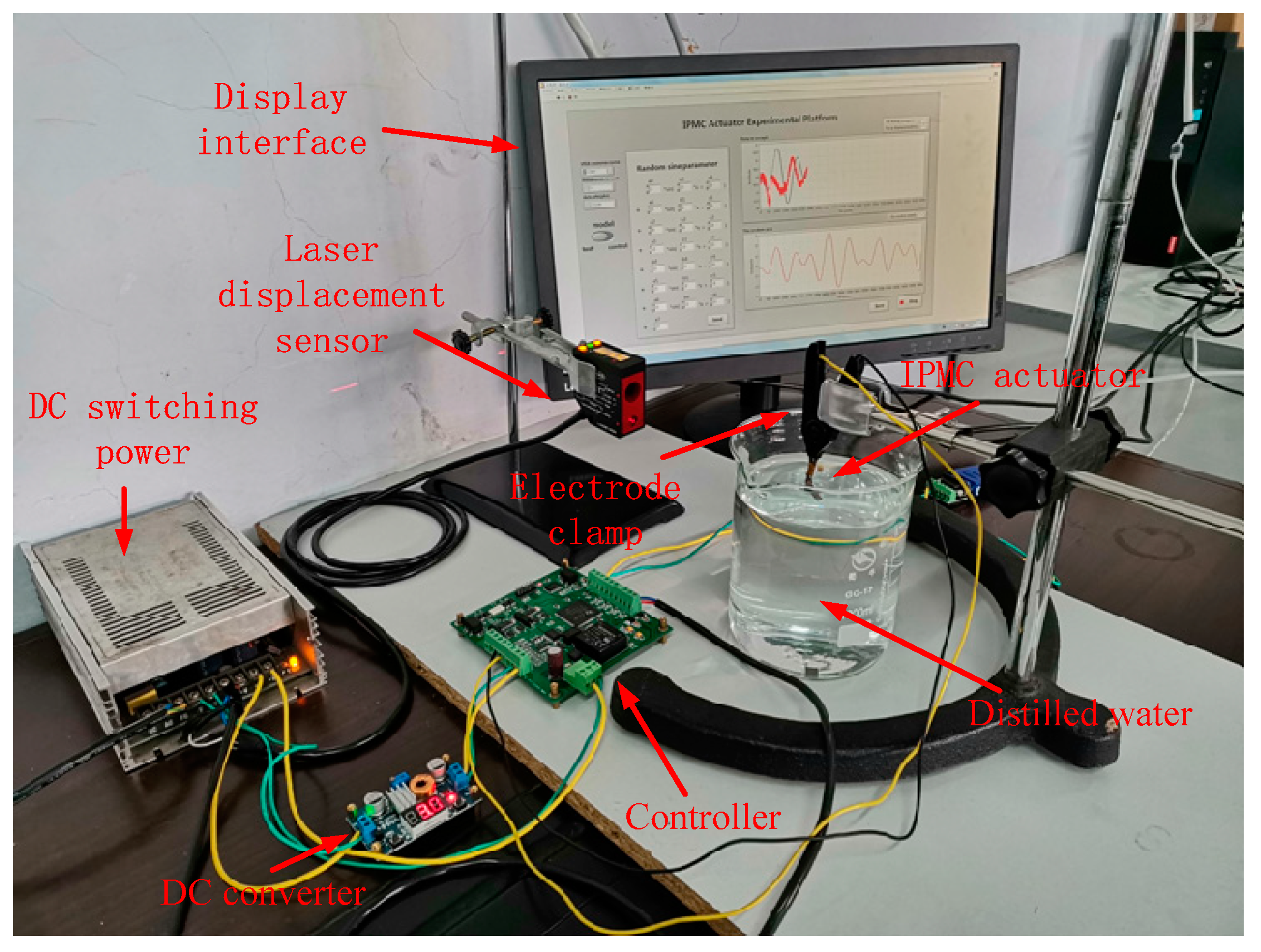
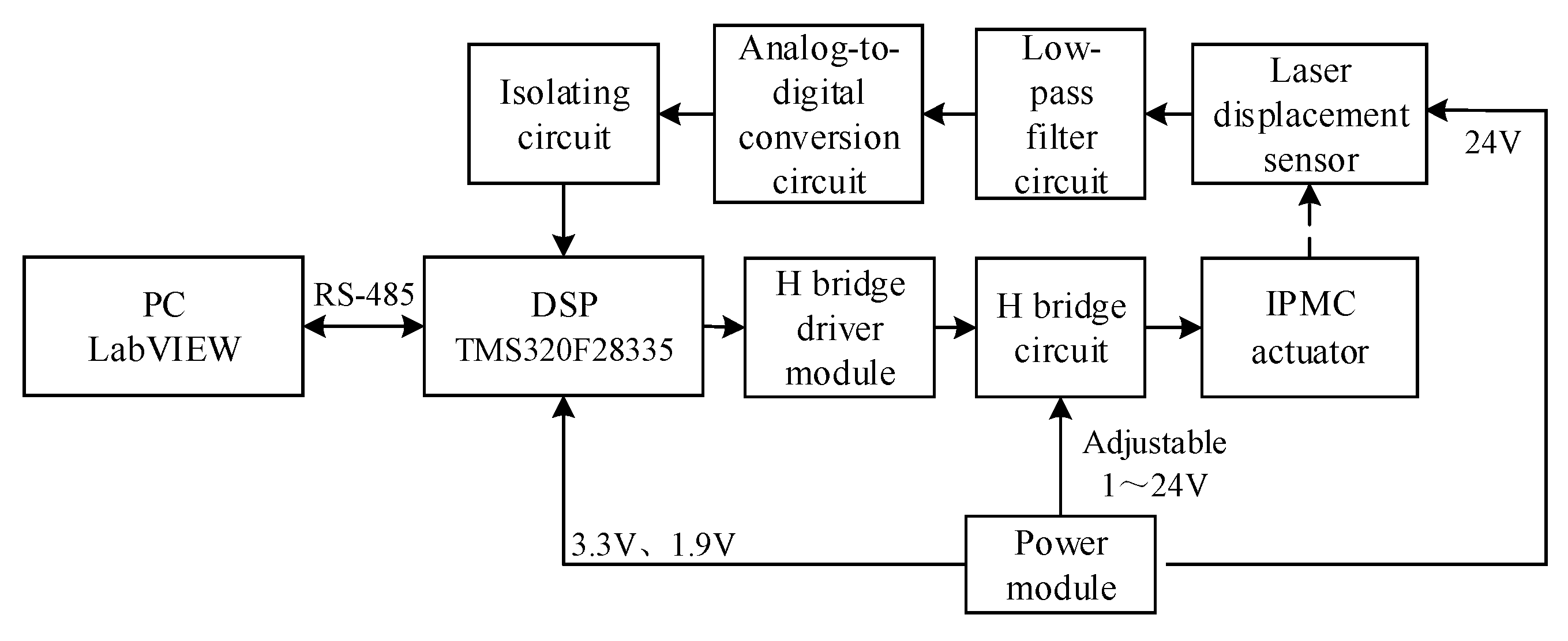
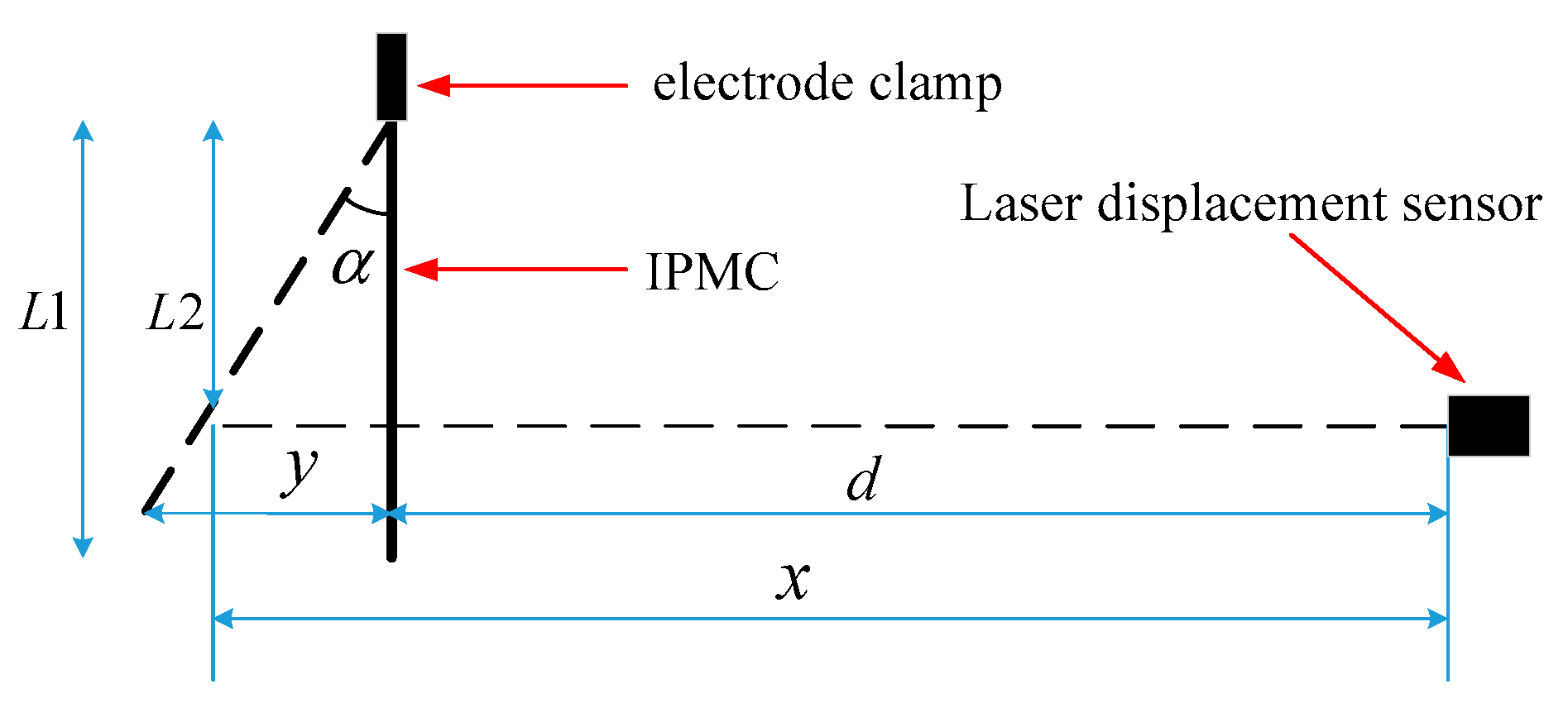
2.1. Testing Platform

Figure 2 shows the customized platform for the IPMC actuator. This platform allows testing and control of IPMC actuators. Specifically, an IPMC was immersed in distilled water and AC voltages with controllable amplitude and frequency were applied to the electrodes of the IPMC using a four-quadrant H-bridge circuit in order to drive the motion of the IPMC. Then, the tip displacement of the IPMC was measured using a high-precision laser displacement sensor (LE250; Banner Engineering Corp., Minneapolis, MN, USA) having a measuring accuracy of 0.04mm. Finally, the upper computer of the platform was established, and serial communication with the controller was achieved via the RS-485 bus to realize transmission, processing, and display of the control and experimental data of the platform.

Figure 3 shows the working principle of the platform. Instructions by the upper computer are transmitted to and processed by the main control chip (TMS320F28335) of the controller. The H-bridge driver module receives the CPU signals and drives H-bridge circuit to deliver the expected actuating voltage, and the IPMC generates displacement responses under stimulation by the actuating voltage. The displacement information detected by the laser displacement sensor is transmitted to the main control chip via a low-pass filter, an A/D converter, and an isolated circuit, and the main control chip transmits the data to the upper computer via serial communication for processing, display, and saving.

As the IPMC tip moves along an arc centered at the clamping end under voltage, the laser displacement sensor cannot directly measure the tip displacement of the IPMC actuator. Therefore, the returned data of the tip displacement is compensated by the upper computer, as shown in Figure 4. Here, $L1$ and $L2$ denote the length of the IPMC actuator and the initial distance from the laser point to the electrode clamp, respectively, d is the initial reading of the laser displacement sensor, $a$ is the angle between the dotted line position and the initial position of the IPMC actuator, $x$ is the reading of the displacement sensor when the IPMC is in the dotted line position, and y is the target value. These parameters can be calculated as

$$\begin{array}{l}y=L1\times \sin \left(\arctan \left((d-x)/L2\right)\right)\\ d-L1\times \sin \left(\arccos (L2/L1)\right)<x\le L1\times \sin \left(\arccos (L2/L1)\right)+d\end{array}$$

(1)

The testing results showed that the maximum deflection angle of the actuator exceeded 90° if the amplitude of the sinusoidal actuating voltage exceeded 3V. To guarantee the reliability of the collected data, the amplitude of the sinusoidal actuating voltage was kept below 3V during testing.

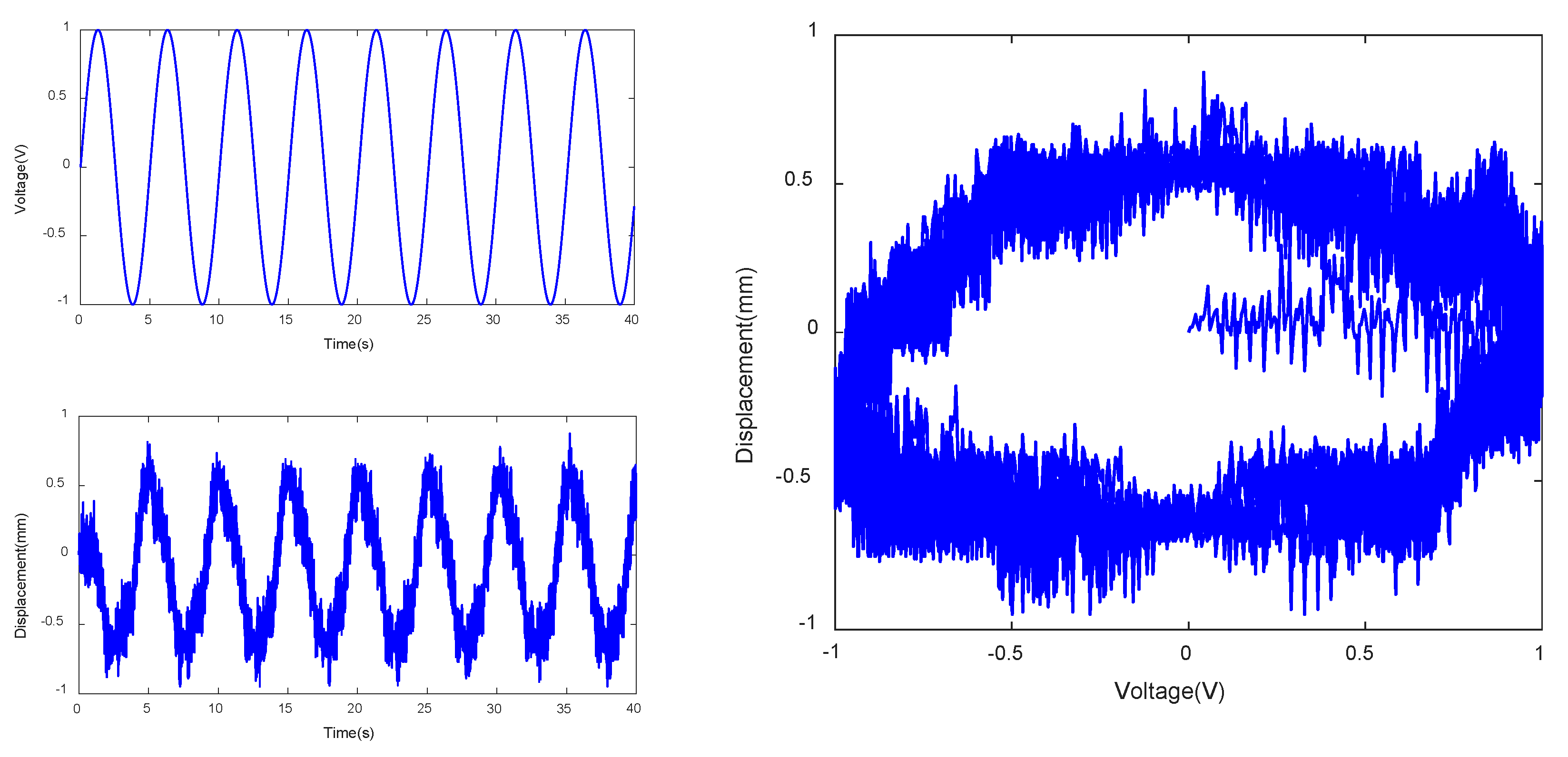
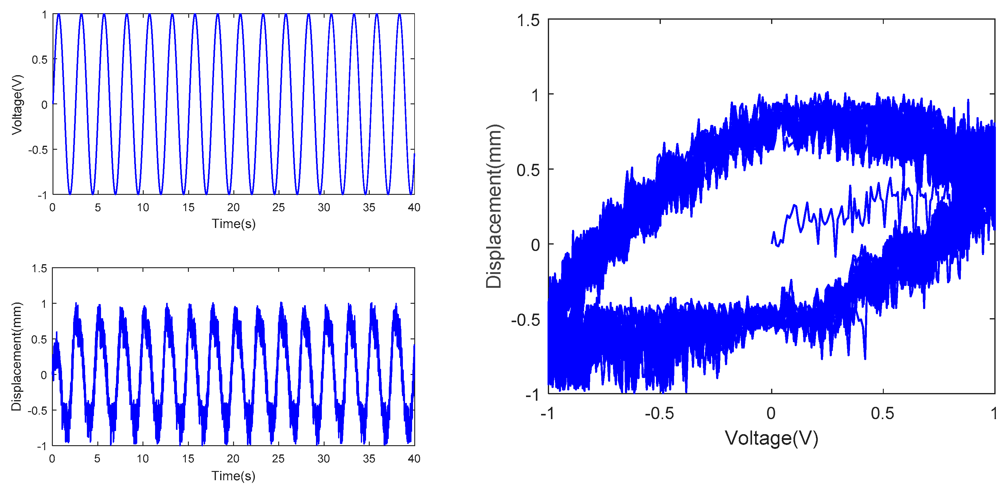
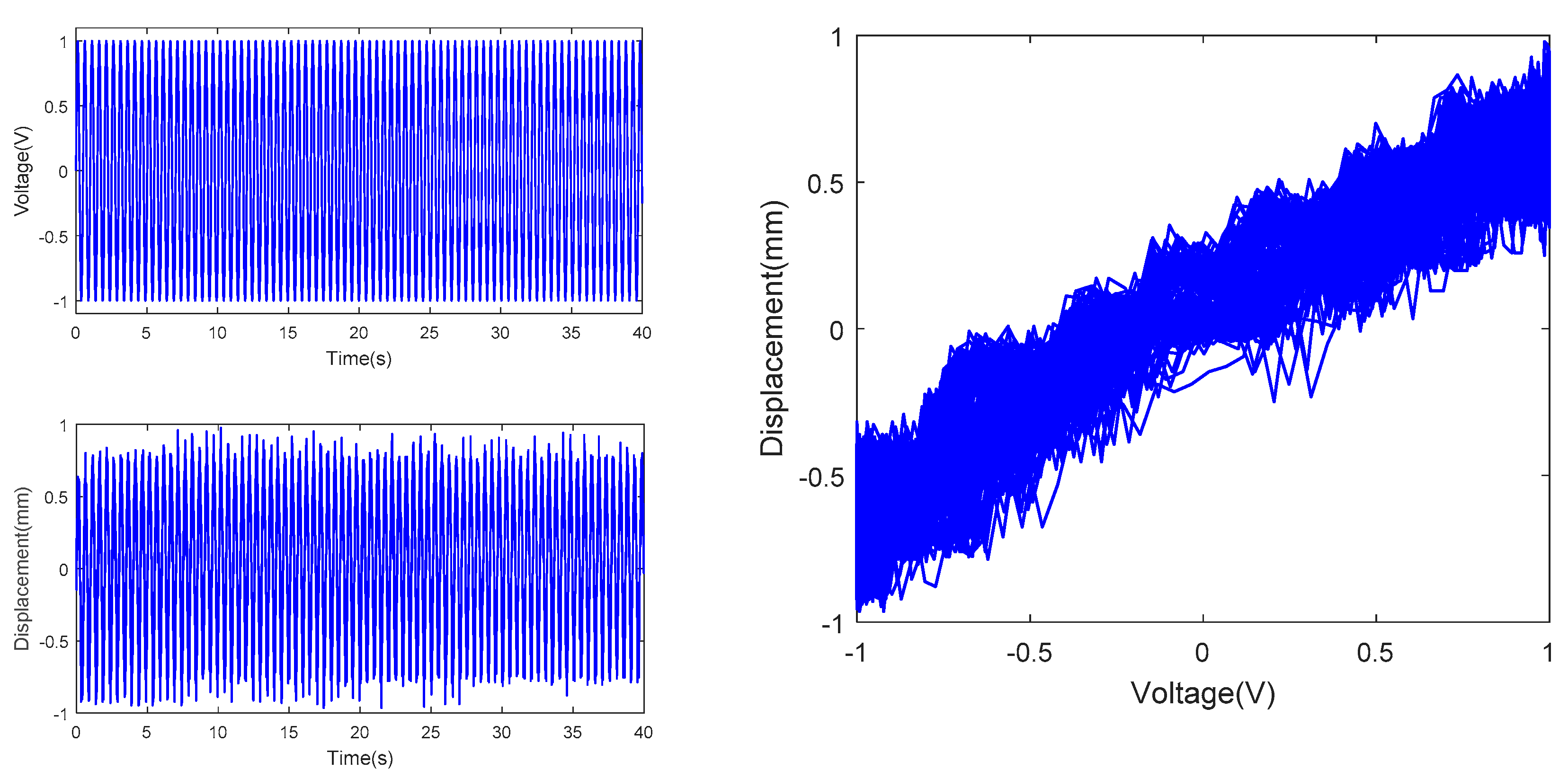
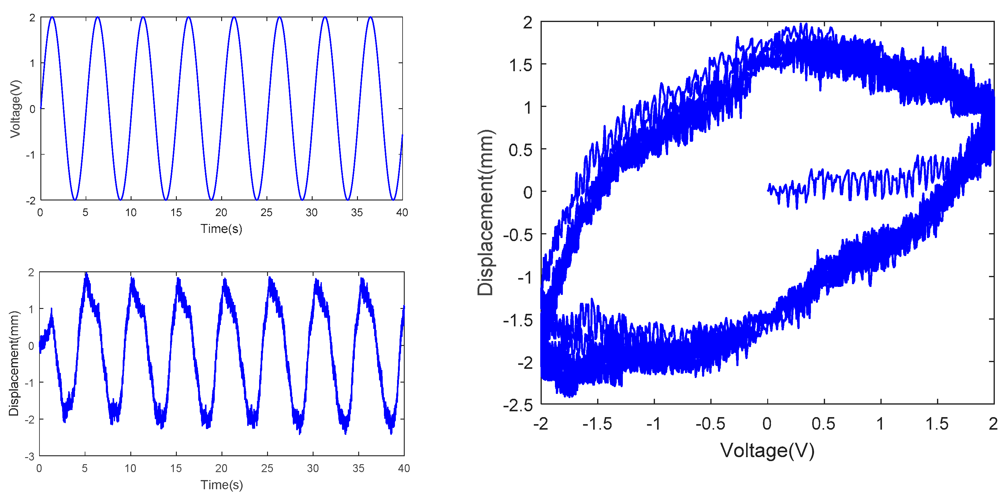
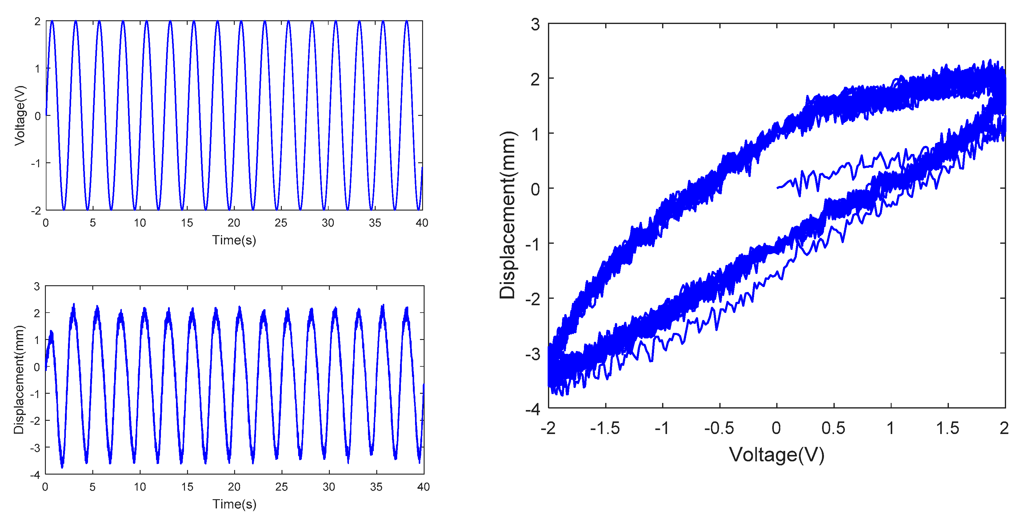
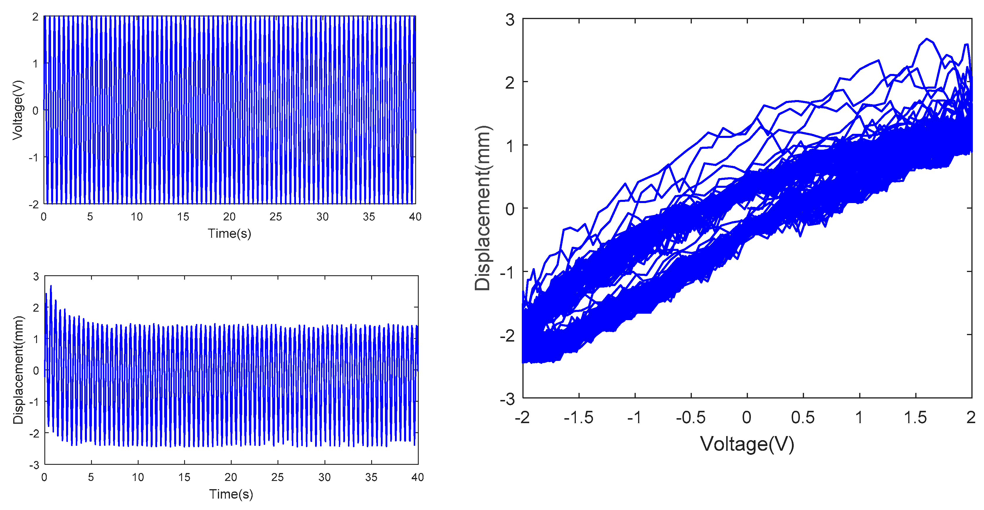
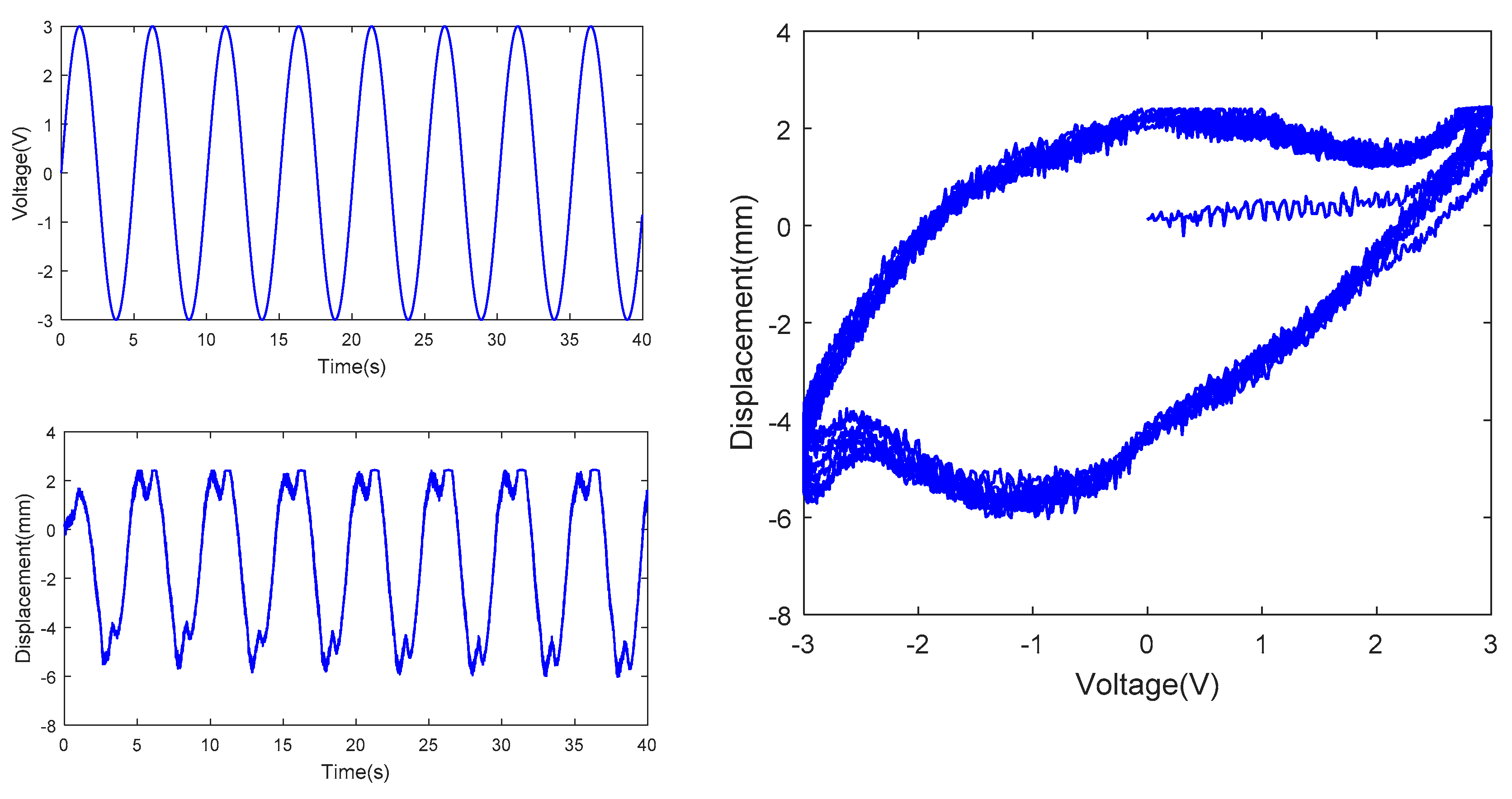
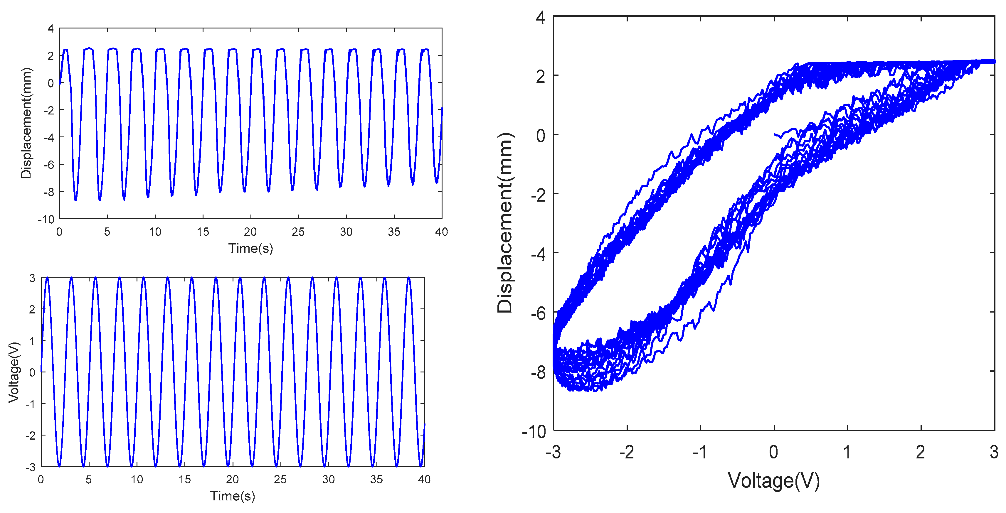
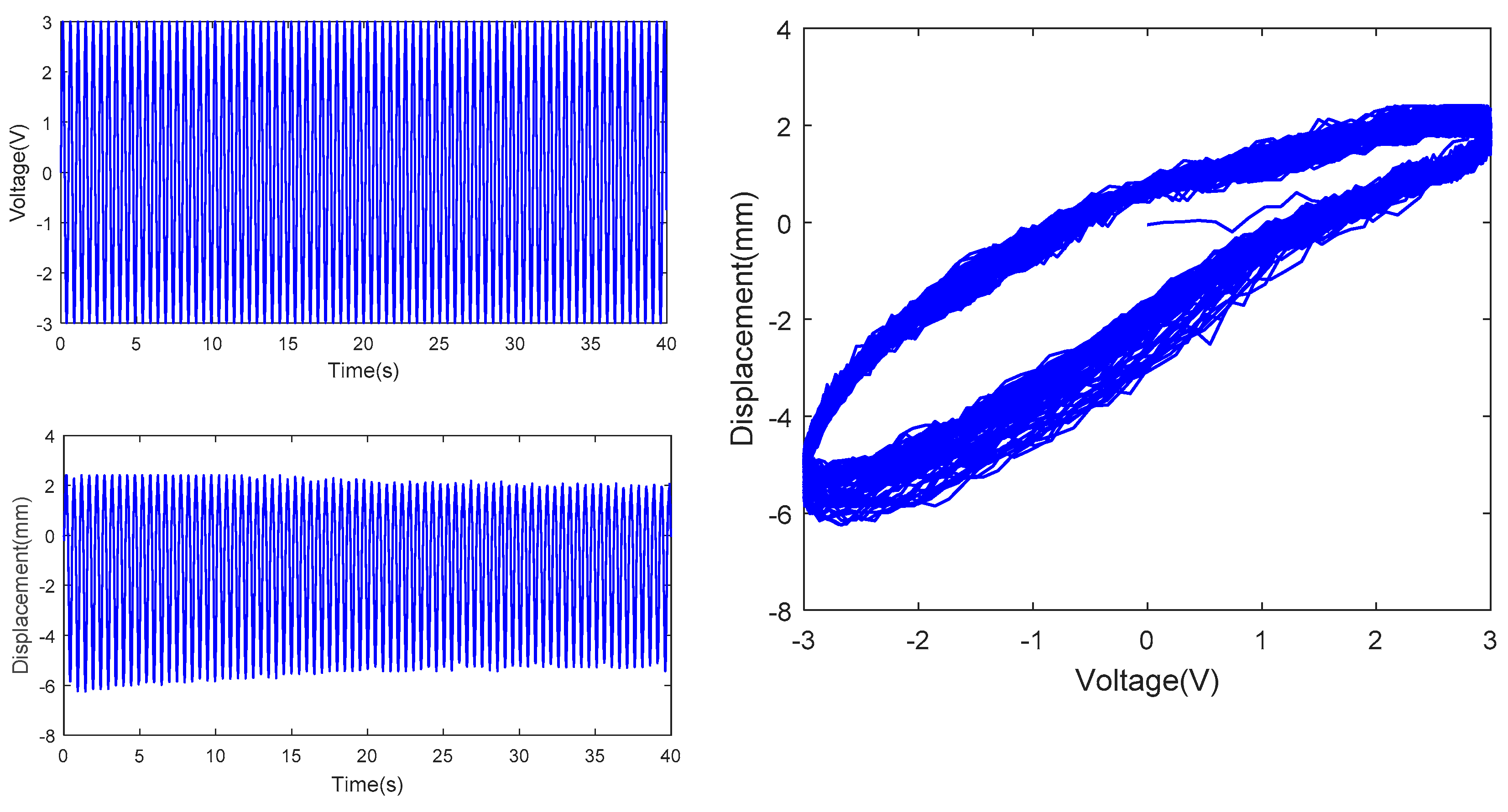
2.2. Testing of Hysteresis Characteristics

The amplitudes and frequencies of the sinusoidal AC voltages applied to the IPMC were 1V, 2V, and 3V and 0.5/2π Hz, 1/2π Hz, and 5/2π Hz, respectively. Figure 5, Figure 6, Figure 7, Figure 8, Figure 9, Figure 10, Figure 11, Figure 12, Figure 13, Figure 14, Figure 15 and Figure 16 show the tip displacements of different samples.

In the above figures, the top left subfigures of the figures are the actuating voltages of IPMC with different amplitude and frequency, the bottom left subfigures of the figures are the tip displacements of IPMC, and the right subfigures of the figures are the hysteresis curves combined by the actuating voltages and tip displacements;

Table 1. IPMCtip displacement range comparison table.

Amplitude of Actuating Voltage (V)	1			2			3
Frequency of actuating voltage (Hz)	0.5/2π	1/2π	5/2π	0.5/2π	1/2π	5/2π	0.5/2π	1/2π	5/2π
Lower limit of tip displacements (mm)	−0.9873	−1.1276	−1.1993	−2.5604	−3.9327	−2.487	−4.7787	−8.7983	−6.1326
Upper limit of tip displacements (mm)	0.8256	0.8923	0.8134	1.988	2.3796	2.7003	2.6328	2.5967	2.7528
Range of tip displacements (mm)	1.8129	2.0199	2.0127	4.5484	6.3123	5.1873	7.4115	11.395	8.8854

is the range comparison of IPMC tip displacement.

From Figures above and Table 1, under constant amplitude and varying frequency, delay of the IPMC displacement from the actuating voltage curve was observed, indicating hysteresis of the IPMC in terms of time. Meanwhile, the IPMC deformations at negative voltages were significantly larger than those at positive voltages. In addition, the actuating range of the IPMC actuator increased significantly with the frequency of the sinusoidal AC voltage, when the amplitude of sinusoidal voltage is 1V, 2V and 3V respectively, the range of tip displacement of IPMC increases by 0.207, 1.764 and 3.984, respectively, as the frequency rises from 0.5/2π Hz to 1/2πHz, while the range of tip displacement of IPMC increases by −0.007, −1.125, −2.510, respectively, as the frequency rises from 1/2π Hz to 5/2π Hz. Under constant frequency and varying amplitude, the overall IPMC deformation increased with the amplitude, when the amplitude is 3V, the range of tip displacement is much larger than that of 2V and 1V, resulting in improved actuating performance. Under constant amplitude and varying frequency, the tip displacement range was maximized, and the actuating performance was optimized at a frequency of 1/2π Hz. In summary, testing of the hysteresis characteristics of the IPMC revealed two features of the Pt-electrode IPMC in water:

1. Multiple mapping: For systems with hysteresis, a specific input may yield different outputs and a specific output may be attributed to different inputs.

2. Memory: For systems with hysteresis, the current output is determined not only by the current input but also historical signals and the varying trend.

3. Modeling of IPMC Actuator Based on Hysteresis Characteristics

Owing to the adverse effects of the hysteresis characteristics on the accuracy of IPMC control, considerable effort has been devoted toward establishing accurate and reliable mathematical models for the hysteresis characteristics of IPMC [46]. In this section, a least squares support vector machine-nonlinear autoregressive (LSSVM-NARX) model is proposed for the hysteresis characteristics of the Pt-electrode IPMC in water, and it is compared with the conventional Prandtl-Ishlinskii model. Furthermore, an artificial bee colony algorithm is developed to optimize the LSSVM-NARX model.

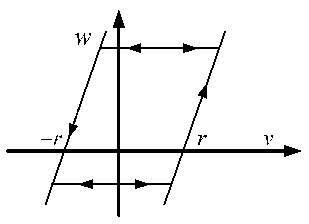
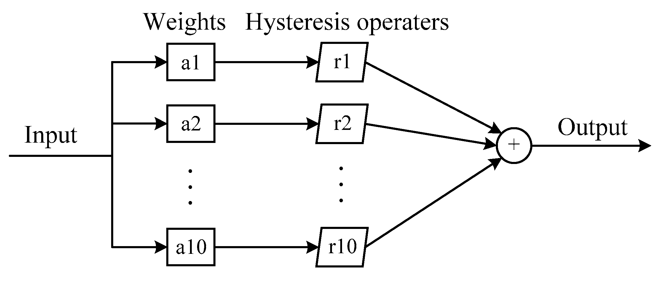
3.1. IPMC Actuator Modeling Based on Prandtl-Ishlinskii Method

The Prandtl-Ishlinskii model has been widely used for the modeling and compensation of hysteresis nonlinearity. A typical Prandtl-Ishlinskii model consists of a play hysteresis operator and a density function [47]. The play hysteresis operator of the Prandtl-Ishlinskii model is continuous and rate independent [48]; the Schematic diagram is shown in Figure 14. Suppose that $C_m[0,t_E]$ represents a piecewise monotone continuous space, if any input $v(t)\in C_m[0,t_E]$ is monotonic ($0=t_0<t_1<\dots <t_N=t_E$) on any subinterval $[t_i,t_{i+1}]$ of the time variable $[0,t_N]$, the play hysteresis operator is expressed as follows:

$$\begin{array}{c}{F}_r[v](0)=f_r\left(v(0),0\right)=w(0)\\ F_r[v](t)=f_r\left(v(t),F_r[v](t_i)\right),t_i<t\le t_{i+1}且0\le i\le N-1\\ f_r(v,w)=\max \left(v-r,\min (v+r,w)\right)\end{array}$$

(2)

where the characteristic parameters of the Play hysteresis operator are input $v$ and threshold $r$.

Figure 15 shows the structure of the proposed Prandtl-Ishlinskii model. This model was obtained by the weighted sum of 10 play hysteresis operators. Here, a1-a10 and r1-r10 denote the weighted values and thresholds of the operators, respectively. These variables, which are the parameters of the Prandtl-Ishlinskii model, are usually obtained using optimization algorithms. In this study, the parameters were determined using PSO.

The procedure of PSO is as follows:

I. Initialization of particle swarms: 100particleswith a dimension of 20, including the number of particle swarms, random position, and speed of particles, are initialized.

II. Calculation of fitness of each particle:

$$\mathrm{fitness}=\sqrt{\frac{{\displaystyle \sum {(Y_{test}-Y_1)}^2}}{l_{test}}}$$

(3)

where $Y_{test}$ is the experimental data, $Y_1$ is the output calculated on the basis if the optimized parameters, and $l_{test}$ is the number of experimental data.

III. Recording of optimized position of each particle: For each particle, the current position is regarded as the optimized position if its fitness exceeds that of the previous optimized position.

IV. Recording of optimized position of particle swarm: For each particle, the fitness of the global optimized position is replaced by that of the current position if the latter exceeds the former.

V. The speed and position of the particle are updated as:

$$v_{i,j}\left(t1+1\right)=w^{\prime }{v}_{i,j}(t1)+c_1{r}_1[p_{i,j}-x_{i,j}(t1)]+c_2{r}_2[p_{g,j}-x_{i,j}(t1)]$$

(4)

where the inertial weight is used as the weighting factor ($w^{\prime }$), $c_i$ and $r_i$ are constants, and $p_{i,j}$ is the current position.

The weight is updated by

$$w^{\prime }={w^{\prime }}_{\max }-\frac{t1\times ({w^{\prime }}_{\max }-{w^{\prime }}_{\min })}{t{1}_{\max }}$$

(5)

The position is updated by

$$x_{i,j}(t1+1)=x_{i,j}(t1)+v_{i,j}(t1+1),j=1$$

(6)

VI. Obtain the results: The optimization ends if the number of iterations reaches its maximum value (100) or the fitness reaches the prescribed value.

Owing to the symmetry of play hysteresis operators, the Prandtl-Ishlinskii model was obtained by recognition of the tip displacement data at an actuating voltage with an amplitude of 3V and frequency of 1/2π Hz by PSO. The 20parameters are summarized in

Table 2. Parameters of Prandtl-Ishlinskii model.

	a1	a2	a3	a4	a5	a6	a7	a8	a9	a10
Value	2.446	−8.8831	−2.5468	−5.3785	7.4586	−8.13	3.711	4.986	2.3852	10
	r1	r2	r3	r4	r5	r6	r7	r8	r9	r10
Value	4.2268	−10	−4.2276	2.6812	6.3775	10	−7.9211	10	−10	−3.8301

.

The Prandtl-Ishlinskii model was verified using the tip displacement data obtained at two sinusoidal actuating voltages which one voltage is an amplitude of 2V and a frequency of 1/2π Hz and another voltage is an amplitude of 3V and a frequency 5/2π Hz. The results of one period of two sinusoidal actuating voltages are shown in Figure 16; Figure 17. Here, the blue solid line and the red dotted line represent the tip displacements obtained experimentally and by the Prandtl-Ishlinskii model, respectively. The errors of the Prandtl-Ishlinskii model at two sinusoidal actuating voltages are shown in Figure 18 and Figure 19, the root mean square errors (RMSE) are 0.5685 and 0.8345. These curves are not consistent, indicating severe modeling errors. The maximum absolute value of the error of the Prandtl-Ishlinskii model exceeded 1.5 and the errors were widely distributed.

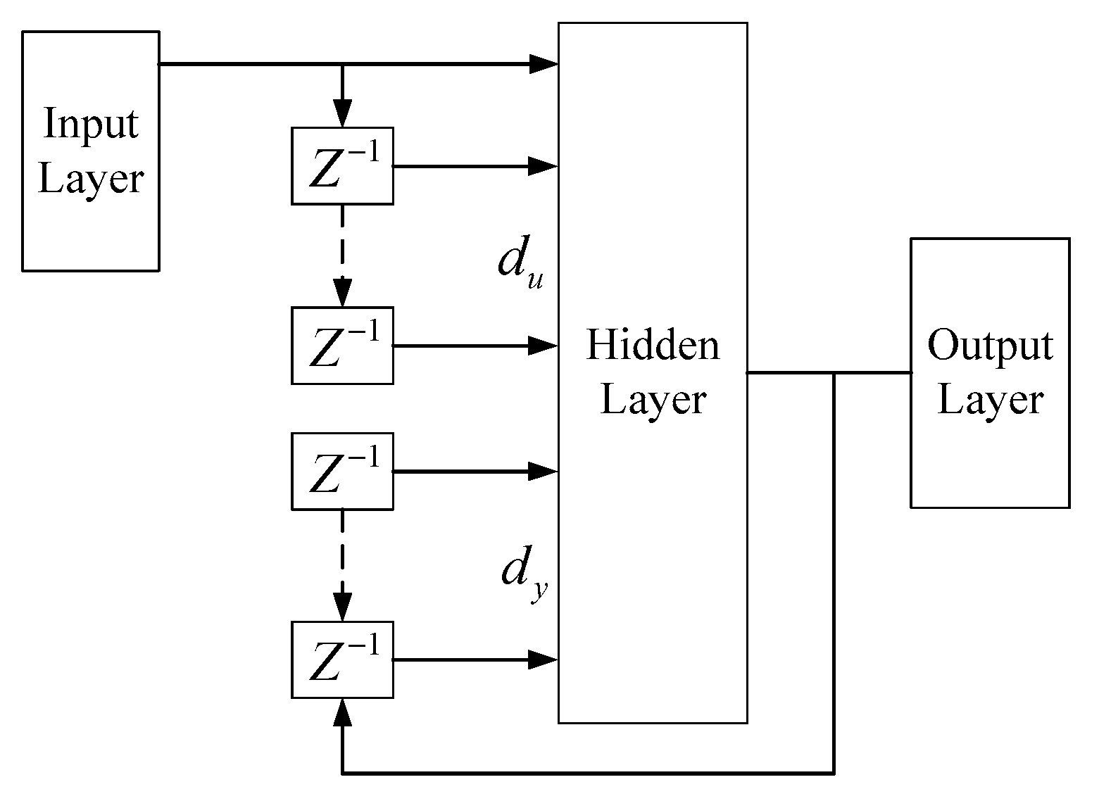
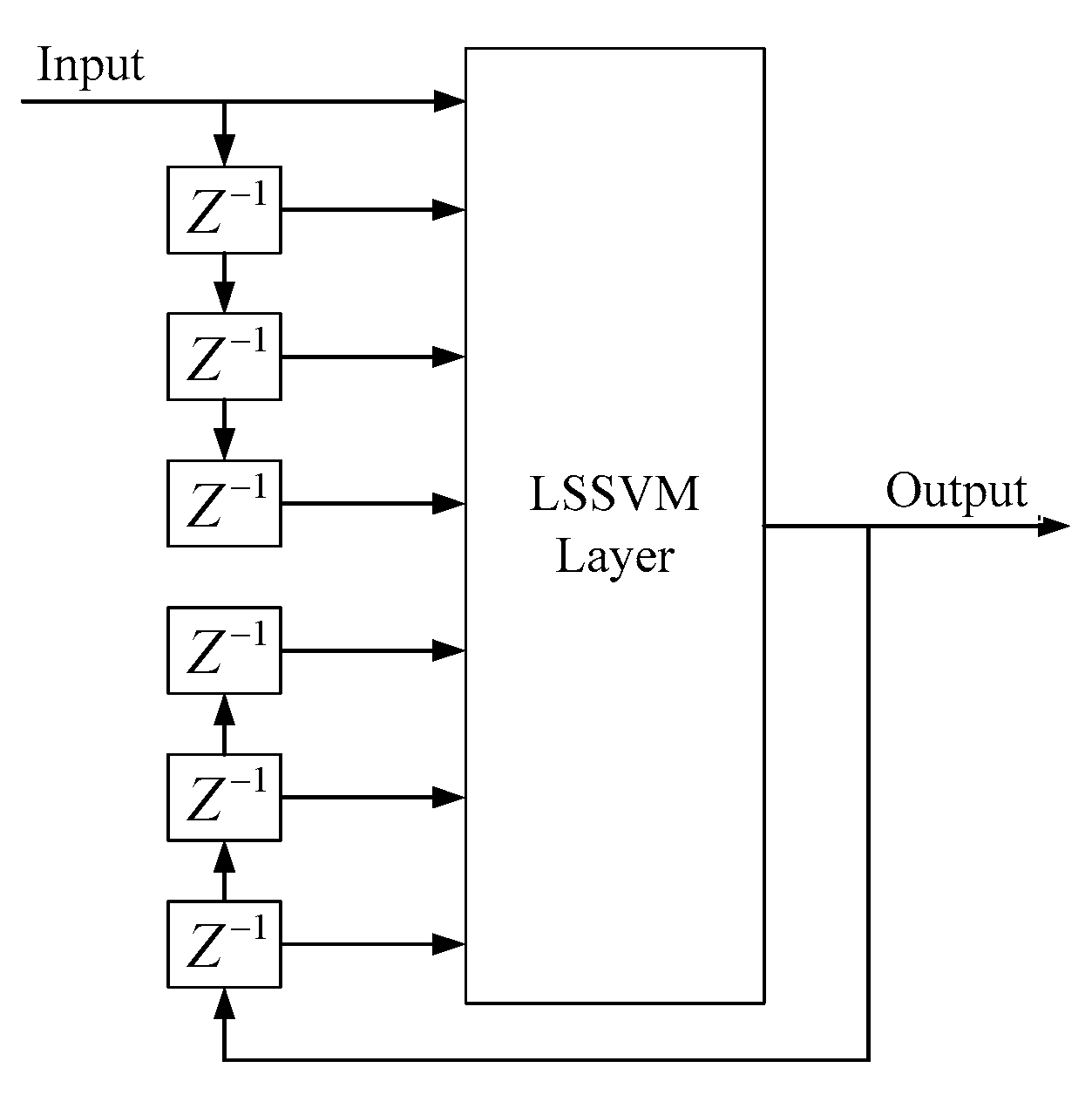
3.2. Modeling of IPMC Actuators Based on the LSSVM-NARX Method

NARX is a dynamic neural network with excellent nonlinearity mapping capability. The concept of the dynamic autoregressive time sequence has been introduced into NARX. Hence, NARX exhibits good interference resistance and dynamic features in predictions of issues involving time sequences [49,50,51,52]. The mathematical equation of NARX is

$$y(n+1)=f\left[\begin{array}{c}y(n),y(n-1),\dots y(n-d_y+1),\\ u(n),u(n-1),\dots u(n-d_u+1)\end{array}\right]$$

(7)

where y(n) and u(n) are the output and input at moment n, respectively, while d_y and d_u are the output and input delays, respectively. In NARX, the current output is determined by not only the current input but also the delay d_u of the current input and delay d_u of the output. The weight parameters of the neural network can be continuously adjusted by learning the nonlinearity of these data so that the prediction of future parameters can be achieved.

Figure 20 shows the structure of NARX, $Z^{-1}$ is the delay operator in picture. Like neural networks, NARX consists of an input layer, a hidden layer, and an output layer. However, NARX involves analysis of the input and output delays. The prediction accuracy is proportional to the delay; however, an increase in the delay leads to increased calculation. Hence, the delay is determined by optimization of the accuracy and efficiency.

As a modification of SVM, LSSVM exhibits significantly higher calculation speed and lower complexity [53,54,55]. In general, LSSVM is applicable only to issues involving single mapping of input and output. Hence, multiple mapping in hysteresis characteristics is converted into single mapping in the modeling. In the NARX model, the input and output at the previous moment are used as the reference input in the current moment. This feature overcomes the limitation of LSSVM in issues involving multiple mapping.

A regression model was established on the basis of the structure of the NARX model:

$$h_k=f(x_k)+{\xi }_k$$

(8)

where $x_k=\left[u_k,\dots ,u_{k-m},y_{k-1},\dots y_{k-n}\right]$, $u_k$ and $y_k$ are the input voltage and output displacement at moment $k$, respectively, ${\xi }_k$ is the prediction error, and f(∙)denotes the nonlinear regressive model. In addition, m ≥ 0 and n ≥ 0 denote the regression orders of the model.

It has been shown that the input data are mapped to a high-dimensional feature space in LSSVM, followed by the development of a linear regressive function. The hysteresis characteristics of the IPMC were modeled using LSSVM. Here, f(∙) is as follows:

$$h(x)={\omega }^{\mathrm{T}}\phi (x)+b$$

(9)

where the input is mapped to a high-dimensional space by the nonlinear function $\phi (x)$,${\left\{x_k,h_k\right\}}_{k=1}^N$ is the given training set, and N is the number of training samples. Furthermore, ω and b are the weight vector and error, respectively, and they can be determined by

$$\{\begin{array}{c}\underset{\omega ,\xi ,b}{\min }J(\omega ,\xi )=\frac{1}{2}{\omega }^{\mathrm{T}}\omega +\frac{1}{2}C{\displaystyle \sum _{k=1}^N{\xi }_k^2}\\ y_k= {\omega }^{\mathrm{T}}\phi (x_k)+b+{\xi }_k^{}\end{array}$$

(10)

where $C$ is the regularization factor balancing the training error and the model complexity. The Lagrangian function can be expressed as

$$L(\omega ,b,\xi ,\beta )=J(\omega ,\xi )-{\displaystyle \sum _{k-1}^N{\alpha }_k\left[{\omega }^{\mathrm{T}}\phi (x_k)+b+{\xi }_k-h_k\right]}$$

(11)

where ${\alpha }_k$ denotes the Lagrangian factor. The optimized solutions meet the following requirements:

$$\{\begin{array}{c}\frac{\partial L}{\partial \omega }=0\to \omega ={\displaystyle \sum _{k=1}^N{\alpha }_k\phi (x_k)}\\ \frac{\partial L}{\partial {\xi }_k}=0\to {\alpha }_k=C{\xi }_k\\ \frac{\partial L}{\partial b}=0\to {\displaystyle \sum _{k=1}^N{\alpha }_k=0}\\ \frac{\partial L}{{\alpha }_k}=0\to {\omega }^{\mathrm{T}}\phi (x)+b+{\xi }_k-h_k=0\end{array}$$

(12)

In LSSVM, regression is regarded as an optimization problem in the initial weight space. The optimized conditions are determined by solving a series of partial derivatives. The dual function established on the basis of these partial derivatives is

$$\left[\begin{array}{cc}0& e_{N\times 1}^{\mathrm{T}}\\ e_{N\times 1}^{}& \mathsf{\Omega }+I_N/C\end{array}\right]\left[\begin{array}{c}b\\ \alpha \end{array}\right]=\left[\begin{array}{c}0\\ H\end{array}\right]$$

(13)

where $e_{N\times 1}^{}=\left[1;1;\dots ;1\right]$, $\alpha =\left[{\alpha }_1;{\alpha }_2;\dots ;{\alpha }_N\right]$, $H=\left[h_1;h_2;\dots ;h_N\right]$, $I_N$ is a unit matrix, ${\mathsf{\Omega }}_{ij}={\phi }^{\mathrm{T}}(x_i)·\phi (x_j)=K(x_i,x_j)$, and $K(\cdot )$ is a radial basis kernel function:

$$K(x_i,x_j)=\exp (-{\Vert x_i-x_j\Vert }^2/2{\sigma }^2)$$

(14)

where $\sigma >0$ is the bandwidth parameter of the kernel function.

Furthermore, $\sigma$ and $b$ can be obtained by Equation (11), and the LSSVM-NARX regressive model is given by

$$y_k=h(x)={\displaystyle \sum _{k=1}^N{\alpha }_{k}K(x,x_k)}+b$$

(15)

Figure 21 shows the structure of the LSSVM-NARX model. In addition to the existing input, three delays of the initial input and the output were introduced to overcome the limitation of the LSSVM model in issues involving multiple mapping of input and output.

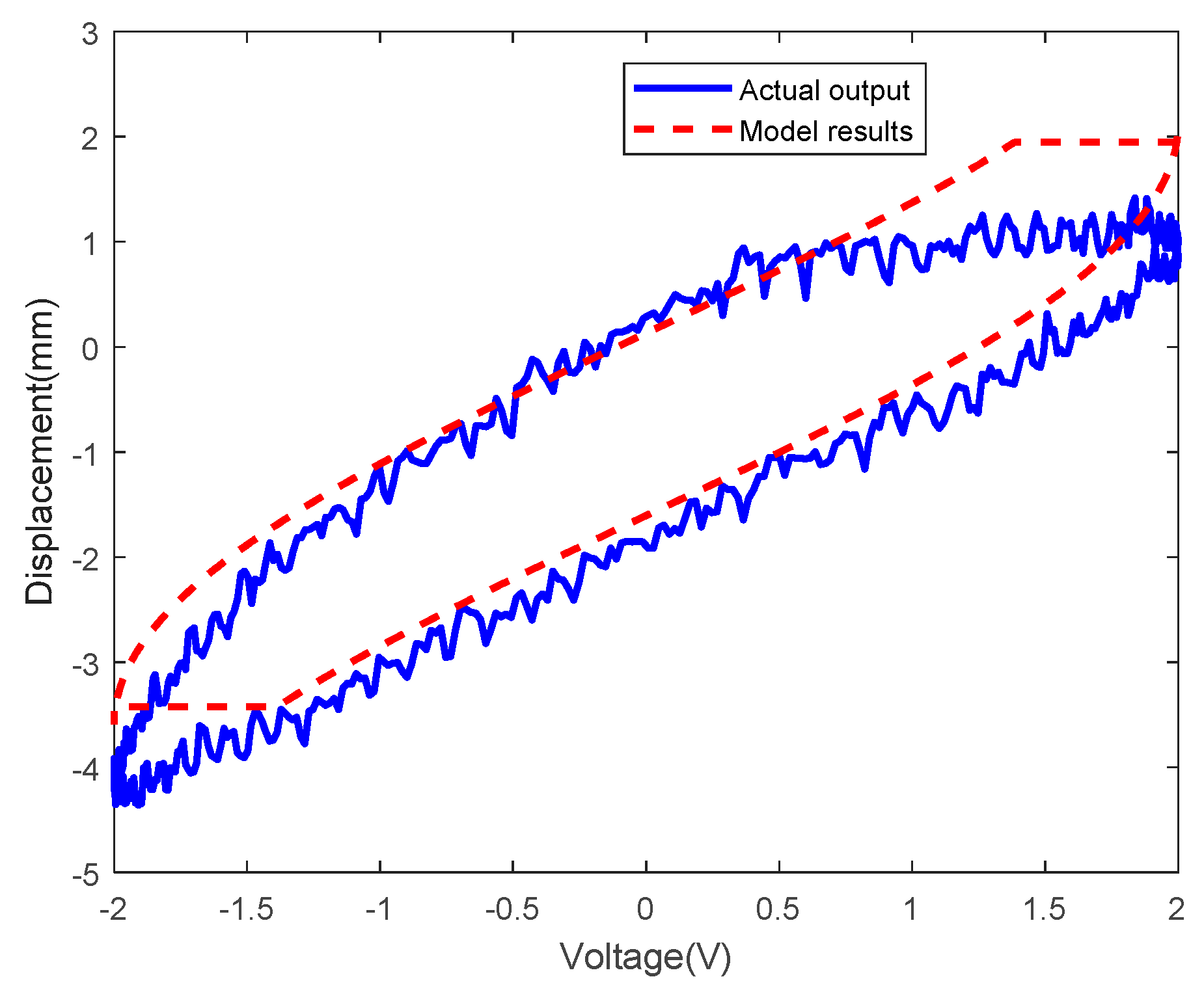
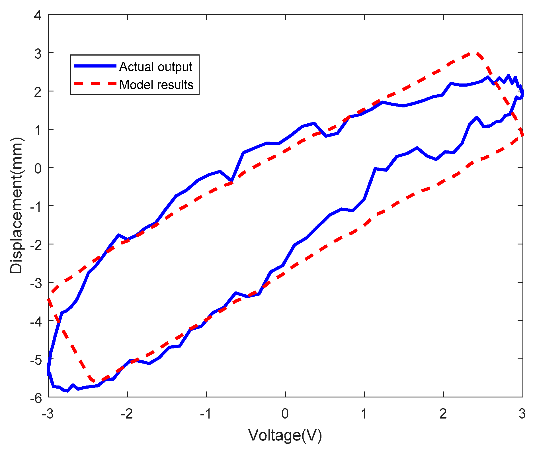
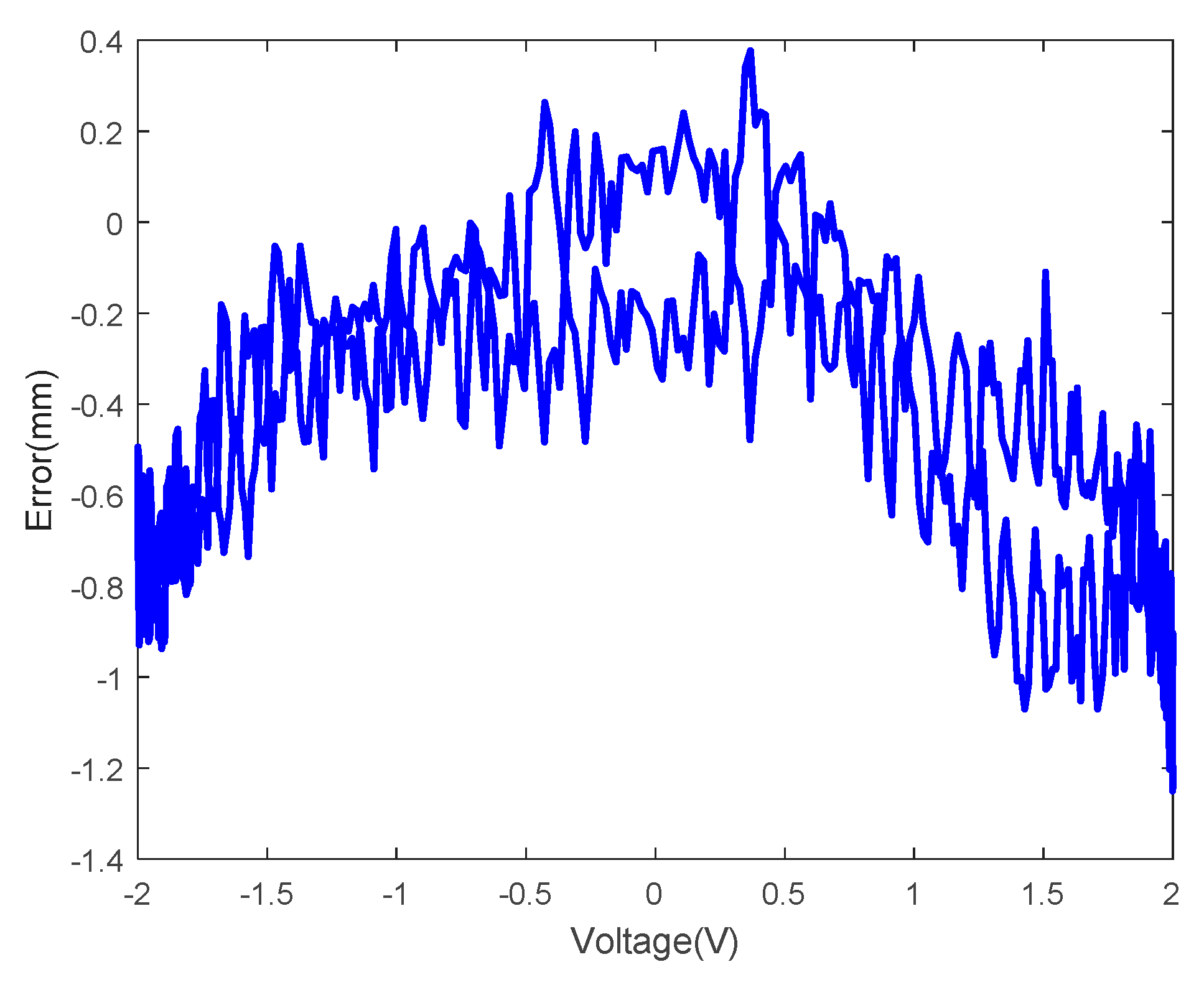
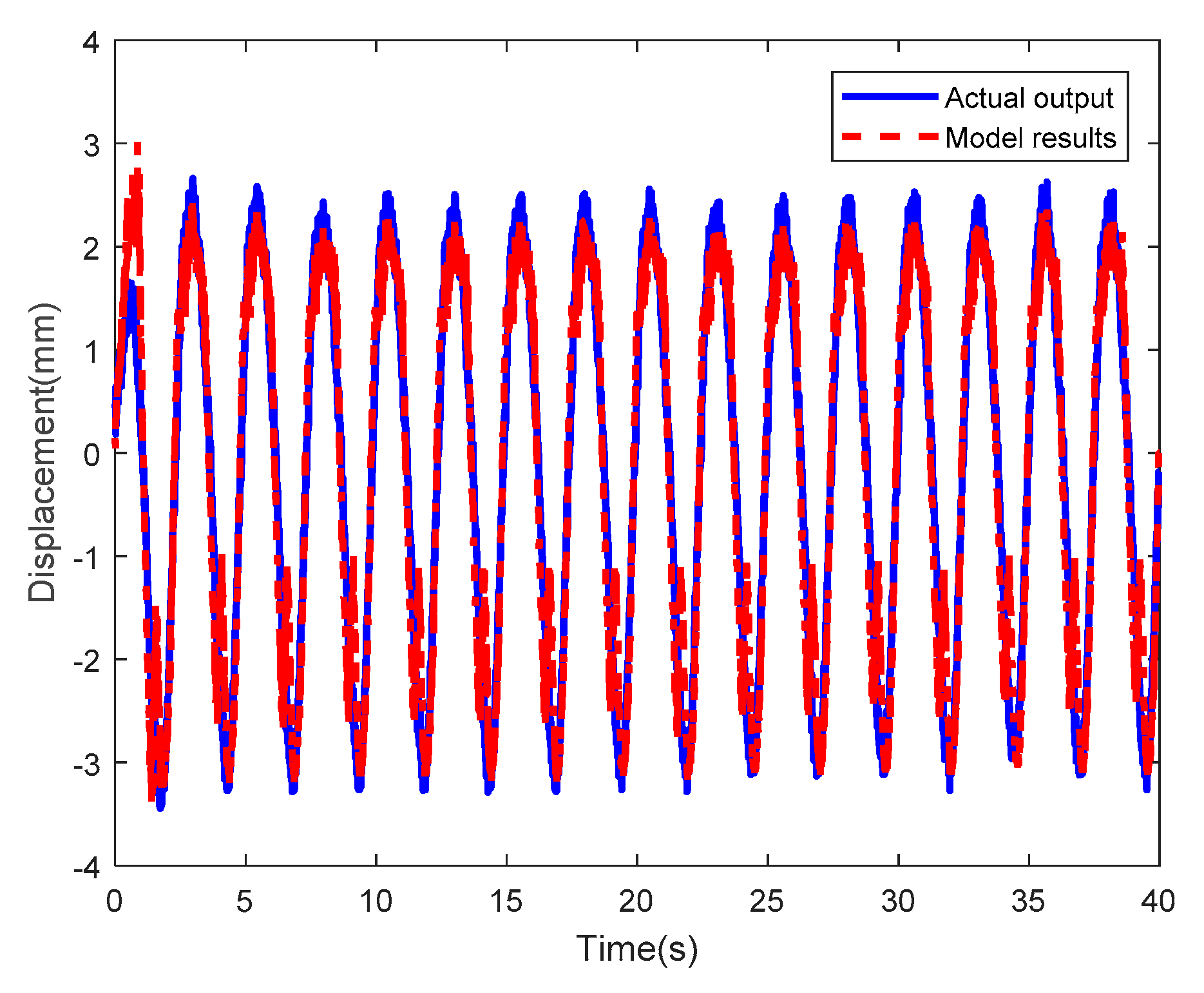
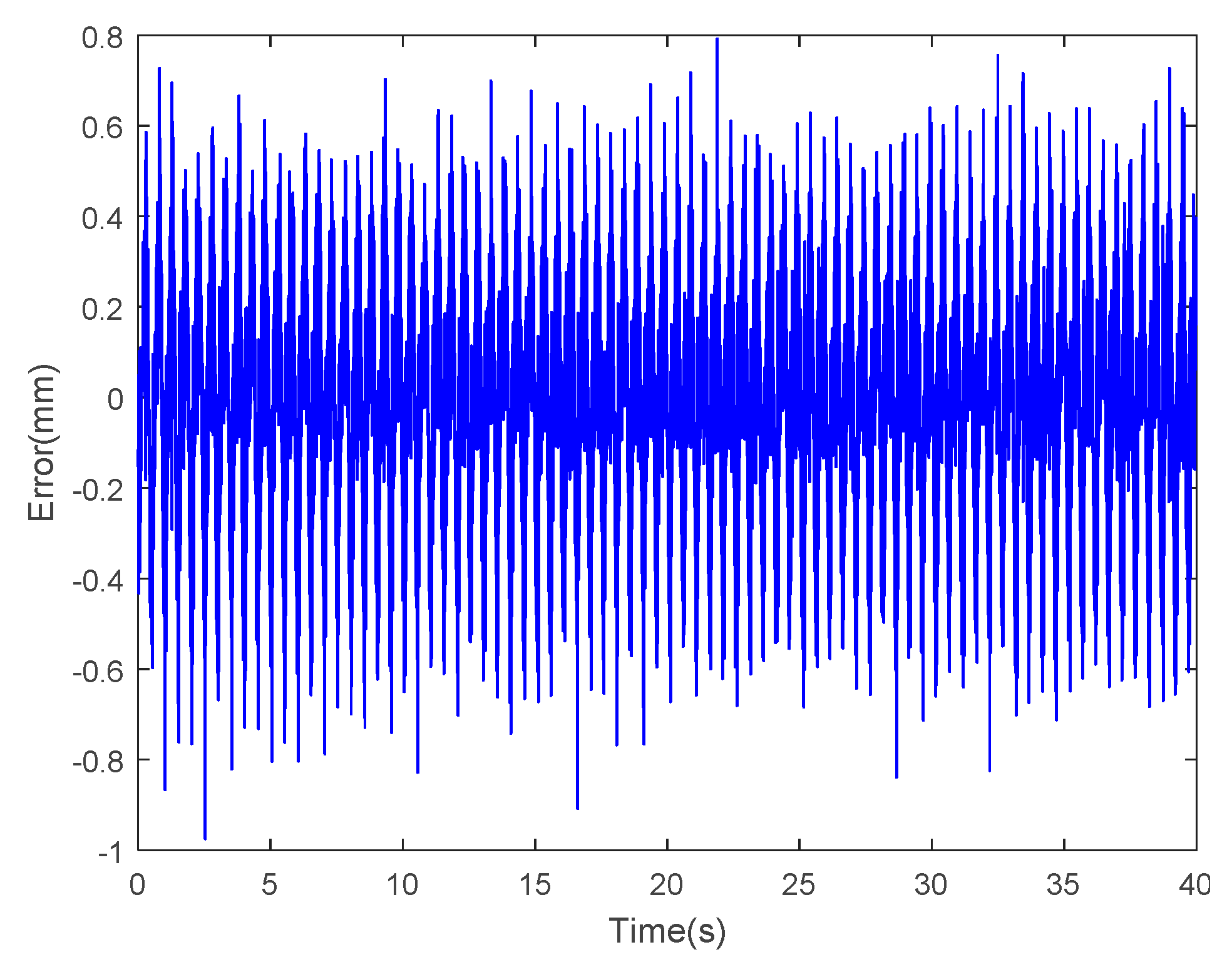
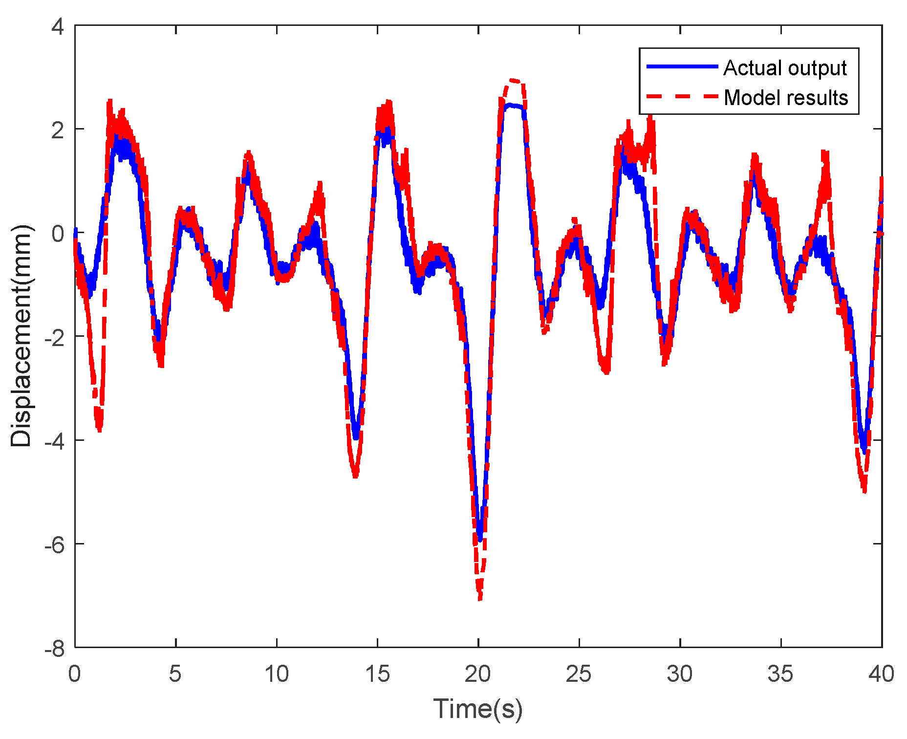
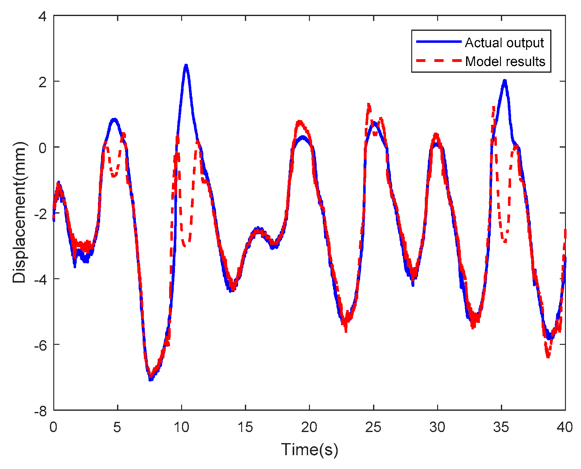
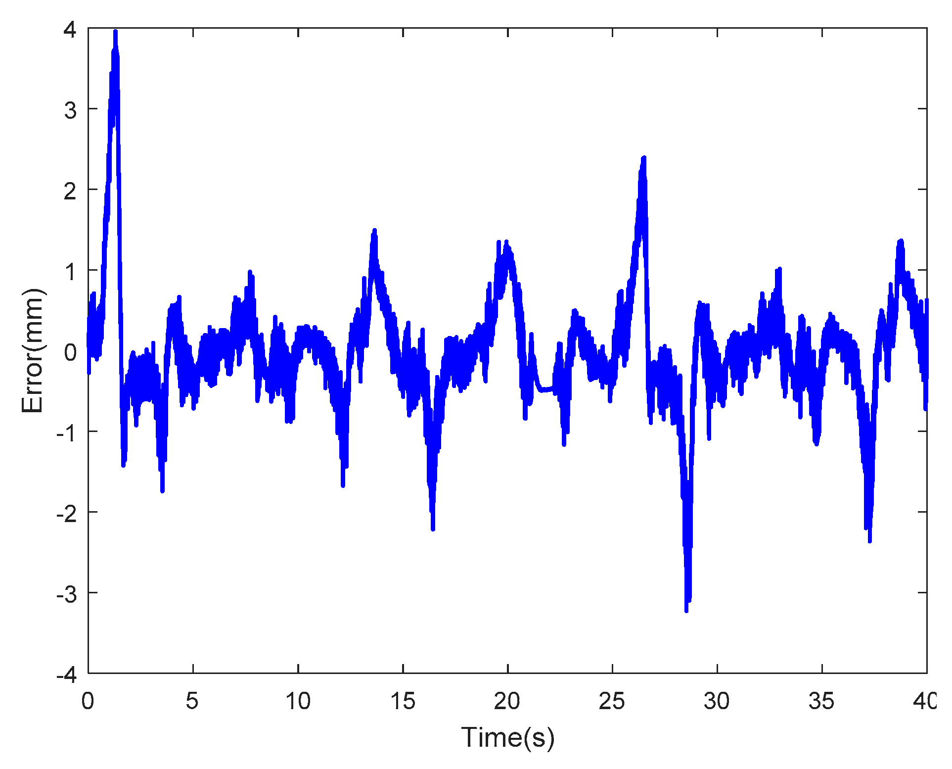
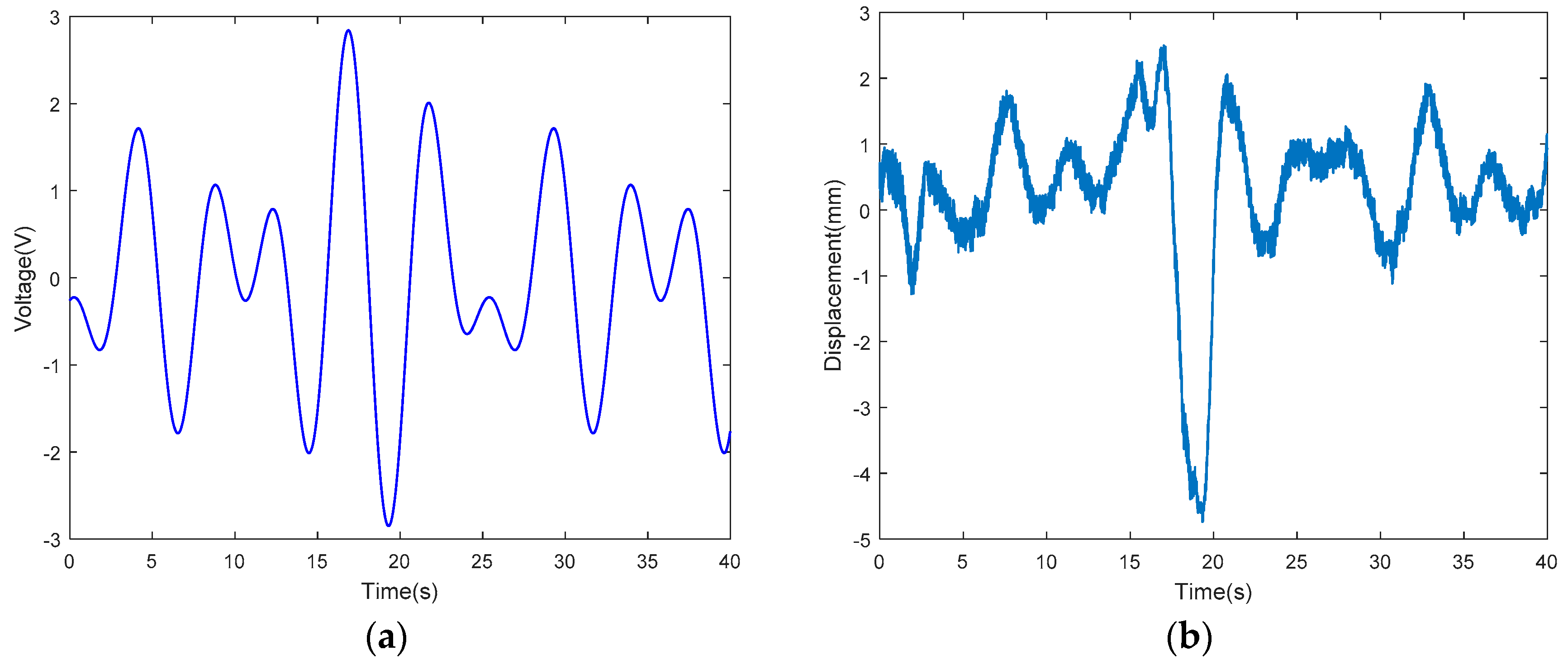
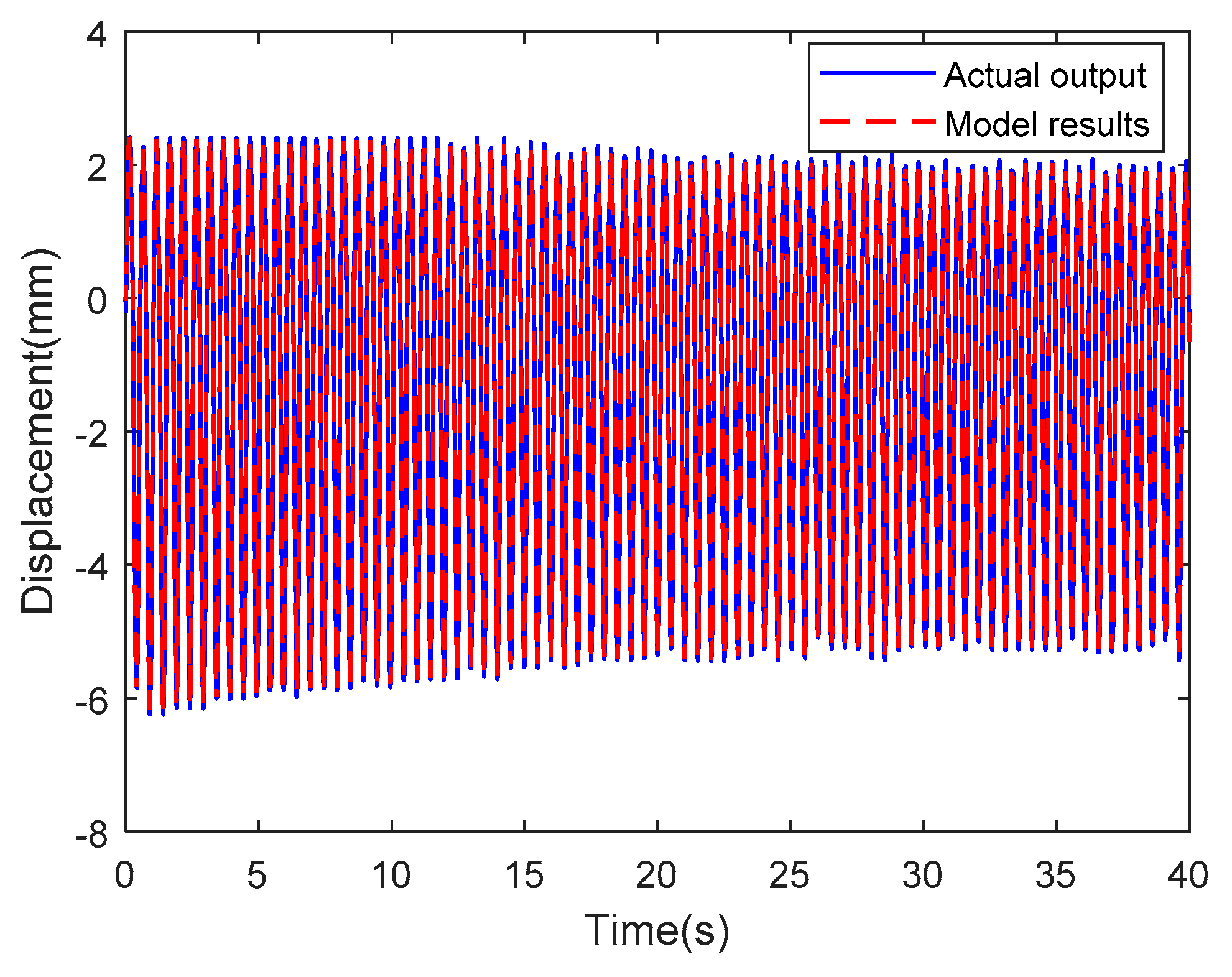
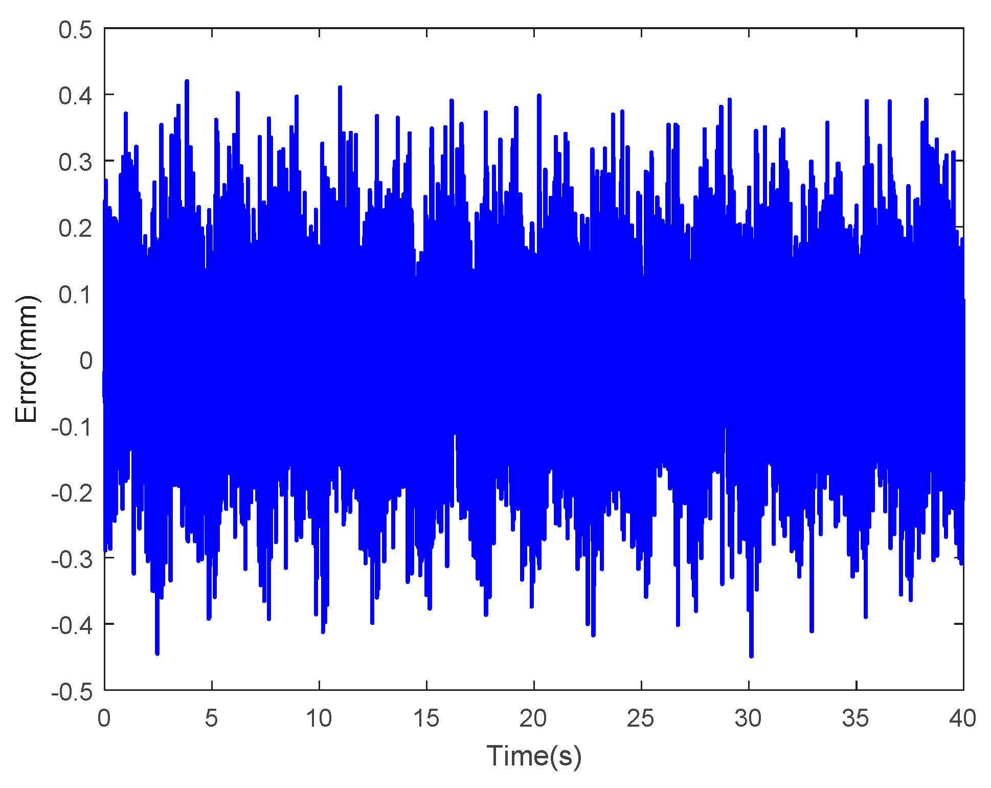
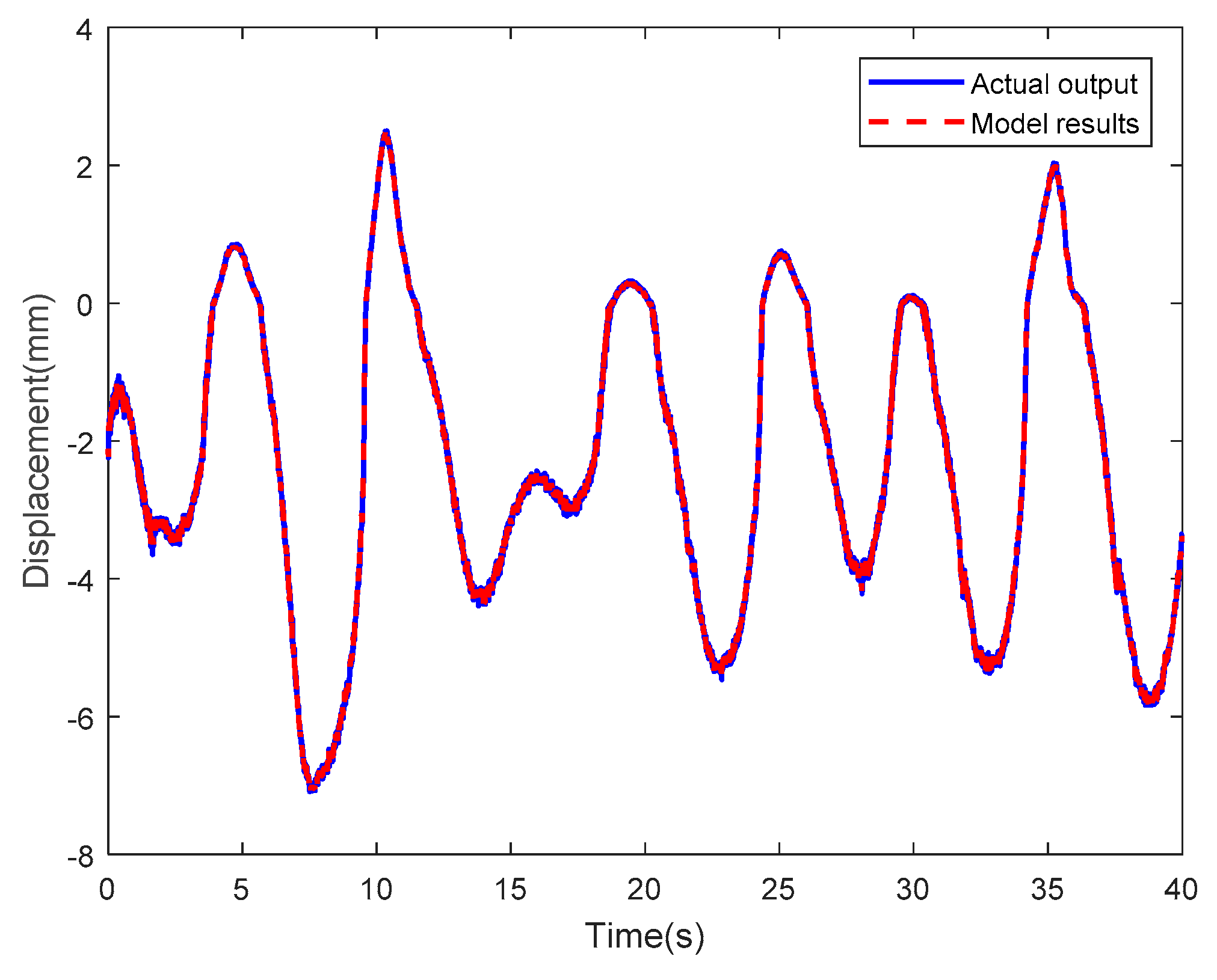
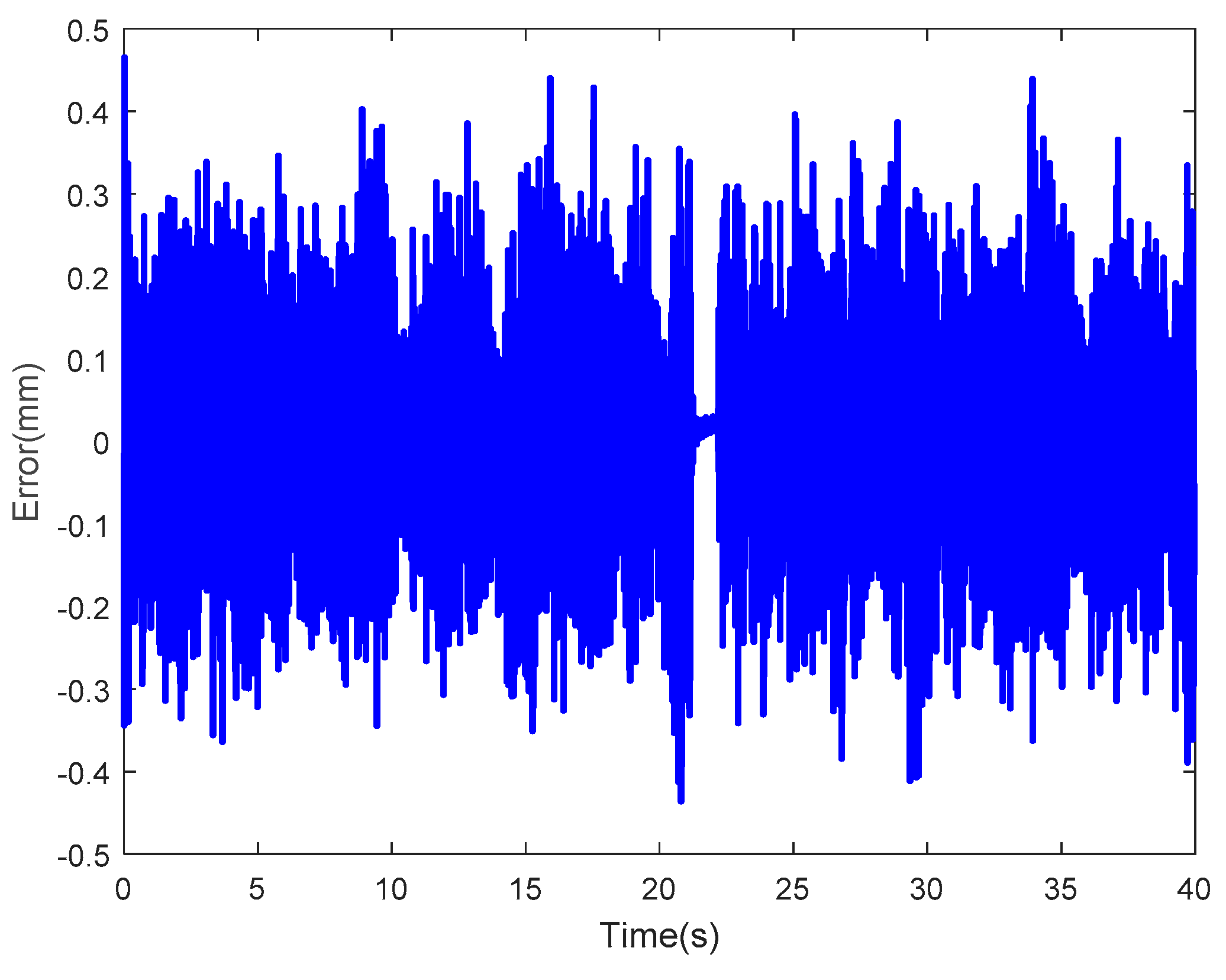
3.3. Results of the LSSVM-NARX Model

For comparison with the Prandtl-Ishlinskii model, the LSSVM-NARX model was developed, using tip displacements at a sinusoidal actuating voltage with an amplitude of 3V and a frequency of 1/2π Hz as the training data. The model parameters were $C=998.0867$ and $\sigma =0.2$. Then, the LSSVM-NARX model was verified using tip displacements at sinusoidal actuating voltages, whereby one voltage has an amplitude of 2V and a frequency of 1/2π Hz and another voltage has an amplitude of 3V and a frequency 5/2π Hz. The results (16 periods) are shown in Figure 22 and Figure 23, where the blue solid line and the red dotted line represent the tip displacements obtained experimentally and by the LSSVM-NARX model, respectively. The two curves have consistent trends despite slight differences in certain sections. Figure 24 and Figure 25 show the corresponding error curves. The errors of the LSSVM-NARX model were concentrated and most of them had absolute values below 1, although the maximum absolute value exceeded 2.5. The RMSEswere0.5147 and 0.3042, which was lower than those of the Prandtl-Ishlinskii model (0.5685 and 0.8345). In summary, the proposed LSSVM-NARX model can accurately reflect the input and output features of the IPMC actuator. Furthermore, it exhibits advantages in terms of the number of model parameters to be recognized and the recognition complexity. In addition, it has negligible requirements in terms of the form of the input data. Therefore, the model of the Pt-electrode IPMC in water was established using the LSSVM-NARX model in this study.

To verify the adaptability of LSSVM-NARX model, two random sinusoidal actuating voltages were applied, the results of experiments are shown in Figure 26 and Figure 27, the corresponding error curves of LSSVM-NARX model are shown in Figure 28 (RMSE = 0.6695) and Figure 29 (RMSE = 0.9606).

As observed form RMSEs in Figure 24, Figure 25, Figure 26 and Figure 29, although LSSVM-NARX model is superior to the Prandtl-Ishlinskii model when the inputs are tip displacements at sinusoidal actuating voltages, the RMSEs of LSSVM-NARX model are larger than those of the Prandtl-Ishlinskii model when the inputs are tip displacements at random sinusoidal actuating voltages. That is because that LSSVM-NARX model was trained using sinusoidal signals and the parameters model were not optimized, so the adaptability of the model was poor.

3.4. LSSVM-NARX Model Optimization Based on Artificial Colony Algorithm

As mentioned above, the LSSVM-NARX model has negligible requirements in terms of the form of the input data. Therefore, it was trained using the tip displacements of the IPMC actuator driven by a random sinusoidal voltage to enhance its accuracy. Figure 30a shows the random sinusoidal actuating voltage curve of this training data group, and Figure 30b shows the tip displacement curve of the IPMC actuator in response to this training data group. Owing to the direct effects of the hyper parameters ($C$ and $\sigma$) of the LSSVM-NARX model on its accuracy, the two hyperparameters were optimized using the artificial bee colony algorithm to further improve the model accuracy.

The artificial bee colony algorithm is a global optimization algorithm developed on the basis of the working principle of the bee colony. By appropriate division of labor, bees can share information about nectar sources so that the optimal nectar sources can be identified in a short time [56,57]. Optimization of the LSSVM-NARX model by the artificial bee colony algorithm can be divided into six steps:

I. Initialization of bee colony: 100 bees (employed bees and scout bees) corresponding to 100nectar sources are initialized, and the corresponding solution of each nectar source has two dimensions.

II. Search for new nectar source by bee colony: The employed bee corresponding to the ith nectar source searches for a new nectar source (i.e., new solution) according to the following equation:

$${x^{\prime }}_{id}=x_{id}+{\varphi }_{id}(x_{id}-x_{kd})$$

(16)

where i = 1, 2, …, 100, d = 1,2, ${\varphi }_{id}$ is a random number, and i ≠ k is within [–1,1].

The new nectar source identified is ${X^{\prime }}_i=\left\{{x^{\prime }}_{i1},{x^{\prime }}_{i2}\right\}$.

III. Update of nectar source: The new nectar source (${X^{\prime }}_i$) is compared with the initial one ($X_i$), and the nectar source is updated according to the following equation:

$$pi=\frac{fi{t}_i}{{\displaystyle \sum _{j=1}^{2}fi{t}_j}}$$

(17)

where $fi{t}_i$ is the fitness of $X_i$.

IV. Departure of scout bee: The employed bee corresponding to the abandoned nectar source in Step III becomes a scout bee to search for a new nectar source according to the following equation:

$$x_{id}=x_d^{\min }+r_1(x_d^{\max }-x_d^{\min })$$

(18)

where $r_1\in [0,1]$ and $x_d^{\min }$ and $x_d^{\max }$ are the upper and lower limits of the solution, respectively.

V. Memorization of the optimized nectar source: The position of the optimized nectar source (i.e., the optimized solution) is memorized, and Steps II-V are repeated 100 times.

VI. Termination of nectar source search: If a nectar source with expected fitness was identified or 100 cycles are completed, optimization is terminated and the optimized solution is generated.

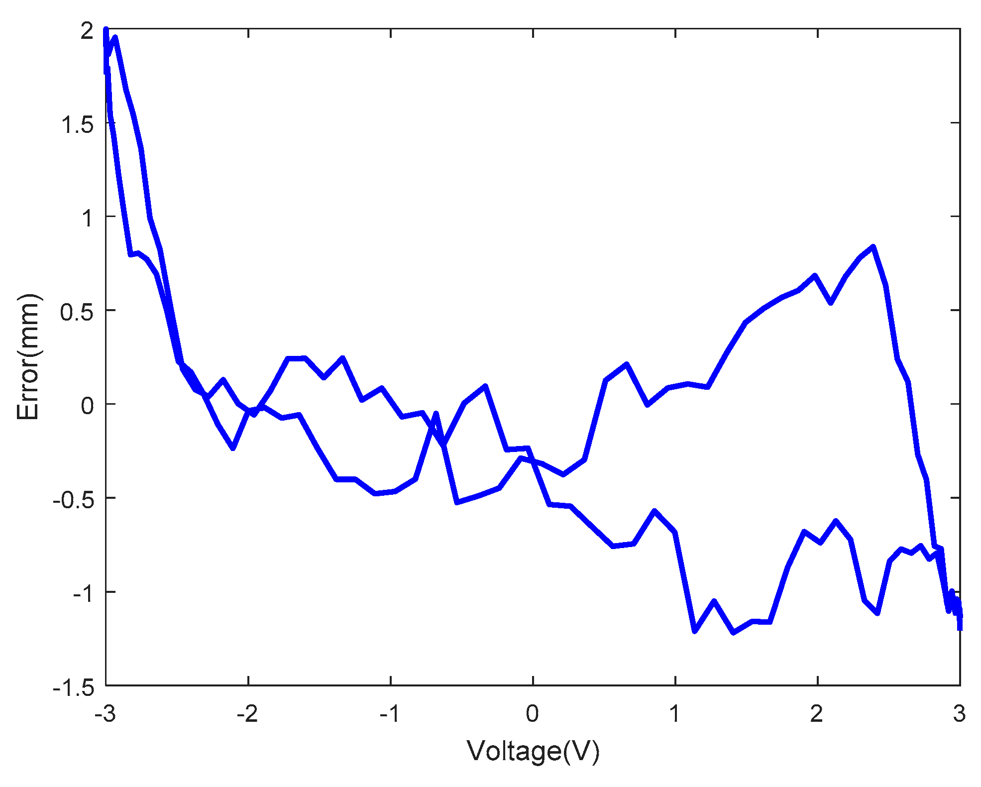
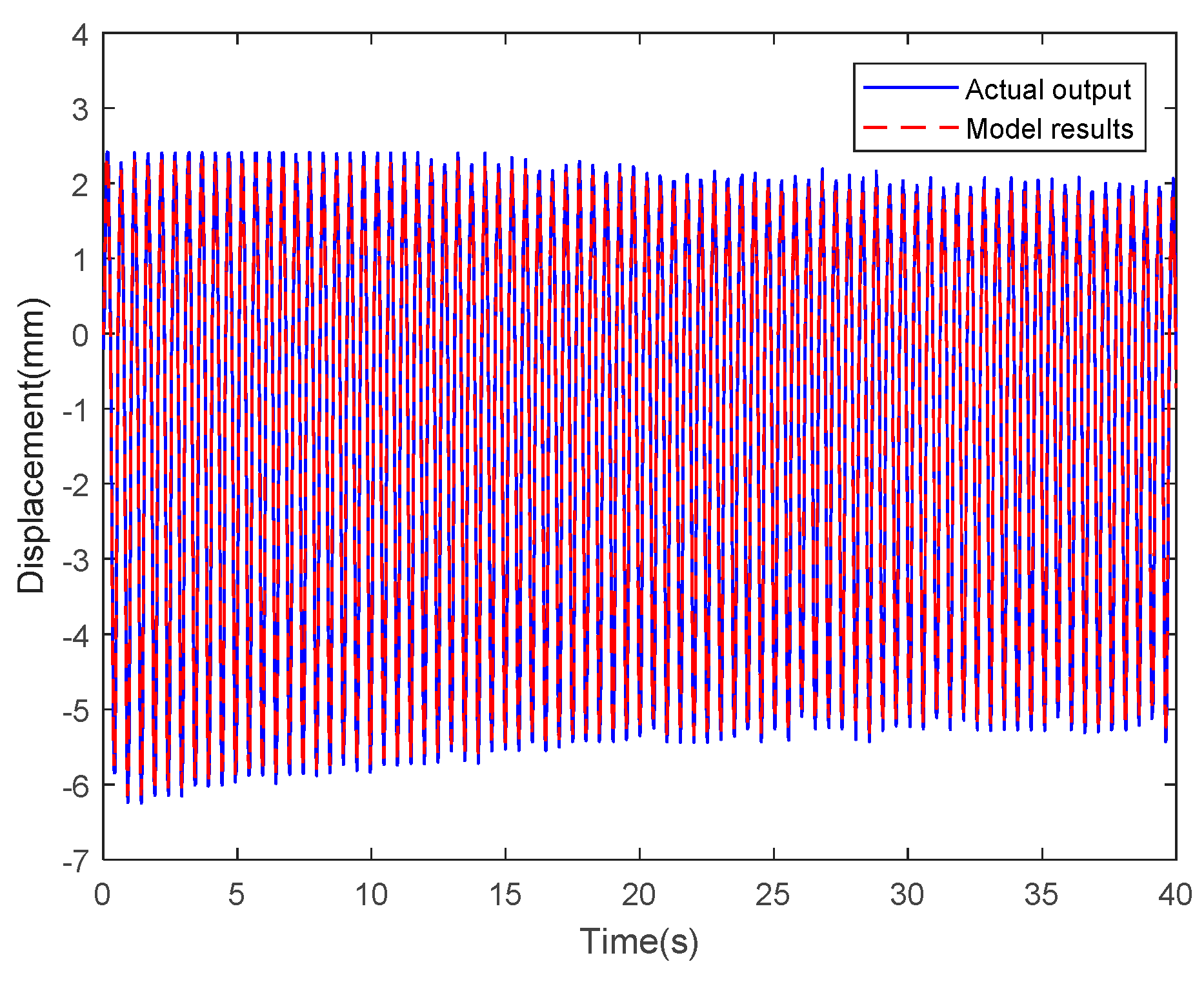
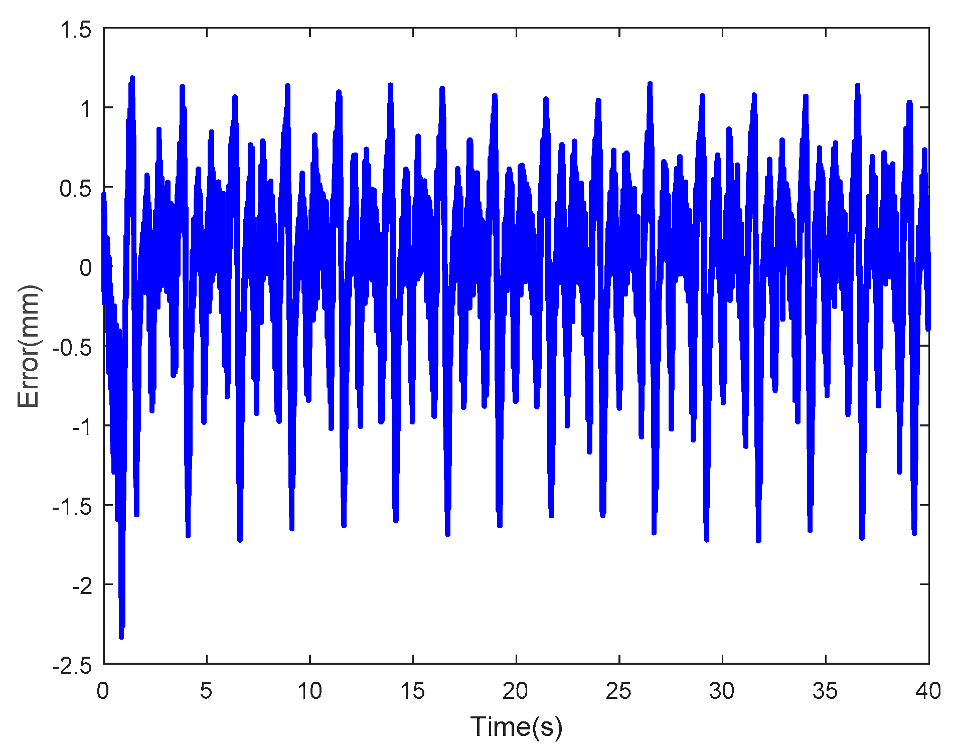
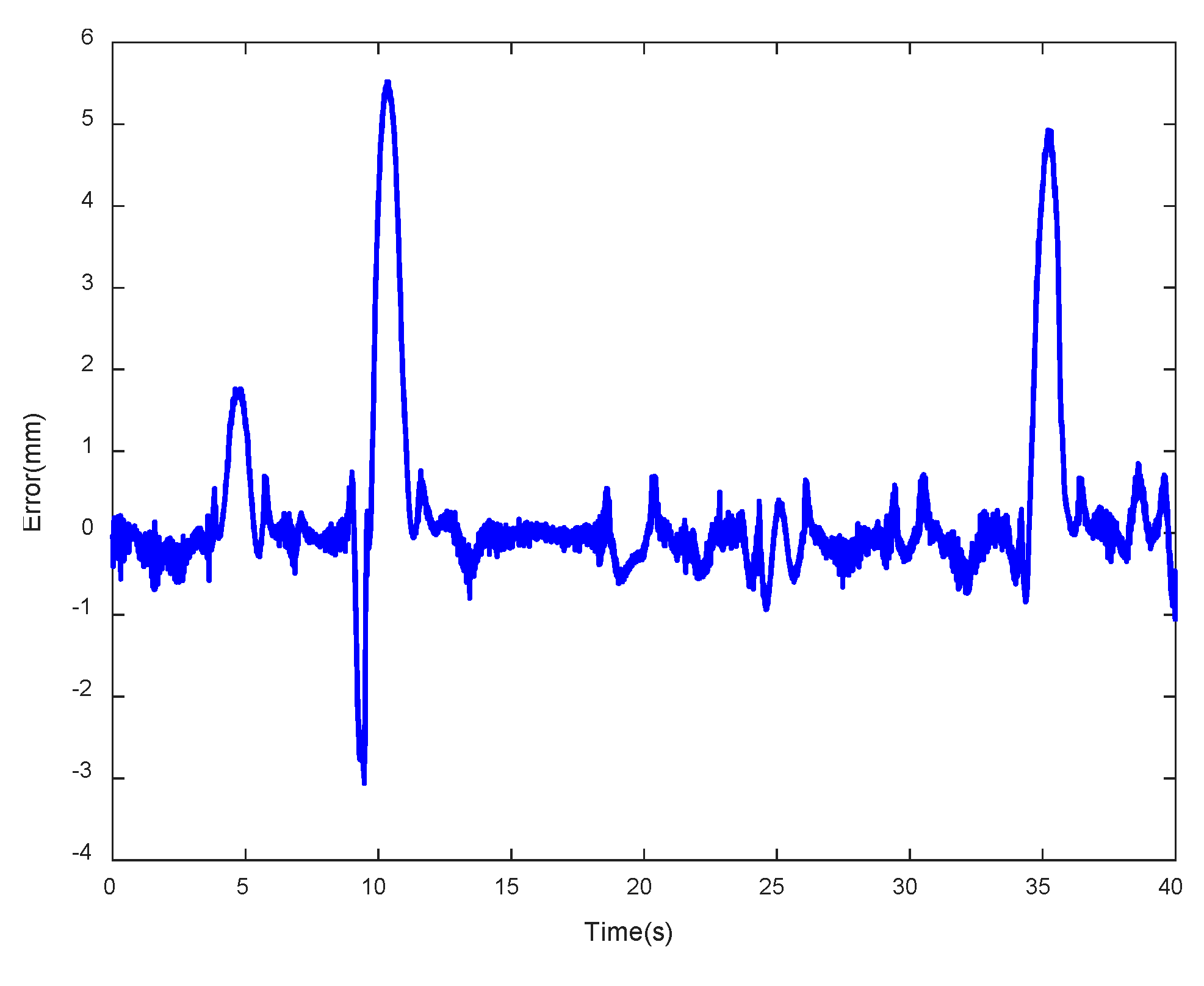
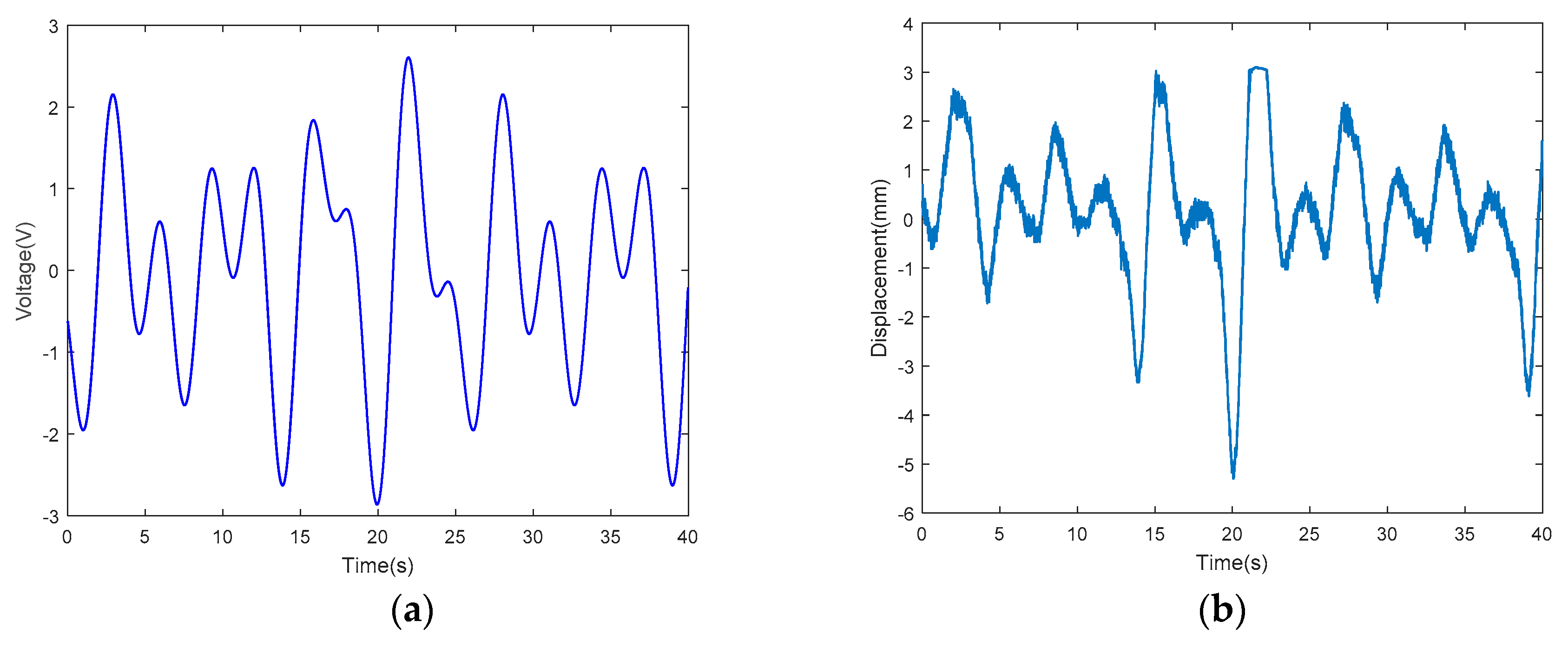
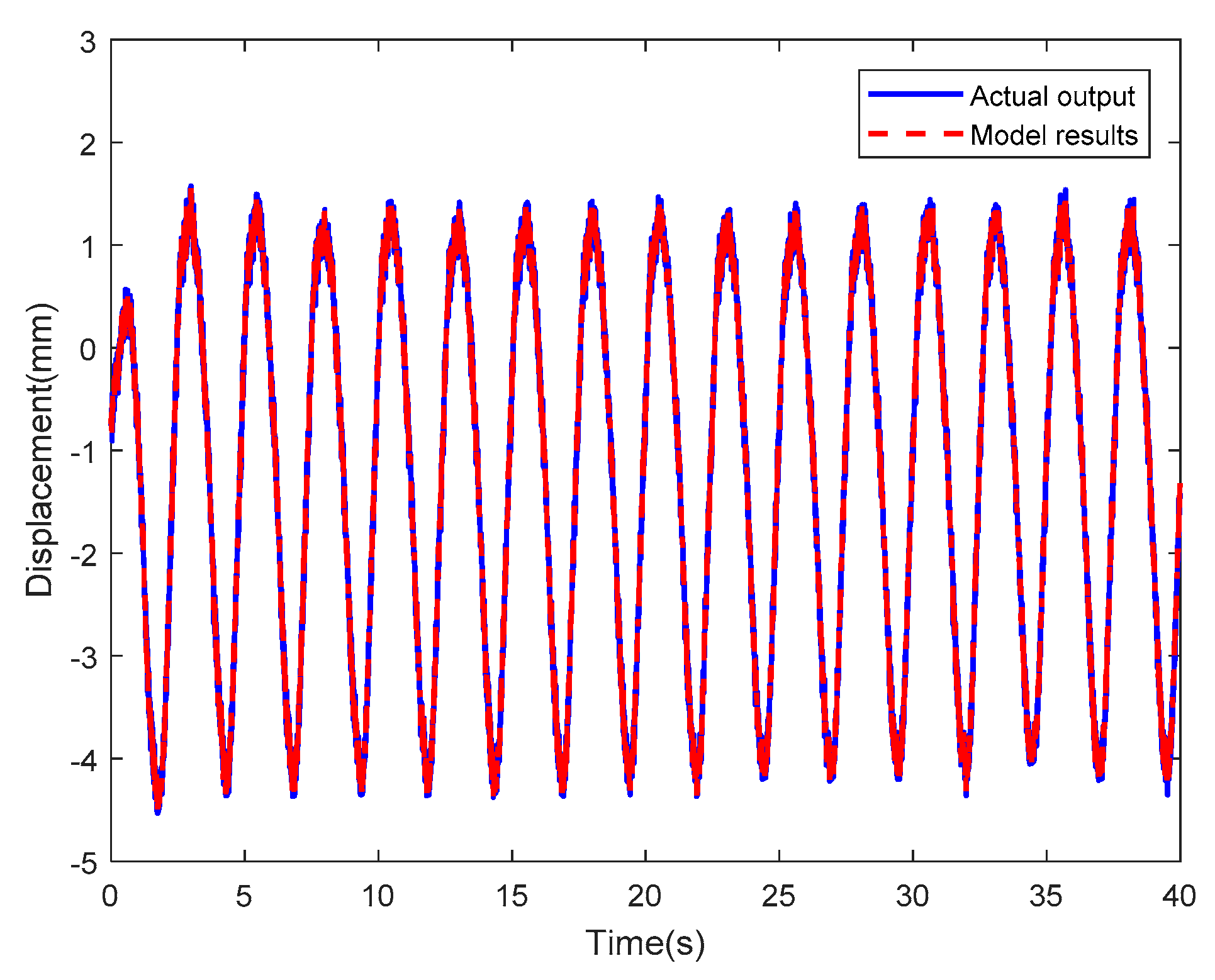
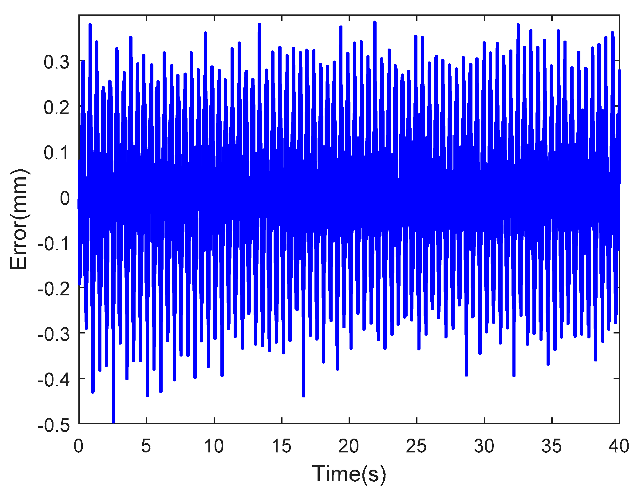
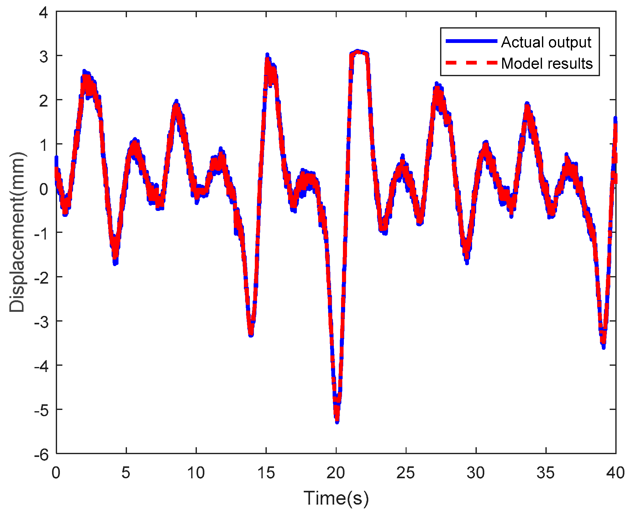
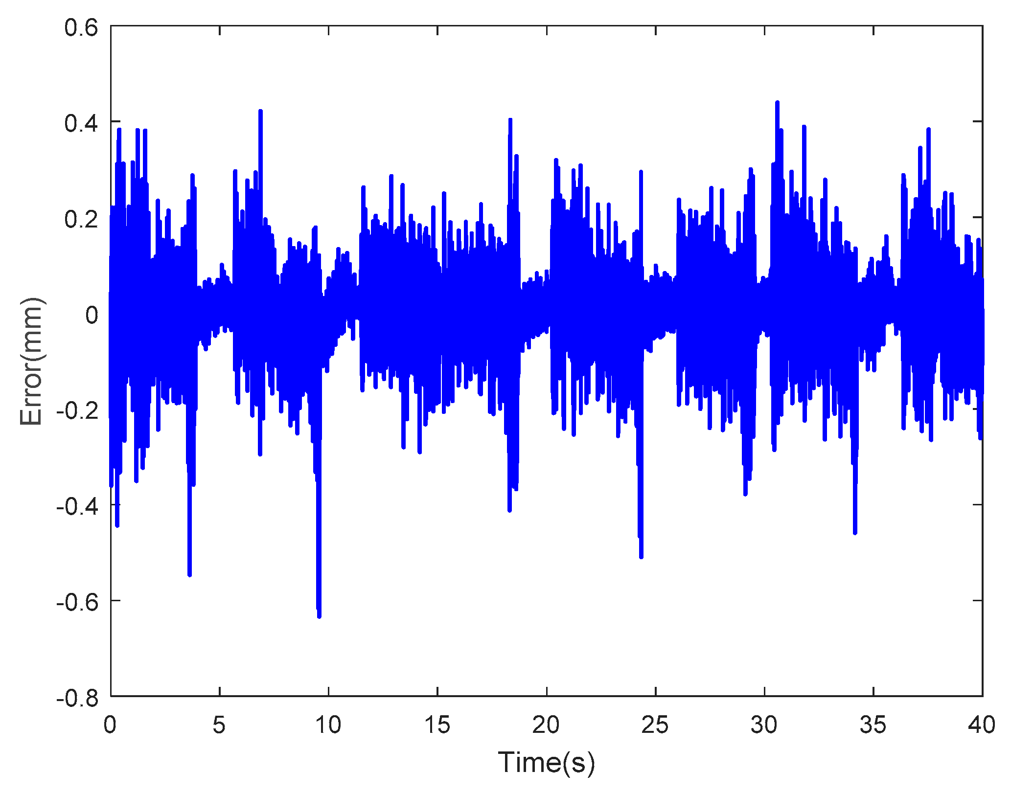
3.5. Verification of Optimized LSSVM-NARX Model

The two hyperparameters obtained by the artificial bee colony algorithm were $C_{best}=6.45\times {10}^{10}$ and ${\sigma }_{best}=7.2951\times {10}^{11}$. Then, the optimized model was verified using another data group of the IPMC driven by a random sinusoidal voltage. Figure 31 shows the random sinusoidal actuating voltage and the tip displacement of the IPMC actuator corresponding to this data group, respectively.

Figure 32; Figure 33 are the results of the optimized LSSVM-NARX model at sinusoidal actuating voltages of which one voltage is an amplitude of 2 V and a frequency of 1/2π Hz and another voltage is an amplitude of 3 V and a frequency 5/2π Hz, where the blue solid line and the red dotted line represent the tip displacements of the IPMC actuator obtained experimentally and by the optimized LSSVM-NARX model, respectively. Figure 34; Figure 35 show the corresponding error curves, of which the RMSEs are 0.1308 and 0.1261. Figure 36; Figure 37 show the results obtained by the optimized LSSVM-NARX model at random sinusoidal actuating voltages, where the blue solid line and the red dotted line represent the tip displacements of the IPMC actuator obtained experimentally and by the optimized LSSVM-NARX model, respectively. Figure 38; Figure 39 show the corresponding error curves, which have RMSEs of0.1169 and 0.0941, respectively.

As observed, whether the input signal of the optimized LSSVM-NARX model was a sinusoidal signal with different frequency and amplitude or a random sinusoidal signal, the curves are highly consistent, and the errors were smaller than the unoptimized LSSVM-NARX and the absolute values of most of the errors were below 0.4, and the RMSEs were basically around 0.1. In summary, the optimized LSSVM-NARX model is exposed to small errors and it can effectively enhance the accuracy of IPMC modeling, which has better adaptability for different types of input signals.

4. Design of IPMC Actuator Control Method Based on Inverse Controller

Strong hysteresis characteristics have adverse effects on the control accuracy of IPMC actuators. The best solution to this problem is compensation of the hysteresis characteristics by an inverse controller to reduce the control difficulty. Therefore, an inverse controller was proposed on the basis of the structural characteristics of the LSSVM-NARX model, in addition to the establishment of an accurate mathematical model by the LSSVM-NARX method. The inverse controller was combined with PID feedback control to improve the IPMC control accuracy.

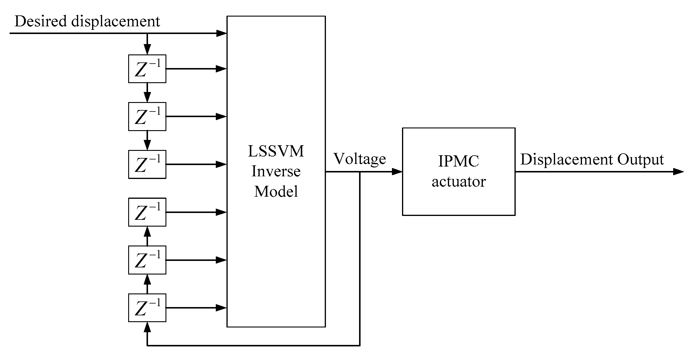
4.1. Inverse Controller Based on the LSSVM-NARX Model

Based on the LSSVM-NARX modeling discussed in Section 3, an inverse LSSVM-NARX model for inverse control was established. The input and output of the LSSVM-NARX model were the actuating voltage and IPMC displacement, respectively. The input and output of the inverse LSSVM-NARX model were the IPMC displacement and actuating voltage, respectively. Hence, the inverse LSSVM-NARX model is

$$u_l=h_1(x)={\displaystyle \sum _{l=1}^N{\alpha }_{l}K(x,x_l)}+b_1$$

(19)

where $x_l=\left[y_l,\dots y_{l-n},u_{l-1},\dots ,u_{l-m}\right]$, y_l and u_l are the input displacement and output voltage at moment l, respectively, and $h_1(x)={\omega }_1{}^{\mathrm{T}}{\phi }_1(x)+b_1$, the input space is mapped to a high-dimensional space by the nonlinear function ${\phi }_1(x)$. Furthermore, ${\omega }_1$ and $b_1$ are the weight vector and error, while $K(\cdot )$ denotes the kernel function in Equation (13).

The inverse model was established using the artificial bee colony algorithm, and $C_{in}$ and ${\sigma }_{in}$ of the inverse LSSVM-NARX model were calculated as4.0521×10⁶ and 7.1077×10³, respectively. Figure 40 shows the structure of the LSSVM-NARX inverse controller. In this inverse controller, the input and output of the inverse LSSVM-NARX model are the expected displacement and actuating voltage, respectively. Three delays were involved in both input and output. The output voltage of the inverse model was regarded as the actuating voltage of the IPMC so that the expected displacement could easily be reached by compensation.

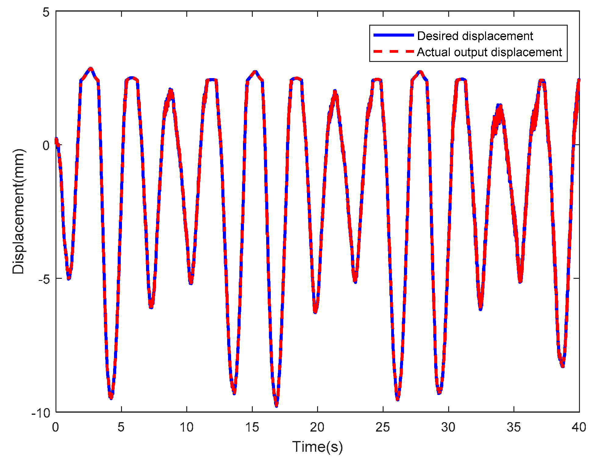
4.2. Simulation of Inverse Controller

The tip displacements of the IPMC actuator driven by a random sinusoidal voltage were regarded as the input of the LSSVM-NARX inverse controller, and the inverse controller was verified by MATLAB simulations (see Figure 41). Here, the blue solid line and the red dotted line represent the input of the inverse controller (i.e., expected tip displacement of the IPMC) and the actual tip displacement of the IPMC with the inverse controller, respectively. As observed, these two curves are highly consistent. Figure 42 shows the corresponding error curves. As observed, the control errors of the inverse controller based on the LSSVM-NARX model were small, and the absolute values of most errors were below 0.5. The root mean square error was calculated as 0.1152, indicating that the proposed inverse controller can effectively compensate the hysteresis of IPMC actuators.

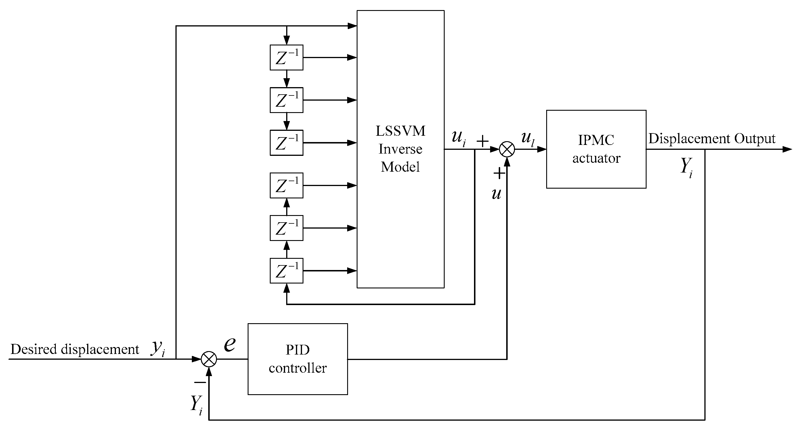
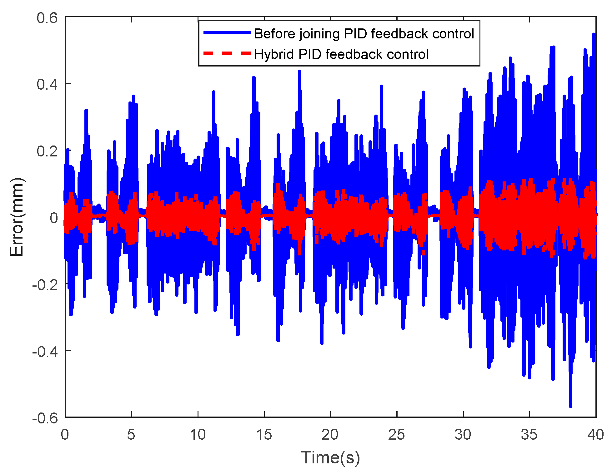
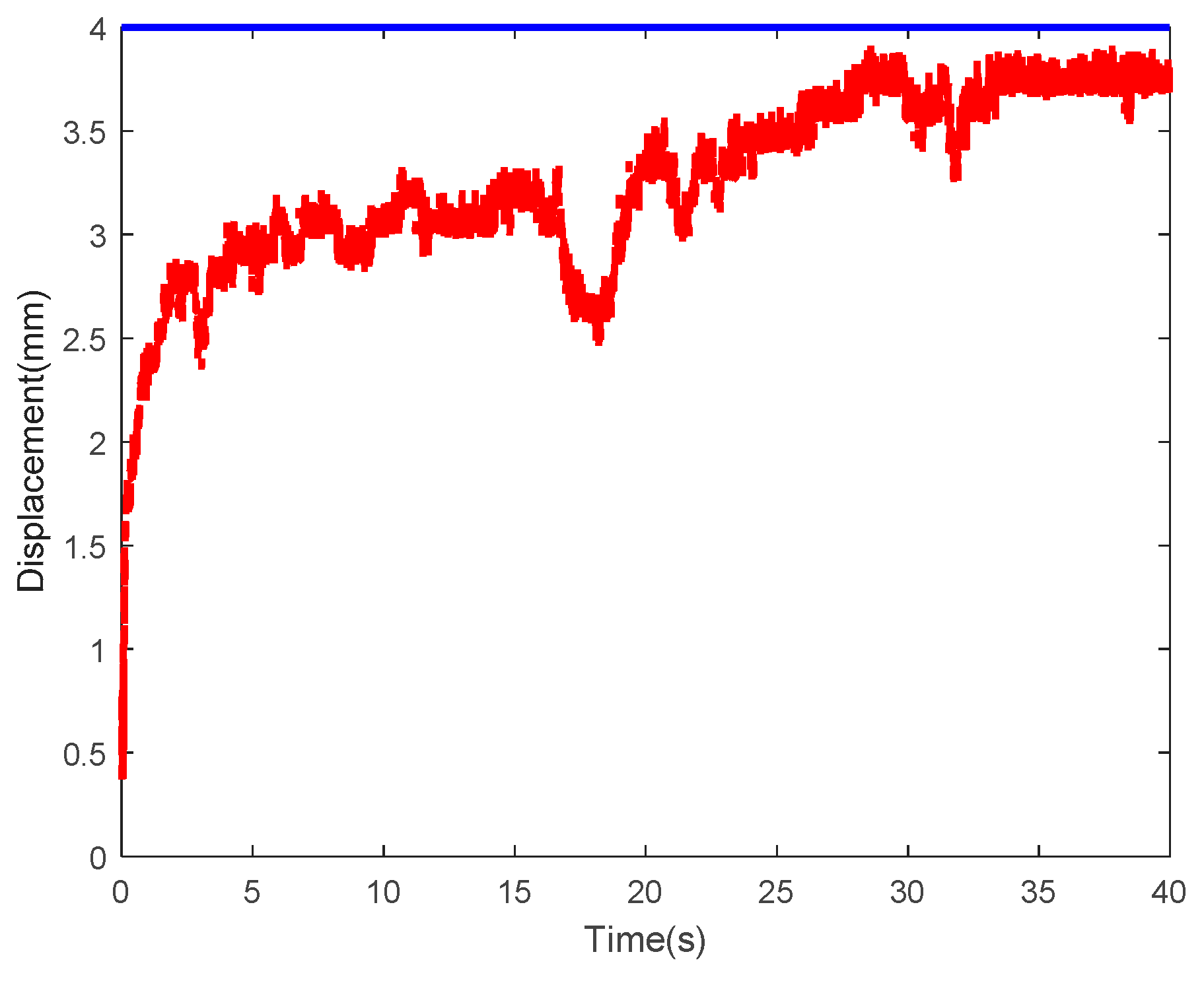
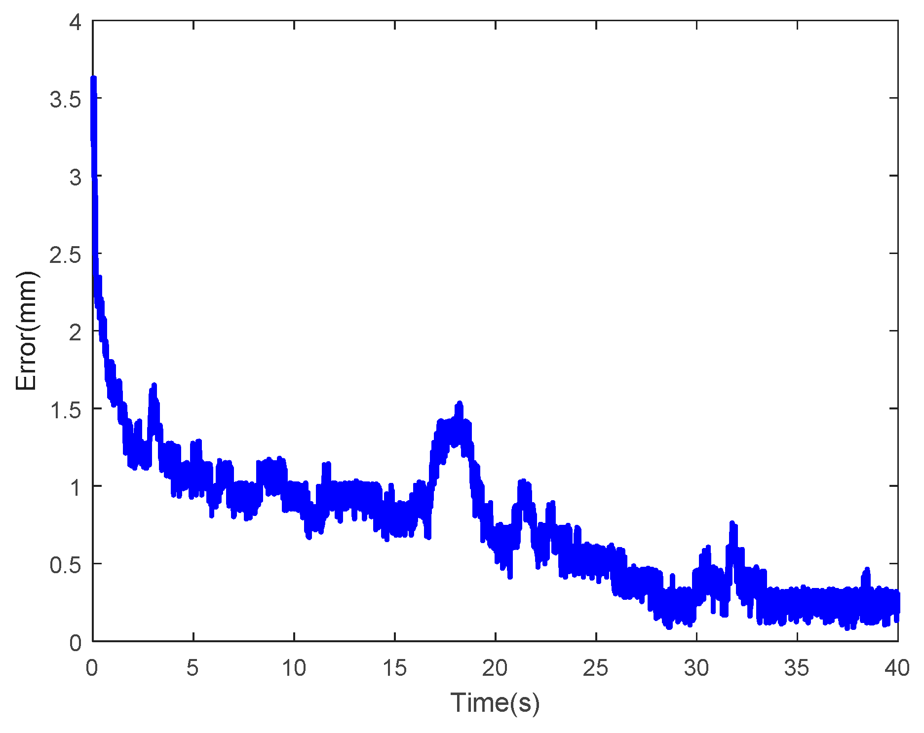
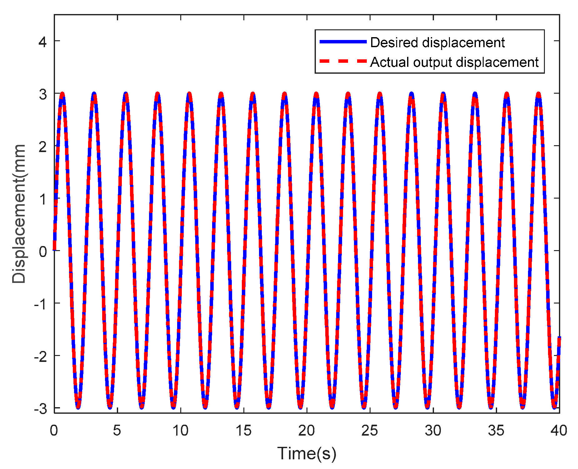
4.3. Design of Hybrid PID Control System

Although the proposed LSSVM-NARX inverse controller facilitates advances in IPMC control, it is an open-loop controller and it cannot achieve error correction. Furthermore, systems with the proposed LSSVM-NARX inverse controller exhibit poor stability and disturbance suppression. To enhance the stability and accuracy of control systems, we designed a hybrid PID controller by combining the LSSVM-NARX inverse controller with PID feedback control.

Here, $y_i$ and $u_i$ are the input displacement and output voltage of the inverse controller based on the LSSVM-NARX model at moment i, respectively. The error signal of the hybrid controller is

$$e=y_i-Y_i$$

(20)

where $Y_i$ is the output of the hybrid controller at moment i.

The output (u) of the PID controller can be calculated as

$$u=K\left(e+\frac{1}{T_I}{\displaystyle \underset{0}{\overset{l}{\int }}edl+T_D\frac{de}{dl}}\right)$$

(21)

where $K$ is the proportional gain, $T_I$ is the integration time, and $T_D$ is the differentiation time. The input ($u_l$) of the IPMC is

$$u_l=u+u_i$$

(22)

Figure 43 shows the structure of the proposed hybrid PID feedback controller. The input and output were the expected tip displacement of the IPMC ($y_i$) and actual output ($Y_i$), respectively. Essentially, the inverse LSSVM-NARX model of the actuator acts as the feedforward element of the PID feedback control, and they constitute the hybrid PID controller.

The control system was simulated using MATLAB with the following parameters: $K=1.2$, $T_I=0.87$, and $T_D=0.13$.

Figure 44 shows the control results of the hybrid PID feedback controller, where the blue solid line and the red dotted line represent the input data of the hybrid controller (i.e., expected tip displacement of IPMC) and the actual tip displacement of the IPMC actuator involving the inverse controller, respectively. As observed, these two curves are highly consistent. Figure 45 compares the output errors of the inverse controller (blue solid line) and the hybrid PID feedback controller (red dotted line). As observed, the red curve is lower than the blue one. The root means square errors of the red dotted line and the blue solid line were 0.0244 and 0.1152, respectively.

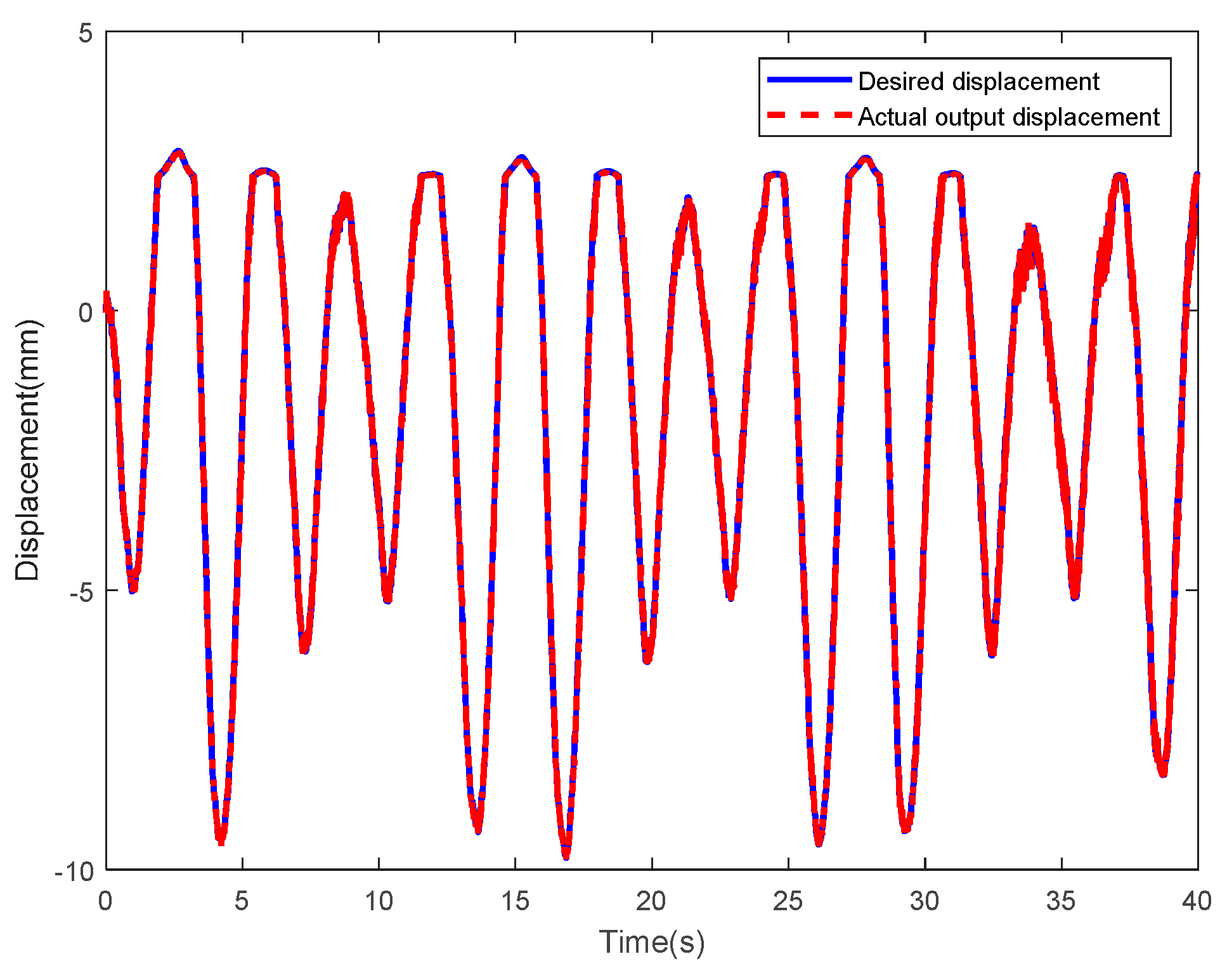
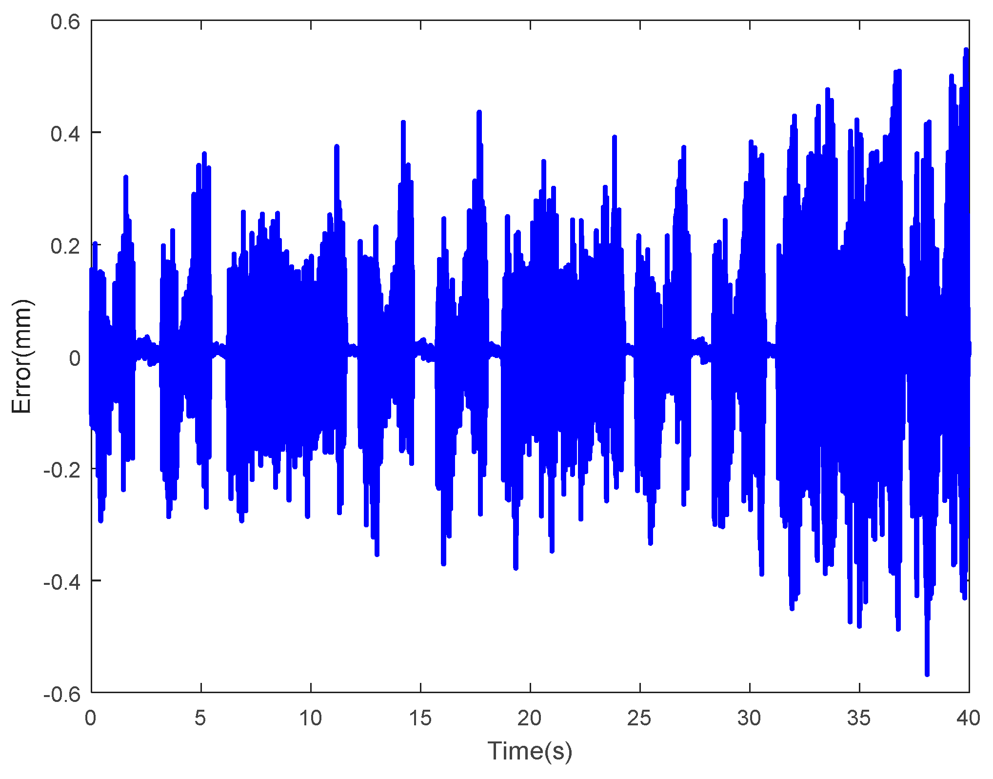
4.4. Experimental Results and Analysis

The hybrid PID feedback control was applied to the IPMC on the customized IPMC platform described above. The displacement data in different forms were used as input, regressively processed by the upper computer, and then transmitted to the inverse controller to obtain the compensating voltage of the IPMC actuator. Information about the compensating voltage and the input displacement were transmitted to the controller by serial communication. The hybrid PID feedback control system was developed by combining the inverse controller with the PID feedback control function and compensating the voltage to achieve control of the tip displacement of the IPMC actuator. Meanwhile, information about the actual tip displacements was transmitted to the upper computer by serial communication.

Figure 46 shows the control results with a constant displacement of 4mm as input, where the blue solid line and the red dotted line represent the expected displacement and actual output of the IPMC. As observed, these two curves are significantly different. Figure 47 shows the corresponding error curves. The root mean square error was calculated as 0.8756. In summary, the performances of control systems were relatively poor with constant displacement as input.

Figure 48 shows the control results with sinusoidal displacements having a frequency of 1/2π Hz and an amplitude of 2.5mm as input. Here, the blue solid line and the red dotted line represent the input and the actual output tip displacement of the IPMC, respectively. As observed, these two curves are highly consistent. Figure 49 shows the corresponding error curves. As observed, the absolute values of most errors were below 0.15. The RMSE was calculated as 0.0365. In summary, the performances of the control systems were good with regular sinusoidal displacement as input.

Figure 50 shows the control results with random sinusoidal displacement as input. Here, the blue solid line and the red dotted line represent the input and actual output tip displacement of the IPMC, respectively. As observed, these two curves are highly consistent. Figure 51 shows the corresponding error curves. As observed, the absolute values of most errors were below 0.08. The root mean square error was calculated as0.0306. In summary, the performances of control systems were also good with random sinusoidal displacement as input.

Figure 52 shows the spectrum of the input random sinusoidal displacement of the control system shown in Figure 50. As observed, the frequency and amplitude of input random sinusoidal displacement were 0–0.7 Hz and −9–4 mm, respectively. Hence, the feasibility of the hybrid PID feedback control can be effectively verified with random sinusoidal displacement as input.

The control system exhibited poor performance and severe errors with constant input displacement. The LSSVM-NARX inverse controller in the hybrid PID feedback controller was developed on the basis of the hysteresis characteristics of the IPMC actuators, which are dynamically nonlinear, especially in the case of input voltages with varying amplitude and frequency. However, at constant input displacement, the IPMC nonlinearity is mainly reflected as creep characteristics, resulting in limited accuracy of the control system. With regular or random sinusoidal displacements as input, the control system exhibited good performance and small control errors. Therefore, our experiments demonstrated that the proposed control system could effectively overcome IPMC hysteresis and achieve good control effects.

5. Conclusions and Prospects

As an electrically driven intelligent composite, an IPMC used as an actuator exhibits strong hysteresis characteristics, resulting in limited control accuracy. This study aimed to develop a control approach that can reduce, if not eliminate, the adverse effects of hysteresis characteristics on IPMC control. First, the performance of an electrically driven Pt-electrode IPMC was tested. Specifically, the tip displacements of the IPMC at different voltages were measured and the hysteresis characteristics of the IPMC actuator were analyzed. To overcome the IPMC hysteresis, the tip displacements of an electrically driven IPMC actuator were modeled using the LSSVM-NARX model and an artificial bee colony algorithm was proposed to optimize the parameters of the LSSVM-NARX model, and compared with those obtained using the conventional Prandtl-Ishlinskii model. The results indicated that the RMSEs of optimized LSSVM-NARX model was only about 0.1, which is far less than that of the Prandtl-Ishlinskii model (0.6–0.8); therefore, modeling of the Pt-electrode IPMC in water by the LSSVM-NARX model is accurate and efficient. Subsequently, an LSSVM-NARX inverse controller was designed to compensate the hysteresis characteristics of the IPMC, and it was combined with PID feedback control to generate a hybrid PID feedback controller that is capable of accurate control of the Pt-electrode IPMC in water. The experiments indicated that the hybrid PID feedback controller can control the precise trajectory of tip displacement of IPMC with the RMSE of about 0.03 in the range of 0 to 0.7 Hz. Those studies demonstrated the feasibility and effectiveness of the proposed control approach.

In addition, if the purity of the distilled water soaked by IPMC is maintained and the electrode voltage of IPMC is less than 3V, the service life of the IPMC can reach 2600–2800 h, during which time the models and control methods in article are applicable. Meanwhile, the IPMC was exposed to severe creep if the expected displacement remained constant and the continuous control time exceeded 4h. Therefore, the ways to improve service life of IPMC and compensation of creep for continuous control of IPMC over a long time should be investigated for further improvement.

References

1. Wang, H. Application of intelligent materials in the control system. J. Comput. Theor. Nanosci. 2015, 12, 2830–2836. [Google Scholar] [CrossRef]
2. Mutlu, R.; Alici, G.; Xiang, X.; Li, W. Electro-mechanical modelling and identification of electroactive polymer actuators as smart robotic manipulators. Mechatronics 2014, 24, 241–251. [Google Scholar] [CrossRef] [Green Version]
3. Hong, W.Y.J.; Almomani, A.; Cchen, Y.F.; Jamshidi, R.; Montazami, R. Soft ionic electroactive polymer actuators with tunable non-linear angular deformation. Materials 2017, 10, 664. [Google Scholar] [CrossRef] [PubMed]
4. Guo, J.; Bamber, T.; Zhao, Y.; Chamberlain, M.R.; Justham, L.; Jackson, M. Toward adaptive and intelligent electro-adhesives for robotic material handling. IEEE Robot. Autom. Lett. 2017, 2, 538–545. [Google Scholar] [CrossRef]
5. Alekseev, N.I.; Broiko, A.P.; Kalenov, V.E. Structure of a graphene-modified electroactive polymer for membranes of biomimetic systems: Simulation and experiment. J. Struct. Chem. 2018, 59, 1707–1718. [Google Scholar] [CrossRef]
6. Bashir, M.; Rajendran, P. A review on electroactive polymers development for aerospace applications. J. Intell. Mater. Syst. Struct. 2018, 28, 3681–3695. [Google Scholar] [CrossRef]
7. Chang, L.F.; Liu, Y.F.; Yang, Q.; Yu, L.; Liu, J.; Zhu, Z.; Lu, P.; Wu, Y.; Hu, Y. Ionic electroactive polymers used in bionic robots: A review. J. BionicEng. 2018, 15, 765–782. [Google Scholar] [CrossRef]
8. Palza, H.; Zapata, P.A.; Angulo-Pineda, C. Electroactive smart polymers for biomedical applications. Materials 2019, 12, 277. [Google Scholar] [CrossRef]
9. Chidsey, C.E.; Murray, R.W. Electroactive polymers and macromolecular electronics. Science 1986, 231, 25–31. [Google Scholar] [CrossRef]
10. Tiwari, R.; Garcia, E. The state of understanding of ionic polymer metal composite architecture: A review. SmartMater. Struct. 2011, 20. [Google Scholar] [CrossRef]
11. Li, H.Y.; Liu, Y.L. Nafion-functionalized electrospun poly (vinylidene fluoride) (PVDF) nanofibers for high performance proton exchange membranes in fuel cells. J. Mater. Chem. A 2014, 2, 3783–3793. [Google Scholar] [CrossRef]
12. Peng, K.J.; Lai, J.Y.; Liu, Y.L. Nanohybrids of graphene oxide chemically-bonded with Nafion: Preparation and application for proton exchange membrane fuel cells. J. Membr. Sci. 2016, 514, 86–94. [Google Scholar] [CrossRef]
13. Kim, D.J.; Jo, M.J.; Nam, S.Y. A review of polymer-nanocomposite electrolyte membranes for fuel cell application. J. Ind. Eng. Chem. 2015, 21, 36–52. [Google Scholar] [CrossRef]
14. Liu, Y.; Chang, L.; Hu, Y.; Niu, Q.; Yu, L.; Wang, Y.; Lu, P.; Wu, Y. Rough interface in IPMC: Modeling and its influence analysis. SmartMater. Struct. 2018, 27. [Google Scholar] [CrossRef]
15. Shen, Q.; Stalbaum, T.; Minaian, N.; Oh, I.K.; Kim, K.J. A robotic multiple-shape-memory ionic polymer-metal composite (IPMC) actuator: Modeling approach. SmartMater. Struct. 2019, 28. [Google Scholar] [CrossRef]
16. Zhu, Z.C.; Bian, C.S.; Ru, J.; Bai, W.F.; Chen, H.L. Rapid deformation of IPMC under a high electrical pulse stimulus inspired by action potential. SmartMater. Struct. 2019, 28. [Google Scholar] [CrossRef]
17. Jain, R.K.; Datta, S.; Majumder, S. Design and control of an IPMC artificial muscle finger for micro gripper using EMG signal. Mechatronics 2013, 23, 381–394. [Google Scholar] [CrossRef]
18. Tadokoro, S.; Yamagami, S.; Takamori, T.; Oguro, K. An actuator model of ICPF for robotic applications on the basis of physicochemical hypotheses. In Proceedings of the IEEE International Conference on Robotics & Automation, San Francisco, CA, USA, 24–28 April 2000; pp. 1340–1346. [Google Scholar]
19. Tadokoro, S.; Fukuhara, M.; Maeba, Y.; Takamori, T. A dynamic model of ICPF actuator considering ion-induced lateral strain for molluskan robotics. In Proceedings of the IEEE/RSJ International Conference on Intelligent Robots & Systems, Lausanne, Switzerland, 30 September–4 October 2002. [Google Scholar]
20. Bonomo, C.; Fortuna, L.; Giannone, S.; Mazza, D. A circuit to model the electrical behavior of an ionic polymer-metal composite. IEEE Trans. Circuits Syst. I: Regul. Pap. 2012, 53, 338–350. [Google Scholar] [CrossRef]
21. Anh, H.P.H.; Ahn, K.K. Identification of pneumatic artificial muscle manipulators by a MGA-based nonlinear NARX fuzzy model. Mechatronics 2009, 19, 106–133. [Google Scholar] [CrossRef]
22. Chen, Z.; Hedgepeth, D.R.; Tan, X. A nonlinear, control-oriented model for ionic polymer-metal composite actuators. SmartMater. Struct. 2009, 18, 1851–1856. [Google Scholar] [CrossRef]
23. Nam, D.N.C.; Ahn, K.K. Identification of an ionic polymer metal composite actuator employing Preisach type fuzzy NARX model and Particle Swarm Optimization. Sens. Actuators A Phys. 2012, 183, 105–114. [Google Scholar] [CrossRef]
24. Lagosh, A.V.; Broyko, A.P.; Kalyonov, V.E.; Khmelnitskiy, I.K.; Luchinin, V.V. Modeling of IPMC actuator. In Proceedings of the 2017 IEEE Conference of Russian Young Researchers in Electrical and Electronic Engineering (EIConRus), St. Petersburg, Russia, 1–3 February 2017; pp. 916–918. [Google Scholar]
25. Zamyad, H.; Naghavi, N. Behavior identification of IPMC actuators using laguerre-MLP network with consideration of ambient temperature and humidity effects on their performance. IEEETrans. Instrum. Meas. 2018, 67, 2723–2732. [Google Scholar] [CrossRef]
26. Oh, S.J.; Kim, H. A study on the control of an IPMC actuator using an adaptive fuzzy algorithm. KSME Int. J. 2004, 18, 1–11. [Google Scholar] [CrossRef]
27. Hao, L.; Li, Z. Modeling and adaptive inverse control of hysteresis and creep in ionic polymer-metal composite actuators. SmartMater. Struct. 2010, 19, 865–870. [Google Scholar] [CrossRef]
28. Sun, Z.; Hao, L.; Chen, W.; Li, Z.; Liu, L. A novel discrete adaptive sliding modelike control method for ionic polymermetal composite manipulators. SmartMater. Struct. 2013, 22, 95–108. [Google Scholar] [CrossRef]
29. Hao, L.; Chen, Y.; Sun, Z. The sliding mode control for different shapes and dimensions of IPMC on resisting its creep characteristics. SmartMater. Struct. 2015, 24, 964–978. [Google Scholar] [CrossRef]
30. Chen, Y.; Hao, L.; Yang, H.; Gao, J. Kriging modeling and SPSA adjusting PID with KPWF compensator control of IPMC gripper for mm-sized objects. Rev. Sci. Instrum. 2017, 88, 1–9. [Google Scholar] [CrossRef]
31. Caponetto, R.; Luca, V.D.; Graziani, S. A multiphysics model of IPMC actuators dependence on relative humidity. In Proceedings of the 2015 IEEE International Instrumentation and Measurement Technology Conference (I2MTC) Proceedings, Pisa, Italy, 11–14 May 2015; pp. 1482–1487. [Google Scholar]
32. Kim, M.H.; Kim, K.Y.; Lee, J.H.; Jho, J.Y.; Kim, D.M.; Rhee, K.; Lee, S.J. An experimental study of force control of an IPMC actuated two-link manipulator using time-delay control. SmartMater. Struct. 2016, 25, 117–130. [Google Scholar] [CrossRef]
33. Khawwaf, J.; Zheng, J.; Al-Cihanimi, A.; Man, Z.; Nagarajah, R. Modeling and tracking control of an IPMC actuator for underwater applications. In Proceedings of the 2016 International Conference on Advanced Mechatronic Systems (ICAMechS), Melbourne, VIC, Australia, 30 November–3 December 2016; pp. 550–554. [Google Scholar]
34. Bernat, J.; Kolota, J. Adaptive observer-based control for an IPMC actuator under varying humidity conditions. SmartMater. Struct. 2018, 27, 55–64. [Google Scholar] [CrossRef]
35. Sainag, T.L.; Sujoy, M. Optimal position control of ionic polymer metal composite using particle swarm optimization. In Proceedings of the SPIE 20th Conference on Electroactive Polymers Actuators and Devices, Denver, CO, USA, 27 March 2018; Volume 18, pp. 1059–1068. [Google Scholar]
36. Darnag, R.; Minaoui, B.; Fakir, M. QSAR models for prediction study of HIV protease inhibitors using support vector machines, neural networks and multiple linear regression. Arabian J. Chem. 2017, 10, S600–S608. [Google Scholar] [CrossRef] [Green Version]
37. Ma, Y.; Zhang, X.; Xu, M.; Xie, S. Hybrid model based on preisach and support vector machine for novel dual-stack piezoelectric actuator. Mech. Syst. Signal Process. 2013, 34, 156–172. [Google Scholar] [CrossRef]
38. Wong, P.K.; Xu, Q.; Vong, C.M.; Wong, H.C. Rate-dependent hysteresis modeling and control of a piezostage using online support vector machine and relevance vector machine. IEEE Trans. Ind. Electron. 2012, 59, 1988–2001. [Google Scholar] [CrossRef]
39. Mao, X.; Wang, Y.; Liu, X.; Guo, Y. An adaptive weighted least square support vector regression for hysteresis in piezoelectric actuators. Sens. Actuators A Phys. 2017, 263, 423–429. [Google Scholar] [CrossRef] [Green Version]
40. Yang, J.; Bouzerdoum, A.; Phung, S. A Training algorithm for sparse LS-SVM using compressive sampling. In Proceedings of the IEEE International Conference on Acoustics, Speech, and Signal Processing, Dallas, TX, USA, 14–19 March 2010; pp. 2054–2057. [Google Scholar]
41. Napoli, R.; Piroddi, L. Nonlinear active noise control with NARX models. IEEE Trans. Audio Speech Lang. Process. 2010, 18, 286–295. [Google Scholar] [CrossRef]
42. Sahoo, H.K.; Dash, P.K.; Rath, N.P. NARX model based nonlinear dynamic system identification using low complexity neural networks and robust H filter. Appl. Soft Comput. 2013, 13, 3324–3334. [Google Scholar] [CrossRef]
43. Wang, H.; Song, G. Innovative NARX recurrent neural network model for ultra-thin shape memory allow wire. Neurocomputing 2014, 134, 289–295. [Google Scholar] [CrossRef]
44. Asgari, H. NARX models for simulation of the start-up operation of a single-shaft gas turbine. Appl. Therm. Eng. 2016, 93, 368–376. [Google Scholar] [CrossRef]
45. Mao, X.F.; Wang, Y.J.; Liu, X.D. A hybrid feedforward-feedback hysteresis compensator in piezoelectric actuators based on least-squares support vector machine. IEEE Trans. Ind. Electron. 2018, 65, 5704–5711. [Google Scholar] [CrossRef]
46. Xu, Q. Identification and compensation of piezoelectric hysteresis without modeling hysteresis inverse. IEEE Trans. Ind. Electron. 2013, 60, 3927–3937. [Google Scholar] [CrossRef]
47. Al Janaideh, M.; Rakotondrabe, M.; Aljanaidwh, O. Further Results on Hysteresis Compensation of Smart Micropositioning Systems with the Inverse Prandtl-Ishlinskii Compensator. IEEE Trans. Control Syst. Technol. 2015, 24, 428–439. [Google Scholar] [CrossRef]
48. Jiang, C.; Deng, M.; Inoue, A. A novel modeling of nonlinear plants with hysteresis described by non-symmetric play operator. In Proceedings of the 7th World Congress on Intelligent Control and Automation, Chongqing, China, 25–27 June 2008; pp. 2221–2224. [Google Scholar]
49. Guzman, S.M.; Paz, J.O.; Tagert, M.L.M.; Mercer, A.E. Evaluation of seasonally classified inputs for the prediction of daily groundwater levels: NARX networks vs support vector machines. Environ. Modeling Assess. 2019, 24, 223–234. [Google Scholar] [CrossRef]
50. Ezzeldin, R.; Hatata, A. Application of NARX neural network model for discharge prediction through lateral orifices. Alex. Eng. J. 2018, 54, 2991–2998. [Google Scholar] [CrossRef]
51. Jaleel, E.A.; Aparna, K. Identification of realistic distillation column using NARX based hybrid artificial neural network and artificial bee colony algorithm. J. Intell. Fuzzy Syst. 2018, 34, 2075–2086. [Google Scholar] [CrossRef]
52. Avellina, M.; Brankovic, A.; Piroddi, L. Distributed randomized model structure selection for NARX models. Int. J. Adapt. Control Signal Process. 2017, 31, 1853–1870. [Google Scholar] [CrossRef]
53. Suykens, J.A.K.; Vandewalle, J. Least squares support vector machine classifiers. Neural Process. Lett. 1999, 9, 293–300. [Google Scholar]
54. Kaytez, F.; Taplamacioglu, M.C.; Cam, E.; Hardalac, F. Foreacsting electricity consumption: A comparison of regression analysis, neural networks and least squares support vector machine. Int. J. Electr. Power Energy Syst. 2015, 67, 431–438. [Google Scholar] [CrossRef]
55. Cao, L.J.; Tay, F.H. Support vector machine with adaptive parameters in financial time series forcasting. IEEE Trans. Neural Netw. 2003, 14, 1506–1518. [Google Scholar] [CrossRef]
56. Karaboga, D. AnIdea Based on Honey Bee Swarm for Numerical Optimization; Technical Report; Computers Engineering Department, Engineering Faculty, Eriyes University: Kayseri, Turkey, 2005. [Google Scholar]
57. Tereshko, V.; Loengarov, A. Collective decision-making in honeybee foraging dynamics. Comput. Inf. Syst. J. 2005, 9, 1–7. [Google Scholar]
Figure 1. Structure and mechanism of electrically driven deformations of IPMC.
Mathematics 07 00741 g001
Figure 2. Customized platform for IPMC actuators.
Mathematics 07 00741 g002
Figure 3. Structure diagram of the IPMC actuator platform.
Mathematics 07 00741 g003
Figure 4. Displacement compensation diagram of IPMC actuators.
Mathematics 07 00741 g004
Figure 5. Tip displacement at actuating voltage with amplitude of 1V and frequency of 0.5/2π Hz.
Mathematics 07 00741 g005
Figure 6. Tip displacement at actuating voltage with amplitude of 1V and frequency of 1/2π Hz.
Mathematics 07 00741 g006
Figure 7. Tip displacement at actuating voltage with amplitude of 1V and frequency of 5/2π Hz.
Mathematics 07 00741 g007
Figure 8. Tip displacement at actuating voltage with amplitude of 2V and frequency of 0.5/2π Hz.
Mathematics 07 00741 g008
Figure 9. Tip displacement at actuating voltage with amplitude of 2V and frequency of 1/2π Hz.
Mathematics 07 00741 g009
Figure 10. Tip displacement at actuating voltage with amplitude of 2V and frequency of 5/2π Hz.
Mathematics 07 00741 g010
Figure 11. Tip displacement at actuating voltage with amplitude of 3V and frequency of 0.5/2π Hz.
Mathematics 07 00741 g011
Figure 12. Tip displacement at actuating voltage with amplitude of 3V and frequency of 1/2π Hz.
Mathematics 07 00741 g012
Figure 13. Tip displacement at actuating voltage with amplitude of 3V and frequency of 5/2π Hz.
Mathematics 07 00741 g013
Figure 14. Schematic diagram of play hysteresis operator.
Mathematics 07 00741 g014
Figure 15. Structure of the proposed Prandtl-Ishlinskii model.
Mathematics 07 00741 g015
Figure 16. Results of the Prandtl-Ishlinskii model at sinusoidal actuating voltage with amplitude of 2V and frequency of 1/2π Hz.
Mathematics 07 00741 g016
Figure 17. Results of the Prandtl-Ishlinskii model at sinusoidal actuating voltage with amplitude of 3V and frequency of 5/2π Hz.
Mathematics 07 00741 g017
Figure 18. Errorof the Prandtl-Ishlinskii model at sinusoidal actuating voltage with amplitude of 2V and frequency of 1/2π Hz (RMSE = 0.5685).
Mathematics 07 00741 g018
Figure 19. Error of the Prandtl-Ishlinskii model at sinusoidal actuating voltage with amplitude of 3V and frequency of 5/2π Hz (RMSE = 0.8345).
Mathematics 07 00741 g019
Figure 20. Structure of NARX.
Mathematics 07 00741 g020
Figure 21. Structure of the LSSVM-NARX model.
Mathematics 07 00741 g021
Figure 22. Results of the LSSVM-NARX model at sinusoidal actuating voltage with amplitude of 2V and frequency of 1/2π Hz.
Mathematics 07 00741 g022
Figure 23. Results of the LSSVM-NARX model at sinusoidal actuating voltage with amplitude of 3V and frequency of 5/2π Hz.
Mathematics 07 00741 g023
Figure 24. Error of the LSSVM-NARX model at sinusoidal actuating voltage with amplitude of 2V and frequency of 1/2π Hz (RMSE = 0.5147).
Mathematics 07 00741 g024
Figure 25. Error of the LSSVM-NARX model at sinusoidal actuating voltage with amplitude of 3V and frequency of 5/2π Hz (RMSE = 0.3042).
Mathematics 07 00741 g025
Figure 26. Results of the LSSVM-NARX model at random sinusoidal actuating voltage I.
Mathematics 07 00741 g026
Figure 27. Results of the LSSVM-NARX model at random sinusoidal actuating voltage II.
Mathematics 07 00741 g027
Figure 28. Error of the LSSVM-NARX model at random sinusoidal actuating voltage I (RMSE = 0.6695).
Mathematics 07 00741 g028
Figure 29. Error of the LSSVM-NARX model at random sinusoidal actuating voltage II (RMSE = 0.9606).
Mathematics 07 00741 g029
Figure 30. The displacement of the tip by the Random sinusoidal drive voltage I: (a) Random sinusoidal drive voltage I; (b) Random sinusoidal tip displacement I.
Mathematics 07 00741 g030
Figure 31. The displacement of tip by the Random sinusoidal drive voltage II: (a) Random sinusoidal drive voltage II; (b) Random sinusoidal tip displacement II.
Mathematics 07 00741 g031
Figure 32. Results of the optimized LSSVM-NARX model at sinusoidal actuating voltage with amplitude of 2V and frequency of 1/2π Hz.
Mathematics 07 00741 g032
Figure 33. Results of the optimized LSSVM-NARX model at sinusoidal actuating voltage with amplitude of 3V and frequency of 5/2π Hz.
Mathematics 07 00741 g033
Figure 34. Error of the optimized LSSVM-NARX model at sinusoidal actuating voltage with amplitude of 2V and frequency of 1/2π Hz (RMSE = 0.1308).
Mathematics 07 00741 g034
Figure 35. Error of the optimized LSSVM-NARX model at sinusoidal actuating voltage with amplitude of 3V and frequency of 5/2π Hz (RMSE = 0.1261).
Mathematics 07 00741 g035
Figure 36. Results of the optimized LSSVM-NARX model at random sinusoidal actuating voltage I.
Mathematics 07 00741 g036
Figure 37. Results of the optimized LSSVM-NARX model at random sinusoidal actuating voltage II.
Mathematics 07 00741 g037
Figure 38. Error of the optimized LSSVM-NARX model at random sinusoidal actuating voltage I (RMSE = 0.1169).
Mathematics 07 00741 g038
Figure 39. Error of the optimized LSSVM-NARX model at random sinusoidal actuating voltage II(RMSE = 0.0941).
Mathematics 07 00741 g039
Figure 40. Structure of inverse controller based on the LSSVM-NARX model.
Mathematics 07 00741 g040
Figure 41. Results of inverse controller based on LSSVM-NARX model.
Mathematics 07 00741 g041
Figure 42. Error of inverse controller based on LSSVM-NARX model.
Mathematics 07 00741 g042
Figure 43. Structure of hybrid PID feedback controller.
Mathematics 07 00741 g043
Figure 44. Control results of hybrid PID feedback controller.
Mathematics 07 00741 g044
Figure 45. Comparison of control errors of hybrid PID feedback controller.
Mathematics 07 00741 g045
Figure 46. Control result at constant input displacement of 4mm.
Mathematics 07 00741 g046
Figure 47. Control error at constant input displacement of 4mm.
Mathematics 07 00741 g047
Figure 48. Input displacement is the control result at a frequency of 1/2π Hz and an amplitude of 2.5 mm.
Mathematics 07 00741 g048
Figure 49. Input displacement is the control error at a frequency of 1/2π Hz and an amplitude of 2.5 mm.
Mathematics 07 00741 g049
Figure 50. Control results at random sine input displacement.
Mathematics 07 00741 g050
Figure 51. Control error at random sine input displacement.
Mathematics 07 00741 g051
Figure 52. Spectrum of random sinusoidal displacement.
Mathematics 07 00741 g052