Article

Fuzzy Programming Approaches for Modeling a Customer-Centred Freight Routing Problem in the Road-Rail Intermodal Hub-and-Spoke Network with Fuzzy Soft Time Windows and Multiple Sources of Time Uncertainty

1
School of Management Science and Engineering, Shandong University of Finance and Economics, Jinan 250014, China
2
Institute of Technology, Shandong TV University, Jinan 250010, China
*
Author to whom correspondence should be addressed.
Mathematics 2019, 7(8), 739; https://doi.org/10.3390/math7080739
Submission received: 27 June 2019 / Revised: 8 August 2019 / Accepted: 8 August 2019 / Published: 12 August 2019
(This article belongs to the Special Issue Operations Research Using Fuzzy Sets Theory)

Abstract

:
In this study, we systematically investigate a road-rail intermodal routing problem the optimization of which is oriented on the customer demands on transportation economy, timeliness and reliability. The road-rail intermodal transportation system is modelled as a hub-and-spoke network that contains time-flexible container truck services and scheduled container train services. The transportation timeliness is optimized by using fuzzy soft time windows associated with the service level of the transportation. Reliability is enhanced by considering multiple sources of time uncertainty, including road travel time and loading/unloading time. Such uncertainty is modelled by using fuzzy set theory. Triangular fuzzy numbers are adopted to represent the uncertain time. Under the above consideration, we first establish a fuzzy mixed integer nonlinear programming model with a weighted objective that includes minimizing the costs and maximizing the service level for accomplishing transportation orders. Then we use the fuzzy expected value model and fuzzy chance-constrained programming separately to realize the defuzzification of the fuzzy objective and use fuzzy chance-constrained programming to deal with the fuzzy constraint. After defuzzification and linearization, an equivalent mixed integer linear programming (MILP) model is generated to enable the problem to be solved by mathematical programming software. Finally, a numerical case modified from our previous study is presented to demonstrate the feasibility of the proposed fuzzy programming approaches. Sensitivity analysis and fuzzy simulation are comprehensively utilized to discuss the effects of the fuzzy soft time windows and time uncertainty on the routing optimization and help decision makers to better design a crisp transportation plan that can effectively make tradeoffs among economy, timeliness and reliability.

1. Introduction

Globalization and accompanying international trade enable companies to take advantage of the rich market resources of the entire world, including outsourcing businesses to professional partners to reduce production cost and extending markets to seek more customers to make more profit [1,2,3]. As a result, international freight transportation has a positive trend and its volume will increase fourfold by 2050 [4]. Although the international trade and global commodity circulation bring great opportunities for the growth of companies, challenges also exist. One of the biggest of these is from the transportation industry [5,6]. With the rapid expansion of the companies’ businesses, the distribution channels for their raw materials and products are extended significantly [7]. The long-distance distribution channels enhance the difficulty of transportation organizations, and thereby increase both the cost of logistics and time of accomplishing the transportation orders of companies. As a result, improving the logistics performance is widely acknowledged to be a crucial approach for companies in order to maintain competitiveness in the worldwide market [8,9].
In response to the increasing demand of companies for reducing the logistics cost and time, an advanced transportation mode, namely intermodal transportation, has been widely adopted by large numbers of companies to transport their goods in international trade [10]. Intermodal transportation can be defined as the transportation of containerized cargoes from their origins to associated destinations by using more than one transportation mode, including air, rail, road and water [11,12]. The combination of various transportation modes can form a seamless door-to-door chain that can fully make use of the respective advantages of different modes, which can help enterprises to reduce the cost created in the transportation process [13]. Furthermore, by using the ISO standard containers to carry goods, mechanized operations can be promoted in intermodal transportation. Therefore, the timeliness can be enhanced to improve the service level of the transportation. Currently, intermodal transportation has been widely used in North America [14] and Asia [15]. In Europe, for example in Italy [16], although the road industry is still the main means of freight transportation, freight volume accomplished by intermodal transportation is sustainably growing.
Intermodal transportation is considered as a promising means of efficiently improving the logistics performance [17]. Among the diverse forms of transportation, road-rail intermodal transportation integrates the time-flexible road transportation implemented by container trucks and scheduled rail transportation. It therefore enjoys both the good mobility of trucks on short/medium-distance collection and delivery and the cost efficiency as well as large capacity of rail transportation on long-distance distribution [18,19]. Thus, the road-rail intermodal transportation is the most representative form of the diverse intermodal transportation modes and gets more and more popular in inland transportation. Therefore, in this study, we focus on road-rail intermodal transportation planning. With the road-rail intermodal transportation network becoming mature, how to optimally utilize the existing transportation facilities and equipment in the network to accomplish the transportation orders draws considerable attention from both transportation demanders (e.g., companies with transportation demands) and transportation managers (e.g., intermodal transportation operators) [20]. Consequently, the road-rail intermodal routing problem becomes the forefront in the intermodal transportation planning field [18].
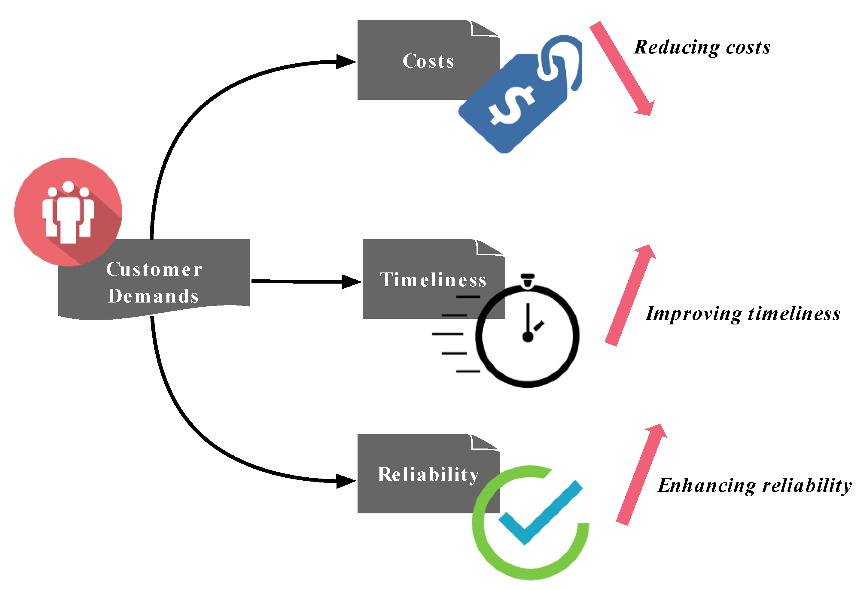
The road-rail intermodal routing problem aims at designing the best origin-to-destination routes that combine container trucks and container trains to enable customers to accomplish their transportation orders. It is much more complex than the famous vehicle routing problem, since two different transportation modes, i.e., road transportation (container trucks) and rail transportation (container trains), should be optimized in a combinatorial way in the same transportation network [21]. Satisfying customer demands is the foundation of the routing optimization, especially when the traditional transportation industry is trying its best to develop into the modern service industry [22]. Therefore, the road-rail intermodal routing investigated by this study is a customer-centred optimization. Generally, the customer demands can be summarized as in Figure 1 [18].
First of all, since the cost created in the logistics activities research is up to nearly 30–50% of the companies’ total production cost [5,8], reducing logistics cost is considered as an effective way for companies to make profits. This motivates the minimization of the costs paid for accomplishing the transportation orders as the optimization objective of the road-rail intermodal routing modelling. Such an objective is established in the modelling by all the relative literature.
Secondly, improving the transportation timeliness to realize on-time transportation is important for companies that need to distribute their materials or products through the extensive intermodal transportation network. In the era when large numbers of companies resort to just-in-time (JIT) strategy to minimize inventory, minimizing time does not always lead to the minimization of costs [23]. Therefore, besides reducing costs paid for accomplishing their transportation orders, they also expect goods delivery at the right time instead of traditional delivery using the least time, i.e., avoiding both early and late delivery [9]. Solving the question of how to formulate and further improve the customer demand on timeliness is thus an important goal related to enhancing the service level of the intermodal transportation and its routing optimization.
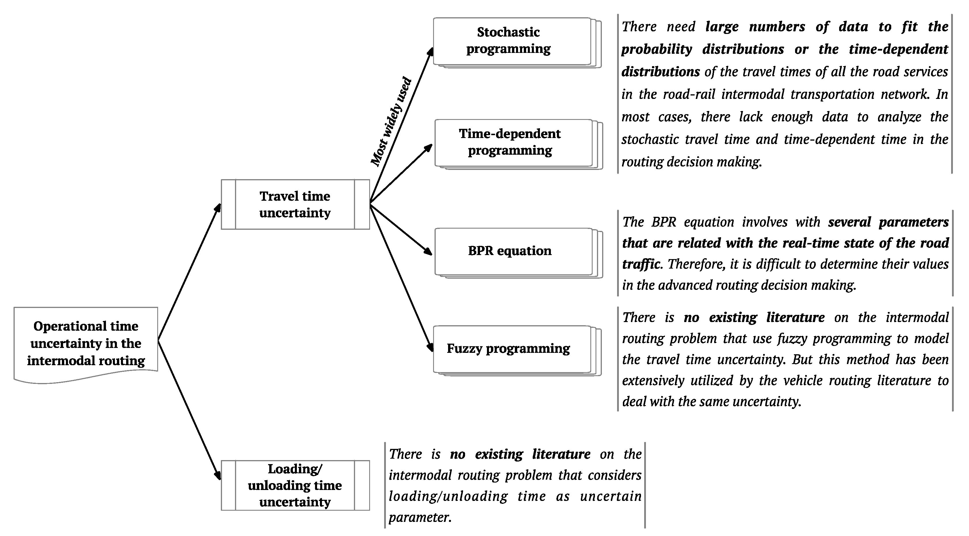
Last but not least, customers attach great importance to transportation reliability so that their transportation orders can be accomplished without disruptions, in order that they can reduce opportunity costs. Transportation reliability is significantly influenced by the uncertainty of the operations of the intermodal transportation network [24]. The operation uncertainty leads to time uncertainty. In the road-rail intermodal transportation network, the container trains are operated strictly by fixed schedules and usually get less disruptions [1,25,26]. Consequently, the time uncertainty of rail transportation can be neglected. As a result, in this study, road travel time and loading/unloading time are considered as the sources of time uncertainty. Road travel time uncertainty emerges due to traffic congestion, bad weather and accidents [1,27,28], while loading/unloading time uncertainty results from the unstable proficiency and state of staff that conduct loading/unloading operations, technical issues of the loading/unloading equipment and unpredictable tasks that occupy staff and equipment. These two sources of time uncertainty will not only influence the goods delivery but also disrupt the transshipment between road and rail. They should therefore be modeled in the road-rail intermodal routing optimization to improve the routing reliability.
Above all, in this study, we explore the road-rail intermodal routing problem that is directly oriented on satisfying the customer demands on reducing costs, improving timeliness and enhancing reliability. The contributions made by this study are fivefold.
(1) Fuzzy soft time windows are employed to model the due dates for accomplishing transportation orders. Maximizing the service level associated with the fuzzy soft time windows is set as part of the weighted objective of the road-rail intermodal routing model.
(2) Multiple sources of time uncertainty, i.e., road travel time uncertainty and loading/unloading time uncertainty, are comprehensively modeled by using fuzzy set theory.
(3) A hub-and-spoke network is utilized to model the road-rail intermodal transportation system with time-flexible container truck services and scheduled container train services.
(4) A fuzzy mixed integer nonlinear programming model is constructed to formulate the road-rail intermodal routing problem with fuzzy soft time windows and multiple sources of time uncertainty, and an exact solution approach combining defuzzification and linearization is developed.
(5) Sensitivity analysis and fuzzy simulation are adopted to quantify the effects of the fuzzy soft time windows and the uncertainty of road travel time and loading/unloading time on the road-rail intermodal routing optimization.
The remaining sections of this study are organized as follows. In Section 2, the existing literature on the intermodal routing problem is reviewed to demonstrate our improvements. In Section 3, we present the methods used to model the multiple sources of time uncertainty, the fuzzy soft time windows with respect to the due dates of accomplishing transportation orders and the road-rail intermodal hub-and-spoke transportation system. Based on the modelling foundation proposed in Section 3, we establish a fuzzy mixed integer nonlinear programming model in Section 4 for the road-rail intermodal routing problem that fully considers to satisfy the customer demands on costs, timeliness and reliability. In Section 5, considering the fuzziness of the model, defuzzification is first of all conducted to get a crisp model by using the fuzzy expect value model and fuzzy chance-constrained programming, so that decision makers can obtain crisp road-rail intermodal route planning. Then using the linearization technique developed in our previous study [1,25], linear reformulation of the nonlinear model is realized, so that global optimal solutions to the road-rail intermodal routing problem can be effectively obtained by using an exact solution algorithm that can be implemented by standard mathematical programming software. In Section 6, computational experiment is designed to verify the feasibility of the proposed methods. The effects of the fuzzy soft time windows and the uncertainty of road travel time and loading/unloading time on the road-rail intermodal routing optimization are discussed by using sensitivity analysis and fuzzy simulation. Finally, the conclusions of this study are drawn in Section 7.

2. Literature Review

There are large numbers of research articles that focus on the intermodal routing optimization. These studies have been very successful and so provide a solid foundation for us to continue this study. In order to fully understand the current progress of the existing literature on the customer-centred intermodal routing optimization, a systematic literature review on how existing literature deals with the customer demands is presented. Additionally, how to model the intermodal transportation system is a fundamental issue to optimize the associated routing problem. Consequently, the approaches for such issue will also be reviewed in this section.

2.1. Review on Modeling Customer Demand on Economy in the Intermodal Routing

Lowering costs reflects the customer demand on improving transportation economy and is always the most important objective of intermodal routing optimization. Even in the multi-objective optimization on the intermodal routing problem, for example, the hazardous materials routing problem [29,30] and fresh food routing problem [31], the economic objective plays an important role in the optimization. A few studies on the intermodal routing problem, e.g., Chang [8] and Moccia et al. [32], adopt a piecewise linear cost function that shows the effect of economies of scale to calculate the economic objective. However, the piecewise linear cost function is only dependent on the transported weight [8]. Actually, the costs are not only associated with transported weight, but also related to the time and distance. Moreover, it is difficult to determine the various parameters of the piecewise linear cost function in transportation practice. Therefore, it is not completely applicable to use the piecewise linear cost function to represent the economic objective function. Currently, the majority of the existing studies employ generalized costs to formulate the charges for accomplishing the transportation orders, e.g., Sun et al. [1,18,25,30], Ayar and Yaman [31], Hrušovský et al. [2] and Demir et al. [3]. Generalized costs have a structure shown as Figure 2 [30,33,34] and thus cover all the payment created in the activities of the intermodal transportation. In this study, we continue to use generalized costs to formulate the economic objective of road-rail intermodal routing problem.

2.2. Review on Modeling Customer Demand on Timeliness in the Intermodal Routing

As for the customer demand on improving transportation timeliness, there are various studies on intermodal routing problem that consider the “less time, the better” concept, and hence set minimizing the transportation time as their optimization objective, e.g., Chang [8], Vale and Ribeiro [21], Sun and Chen [35], Cai et al. [36], Xiong and Wang [37] and Xiong and Dong [38]. In these studies, a multi-objective optimization is used to deal with the intermodal routing problem, and minimizing the transportation time is of one of the multiple objectives of the modelling. Tradeoff between minimizing the transportation time and other objectives (e.g., minimizing transportation costs [8,35,36,37,38] or minimizing carbon emissions [21]) is made by using Pareto analysis. However, as emphasized by Dua and Sinha [9], minimizing transportation time is not always the best option to improve transportation timeliness, since nowadays the customers highly expect that their goods can be delivered at the right time to avoid both early and late delivery. In this case, the majority of the existing literature consider improving transportation timeliness by formulating due dates of accomplishing transportation orders. Currently, the methods to formulate the due dates can be summarized as in Figure 3.
As for the formulation methods shown in Figure 3, at the initial stage, using hard time points to describe the due dates is very popular in the intermodal routing optimization. Sun et al. [19,39], Verma and Verter [40] and Wang and Han [41] formulate the due date constraint based on the hard time point formulation that requires that the instants of accomplishing transportation orders by intermodal transportation should not be later than the prescribed due dates. Although using hard time points to formulate the due date constraint can avoid lateness of the delivery, early delivery might occur. Consequently, some studies on the intermodal routing problem propose the concept of soft due dates, so that penalty can be used to reduce the degree of both earliness and lateness of the delivery. Hrušovský et al. [2] and Demir et al. [3] use soft time points to represent the due dates. In their studies, the penalty cost is linear with the degree of the earliness or lateness. By lowering the penalty cost caused by earliness and lateness of the delivery through minimizing the economic objective, the on-time transportation can be enhanced.
As claimed by Sun et al. [42], time windows are more suitable and flexible to model the due dates by using lower and upper bounds to describe the customers’ opinions on the delivery that is neither too early nor too late. Currently, Zhang et al. [43] develop hard time windows to model the due dates and require that the transportation time of each order must fall into the time window. In fact, customers also accept the violation of the due date time windows to a certain degree [42,44,45]. Under this situation, soft time windows receive a lot of attention from the intermodal routing literature when discussing the formulation of due dates. Sun et al. [1,18,30] and Fazayeli et al. [46] explore the intermodal location-routing problem with due dates denoted by soft time windows. In Fazayeli et al.’s study, the penalty cost strategy that is the same as that of Hrušovský et al. [2] and Demir et al. [3] is used to optimize the timeliness of the intermodal transportation. In many cases, however, violation of the soft due date time windows does not lead to a penalty cost [44]. Moreover, it is difficult to determine the value of the unit penalty cost in transportation practice.
The due dates claimed by customers usually involve their subjective opinions [44]. The service level of the intermodal routing on timeliness significantly influences the customer satisfaction. When formulating soft time windows and the corresponding penalty cost strategy is infeasible, it is worthwhile to try to model the service level of the intermodal routing in order to further improve the timeliness by constructing an associated constraint or objective. The most popular method of building the function of customer satisfaction associated with subjective opinions is fuzzy set theory [45]. From that viewpoint of fuzzy set theory, the due dates can be modeled as fuzzy soft time windows that are expressed by trapezoidal fuzzy numbers [44,45]. The customer satisfaction on the instants when the transportation orders are accomplished can be measured by the fuzzy membership of the trapezoidal fuzzy numbers. Such measurement quantifies the service level of the intermodal routing. Currently, to the best of our knowledge, there is no existing literature that investigates the intermodal routing problem with fuzzy soft time windows. But such an idea gets widely discussed in the vehicle routing problem, e.g., Tang et al. [44], Lopez-Castro and Montoya-Torres [45], Ghannadpour et al. [47] and Xu et al. [48]. In this study, we will introduce the fuzzy soft time windows into the intermodal routing problem to improve the service level of the routing optimization. The optimization of the service level will be realized by setting service objective and constructing service level constraint.

2.3. Review on Modeling Customer Demand on Reliability in the Intermodal Routing

Transportation reliability is a measure of the containers being successfully delivered to the receivers by using the planned intermodal routes in actual transportation. It is highly influenced by uncertainty [49]. As explained in Section 1, operational time is the main source of the uncertainty. In the majority of the existing studies on the intermodal routing problem, travel time and loading/unloading time are treated as deterministic parameters. Sun et al. [50] pointed out that both overestimation and underestimation might exist if uncertain parameters are valued in a deterministic way, which will reduce the reliability of the intermodal routing.
However, the intermodal routing problem with operational time uncertainty (specifically, road travel time and loading/unloading time uncertainty in this study) does not receive enough of the highlights it deserves. A few relative studies can be found so far. The current research progress on the intermodal routing problem with operational time uncertainty is illustrated by Figure 4. Hrušovský et al. [2] and Demir et al. [3] explore the green intermodal routing problem with travel time uncertainty. Stochastic programming is employed by their study to model the uncertain travel time. Similar study on the sea-rail intermodal routing problem with stochastic travel time is then conducted by Zhao et al. [51], in which a chance-constrained stochastic approach is provided under the assumption that the travel time follows a normal distribution. Uddin and Huynh [24,52] also underline the importance of formulating road travel time uncertainty in improving the reliability of the road-rail intermodal routing, and develop a multicommodity model based on stochastic programming. Besides stochastic programming, Sun et al. [1] adopt the time-dependent travel time represented by the continuous piecewise linear function to describe the road travel time uncertainty caused by traffic congestion. Further they integrate the time-dependent road travel time with the intermodal routing problem. Resat and Turkay [17], Liu et al. [26] and Tang et al. [53] use the classical BPR (Bureau of Public Roads) equation to estimate the road travel time in road-rail intermodal transportation.
The above studies only consider the uncertainty of travel time, while neglecting the loading/unloading time uncertainty that also exists in the routing decision-making stage. Considering multiple sources of uncertainty however might help decision makers find improved intermodal routes [1]. As a result, in this study, we will consider both road travel time uncertainty and loading/unloading time uncertainty when modeling the road-rail intermodal routing, so that road-rail intermodal routes with improved reliability can be provided to decision makers.
Moreover, as indicated by Figure 4, stochastic programming, time-dependent programming and the BPR equation all have their own disadvantages in dealing with the uncertainty [27,54], which considerably reduces their feasibility in dealing with the optimization problems with uncertainty. To the best of our knowledge, fuzzy programming as an alternative method to address uncertainty has not been considered in the intermodal routing literature that involves uncertain issues. Based on the fuzzy set theory introduced by Zadeh [55], fuzzy programming has been widely considered as a useful tool to deal with uncertainty [56]. In the fuzzy programming, the uncertain parameters or variables can be effectively valued by the pessimistic, optimistic and most likely estimations from experts and decision makers based on their knowledge and experience [50]. Consequently, compared with the rest three methods, fuzzy programming does not rely on the size of the existing data or the real-time information of a system and is hence more flexible in practical decision making. Although less attention has been paid on the fuzzy programming in dealing with the intermodal routing problem with time uncertainty, it has already been employed by Sun et al. [1] to model capacity uncertainty and by Sun et al. [18] to formulate demand uncertainty in the intermodal routing problem, and shows good feasibility. Additionally, it has been widely adopted by the vehicle routing problem with travel time uncertainty, e.g., Zhang and Liu [27], Zarandi et al. [54] and Djadane et al. [57]. Since fuzzy programming can combine limited historical data with the expert knowledge and experience to effectively estimate the uncertainty, in this study, we will use fuzzy programming to model the multiple sources of time uncertainty that exist in the road-rail intermodal routing problem.

2.4. Review on Modeling Intermodal Transportation System

How to model the intermodal transportation system is the foundation of the routing optimization. First of all, an efficient intermodal transportation network where the routes are planned should be constructed. The consolidation of the intermodal transportation network is the most important factor that influences the efficiency of the transportation [6]. The four kinds of consolidation networks, i.e., point-to-point, line, collection-and-distribution and hub-and-spoke networks, can be seen from Macharis and Bontekoning’s work [6]. The hub-and-spoke network is widely acknowledged to be the most suitable consolidation network to construct the road-rail intermodal transportation system [18]. The superiority of the road-rail intermodal hub-and-spoke network is its systematic integration of the different advantages of the time-flexible road transportation and scheduled rail transportation in the pre haul-long haul-end haul transportation chain, which is stressed by Wang et al. [19] and Sun et al. [1,18,30].
However, modeling the road-rail transportation system as a hub-and-spoke network does not receive enough attention from researchers in the intermodal routing field. A few studies, e.g., Sun et al. [1,18] and Uddin Huynh [24], consider the hub-and-spoke structure as part of the transportation network when modeling the intermodal transportation system. Sun et al. [30] adopted the hub-and-spoke network to represent the road-rail intermodal transportation network when exploring the bi-objective optimization on the hazardous materials routing problem. Although such consolidation network is not very popular in the road-rail intermodal routing problem, it has had great importance attached to the intermodal transportation design problem, e.g., Wang et al. [19], Meng and Wang [58], Yang et al. [59], Lin and Chen [60,61] and Konings et al. [62]. Consequently, in this study, we will model the road-rail intermodal transportation system as a hub-and-spoke network and further optimize the associated road-rail intermodal routing problem.
Furthermore, the routing optimization is used to support the practical decision making on the transportation organization. As a result, the modeling of the road-rail intermodal transportation system should match the real world. As stated in Section 1, the intermodal routing problem is more complex than the vehicle routing problem, since it involves more than one transportation mode and different transportation modes are operated in different ways. In the road-rail transportation system, road transportation is time flexible, while rail transportation should be operated with fixed schedules [6,8]. Therefore, when modeling the road-rail intermodal routing problem, a combination of the two different transportation modes by transshipping operations at rail terminal (hubs) in the road-rail intermodal hub-and-spoke network should therefore follow the restrictions of the schedules of the selected container trains. Moreover, the arrival and departure of the containers carried by container trains should also observe the schedules.
At the beginning of the intermodal routing optimization, schedules are not formulated in the intermodal routing problem. The majority of the existing studies, e.g., Yiping et al. [36], Xiong and Wang [37], Xiong and Dong [38], Zhang et al. [43], Çakır [63], Chang et al. [64], consider that after arriving at the transshipping node by one transportation mode, the containers are immediately unloaded, then loaded on to another transportation mode once the unloading operation is finished, and finally depart from the transshipping node when the loading operation is finished. Since the schedules of some transportation modes really exist in the transportation practice and need to be modeled in the intermodal routing problem, modeling schedules become part of the routing optimization. A few studies, e.g., Hrušovský et al. [2], Demir et al. [3], Liu et al. [65] and Lin [66], formulate the scheduled departure instant constraint that the arrival instant of containers at the transshipping node should not be later than the scheduled departure instant of the successive transportation mode with schedules. Limited studies can be found that consider the scheduled service time window of transportation modes with schedules when optimizing the intermodal routing problem, e.g., Chang [8], Ayar and Yaman [31] and Moccia et al. [32]. In transportation practice, schedules regulate more than the departure instant and service/operation time window. As summarized by our previous study [1,25,30], in the road-rail intermodal transportation scenario, the schedules of rail transportation contain operation time windows, arrival instants and departure instants of freight trains at and from the rail terminals covered on their running routes as well as their operational periods. Therefore, in order to establish a road-rail intermodal transportation system that represents the real-world transportation organization, we will model the above-mentioned contents of schedules by referring to our previous study.

2.5. Review Summaries

As we can see from Section 2.1, Section 2.2, Section 2.3 and Section 2.4, the existing literature on the intermodal routing problem has shown that sustainable accomplishments have been achieved, especially in optimizing the customer demand on transportation economy. But as we can see from the literature review, research gaps still exist in the following aspects:
(1) Optimizing the customer demand on transportation efficiency by formulating due dates of accomplishing transportation orders in a more applicable way.
(2) Optimizing the customer demand on transportation reliability by modeling multiple sources of time uncertainty, i.e., road travel time uncertainty and loading/unloading time uncertainty, in a more feasible programming method.
(3) Modeling an efficient road-rail intermodal transportation system that also matches the real-world transportation organization to provide a solid foundation for the routing modelling.
In this study, we focus on the customer-centred freight routing optimization in the road-rail intermodal transportation network and aim at bridging these research gaps through the way that is presented in Section 1 (see the fivefold contributions made by this study).

3. Methodology

In this study, we extend the road-rail intermodal routing problem by modeling multiple sources of time uncertainty, i.e., road travel time and loading/unloading time uncertainty, to improve reliability and considering fuzzy soft time windows to improve service level associated with timeliness. The routing problem is further oriented on a road-rail intermodal hub-and-spoke transportation system. In this section, we present the methods for modeling time uncertainty, fuzzy soft time windows and the road-rail intermodal transportation system.

3.1. Modeling Time Uncertainty by Fuzzy Set Theory

As mentioned in Section 1, considering the limitation of using stochastic programming to deal with uncertainty, in this study, we adopt fuzzy set theory to model the two kinds of time uncertainty by using fuzzy numbers. In practical decision-making, different decision makers might hold different viewpoints on estimating the values of fuzzy parameters, including pessimistic, optimistic and most likely estimations [30,67].
Interval, triangular and trapezoidal fuzzy numbers can be used to represent fuzzy parameters [18,68]. In this study, we select triangular fuzzy numbers to model the above characteristics of the estimation of the fuzzy parameters (specifically, road travel time and loading/unloading time in this study) due to the following two reasons.
(1) Triangular fuzzy numbers are simpler and more flexible in the fuzzy arithmetic operations than the other two kinds of fuzzy numbers [69,70].
(2) Triangular fuzzy numbers can match the estimations held by different decision makers to fully reflect the practical decision-making scenario under fuzzy environment, which can be seen in Figure 5.
For a triangular fuzzy number t ˜ = ( t 1 ,   t 2 ,   t 3 ) representing fuzzy road travel time or fuzzy loading/unloading time, its three prominent points are defined as follows.
(1) t 1 is the most optimistic estimation, and corresponds to the best case that the traffic conditions of the road transportation are extremely good, or the loading/loading operations are conducted quite smoothly.
(2) t 2 is the most likely estimation, and corresponds to the most likely case that shows what the traffic conditions of the road transportation or the loading/unloading operations usually are.
(3) t 3 is the most pessimistic estimation, and corresponds to the worst case that the traffic conditions of the road transportation are extremely bad (for example, severe congestion occurs), or there are severe technical or operational issues that happen to disrupt the loading/unloading operations (for example, equipment breakdown happens).

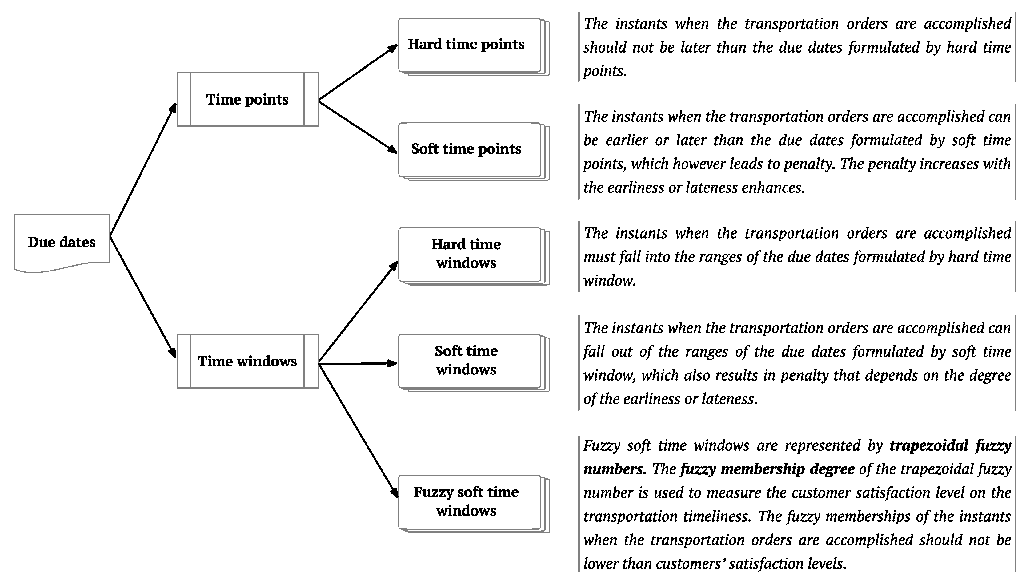
3.2. Modeling the Due Dates of Transportation Orders by Fuzzy Soft Time Windows

As stated in Section 1, in this study, we employ fuzzy soft time windows to model the due dates of accomplishing transportation orders, so that the timeliness of road-rail intermodal routing can be effectively improved. First of all, there need time intervals to represent the instants of accomplishing transportation orders that are neither too early nor too late for customers. When the instant of accomplishing a transportation order falls into such a time interval, the satisfaction of the customer reaches the highest. Otherwise the satisfaction will be reduced. Moreover, since the customers cannot accept that the transportation orders are accomplished too early or too lately. Therefore, the fuzzy soft time windows have lower bounds and upper bounds separately representing the earliest and latest instants that the customers can accept. Above all, the fuzzy soft time window has four prominent points, and shows the same representation as the trapezoidal fuzzy numbers. The fuzzy membership function of the trapezoidal fuzzy number can therefore be used to measure the customers’ satisfaction level [44]. A fuzzy soft time window can be denoted by T ˜ = ( T 1 ,   T 2 ,   T 3 ,   T 4 ) the fuzzy membership of which is illustrated by Figure 6. The four prominent points of a fuzzy soft time window are given as follows.
(1) T 1 is the endurable earliest instant of accomplishing a transportation order. The customer cannot accept the instant of accomplishing a transportation order that is earlier than T 1 .
(2) [ T 2 ,   T 3 ] is the preferred instant range of accomplishing a transportation order. The customer considers the transportation timeliness reaches its maximum, in other words, his or her satisfaction level reaches maximum (100%), if the instant of accomplishing a transportation order falls into [ T 2 ,   T 3 ] .
(3) T 4 is the endurable latest instant of accomplishing a transportation order. The customer cannot accept the instant of accomplishing a transportation order that is later than T 4 .
Given an instant of accomplishing a transportation order denoted by T , the corresponding satisfaction level μ ( T ) is calculated by Equation (1) [44].
μ ( T ) = { T T 1 T 2 T 1 T 1 T < T 2 1 T 2 T T 3 T 4 T T 4 T 3 T 3 < T T 4 0 otherwise
Under the above setting, it is acceptable that the instant of accomplishing a transportation order falls into [ T 1 ,   T 2 ] or [ T 3 ,   T 4 ] , which however reduces the customer’s satisfaction level. If the customer requires a satisfaction level that is no less than η , the endurable instant range of accomplishing the transportation order is [ T 2 η ,   T 3 η ] (see Figure 6), where T 2 η = η · ( T 2 T 1 ) + T 1 and T 3 η = T 4 η · ( T 4 T 3 ) according to Equation (1).
In this study, the service level associated with fuzzy soft time windows in the road-rail intermodal routing is optimized by the following two aspects.
(1) Maximizing the total service levels of all the transportation orders is set as part of the weighted objective of the routing model.
(2) A service level constraint is established to ensure the service level of each transportation order is not lower than a satisfaction degree requested by corresponding customer.

3.3. Modeling the Road-Rail Intermodal Transportartion System
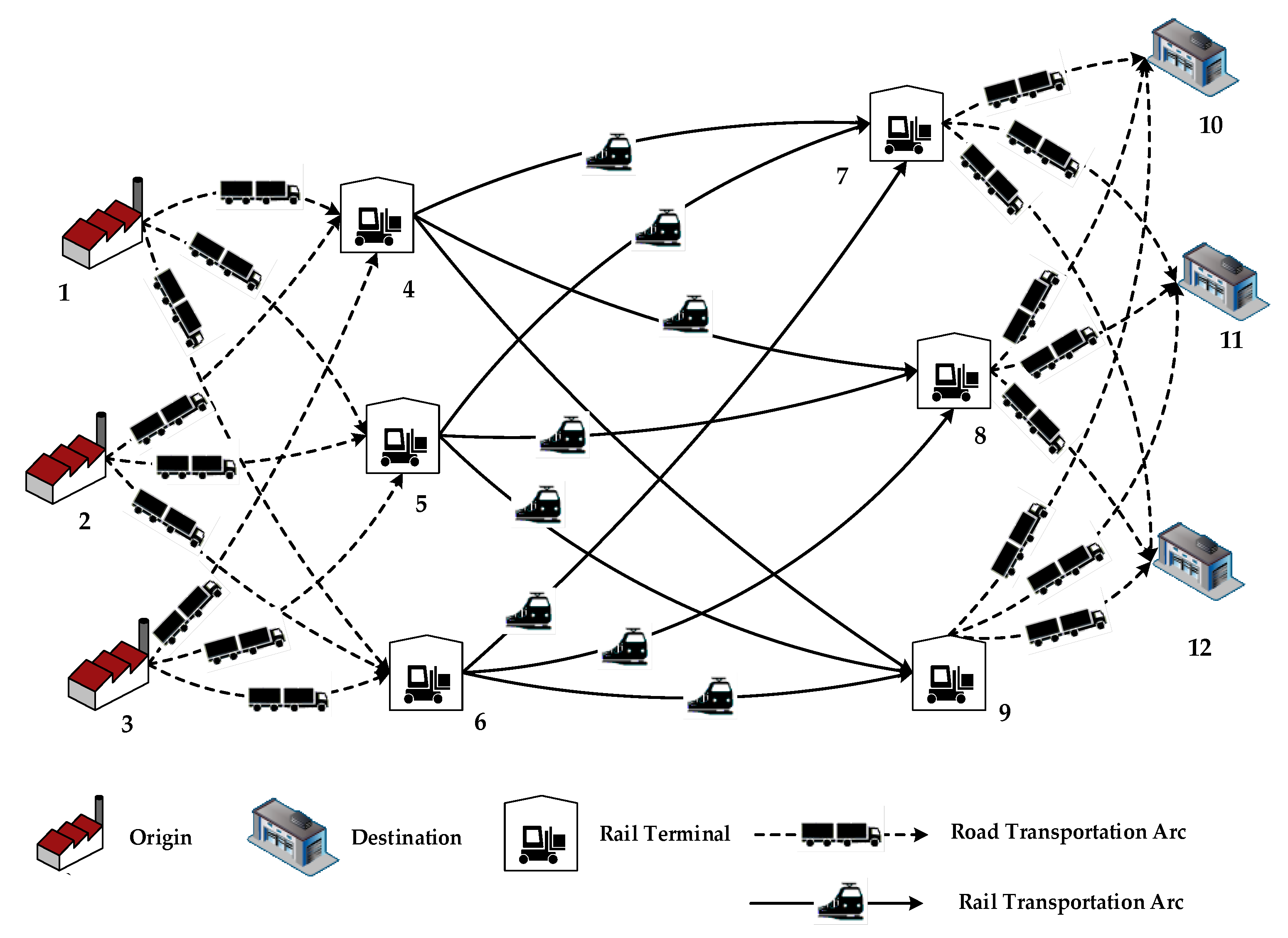
As claimed in Section 2, a hub-and-spoke network shown as Figure 7 is used to model the road-rail intermodal transportation system. Rail terminals installed with loading/unloading equipment are the hub where transshipment between container trucks and container trains is realized. Origins and destinations are the spokes, and are connected with rail terminals by container truck transportation [19,30]. If containers from various transportation orders at a rail terminal are gathered together, the operations of the rail terminal can be centralized to lead to economies of scale [19], which is the main advantage of the road-rail intermodal hub-and-spoke network.
Another issue is how to coordinate various transportation modes with different operational characteristics by routing to generate origin-to-destination intermodal routes that are feasible in both space and time. In the road-rail intermodal transportation system, road transportation is time flexible and thus offers good mobility, while rail transportation is operated by fixed schedules that regulate the operation time windows, arrival and departure instants of a container train at the rail terminals covered on its running route as well as its operational period [1,25,30].
Therefore, in order to design feasible road-rail intermodal routes, the operations of container trucks should coordinate with the schedules of the container trains, especially during the “Arriving → Transshipping → Departing” operation process at rail terminals. Figure 8 indicates the road-rail intermodal transportation process in a hub-and-spoke network that captures the operational characteristics of road and rail transportation [30]. Such process will be formulated in the modelling.
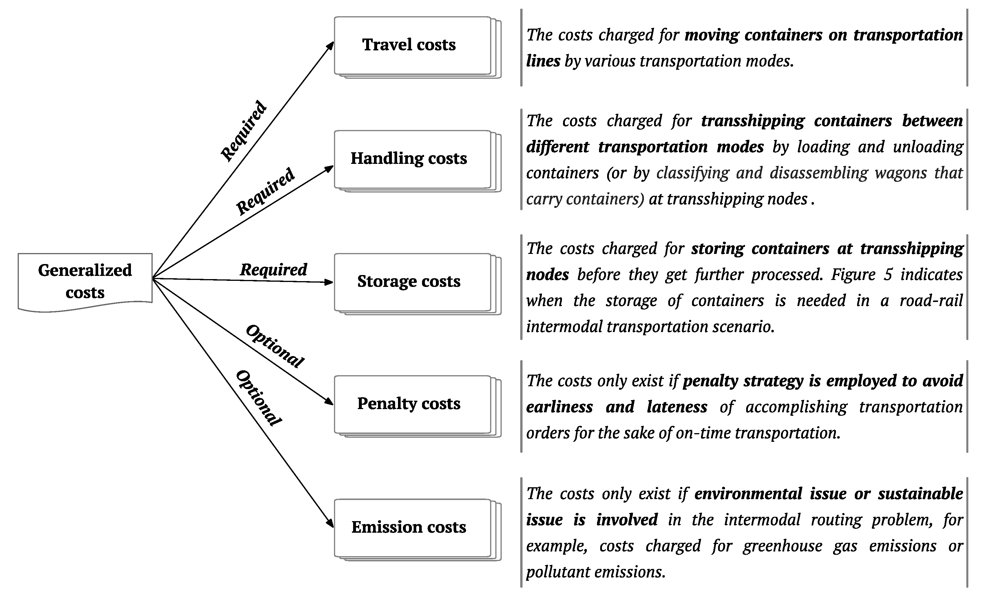
In the transportation process illustrated by Figure 8, there are three kinds of costs that are created in the road-rail intermodal transportation, i.e., travel costs, loading and unloading costs and storage costs. The economic objective of the road-rail intermodal routing optimization is also to minimize the sum of these costs paid for accomplishing all the transportation orders.
As we can see from Figure 8, the arrival instants of containers by trucks are related to the road travel time, and the storage time of containers at rail terminals are determined by the arrival instants of containers and the loading/unloading time. Obviously, the uncertainty of road travel time and loading/unloading time lead to uncertainty of the arrival instant and storage time. Therefore, there are two parameters (i.e., road travel time and loading/unloading time) and two decision variables (i.e., arrival instants of containers by trucks and storage time of containers at rail terminals) in the optimization model that are uncertain.

4. A Fuzzy Mixed Integer Nonlinear Programming Model

4.1. Modelling Characteristics

The optimization on the routing problem is based on a given framework that contains a series of modelling characteristics [10,30,71]. According to Sun et al. [30,71] and Kumar et al. [10], the modelling of a freight routing problem should comprehensively consider the characteristics listed in Figure 9. It also systematically indicates how we select the modelling characteristics to establish our optimization model.

4.2. Symbols Used to Establish the Model

The symbols used to establish the optimization model are similar to the ones presented in our previous study that provides a solid modelling foundation for us to carry out this study [30] and are introduced in Table 1. It should be noted that there are two fuzzy decision variables in the model, and the their fuzziness has been explained in Section 3.3.

4.3. Objective Functions of the Road-Rail Intermodal Routing Problem

  • Economic Objective
    minimize   p P ( i ,   j ) A m S i j c m · q p · d i j m · x i j m p + p P j N i N i m S i j e m · q p · x i j m p + p P j N k N i + n S j k e n · q p · x j k n p + p P ( i ,   j ) A m R a i l i j f s t o r e · q p · z ˜ i j m p
    The economic objective is to minimize the total generalized costs of accomplishing all the transportation orders that contains travel costs, loading and unloading costs and storage cost.
  • Service Objective
    maximize   p P μ p ( E [ y ˜ d p p + i N d p m T r u c k i d p t ˜ d p m · q p · x i d p m p ] )
    The service objective is to maximize the service levels of all the transportation orders to improve the customers’ satisfaction degrees. Since the road travel time and unloading time are fuzzy, the instants of accomplishing transportation orders are also fuzzy. In this study, we use the fuzzy expected value of the instant of accomplishing a transportation order as the input to calculate the service level.
  • Weighted Objective
    minimize   p P ( i ,   j ) A m S i j c m · q p · d i j m · x i j m p + p P j N i N i m S i j e m · q p · x i j m p + p P j N k N i + n S j k e n · q p · x j k n p + p P ( i ,   j ) A m R a i l i j f s t o r e · q p · z ˜ i j m p W · p P μ p ( E [ y ˜ d p p + i N d p m T r u c k i d p t ˜ d p m · q p · x i d p m p ] )
    The economic objective and service objective can be linearly combined together by distributing a weight to the service objective. The combination is shown as Equation (4). The value of the weight is determined by the decision makers according to their preference to the service objective.

4.4. Constraints of the Road-Rail Intermodal Routing Problem

i N i m S i j x i j m p k N i + n S j k x j k n p = { 1 j = o p 0 j N \ { o p ,   d p } 1 j = d p p P
m S i j x i j m p 1 p P ( i ,   j ) A
Equation (5) is the flow conservation constraint to ensure the integrity of an origin-to-destination route for each transportation order. The combination of Equation (5) and Equation (6) ensures the containers in each transportation order are unsplittable.
( t p 0 + t 1 o p n · q p + t o p k n 1 y 1 k p ) · x o p k n p = 0 p P k N o p + n T r u c k o p k
( t p 0 + t 2 o p n · q p + t o p k n 2 y 2 k p ) · x o p k n p = 0 p P k N o p + n T r u c k o p k
( t p 0 + t 3 o p n · q p + t o p k n 3 y 3 k p ) · x o p k n p = 0 p P k N o p + n T r u c k o p k
[ i N j m R a i l i j ( t w j m + t 1 j m · q p ) · x i j m p + t 1 j n · q p + t j d p n 1 y 1 d p p ] · x j d p n p = 0 p P j N d p n T r u c k j d p
[ i N j m R a i l i j ( t w j m + t 2 j m · q p ) · x i j m p + t 2 j n · q p + t j d p n 2 y 2 d p p ] · x j d p n p = 0 p P j N d p n T r u c k j d p
[ i N j m R a i l i j ( t w j m + t 3 j m · q p ) · x i j m p + t 3 j n · q p + t j d p n 3 y 3 d p p ] · x j d p n p = 0 p P j N d p n T r u c k j d p
y ˜ k p = ( y 1 k p ,   y 2 k p ,   y 3 k p ) p P k N / ( { o p } N d p )
Equations (7)–(9) are used to calculate the three prominent points of the fuzzy arrival instant of containers at the rail terminal by container trucks after departing from the origin (pre-haul). Equations (10)–(13) calculate the three prominent points of the fuzzy arrival instant of containers at the destination by container trucks after departing from the rail terminal (end-haul). After obtaining the prominent points, the fuzzy arrival instant represented by a triangular fuzzy number can be determined by Equation (13).
[ max { t w j n ( y 1 j p + i N j m S i j t 1 j m · q p · x i j m p ) ,   0 } z 3 j k n p ] · x j k n p = 0 p P ( j ,   k ) A n R a i l i j
[ max { t w j n ( y 2 j p + i N j m S i j t 2 j m · q p · x i j m p ) ,   0 } z 2 j k n p ] · x j k n p = 0 p P ( j ,   k ) A n R a i l i j
[ max { t w j n ( y 3 j p + i N j m S i j t 3 j m · q p · x i j m p ) ,   0 } z 1 j k n p ] · x j k n p = 0 p P ( j ,   k ) A n R a i l i j
z ˜ j k n p = ( z 1 j k n p ,   z 2 j k n p ,   z 3 j k n p ) p P ( j ,   k ) A n R i j
The three prominent points of the fuzzy storage time at the rail terminal can be further calculated by Equations (14)–(16) to obtain the triangular fuzzy number representation of the fuzzy storage time by Equation (17).
y ˜ j p + i N j m S i j t ˜ j m · q p · x i j m p + z ˜ j k n p + t ˜ j n · q p t w j n + · x j k n p + ϵ · ( 1 x j k n p ) p P ( j ,   k ) A n R a i l i j
In Equation (18), ϵ is a large enough positive constant. Equation (18) ensures that the loading completion instant of the containers at the rail terminal should not be later than the operation cutoff instant (upper bound of the operation time window) of the selected container train. Obviously, Equation (18) is a fuzzy constraint.
p P q p · x i j m p c a p i j m ( i ,   j ) A m S i j
Equation (19) is the transportation capacity constraint that ensures the total volume loaded on a common container train or a common group of truck fleets does not exceed the allowable capacity.
μ p ( E [ y ˜ d p p + i N d p m T r u c k i d p t ˜ d p m · q p · x i d p m p ] ) η p p P
Equation (20) is the service level constraint that ensures the service level associated with the expected instant of accomplishing each transportation order should not be lower than the customer’s satisfaction degree.
x i j m p { 0 ,   1 } p P   ( i ,   j ) A m S i j
y 3 i p y 2 i p y 1 i p 0 p P i N
z 3 j k n p z 2 j k n p z 1 j k n p 0 p P ( i ,   j ) A m R a i l i j
Equations (21)–(23) are the domain constraints of the variables.

5. Solution Approaches

The aim of designing the approaches is to generate an equivalent mixed integer linear programming model, so that the global optimal solutions to the road-rail intermodal routing problem can be obtained by using an exact solution algorithm run by mathematical programming software. Consequently, the solution approaches contain the following two parts:
(1) Defuzzification that is used to generate a crisp optimization model that can provide decision makers with crisp route planning.
(2) Linearization that is used to generate an equivalent linear programming model that can be effectively solved by using an exact solution algorithm to get the global optimal solutions.

5.1. Defuzzification of the Fuzzy Constraint

Equation (18) is a fuzzy constraint, since it contains fuzzy decision variables y ˜ j p and z ˜ j k n p as well as fuzzy parameters t ˜ j m and t ˜ j n . To realize the defuzzification of Equation (18), fuzzy chance-constrained programming is applied in this study to reformulate the fuzzy constraint. Compared with the fuzzy possibility and fuzzy necessity measures, the fuzzy credibility measure is self-dual and can ensure that a fuzzy event must hold if its credibility equals 1 while it must fail if its credibility equals 0 [27,50]. Therefore, fuzzy credibility is more suitable than the other two measures to be used to construct a fuzzy chance constraint.
Based on the fuzzy credibility measure, the fuzzy chance constraint of Equation (18) is as Equation (24). In this equation, α is a confidence level determined by decision makers subjectively. Equation (24) ensures the credibility of the fuzzy event in Cr { } should not be lower than a given credibility level.
Cr { y ˜ j p + i N j m S i j t ˜ j m · q p · x i j m p + z ˜ j k n p + t ˜ j n · q p t w j n + · x j k n p + ϵ · ( 1 x j k n p ) } α p P ( j ,   k ) A n R a i l i j
The left-hand function of Equation (24) can be rewritten as Equation (25).
Cr { ( t w j n + · x j k n p + ϵ · ( 1 x j k n p ) ( y 3 j p + i N j m S i j t 3 j m · q p · x i j m p + z 3 j k n p + t 3 j n · q p ) , t w j n + · x j k n p + ϵ · ( 1 x j k n p ) ( y 2 j p + i N j m S i j t 2 j m · q p · x i j m p + z 2 j k n p + t 2 j n · q p ) , t w j n + · x j k n p + ϵ · ( 1 x j k n p ) ( y 1 j p + i N j m S i j t 1 j m · q p · x i j m p + z 1 j k n p + t 1 j n · q p ) ) 0 }
As indicated by Cao and Lai [72] and Zheng and Liu [27], given a deterministic number r and a triangular fuzzy number d ˜ = ( d 1 ,   d 2 ,   d 3 ) , there exists Equation (26).
Cr { d ˜ r } = { 1 if   r d 1 2 d 2 d 1 r 2 ( d 2 d 1 ) if   d 1 r d 2 d 3 r 2 ( d 3 d 2 ) if   d 2 r d 3 0 if   r d 3
Furthermore, based on Equation (26), Cr { d ˜ r } α equals Equations (27) and (28) according to proof proposed by Sun et al. [1] and Wang et al. [19].
2 α · d 2 ( 2 α 1 ) · d 3 a    if   0 α 1 2
2 ( 1 α ) · d 2 + ( 2 α 1 ) · d 1 a    if   1 2 < α 1
Accordingly, the fuzzy chance constraint Equation (24) can be reformulated as Equations (29) and (30) that are crisp and linear.
2 α · [ t w j n + · x j k n p + ϵ · ( 1 x j k n p ) ( y 2 j p + i N j m S i j t 2 j m · q p · x i j m p + z 2 j k n p + t 2 j n · q p ) ] ( 2 α 1 ) · [ t w j n + · x j k n p + ϵ · ( 1 x j k n p ) ( y 1 j p + i N j m S i j t 1 j m · q p · x i j m p + z 1 j k n p + t 1 j n · q p ) ] if   0 α 1 2 p P ( j ,   k ) A n R a i l i j
2 ( 1 α ) · [ t w j n + · x j k n p + ϵ · ( 1 x j k n p ) ( y 2 j p + i N j m S i j t 2 j m · q p · x i j m p + z 2 j k n p + t 2 j n · q p ) ] ( 1 2 α ) · [ t w j n + · x j k n p + ϵ · ( 1 x j k n p ) ( y 3 j p + i N j m S i j t 3 j m · q p · x i j m p + z 3 j k n p + t 3 j n · q p ) ] if   1 2 < α 1 p P ( j ,   k ) A n R a i l i j

5.2. Defuzzification of the Fuzzy Objective

The optimization objective is fuzzy, because it contains fuzzy decision variables y ˜ j p and z ˜ j k n p . Therefore, it is also necessary to realize the defuzzification of the fuzzy objective in order to obtain crisp solutions to the road-rail intermodal routing problem. Currently, there are two defuzzification methods that can be used to deal with the fuzzy objective, including fuzzy expected value model and the fuzzy chance-constrained programming. However, there is no solid evidence demonstrating that one method is better than the other or the two methods have same performance. As a result, in this study, we will use both defuzzification methods to address the fuzzy objective and also test their performance in dealing with the road-rail intermodal routing problem with time uncertainty in the case study section.

5.2.1. Using the Fuzzy Expected Value Model

The expected value of a triangular fuzzy number d ˜ = ( d 1 ,   d 2 ,   d 3 ) is expressed by Equation (31) [73].
E [ d ˜ ] = d 1 + 2 d 2 + d 3 4
The fuzzy expected value model is widely acknowledged to be an effective approach to deal with a fuzzy objective [18]. It aims at minimizing or maximizing the expected value of the fuzzy objective. According to Equation (30), the fuzzy expected value of the total storage costs for all transportation orders can be obtained by Equation (32).
E [ p P ( i ,   j ) A m R a i l i j f s t o r e · q p · z ˜ i j m p ] = p P ( i ,   j ) A m R a i l i j f s t o r e · q p · E [ z ˜ i j m p ] = p P ( i ,   j ) A m R a i l i j f s t o r e · q p · z 1 j k n p + 2 z 2 j k n p + z 3 j k n p 4
The fuzzy expected value of the weighted objective is therefore given by Equations (33) and (34) by replacing the fuzzy storage costs with the corresponding fuzzy expected value.
minimize   p P ( i ,   j ) A m S i j c m · q p · d i j m · x i j m p + p P j N i N i m S i j e m · q p · x i j m p + p P j N k N i + n S j k e n · q p · x j k n p + p P ( i ,   j ) A m R a i l i j f s t o r e · q p · z 1 j k n p + 2 z 2 j k n p + z 3 j k n p 4 W · p P μ p ( v p 4 )
v p = y 1 d p p + i N d p m T r u c k i d p t 1 d p m · q p · x i d p m p + 2 ( y 2 d p p + i N d p m T r u c k i d p t 2 d p m · q p · x i d p m p ) + y 3 d p p + i N d p m T r u c k i d p t 3 d p m · q p · x i d p m p p P

5.2.2. Using Fuzzy Chance-Constrained Programming

Fuzzy chance-constrained programming can be also used to deal with the fuzzy objective [74]. In this case, Equation (4) can be reformulated as Equations (35) and (36) where ψ is a non-negative auxiliary variable.
minimize   p P ( i ,   j ) A m S i j c m · q p · d i j m · x i j m p + p P j N i N i m S i j e m · q p · x i j m p + p P j N k N i + n S j k e n · q p · x j k n p + ψ W · p P μ p ( v p 4 )
Cr { p P ( i ,   j ) A m R a i l i j f s t o r e · q p · z ˜ i j m p ψ } α
Similar to the crisp reformulation of Equation (24), Equation (36) is equivalent to Equations (37) and (38).
2 α · p P ( i ,   j ) A m R a i l i j f s t o r e · q p · z 2 i j m p + ( 1 2 α ) · p P ( i ,   j ) A m R a i l i j f s t o r e · q p · z 1 i j m p ψ if   0 α 1 2
2 ( 1 α ) · p P ( i ,   j ) A m R a i l i j f s t o r e · q p · z 2 i j m p + ( 2 α 1 ) · p P ( i ,   j ) A m R a i l i j f s t o r e · q p · z 3 i j m p ψ if   1 2 < α 1

5.3. Linear Reformulation of the Service Objective

The service level function μ p ( v p 4 ) is a continuous piecewise linear function. Therefore, the service objective function p P μ p ( v p 4 ) is nonlinear.
Constrained by Equation (20), for p P , v p 4 must fall into range [ T W p 1 ,   T W p 4 ] , and can only fall into only one of its three sub ranges shown as Figure 10. First of all, we define a 0–1 auxiliary variable w g p : if v p 4 falls into range g ( g G = { 1 ,   2 ,   3 } ), w g p = 1 , otherwise, w g p = 0 . Hence we have Equations (39) and (40).
g G w g p = 1 p P
w g p { 0 ,   1 } p P g { 1 ,   2 ,   3 }
Then we distribute non-negative auxiliary variables ξ g p and ξ g p + to the lower bound and upper bound of range g , and so we have Equations (41)–(43).
ξ g p + ξ g p + = w g p p P g { 1 ,   2 ,   3 }
ξ g p 0 p P g { 1 ,   2 ,   3 }
ξ g p + 0 p P g { 1 ,   2 ,   3 }
Furthermore, v p 4 can be expressed by Equation (44).
v p 4 = g G ( ξ g p · T W p g + ξ g p + · T W p g + 1 ) p P
By using Equation (44) to replace v p 4 in the service objective function p P μ p ( v p 4 ) , we have the following formula.
p P μ p ( v p 4 ) = p P μ p ( g G ( ξ g p · T W p g + ξ g p + · T W p g + 1 ) ) = p P g G μ p ( ξ g p · T W p g + ξ g p + · T W p g + 1 ) = p P g G [ μ p ( ξ g p · T W p g ) + μ p ( ξ g p + · T W p g + 1 ) ] = p P g G [ ξ g p · μ p ( T W p g ) + ξ g p + · μ p ( T W p g + 1 ) ] = p P ( ξ 1 p + + ξ 2 p + ξ 2 p + + ξ 3 p )
As a result, the linearized crisp weighted objective function under the fuzzy expected value model is as in Equation (46).
minimize   p P ( i ,   j ) A m S i j c m · q p · d i j m · x i j m p + p P j N i N i m S i j e m · q p · x i j m p + p P j N k N i + n S j k e n · q p · x j k n p + p P ( i ,   j ) A m R a i l i j f s t o r e · q p · z 1 j k n p + 2 z 2 j k n p + z 3 j k n p 4 W · p P ( ξ 1 p + + ξ 2 p + ξ 2 p + + ξ 3 p )
Under fuzzy chance-constrained programming, the linearized crisp weighted objective function is as in Equation (47).
minimize   p P ( i ,   j ) A m S i j c m · q p · d i j m · x i j m p + p P j N i N i m S i j e m · q p · x i j m p + p P j N k N i + n S j k e n · q p · x j k n p + ψ W · p P ( ξ 1 p + + ξ 2 p + ξ 2 p + + ξ 3 p )

5.4. Linear Reformulation of the Nonlinear Constraints

According to Sun et al. [25], nonlinear constraints Equations (7)–(12) can be linearized as Equations (48)–(59).
t p 0 + t 1 o p n · q p + t o p k n 1 y 1 k p ϵ · ( x o p k n p 1 ) p P k N o p + n T r u c k o p k
t p 0 + t 1 o p n · q p + t o p k n 1 y 1 k p ϵ · ( 1 x o p k n p ) p P k N o p + n T r u c k o p k
t p 0 + t 2 o p n · q p + t o p k n 2 y 2 k p ϵ · ( x o p k n p 1 ) p P k N o p + n T r u c k o p k
t p 0 + t 2 o p n · q p + t o p k n 2 y 2 k p ϵ · ( 1 x o p k n p ) p P k N o p + n T r u c k o p k
t p 0 + t 3 o p n · q p + t o p k n 3 y 3 k p ϵ · ( x o p k n p 1 ) p P k N o p + n T r u c k o p k
t p 0 + t 3 o p n · q p + t o p k n 3 y 3 k p ϵ · ( 1 x o p k n p ) p P k N o p + n T r u c k o p k
i N j m R a i l i j ( t w j m + t 1 j m · q p ) · x i j m p + t 1 j n · q p + t j d p n 1 y 1 d p p ϵ · ( x j d p n p 1 ) p P j N d p n T r u c k j d p
i N j m R a i l i j ( t w j m + t 1 j m · q p ) · x i j m p + t 1 j n · q p + t j d p n 1 y 1 d p p ϵ · ( 1 x j d p n p ) p P j N d p n T r u c k j d p
i N j m R a i l i j ( t w j m + t 2 j m · q p ) · x i j m p + t 2 j n · q p + t j d p n 2 y 2 d p p ϵ · ( x j d p n p 1 ) p P j N d p n T r u c k j d p
i N j m R a i l i j ( t w j m + t 2 j m · q p ) · x i j m p + t 2 j n · q p + t j d p n 2 y 2 d p p ϵ · ( 1 x j d p n p ) p P j N d p n T r u c k j d p
i N j m R a i l i j ( t w j m + t 3 j m · q p ) · x i j m p + t 3 j n · q p + t j d p n 3 y 3 d p p ϵ · ( x j d p n p 1 ) p P j N d p n T r u c k j d p
i N j m R a i l i j ( t w j m + t 3 j m · q p ) · x i j m p + t 3 j n · q p + t j d p n 3 y 3 d p p ϵ · ( 1 x j d p n p ) p P j N d p n T r u c k j d p
According to Sun et al. [25], nonlinear constraints Equations (14)–(16) are equivalent to the following linear equations.
z 3 j k n p t w j n ( y 1 j p + i N j m S i j t 1 j m · q p · x i j m p ) + ϵ · ( x j k n p 1 ) p P ( j ,   k ) A n R a i l i j
z 3 j k n p ϵ · x j k n p p P ( j ,   k ) A n R a i l i j
z 2 j k n p t w j n ( y 2 j p + i N j m S i j t 2 j m · q p · x i j m p ) + ϵ · ( x j k n p 1 ) p P ( j ,   k ) A n R a i l i j
z 2 j k n p ϵ · x j k n p p P ( j ,   k ) A n R a i l i j
z 1 j k n p t w j n ( y 3 j p + i N j m S i j t 3 j m · q p · x i j m p ) + ϵ · ( x j k n p 1 ) p P ( j ,   k ) A n R a i l i j
z 1 j k n p ϵ · x j k n p p P ( j ,   k ) A n R a i l i j
The service level constraint Equation (20) is also nonlinear, since it contains continuous piecewise linear function. Based on the description in Section 3.2, it can be reformulated as the following two equations that are both linear.
v p 4 η p · ( T W p 2 T W p 1 ) + T W p 1 p P
v p 4 T W p 4 η p · ( T W p 4 T W p 3 ) p P

5.5. Equivalent Mixed Integer Linear Programming Model

After defuzzification and linearization, the fuzzy mixed integer nonlinear model can be modified into two kinds of MILP models. The process that generates the two models is illustrated by Figure 11.
As we can see from Figure 11, two different crisp linear programming models can be obtained after using two different defuzzification methods to deal with the fuzzy objective and employing same linearization techniques to remove the nonlinearity. We use the fuzzy expected value model to defuzzy the initial fuzzy objective to obtain the MILP model I, and the fuzzy chance-constrained programming to generate the MILP model II. The differences of the two models are that they have different crisp objective functions and the MILP model II has two more auxiliary constraints (i.e., Equations (37) and (38)) deriving from the process of using fuzzy chance-constrained programming to deal with the fuzzy objective. Apart from Equations (37) and (38), the two MILP models share the same constraints.

6. Computational Experiment

We modify the numerical case designed in our previous study [30] to make it match the specific routing problem discussed by this study, and use the modified case to demonstrate the feasibility of proposed methods in dealing with the road-rail intermodal routing problem with fuzzy soft time windows and multiple sources of time uncertainty. The detailed description of the modified numerical case is presented in Appendix A (see Figure A1 and Table A1, Table A2 and Table A3 for details). The following works will also be untaken in this section in addition to demonstrating the feasibility:
(1) Exploring whether and how fuzzy soft time windows and fuzziness of both road travel time and loading/unloading time influence the road-rail intermodal routing optimization.
(2) Comparing the fuzzy expected value model and fuzzy chance-constrained programming in dealing with the fuzzy objective.
(3) Helping decision makers to identify the optimal value of confidence level α , so that a crisp road-rail intermodal transportation scheme can be provided to them.

6.1. Computational Environment

In this study, we use the standard Branch-and-Bound algorithm that is a famous exact solution algorithm in operations research to solve the two equivalent MILP models that formulate the specific routing problem discussed by this study. The Branch-and-Bound algorithm is run by the mathematical programming software LINGO version 12.0 [75]. All the computation is performed on a ThinkPad Laptop with Intel Core i5-5200U, 2.20 GHz CPU, and 8 GB RAM.
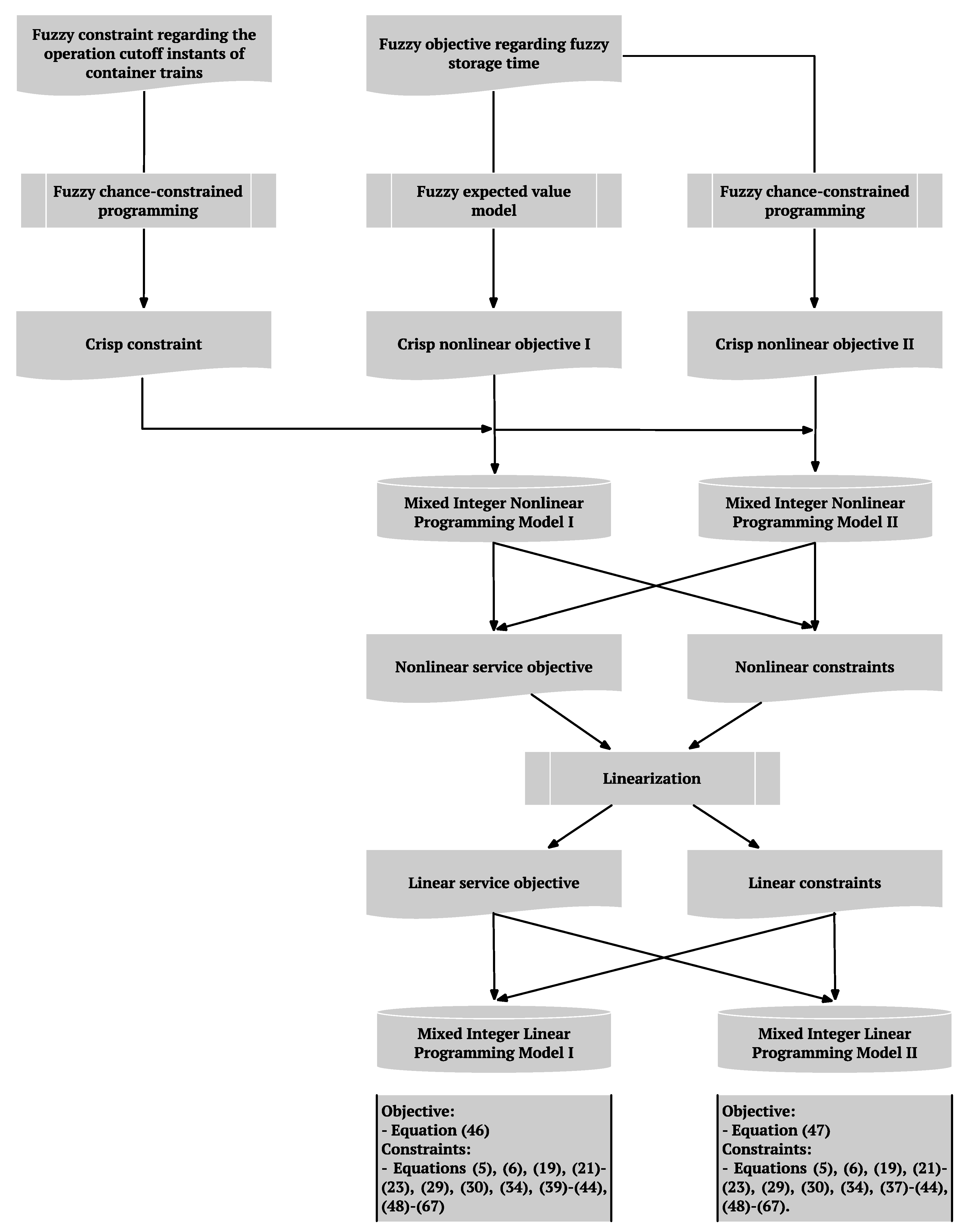
In this study, we provide two MILP models to solve problem. MILP model I uses fuzzy expected value model to deal with the fuzzy objective, while MILP model II employs fuzzy chance-constrained programming. Apart from the differences deriving from the defuzzification of the fuzzy objective, the two MILP models yield the same formulations. When using two MILP models to optimize the road-rail intermodal problem, the computational scale is shown in Table 2. As we can see from Table 2, MILP model II has two more variables than MILP model I, because non-negative auxiliary variable ψ emerges twice (one in the crisp objective Equation (47), and one in constraint Equation (37) or (38)) during the defuzzification of the fuzzy objective to obtain MILP model II, while there is no auxiliary variable generated when obtaining the crisp objective of MILP model I. Moreover, MILP model II has two more constraints than MILP model I, since the defuzzification for generating the crisp objective of MILP model II lead to two auxiliary constraints, including the constraint regarding the non-negativity of auxiliary variable ψ and the auxiliary constraint Equation (37) (or (38)). However, MILP model I does not generate any auxiliary constraints during the defuzzification of fuzzy objective.
When the confidence level α is set to 0.9, the service levels η p ( p P ) are set to 0.7 and the weight distributed to the service objective is set to 1000, the computational times of the models in 10 times computation are presented as follows. MILP model I has computational times that vary from 33 s to 34 s with an average value of 33.4 s in the 10 times computation. As for MILP model II, the maximum and minimum computational times are 26 s and 25 s, respectively. The average computational time of MILP model II is 25.6 s, which saves ~23.4% of the computational time compared with MILP model I. Therefore, using the Branch-and-Bound algorithm to solve the two MILP models to generate the best solutions to the routing problem can be accomplished within quite a short time. MILP model II that uses fuzzy chance-constrained programming to deal with the fuzzy objective shows better efficiency than MILP model I that uses the fuzzy expect value model to address the fuzzy objective.

6.2. Sensitivity Analysis of the Routing Optimization with Respect to the Weight of the Service Objective

The weight distributed to the service objective reflects the decision makers’ preference for the improvement on the transportation timeliness. In this study, we analyze the sensitivity of the routing optimization with respect to the weight associated with the service objective to reveal the relationship between the two optimization objectives. The following analysis is under the setting that confidence level α is set to 0.9 and service levels η p ( p P 
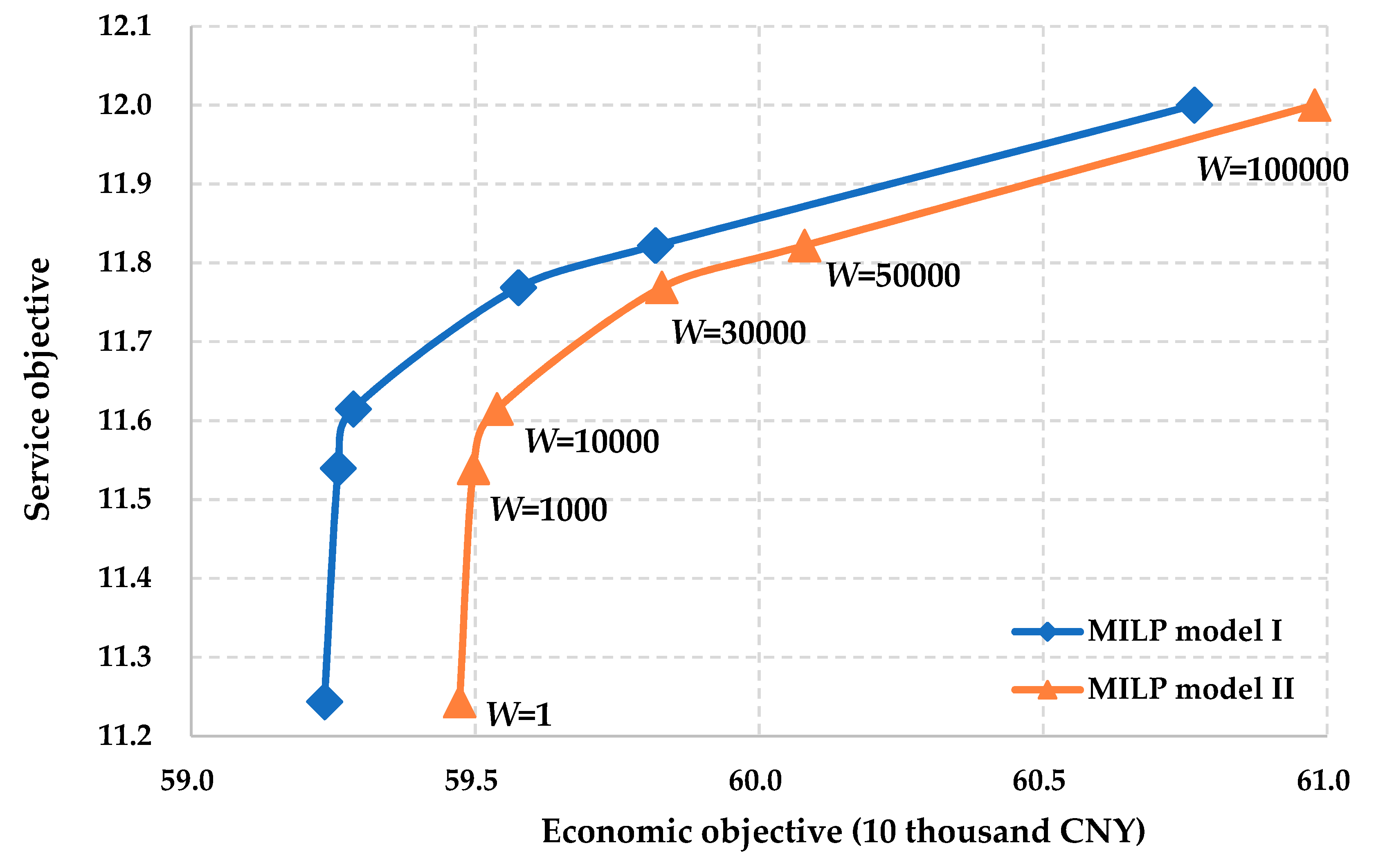
) are set to 0.7. The changes of the two objectives with respect to the weight, i.e., the Pareto frontiers to the bi-objective optimization on the road-rail intermodal routing problem, are indicated by Figure 12.
It can be observed from Figure 12 that by enhancing the weight distributed to the service objective, the value of the economic objective increases, which means that the transportation economy is reduced. Contrary to the transportation economy, the increase of the weight leads to the improved transportation timeliness, since the value of the service objective increases. Consequently, the economic objective and service objective of the road-rail intermodal routing problem cannot reach their respective optimum simultaneously, and enhancing one objective will worsen the other. A solution with minimum costs does not yield maximum service level. As a result, the road-rail intermodal routing problem yields non dominated solutions (i.e., Pareto solutions) instead of dominated solutions.
As shown in Figure 12, it is impossible to simultaneously satisfy the customer demands on transportation economy and timeliness by planning the road-rail intermodal routes. A tradeoff should therefore be made between the economic and service objectives based on the decision makers’ preference for the service improvement when planning the road-rail intermodal routes. The Pareto frontiers shown in Figure 12 can help decision makers to select the preferred solution. In practical decision making, decision makers can utilize the multiple-criteria decision-making methods, e.g., AHP method [76] and TOPSIS method [77], to preciously select the Pareto solution that best matches the decision-making situation.
Moreover, it can be noticed that MILP model II yields larger values of the economic objective than MILP model I, while the two models have the same values of the service objective. Although the two models have different values of the economic objective, the planned best road-rail intermodal routes given by them are exactly the same, which is demonstrated in the following Section 6.5.2. This leads to the same values of the service objective of the two models, since they share the same service objective function. However, the economic objective functions of the two models are different, which results in the difference of the values of the economic objective between the two models.

6.3. Sensitivity Analysis of the Routing Optimization with Respect to the Service Level

Besides the weight distributed to the service objective, the service level is also set by the decision makers manually. Its settings might influence the optimization results. In this study, we also use sensitivity analysis to explore its effect on the routing. We first of all set the weight as 1000 and the confidence level as 0.9. Then we modify service levels η p ( p P 
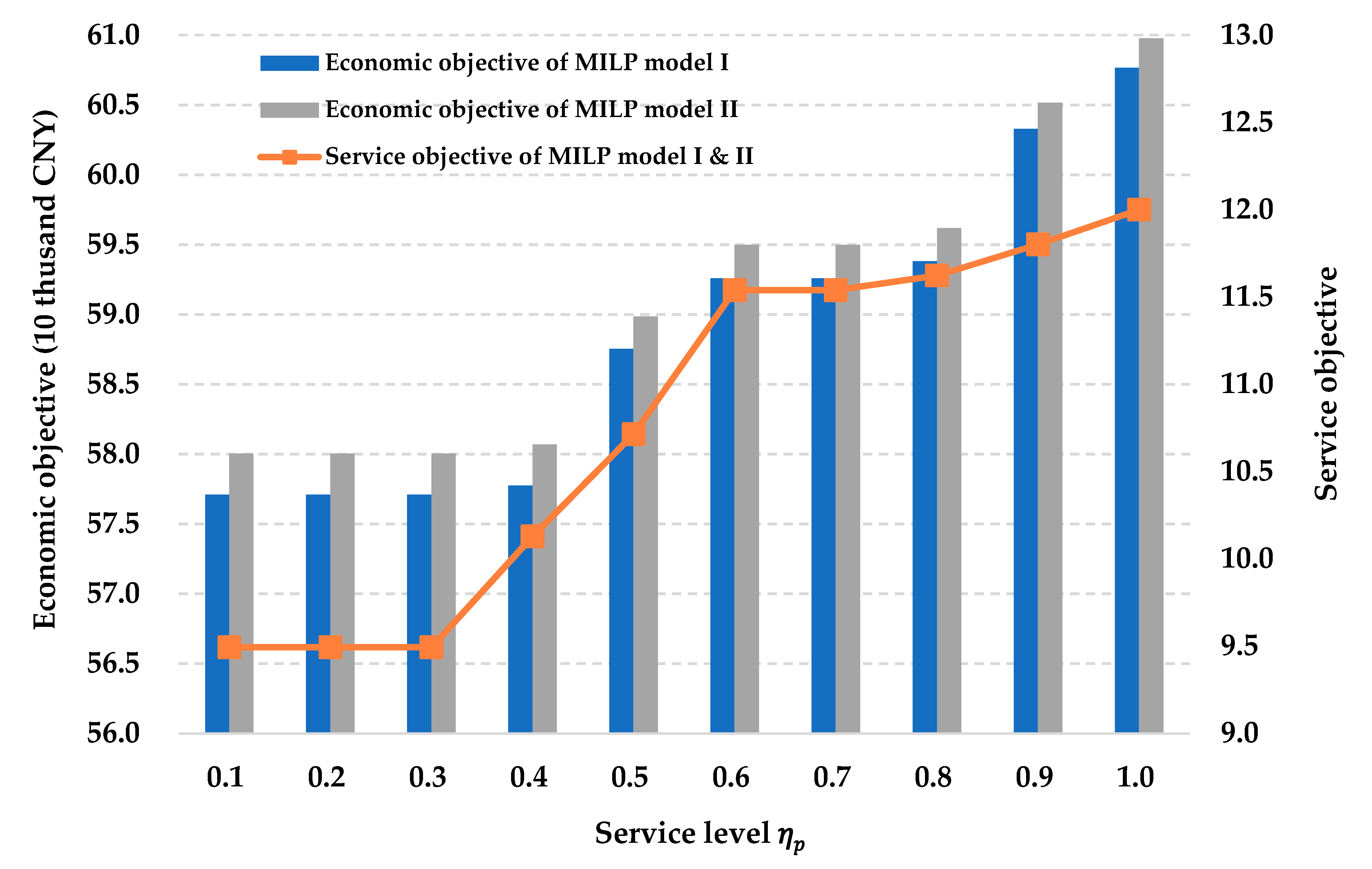
) from 0.1 to 1.0 with a step of 0.1, and calculate the best solutions corresponding to each value of the service level by solving MILP model I and MILP model II. The results of the sensitivity analysis are shown as Figure 13.
Figure 13 indicates that the road-rail intermodal routing optimization is sensitive to the service level. As we can see from Figure 13, by increasing the service level η p , both the values of the economic objective and service objectives show a growth tendency, which means that the transportation timeliness of the routing is getting improved, while its transportation economy is getting worse. Enhancing the service level shows an effect on the routing optimization that is the same as improving the weight distributed to the service objective.
Therefore, when customers prefer or propose a higher service level for accomplishing their transportation orders, enhancing the service level η p will help decision makers to find the best road-rail intermodal routes with improved transportation timeliness, on condition that customers could accept more costs paid for accomplishing transportation orders. With the help of Figure 13, decision makers can determine the value of the service level η p in a more objective way in order to avoid that the service level is overestimated and the economy of the routing is considerably reduced.
As well as the tendency shown in Figure 12, Figure 13 also shows that MILP model II provides larger values of the economic objective than MILP model I and the two models have same values of service objective. The reasons that lead to the tendency indicated by Figure 13 are same to the ones that result in Figure 12. Figure 13 points out that although the variation of the service level η p leads to the modification of the planned best routes, the two models always generate the same solutions under each value of the service level η p .

6.4. Sensitivity Analysis of the Routing Optimization with Respect to the Confidence Level

The confidence level α is another important parameter that is determined by decision makers according to their subjective preference. In this study, we set the weight distributed to the service objective as 1000 and the service level η p ( p P ) as 0.5. Under the above situation, we analyze the sensitivity of the routing optimization with respect to the confidence level. We vary the confidence level α 
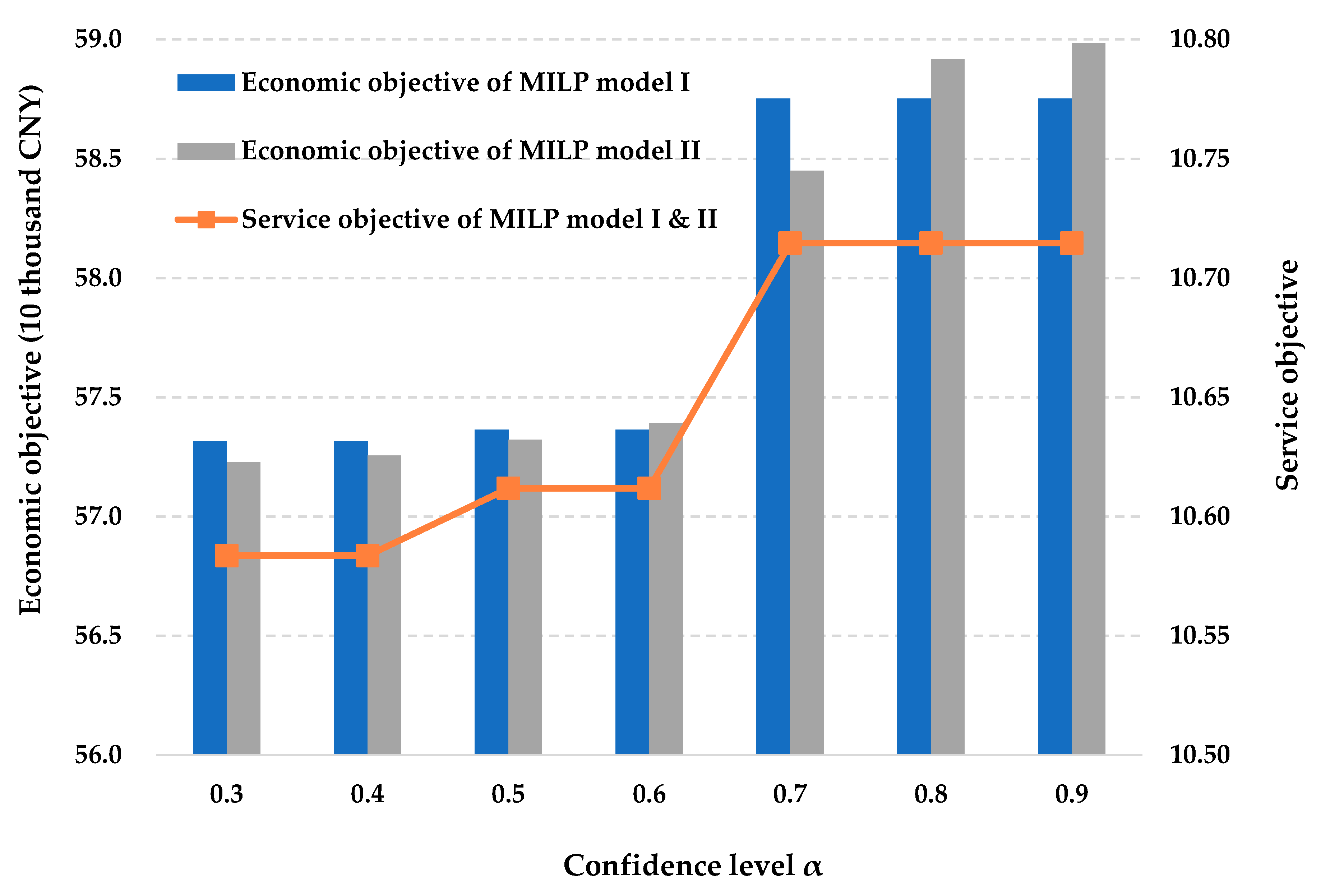
from 0.3 to 0.9 with a step of 0.1, and generate the best solutions to the routing problem by solving the two MILP models. The results of the sensitivity analysis are illustrated by Figure 14. It should be noted that there is no feasible solution that can be found when the confidence level α is set to 1.0.
As we can see from Figure 14, the road-rail intermodal routing optimization is sensitive to the confidence level, and increasing the confidence level leads to the increase of both economic objective and service objective. Since the larger confidence level means higher transportation reliability, Figure 14 also reveals that improving the transportation reliability will help to improve its transportation timeliness.
However, the value of the economic objective also increases with respect to the confidence level, which means that the transportation economy of the routing is in conflict with its transportation reliability. If customers prefer a road-rail intermodal route plan with higher transportation reliability, they should spend more on accomplishing their transportation orders. Figure 14 provides a solid foundation for decision makers to make effective tradeoffs among the economic objective, service objective and transportation reliability in order to avoid that the overestimation of one objective significantly reduces other objectives in the practical decision making.
Moreover, similar to Figure 12 and Figure 13, in the sensitivity analysis summarized in Figure 14, the two MILP models yield same service objective. However, their economic objectives do not provide the same value, and the value of the economic objective of MILP model II is not always larger than that of MILP model I. Figure 14 shows such tendency due to the same reasons that motivate the tendencies shown in Figure 12 and Figure 13. Moreover, as we can see from Figure 14, the two models yield the same route plan under each value of the confidence level, which is similar to the tendency shown in Figure 13.

6.5. Fuzzy Simulation to Gain the Crisp Road-Rail Intermodal Route Plan

In practical routing decision making, the decision makers who include transportation experts, transportation companies and customers will first of all determine the weight distributed to the service objective and the lowest service level that customers can accept. In this case, we set η p as 0.5 and W as 1000. Then if they want to obtain a crisp road-rail intermodal route plan, the confidence level that influences whether the routes are feasible in practice should be determined. Furthermore, the decision makers also need to determine which MILP model is more suitable. Considering the above decision making requirements, we design a fuzzy simulation method to help decision makers overcome the above issues in order to generate the best crisp road-rail intermodal route plan.
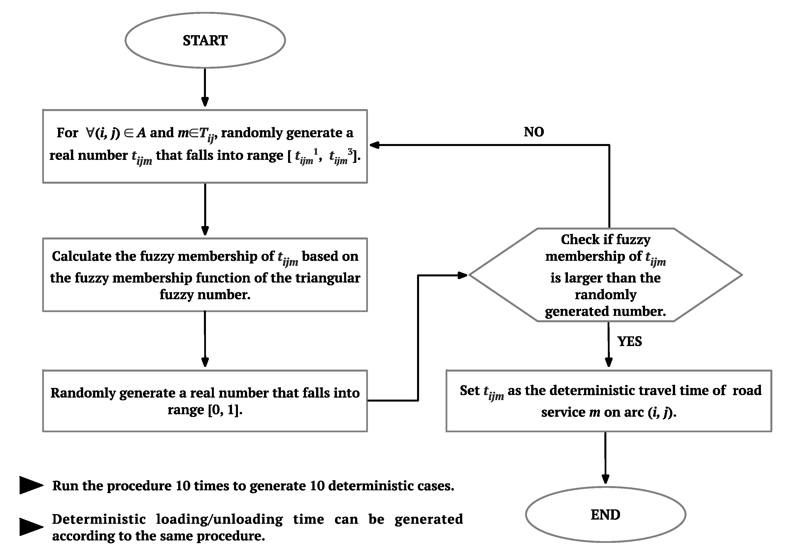
In this study, we randomly generate 10 sets of the deterministic road travel times and loading/unloading times according to the fuzzy membership function of the triangular fuzzy number as shown in Figure 5. Then we can obtain 10 deterministic cases that can be used to test the performances of different confidence levels and the two MILP models. The fuzzy simulation is run according to Figure 15 [1,50].

6.5.1. Testing the Feasibility of the Planned Best Road-Rail Intermodal Routes in the Deterministic Cases

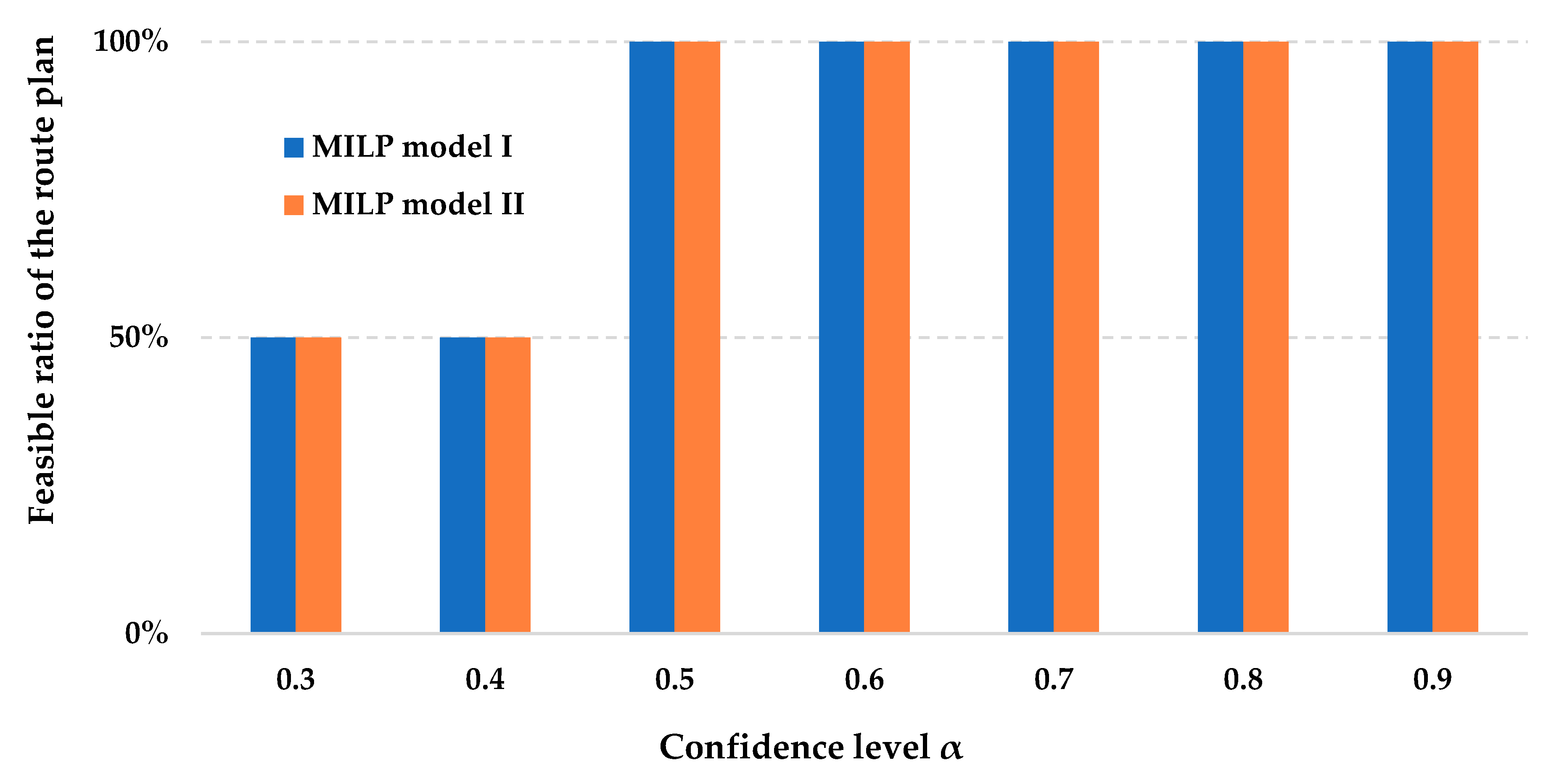
In this study, we first of all test the feasibility of the road-rail intermodal routes provided by the fuzzy programming models under different confidence levels in the 10 deterministic cases. When moving the containers along the planned road-rail intermodal routes in the deterministic cases, the route plan is feasible if the constraints of the upper bounds of the operation time windows of covered container trains (i.e., the deterministic formulation of Equation (18)) and the capacity constraints are satisfied. Otherwise, the route plan is infeasible and failed, which means that the transportation orders cannot be accomplished by using the planned routes. The feasible ratios of the route plans provided by the two MILP models under difference confidence levels in the 10 deterministic cases are shown in Figure 16.
As we can see from Figure 16, the route plans generated by solving the two MILP models show the same feasibility ratios in the 10 deterministic cases, regardless of the values of the confidence level. Furthermore, Figure 16 shows that with the increase of the confidence level, the feasibility ratios of the route plans, i.e., the transportation reliability of the routing, tend to be improved. However, in the cases set by this study, the improvement is not very sensitive.
When the confidence level is set to 0.5, 0.6, 0.7, 0.8 or 0.9, the route plans are feasible in all the deterministic cases. In the practical routing decision making, customers always demand that their transportation orders can be accomplished successfully by the planned routes to avoid rerouting that might cause much higher costs [1]. Therefore, as for the case study in this article, considering the customer demand on transportation reliability, the confidence level can be 0.5, 0.6, 0.7, 0.8 or 0.9.

6.5.2. Analyzing the Gaps Between the Planned Best Road-Rail Intermodal Routes and the Actual Best Routes in the Deterministic Cases

In the 10 deterministic cases, we replace the fuzzy parameters and fuzzy variables in the model presented in Section 4 with their deterministic forms, and thus get a deterministic road-rail intermodal routing model that can be linearized by using the linearization techniques given in Section 5. Consequently, the actual best road-rail intermodal routes in the 10 deterministic cases can be generated by solving the deterministic model.
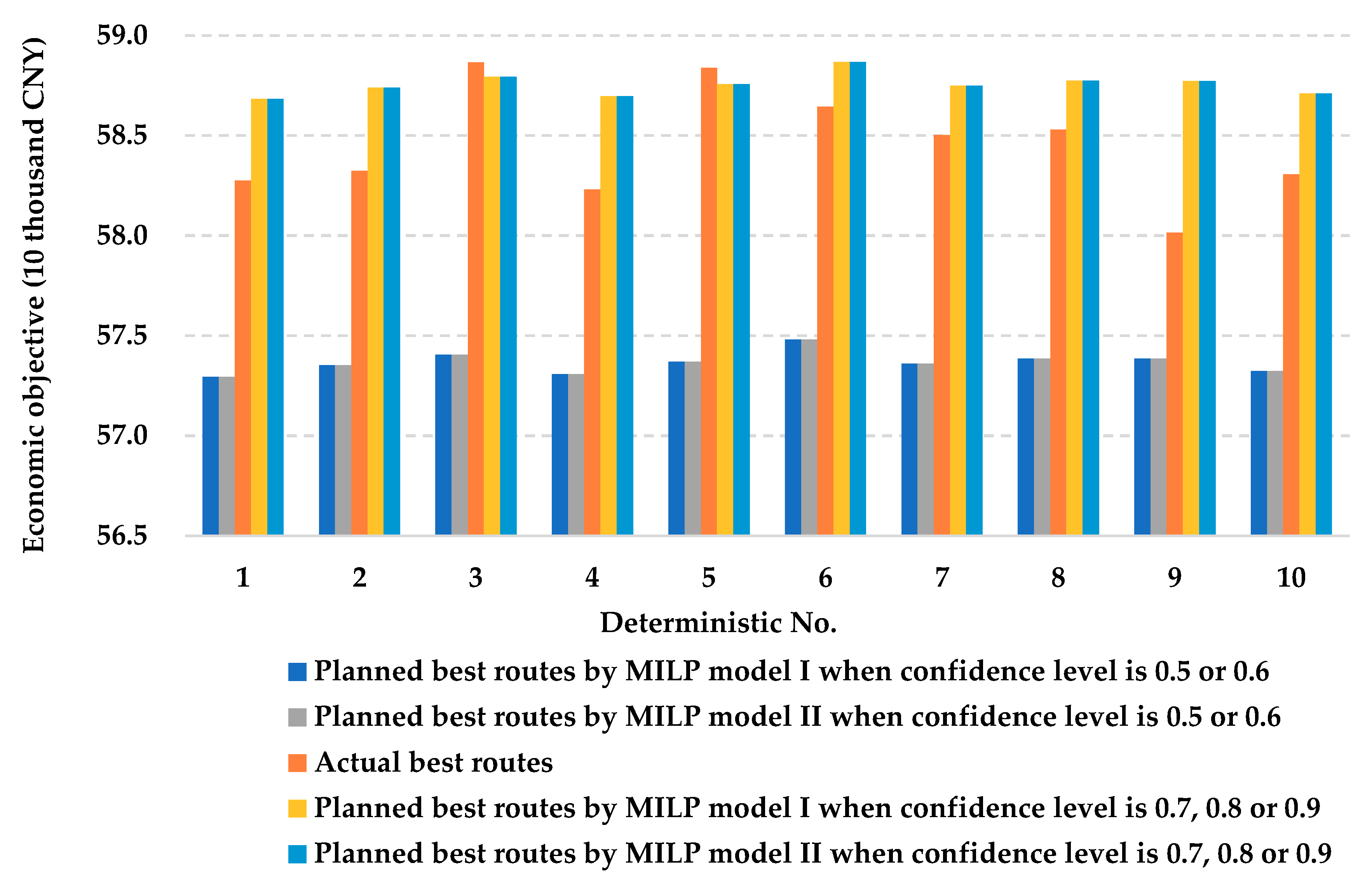
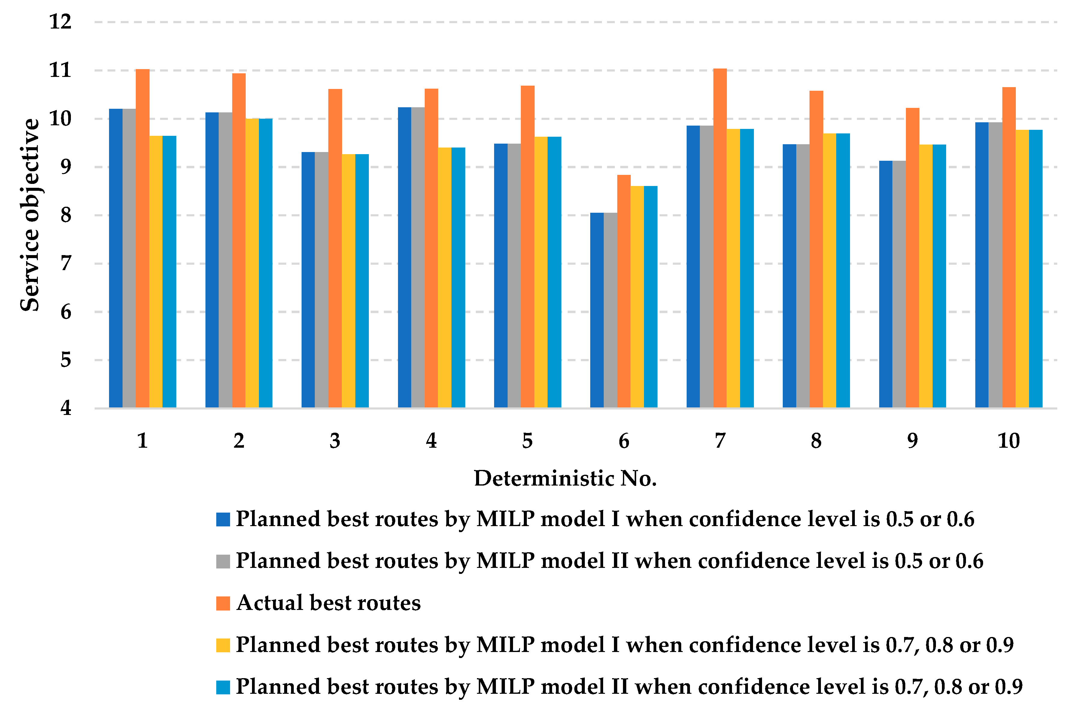
We can also calculate the values of the economic objective and the service objective of the planned best road-rail intermodal routes when they are used to move containers in the 10 deterministic cases. Then we can compare the gaps between planned best road-rail intermodal routes with the actual best routes in the 10 deterministic cases. The computational results are indicated by Figure 17 and Figure 18.
Shown as Figure 17 and Figure 18, we notice that the two MILP models yield the same computational results. Consequently, we can draw the conclusion that the performances of the two MILP models in dealing with the specific routing problem are the same. Either of them can be used to optimize the problem.
Based on the computation results shown in Figure 17 and Figure 18, we can calculate the root mean square (RMS) of the objectives of the planned best routes provided by MILP model I with respect to the objectives of the actual best routes in the 10 deterministic cases. The calculation results which are based on the associated RMS are given in Table 3.
Compared with the confidence level of 0.5 and 0.6, the MILP model I with the confidence levels of 0.7, 0.8 or 0.9 can significantly bridge the economic objective gap by ~65.5% by slightly extending the service objective gap by ~6.7%. As a result, when using the MILP model I to optimize the road-rail intermodal routing problem, the confidence level is recommended to be 0.7, 0.8 or 0.9. Above all, as for the numerical case introduced in the Appendix A, the best road-rail intermodal routes that can be used in the real-world transportation under η p = 0.5 and W = 1000 can be planned by solving any one of the two MILP models illustrated by Figure 11 with confidence level of 0.7, 0.8 or 0.9.
Furthermore, when confidence level is set to 0.5, MILP model II is converted into the deterministic optimization model used by the existing literature to deal with the road-rail intermodal routing with time certainty [25]. In the studies on the deterministic intermodal routing problem, the road travel time and loading/unloading time are valued in a deterministic way, i.e., by most likely estimations [18,23,25,30,37,43]. Therefore, indicated by Table 3, compared with the solutions generated by the deterministic optimization model, MILP models (i.e., models for the road-rail intermodal routing problem with time fuzziness) can obtain the crisp best road-rail intermodal routes that better match the actual best situation in the transportation practice. And considering the multiple sources of time uncertainty helps to improve the overall performance of the road-rail intermodal routing.

7. Conclusions

In this study, we focus on modeling and optimizing a customer-centred freight routing problem in the road-rail intermodal hub-and-spoke network with fuzzy soft time windows and multiple sources of time uncertainty. The following contributions are made by this study in order to improve the problem optimization:
(1) We employ fuzzy soft time windows to represent the due dates of accomplishing transportation orders. Maximizing the service level associated with the fuzzy soft time windows is set as the optimization objective and a service level constraint is also established, so that the transportation timeliness can be improved.
(2) We simultaneously consider the road travel time uncertainty and loading/unloading time uncertainty in the road-rail intermodal routing problem. The combination of the multiple sources of time uncertainty helps to enhance the transportation reliability of the routing.
(3) We model the road-rail intermodal transportation system as a hub-and-spoke network that contains time-flexible road transportation and scheduled rail transportation.
(4) We propose a bi-objective mixed integer nonlinear programming model the objectives of which are addressed by a weighting method to formulate the specific routing problem discussed in this study. By using the fuzzy expected value model, fuzzy chance-constrained programming and linearization techniques, two equivalent mixed integer linear programming models are generated and can be effectively solved by mathematical programming software.
In the case study, we make full use of sensitivity analysis and fuzzy simulation to quantify the effects of the fuzzy soft time windows and time uncertainty on the routing optimization. The following managerial implications can be deduced.
(1) The economic objective and service objective are in conflict with each other, i.e., the routing optimization cannot satisfy the customer demands on economy and timeliness simultaneously. An effective tradeoff between the two objectives can be made by using the Pareto frontier to the bi-objective optimization problem.
(2) When customers prefer or propose higher service levels for accomplishing their transportation orders, enhancing service level η p will help decision makers to find the best road-rail intermodal routes with improved transportation timeliness, on condition that customers could accept more costs paid for accomplishing transportation orders.
(3) Time uncertainty (fuzziness in this study) has significant effect on the routing optimization. A larger confidence level that means higher transportation reliability leads to improved service level (i.e., transportation timeliness), however, worsens the transportation economy of the routing.
(4) The fuzzy expected value model has the same performance as the fuzzy chance-constrained programming in dealing with the fuzzy objectives.
(5) By using the sensitivity analysis and fuzzy simulation designed in this study, decision makers can identify the best value(s) of the confidence level to provide a crisp road-rail intermodal route plan to the customers.
In the future work, we will first devote to exploring the green road-rail intermodal routing problem that considers to optimize the carbon dioxide emissions. We will discuss the green routing problem under different carbon emission regulations, including carbon tax regulation and carbon cap-and-trade regulation. The performances of the two regulations will be compared. Additionally, we will try to add other sources of uncertainty, e.g., demand uncertainty and capacity uncertainty, into the routing problem to further enhance the transportation reliability. Last but not least, developing a heuristic algorithm to efficiently solve the large-scale road-rail intermodal routing problem that is an NP-hard problem is also a direction of our future work.

Author Contributions

Y.S. proposed the topic explored in this paper. Y.S. developed the mathematical model proposed the solution strategy for the problem. Y.S. and X.L. designed the numerical case. Y.S. and X.L. conducted the computation, sensitivity analysis and fuzzy simulation in the case study. Y.S. and X.L. wrote the paper. X.L. thoroughly reviewed and improved the paper. Both authors have discussed and contributed to the manuscript. Both authors have read and approved the final manuscript.

Funding

This research was funded by the Shandong Provincial Natural Science Foundation of China, grant number ZR2019BG006, the Project for Humanities and Social Sciences Research of Ministry of Education of China, grant number 19YJC630149, and the Shandong Provincial Higher Educational Social Science Program of China, grant number J18RA053.

Acknowledgments

The authors would like to thank Cyril Bernard Lucas from the United Kingdom for his remarkable contribution to helping us polish the language of this manuscript.

Conflicts of Interest

The authors declare no conflict of interest.

Appendix A

The numerical case used in this study is modified from our previous study [30]. The detailed description of the case is presented as follows. It should be noted that the same container trains in different periods are treated as different transportation services and are indexed by different indexes.
Figure A1. A road-rail intermodal hub-and-spoke network.
Mathematics 07 00739 g0a1
Table A1. The schedules of the container trains in the network.
Container TrainsTrain RoutesOperation Start Instants at OriginsOperation Cutoff Instants at OriginsOperation Start Instants at DestinationsCapacities in TEUPeriods in Train per DayTravel Distances in km
1(4, 7)1530403001184
2(4, 7)623323501184
3(4, 8)520313801210
4(4, 8)321344001210
5(4, 9)926423201280
6(4, 9)1431463001280
7(5, 7)824353351193
8(5, 7)1329413551193
9(5, 8)725354001185
10(5, 8)1026373251185
11(5, 9)018322921178
12(5, 9)625352701178
13(6, 7)1130472901315
14(6, 7)1429503151315
15(6, 8)421323621236
16(6, 8)826403451236
17(6, 9)1227392621291
18(6, 9)1533452851291
Table A2. The capacities, travel times, and travel costs of the container truck fleet groups in the network.
Container Truck Fleet GroupsArcsCapacities in TEUFuzzy Travel Times in HourTravel Distances in km
19(1, 4)1501.0, 1.5, 2.868
20(1, 5)2451.4, 2.0, 4.285
21(1, 6)2003.6, 5.0, 8.3120
22(2, 4)1902.4, 3.0, 4.890
23(2, 5)2301.7, 2.8, 5.2105
24(2, 6)1451.2, 1.8, 3.875
25(3, 4)1603.3, 5.6, 6.5114
26(3, 5)2051.6, 2.2, 3.694
27(3, 6)1700.8, 2.0, 3.8100
28(7, 10)1651.7, 2.3, 3.595
29(7, 11)2052.5, 3.2, 5.5118
30(7, 12)1504.6, 6.0, 9.2130
31(8, 10)1753.5, 4.3, 5.5106
32(8, 11)2101.0, 1.7, 3.164
33(8, 12)2211.6, 2.4, 4.093
34(9, 10)1444.6, 6.2, 8.5122
35(9, 11)1952.1, 3.7, 5.8102
36(9, 12)1320.9, 1.4, 3.170
Table A3. The values of the cost and operation parameters defined in Table 3.
Transportation ModeTransportation Costs in CNY per TEU per kmSeparate Loading and Unloading Costs in CNY per TEUStorage Costs in CNY per TEU per HourSeparate Fuzzy Loading and Unloading Time in CNY per TEU
Rail2.0251953.1250.05, 0.1, 0.15
Road625-0.1, 0.2, 0.25
Table A4. Information on the transportation orders of the numerical case.
Transportation OrdersOriginsDestinationsVolumes in TEURelease InstantsDue Dates
111015444, 50, 56, 62
211120854, 64, 70, 78
3111261069, 75, 86, 95
4112181653, 58, 65, 71
521031350, 55, 64, 70
6210231065, 77, 82, 95
721133954, 59, 65, 77
8212241458, 70, 85, 91
931035752, 61, 66, 72
10311301365, 74, 78, 89
1131221342, 50, 56, 60
12312311760, 70, 80, 85

References

  1. Sun, Y.; Hrušovský, M.; Zhang, C.; Lang, M. A time-dependent fuzzy programming approach for the green multimodal routing problem with rail service capacity uncertainty and road traffic congestion. Complexity 2018, 2018, 8645793. [Google Scholar] [CrossRef]
  2. Hrušovský, M.; Demir, E.; Jammernegg, W.; Van Woensel, T. Hybrid simulation and optimization approach for green intermodal transportation problem with travel time uncertainty. Flex. Serv. Manuf. J. 2018, 30, 486–516. [Google Scholar] [CrossRef]
  3. Demir, E.; Burgholzer, W.; Hrušovský, M.; Arıkan, E.; Jammernegg, W.; Van Woensel, T. A green intermodal service network design problem with travel time uncertainty. Transp. Res. Part B Methodol. 2016, 93, 789–807. [Google Scholar] [CrossRef]
  4. Sun, Y.; Zhang, C.; Dong, K.; Lang, M. Multiagent modelling and simulation of a physical internet enabled rail-road intermodal transport system. Urban Rail Transit 2018, 4, 141–154. [Google Scholar] [CrossRef]
  5. Min, H. International intermodal choices via chance-constrained goal programming. Transp. Res. Part A Gen. 1991, 25, 351–362. [Google Scholar] [CrossRef]
  6. Macharis, C.; Bontekoning, Y.M. Opportunities for OR in intermodal freight transport research: A review. Eur. J. Oper. Res. 2004, 153, 400–416. [Google Scholar] [CrossRef]
  7. Caris, A.; Macharis, C.; Janssens, G.K. Planning problems in intermodal freight transport: Accomplishments and prospects. Transp. Plan. Technol. 2008, 31, 277–302. [Google Scholar] [CrossRef]
  8. Chang, T.S. Best routes selection in international intermodal networks. Comput. Oper. Res. 2008, 35, 2877–2891. [Google Scholar] [CrossRef]
  9. Dua, A.; Sinha, D. Quality of multimodal freight transportation: A systematic literature review. World Rev. Intermodal Transp. Res. 2019, 8, 167–194. [Google Scholar] [CrossRef]
  10. Kumar, A.; Anbanandam, R. Multimodal Freight Transportation Strategic Network Design for Sustainable Supply Chain: An OR Prospective Literature Review. Int. J. Syst. Dyn. Appl. 2019, 8, 19–35. [Google Scholar] [CrossRef]
  11. Lei, K.; Zhu, X.; Hou, J.; Huang, W. Decision of multimodal transportation scheme based on swarm intelligence. Math. Probl. Eng. 2014, 2014, 932832. [Google Scholar] [CrossRef]
  12. Atalay, Ş.; Çanci, M.; Kaya, G.; Oguz, C.; Turkay, M. Intermodal transportation in Istanbul via Marmaray. IBM J. Res. Dev. 2010, 54, 9:1–9:10. [Google Scholar] [CrossRef]
  13. Janic, M. Modelling the full costs of an intermodal and road freight transport network. Transp. Res. Part D Transp. Environ. 2007, 12, 33–44. [Google Scholar] [CrossRef]
  14. Bookbinder, J.H.; Fox, N.S. Intermodal routing of Canada-Mexico shipments under NAFTA. Transp. Res. Part E Logist. Transp. Rev. 1998, 34, 289–303. [Google Scholar] [CrossRef]
  15. Banomyong, R.; Beresford, A.K. Multimodal transport: The case of Laotian garment exporters. Int. J. Phys. Distrib. Logist. Manag. 2001, 31, 663–685. [Google Scholar] [CrossRef]
  16. Ambrosino, D.; Sciomachen, A.; Surace, C. Evaluation of flow dependent external costs in freight logistics networks. Networks 2019, 74, 111–123. [Google Scholar] [CrossRef]
  17. Resat, H.G.; Turkay, M. A bi-objective model for design and analysis of sustainable intermodal transportation systems: A case study of Turkey. Int. J. Prod. Res. 2019, 1–16. [Google Scholar] [CrossRef]
  18. Sun, Y.; Liang, X.; Li, X.; Zhang, C. A Fuzzy Programming Method for Modeling Demand Uncertainty in the Capacitated Road–Rail Multimodal Routing Problem with Time Windows. Symmetry 2019, 11, 91. [Google Scholar] [CrossRef]
  19. Wang, R.; Yang, K.; Yang, L.; Gao, Z. Modeling and optimization of a road-rail intermodal transport system under uncertain information. Eng. Appl. Artif. Intell. 2018, 72, 423–436. [Google Scholar] [CrossRef]
  20. Bontekoning, Y.M.; Macharis, C.; Trip, J.J. Is a new applied transportation research field emerging?—A review of intermodal rail-truck freight transport literature. Transp. Res. Part A Policy Pract. 2004, 38, 1–34. [Google Scholar] [CrossRef]
  21. Vale, C.; Ribeiro, I.M. Intermodal Routing Model for Sustainable Transport Through Multi-objective Optimization. In First International Conference on Intelligent Transport Systems; Springer: Cham, Switzerland, 2018; pp. 144–154. [Google Scholar]
  22. Braun, D.; Hernandez-Mendez, A.; Faber, A.; Langen, M.; Matthes, F. Customer-centred intermodal combination of mobility services with conversational interfaces. Multikonferenz Wirtschaftsinformatik (MKWI) 2018, 4, 1611–1622. [Google Scholar]
  23. Sun, Y.; Lang, M. Bi-objective optimization for multi-modal transportation routing planning problem based on Pareto optimality. J. Ind. Eng. Manag. 2015, 8, 1195–1217. [Google Scholar] [CrossRef]
  24. Uddin, M.; Huynh, N. Reliable Routing of Road-Rail Intermodal Freight under Uncertainty. Netw. Spat. Econ. 2019, 1–24. [Google Scholar] [CrossRef]
  25. Sun, Y.; Lang, M. Modeling the multicommodity multimodal routing problem with schedule-based services and carbon dioxide emission costs. Math. Probl. Eng. 2015, 2015, 406218. [Google Scholar] [CrossRef]
  26. Liu, C.; Lin, B.; Wang, J.; Xiao, J.; Liu, S.; Wu, J.; Li, J. Flow assignment model for quantitative analysis of diverting bulk freight from road to railway. PLoS ONE 2017, 12, e0182179. [Google Scholar] [CrossRef]
  27. Zheng, Y.; Liu, B. Fuzzy vehicle routing model with credibility measure and its hybrid intelligent algorithm. Appl. Math. Comput. 2006, 176, 673–683. [Google Scholar] [CrossRef]
  28. Abberley, L.; Crockett, K.; Cheng, J. Modelling Road Congestion using a Fuzzy System and Real-World Data for Connected and Autonomous Vehicles. In 2019 Wireless Days (WD); IEEE: New York, NY, USA, 2019; pp. 1–8. [Google Scholar]
  29. Ghaderi, A.; Burdett, R.L. An integrated location and routing approach for transporting hazardous materials in a bi-modal transportation network. Transp. Res. Part E Logist. Transp. Rev. 2019, 127, 49–65. [Google Scholar] [CrossRef]
  30. Sun, Y.; Li, X.; Liang, X.; Zhang, C. A Bi-Objective Fuzzy Credibilistic Chance-Constrained Programming Approach for the Hazardous Materials Road-Rail Multimodal Routing Problem under Uncertainty and Sustainability. Sustainability 2019, 11, 2577. [Google Scholar] [CrossRef]
  31. Ma, Q.; Wang, W.; Peng, Y.; Song, X. An optimization approach to the intermodal transportation network in fruit cold chain, considering cost, quality degradation and carbon dioxide footprint. Pol. Marit. Res. 2018, 25, 61–69. [Google Scholar] [CrossRef]
  32. Moccia, L.; Cordeau, J.F.; Laporte, G.; Ropke, S.; Valentini, M.P. Modeling and solving a multimodal transportation problem with flexible-time and scheduled services. Networks 2011, 57, 53–68. [Google Scholar] [CrossRef]
  33. Ayar, B.; Yaman, H. An intermodal multicommodity routing problem with scheduled services. Comput. Optim. Appl. 2012, 53, 131–153. [Google Scholar] [CrossRef]
  34. Hanssen, T.E.S.; Mathisen, T.A.; Jørgensen, F. Generalized transport costs in intermodal freight transport. Procedia-Soc. Behav. Sci. 2012, 54, 189–200. [Google Scholar] [CrossRef]
  35. Sun, B.; Chen, Q. The routing optimization for multi-modal transport with carbon emission consideration under uncertainty. In Proceedings of the 32nd Chinese Control Conference; IEEE: New York, NY, USA, 2013; pp. 8135–8140. [Google Scholar]
  36. Cai, Y.; Zhang, L.; Shao, L. Optimal multi-modal transport model for full loads with time windows. In 2010 International Conference on Logistics Systems and Intelligent Management (ICLSIM); IEEE: New York, NY, USA, 2010; Volume 1, pp. 147–151. [Google Scholar]
  37. Xiong, G.; Wang, Y. Best routes selection in multimodal networks using multi-objective genetic algorithm. J. Comb. Optim. 2014, 28, 655–673. [Google Scholar] [CrossRef]
  38. Xiong, G.; Dong, X. Multi-objective Optimization Genetic Algorithm for Multimodal Transportation. In Intelligent Computing and Internet of Things; Springer: Singapore, 2018; pp. 77–86. [Google Scholar]
  39. Sun, Y.; Lang, M.; Wang, D. Bi-objective modelling for hazardous materials road-rail multimodal routing problem with railway schedule-based space-time constraints. Int. J. Environ. Res. Public Health 2016, 13, 762. [Google Scholar] [CrossRef]
  40. Verma, M.; Verter, V. A lead-time based approach for planning rail-truck intermodal transportation of dangerous goods. Eur. J. Oper. Res. 2010, 202, 696–706. [Google Scholar] [CrossRef]
  41. Wang, Q.; Han, Z. The optimal routes and modes selection in container multimodal transportation networks. In 2010 International Conference on Optoelectronics and Image Processing; IEEE: New York, NY, USA, 2010; Volume 2, pp. 573–576. [Google Scholar]
  42. Sun, Y.; Lang, M.; Wang, J. On solving the fuzzy customer information problem in multicommodity multimodal routing with schedule-based services. Information 2016, 7, 13. [Google Scholar] [CrossRef]
  43. Zhang, D.; He, R.; Li, S.; Wang, Z. A multimodal logistics service network design with time windows and environmental concerns. PLoS ONE 2017, 12, e0185001. [Google Scholar] [CrossRef]
  44. Tang, J.; Pan, Z.; Fung, R.Y.; Lau, H. Vehicle routing problem with fuzzy time windows. Fuzzy Sets Syst. 2009, 160, 683–695. [Google Scholar] [CrossRef]
  45. López-Castro, L.F.; Montoya-Torres, J.R. Vehicle routing with fuzzy time windows using a genetic algorithm. In 2011 IEEE Workshop on Computational Intelligence in Production And Logistics Systems (CIPLS); IEEE: New York, NY, USA, 2011; pp. 1–8. [Google Scholar]
  46. Fazayeli, S.; Eydi, A.; Kamalabadi, I.N. Location-routing problem in multimodal transportation network with time windows and fuzzy demands: Presenting a two-part genetic algorithm. Comput. Ind. Eng. 2018, 119, 233–246. [Google Scholar] [CrossRef]
  47. Ghannadpour, S.F.; Noori, S.; Tavakkoli-Moghaddam, R.; Ghoseiri, K. A multi-objective dynamic vehicle routing problem with fuzzy time windows: Model, solution and application. Appl. Soft Comput. 2014, 14, 504–527. [Google Scholar] [CrossRef]
  48. Xu, J.; Yan, F.; Li, S. Vehicle routing optimization with soft time windows in a fuzzy random environment. Transp. Res. Part E Logist. Transp. Rev. 2011, 47, 1075–1091. [Google Scholar] [CrossRef]
  49. Törnquist, J. Computer-Based Decision Support for Handling Uncertainty in Railway Traffic and Transportation. Ph.D. Thesis, Blekinge Institute of Technology, Karlskrona, Sweden, 2004. [Google Scholar]
  50. Sun, Y.; Zhang, G.; Hong, Z.; Dong, K. How uncertain information on service capacity influences the intermodal routing decision: A fuzzy programming perspective. Information 2018, 9, 24. [Google Scholar] [CrossRef]
  51. Zhao, Y.; Liu, R.; Zhang, X.; Whiteing, A. A chance-constrained stochastic approach to intermodal container routing problems. PLoS ONE 2018, 13, e0192275. [Google Scholar] [CrossRef]
  52. Uddin, M.M.; Huynh, N. Routing model for multicommodity freight in an intermodal network under disruptions. Transp. Res. Rec. 2016, 2548, 71–80. [Google Scholar] [CrossRef]
  53. Tang, J.M.; Sun, Q.X.; Zhao, X.M.; Zeng, W. Analysis of the impacts of hubs delay on rail-road intermodal transport. J. Transp. Syst. Eng. Inf. Technol. 2016, 16, 27–32. [Google Scholar]
  54. Zarandi, M.H.F.; Hemmati, A.; Davari, S. The multi-depot capacitated location-routing problem with fuzzy travel times. Expert Syst. Appl. 2011, 38, 10075–10084. [Google Scholar] [CrossRef]
  55. Zadeh, L.A. Fuzzy sets as a basis for a theory of possibility. Fuzzy Sets Syst. 1978, 1, 3–28. [Google Scholar] [CrossRef]
  56. Cacciola, M.; Pellicanò, D.; Megali, G.; Lay-Ekuakille, A.; Versaci, M.; Morabito, F.C. Aspects about air pollution prediction on urban environment. In 4th Imeko TC19 Symposium on Environmental Instrumentation and Measurements Protecting Environment, Climate Changes and Pollution Control; International Measurement Confederation: Lecce, Italy, 2013; pp. 15–20. [Google Scholar]
  57. Djadane, M.; Goncalves, G.; Hsu, T.; Dupas, R. Dynamic vehicle routing problems under flexible time windows and fuzzy travel times. In 2006 International Conference on Service Systems and Service Management; IEEE: Troyes, France, 2006; pp. 1519–1524. [Google Scholar]
  58. Meng, Q.; Wang, X. Intermodal hub-and-spoke network design: Incorporating multiple stakeholders and multi-type containers. Transp. Res. Part B Methodol. 2011, 45, 724–742. [Google Scholar] [CrossRef]
  59. Yang, K.; Yang, L.; Gao, Z. Planning and optimization of intermodal hub-and-spoke network under mixed uncertainty. Transp. Res. Part E Logist. Transp. Rev. 2016, 95, 248–266. [Google Scholar] [CrossRef]
  60. Lin, C.C.; Chen, S.H. An integral constrained generalized hub-and-spoke network design problem. Transp. Res. Part E Logist. Transp. Rev. 2008, 44, 986–1003. [Google Scholar] [CrossRef]
  61. Lin, C.C.; Chen, S.H. The hierarchical network design problem for time-definite express common carriers. Transp. Res. Part B Methodol. 2004, 38, 271–283. [Google Scholar] [CrossRef]
  62. Konings, R.; Kreutzberger, E.; Maraš, V. Major considerations in developing a hub-and-spoke network to improve the cost performance of container barge transport in the hinterland: The case of the port of Rotterdam. J. Transp. Geogr. 2013, 29, 63–73. [Google Scholar] [CrossRef]
  63. Çakır, O. Benders decomposition applied to multi-commodity, multi-mode distribution planning. Expert Syst. Appl. 2009, 36, 8212–8217. [Google Scholar] [CrossRef]
  64. Chang, Y.T.; Lee, P.T.W.; Kim, H.J.; Shin, S.H. Optimization model for transportation of container cargoes considering short sea shipping and external cost: South Korean case. Transp. Res. Rec. 2010, 2166, 99–108. [Google Scholar] [CrossRef]
  65. Liu, J.; He, S.W.; Song, R.; Li, H.D. Study on optimization of dynamic paths of intermodal transportation network based on alternative set of transport modes. J. China Railw. Soc. 2011, 33, 1–6. [Google Scholar]
  66. Lin, F. Optimal intermodal transport path planning based on martins algorithm. J. Southwest Jiaotong Univ. 2015, 3, 25. [Google Scholar]
  67. Mahapatra, G.S.; Roy, T.K. Fuzzy multi-objective mathematical programming on reliability optimization model. Appl. Math. Comput. 2006, 174, 643–659. [Google Scholar] [CrossRef]
  68. Liu, X. Measuring the satisfaction of constraints in fuzzy linear programming. Fuzzy Sets Syst. 2001, 122, 263–275. [Google Scholar] [CrossRef]
  69. Özceylan, E.; Paksoy, T. Interactive fuzzy programming approaches to the strategic and tactical planning of a closed-loop supply chain under uncertainty. Int. J. Prod. Res. 2014, 52, 2363–2387. [Google Scholar] [CrossRef]
  70. Liang, T.F.; Cheng, H.W. Application of fuzzy sets to manufacturing/distribution planning decisions with multi-product and multi-time period in supply chains. Expert Syst. Appl. 2009, 36, 3367–3377. [Google Scholar] [CrossRef]
  71. Sun, Y.; Lang, M.; Wang, D. Optimization models and solution algorithms for freight routing planning problem in the multi-modal transportation networks: A review of the state-of-the-art. Open Civ. Eng. J. 2015, 9, 714–723. [Google Scholar] [CrossRef]
  72. Cao, E.; Lai, M. A hybrid differential evolution algorithm to vehicle routing problem with fuzzy demands. J. Comput. Appl. Math. 2009, 231, 302–310. [Google Scholar] [Green Version]
  73. Pishvaee, M.S.; Torabi, S.A.; Razmi, J. Credibility-based fuzzy mathematical programming model for green logistics design under uncertainty. Comput. Ind. Eng. 2012, 62, 624–632. [Google Scholar] [CrossRef]
  74. Mula, J.; Peidro, D.; Poler, R. The effectiveness of a fuzzy mathematical programming approach for supply chain production planning with fuzzy demand. Int. J. Prod. Econ. 2010, 128, 136–143. [Google Scholar] [CrossRef]
  75. Schrage, L. LINGO User’s Guide; LINDO System Inc.: Chicago, IL, USA, 2006. [Google Scholar]
  76. Mosadeghi, R.; Warnken, J.; Tomlinson, R.; Mirfenderesk, H. Comparison of Fuzzy-AHP and AHP in a spatial multi-criteria decision making model for urban land-use planning. Comput. Environ. Urban Syst. 2015, 49, 54–65. [Google Scholar] [CrossRef] [Green Version]
  77. Yang, Y.; Ding, H.; Chen, Z.S.; Li, Y.L. A note on extension of TOPSIS to multiple criteria decision making with Pythagorean fuzzy sets. Int. J. Intell. Syst. 2016, 31, 68–72. [Google Scholar] [CrossRef]
Figure 1. Customer demands in the road-rail intermodal routing.
Mathematics 07 00739 g001
Figure 2. Structure of the generalized costs.
Mathematics 07 00739 g002
Figure 3. Formulations of the due dates to improve timeliness.
Mathematics 07 00739 g003
Figure 4. Formulations of the time uncertainty in the intermodal routing problem.
Mathematics 07 00739 g004
Figure 5. Uncertain time formulated by triangular fuzzy number.
Mathematics 07 00739 g005
Figure 6. A fuzzy soft time window.
Mathematics 07 00739 g006
Figure 7. Road-rail intermodal hub-and-spoke transportation network.
Mathematics 07 00739 g007
Figure 8. Transportation process integrating time-flexible container trucks and scheduled container trains in a hub-and-spoke network.
Mathematics 07 00739 g008
Figure 9. Modelling characteristics of the freight routing problem.
Mathematics 07 00739 g009
Figure 10. Sub ranges of the range of the fuzzy soft time window.
Mathematics 07 00739 g010
Figure 11. Solution approaches for the road-rail intermodal routing problem.
Mathematics 07 00739 g011
Figure 12. Pareto frontier to the routing problem by solving MILP models ( α = 0.9 and η p = 0.7).
Mathematics 07 00739 g012
Figure 13. Sensitivity of the routing optimization with respect to the service level ( α = 0.9 and W = 1000).
Mathematics 07 00739 g013
Figure 14. Sensitivity of the routing optimization with respect to the confidence level ( η p = 0.5 and W = 1000).
Mathematics 07 00739 g014
Figure 15. Fuzzy simulation used to generate deterministic cases.
Mathematics 07 00739 g015
Figure 16. Feasible ratio of the route plans provided by the fuzzy programming models under different confidence levels in the 10 deterministic cases.
Mathematics 07 00739 g016
Figure 17. Economic objective gaps between the planned best routes given by the two MILP models and the actual best routes in the deterministic cases.
Mathematics 07 00739 g017
Figure 18. Service objective gaps between the planned best routes given by the two MILP models and the actual best routes in the deterministic cases.
Mathematics 07 00739 g018
Table 1. Notations.
Table 1. Notations.
CategoriesSymbolsRepresentations
TRANSPORTATION ORDERS P Transportation order sets served by the road-rail intermodal routing.
p P Index of transportation orders.
o p & d p Indexes of the origin and destination of the container transportation, respectively.
q p Volume in TEU of transportation order p .
t p 0 Release instant of the containers of transportation order p at origin o p (also the instant when the containers of transportation order p is prepared to get loaded to start the pre-haul process).
[ T W p 1 ,   T W p 2 ,   T W p 3 ,   T W p 4 ] Fuzzy soft time window of transportation order p claimed by the customer that requests this transportation order.
μ p ( ) Service level of transportation order p whose input is the loading completion instant of containers of transportation order p at its destination.
η p [ 0 ,   1 ] Endurable lowest service level of transportation order p .
ROAD-RAIL INTERMODAL TRANSPORTATION NETWORK V = ( N ,   A ,   S ) Node-arc-based network, where N , A and S are the node set, arc set and transportation service set of the network.
i , j & k N Indexes of the nodes.
m & n S Indexes of transportation services.
( i ,   j ) A A direct arc from i and j , on which there are transportation services.
S i j , T r u c k i j & R a i l i j Transportation service set, road (container truck) service set and rail (container train) service set on arc ( i ,   j ) , respectively, and S i j = T r u c k i j R a i l i j S .
N i & N i + N Predecessor node set and successor node set to node i , respectively.
PARAMETERS d i j m Travel distance in km in TEU of transportation service m on arc ( i ,   j )
c a p i j m Transportation capacity in TEU of transportation service m on arc ( i ,   j ) .
t ˜ i m = ( t 1 i m , t 2 i m ,   t 3 i m ) Fuzzy loading/unloading time in hour per TEU of transportation m at node i .
[ t w i m ,   t w i m + ] Operation time window of rail service m at rail terminal i , where t w i m is the operation start instant of the loading/unloading operation and t w i m + is the corresponding operation cutoff instant (as we can see in Figure 8, although schedules of container trains regulate many parameters that control their operations, only operation time windows of container trains at rail terminals influence the routing).
t ˜ i j m = ( t i j m 1 , t i j m 2 ,   t i j m 3 ) Fuzzy travel time of road service m in hour on arc ( i ,   j ) .
c m Travel costs per TEU per km of transportation service m ,
e m Separate loading/unloading costs per TEU of transportation service m .
f s t o r e Storage costs per TEU per hour at rail terminal.
DECISION VARIABLES x i j m p If transportation service m on arc ( i ,   j ) is used to move containers of transportation order p , x i j m p = 1 , otherwise x i j m p = 0.
y ˜ i p = ( y 1 i p ,   y 2 i p ,   y 3 i p ) Non-negative fuzzy variable: fuzzy arrival instant of the containers of transportation order p at node i by container trucks.
z ˜ i j m p = ( z 1 i j m p ,   z 2 i j m p ,   z 3 i j m p ) Non-negative fuzzy variable: fuzzy storage time of container of transportation order p at node i before being moved by container train m on arc ( i ,   j ) .
Table 2. Computational scale of the routing problem formulated by two MILP models.
ModelsVariablesInteger VariablesConstraints
MILP model I25476965999
MILP model II25496966001
Table 3. Objective gaps between the planned best routes provided by MILP model I and the actual best routes.
Confidence LevelsRMS in 10 Thousand CNY Regarding Economic ObjectiveRMS Regarding Service Objective
0.5 and 0.61.1120.981
0.7, 0.8 and 0.90.3841.047

