Network Reliability Modeling Based on a Geometric Counting Process

Abstract

In this paper, we investigate the reliability and stochastic properties of an n-component network under the assumption that the components of the network fail according to a counting process called a geometric counting process (GCP). The paper has two parts. In the first part, we consider a two-state network (with states up and down) and we assume that its components are subjected to failure based on a GCP. Some mixture representations for the network reliability are obtained in terms of signature of the network and the reliability function of the arrival times of the GCP. Several aging and stochastic properties of the network are investigated. The reliabilities of two different networks subjected to the same or different GCPs are compared based on the stochastic order between their signature vectors. The residual lifetime of the network is also assessed where the components fail based on a GCP. The second part of the paper is concerned with three-state networks. We consider a network made up of n components which starts operating at time $t=0$. It is assumed that, at any time $t>0$, the network can be in one of three states up, partial performance or down. The components of the network are subjected to failure on the basis of a GCP, which leads to change of network states. Under these scenarios, we obtain several stochastic and dependency characteristics of the network lifetime. Some illustrative examples and plots are also provided throughout the article.

1. Introduction

In recent years, there has been a great growth in the use of networks (systems), such as communication networks and computer networks, in human life. The networks are a set of nodes that are connected by a set of links to exchange data through the links, where some particular nodes in the network are called terminals. Usually, a network can be modeled mathematically as a graph $\mathrm{G}(\mathbb{V},\mathbb{E},\mathbb{T})$ in which $\mathbb{V}$ shows the collection of nodes, $\mathbb{E}$ shows the set of links and $\mathbb{T}$ denotes the set of terminals. Depending on the purpose of designing a network, the states of the network can be defined in terms of the connections between the terminals. In the simplest case, the networks have two states: up and down. However, in some applications, the networks may have several states which are known, in reliability engineering, as the multi-state networks. Multi-state networks have extensive applications in various areas of science and technology. From a mathematical point of view, the states of multi-state networks are usually shown by, $K=0,1,\cdots ,M,$ in which $K=0$ shows the complete failure of the network and $K=M$ shows the perfect functioning of the network. A large number of research works have been published in literature on the reliability and aging properties of multi-state networks and systems under different scenarios. For the recent works on various applications and reliability properties of networks, we refer to [1,2,3,4,5,6,7,8,9,10].

When a network is operating during its mission, its states may change over the time according to the change of the states of its components. From the reliability viewpoint, the change in the states of the components may occur based on a specific stochastic mechanism. In a recent book, Gertsbakh and Shpungin [11] have proposed a new reliability model for a two-state network under the condition that components (with two states) fail according to a renewal process. Motivated by this, Zarezadeh and Asadi [12] and Zarezadeh et al. [13] studied the reliability of networks under the assumption that the components are subject to failure according to a counting process. Under the special case that the process of the components’ failure is a nonhomogeneous Poisson process (NHPP), they arrived at some mixture representations for the reliability function of the network lifetime and explored its stochastic and aging properties under different conditions.

The aim of the present paper is to assess the network reliability under the condition that the failure of the components appear according to a recently proposed stochastic process called geometric counting process (GCP). We assume that the nodes of the network are absolutely reliable and, throughout the paper, whenever we say that the components of the network fail, we mean that the links of the network fail. Let $\{\xi (t),t\ge 0\}$ be a counting process where $\xi (t)$ denotes the number of events in $[0,t]$. A GCP, introduced in [14], is a subclass of counting process $\{\xi (t),t\ge 0\}$, which satisfies the following necessary conditions (for the sufficiently small $\Delta (t)$)

• $\xi (0)=0,$
• $P(\xi (t+\Delta (t))-\xi (t)=1)=\lambda (t)\Delta (t)+o(\Delta (t))$,
• $P(\xi (t+\Delta (t))-\xi (t)\ge 2)=o(\Delta (t))$.

To be more precise, a GCP is a counting process $\xi (t)$, with $\xi (0)=0$ such that, for any interval $(t_1,t_2]$,

$$\begin{array}{c}\hfill P(\xi (t_2)-\xi (t_1)=k)=\frac{1}{1+\Lambda (t_2)-\Lambda (t_1)}{\left(\frac{\Lambda (t_2)-\Lambda (t_1)}{1+\Lambda (t_2)-\Lambda (t_1)}\right)}^k,k=0,1,\cdots ,\end{array}$$

(1)

where $\Lambda (t)=E(\xi (t))$ is the mean value function (MVF) of the process. It is usually assumed that $\Lambda (t)$ is a smooth function in the sense that there exists a function $\lambda (t)$ such that $\lambda (t)=d\Lambda (t)/dt.$ The function $\lambda (t)$ is called the intensity function of the process. We have to mention here that, as noted by Cha and Finkelstien [14], the NHPP also lies in the class of counting process satisfying (i)–(iii), with an additional property that the increments of the process are independent. The motivation of using the GCP, in comparison with NHPP, is natural in some practical situations as we mention in the following. The GCP model, like the NHPP model, has a simple form and easy to handle mathematical characteristics. In an NHPP model, the increments of the process are independent, while, in the GCP model, the increments of the process have positive dependence. In practice, there are situations in which there is positive dependence of increments in a process that occurs naturally. For instance, assume that the components of a railway network destroyed by an earthquake that occurs according to a counting process. Then, the probability of the next earthquake is often higher if the previous earthquake has happened recently, compared with the situation that it happened earlier (see [14]). Furthermore, the NHPP has a limitation that the mean and the variance of the process are equal, i.e., $E(\xi (t))=Var(\xi (t)),$ while, in GCP, the variance of the process is always greater than the mean, i.e., $Var(\xi (t))>E(\xi (t))$. This property of the GCP makes it cover many situations that can not be described and covered by the NHPP. For more details on recent mathematical developments and applications of the GCP model, see [14,15].

The reminder of the paper is arranged as follows. In Section 2, we first give the well-known concept of signature of a network. Then, we consider a two-state network that consists of n components. We assume that the components of the network fail according to a GCP. We obtain some mixture representations for the reliability of the network based on the signatures. Several aging and stochastic properties of the network are explored. Among others, conditions are investigated under which the monotonicity of the intensity function of the process of component failure implies the monotonicity of the network hazard rate. The reliabilities of the lifetimes of the different networks, subjected to the same or different GCPs, are compared based on the stochastic order between the associated signature vectors. We also study the stochastic properties of the residual lifetime of the network where the components fail based on a GCP. Section 3 is devoted to the reliability assessment of the single-step three-state networks. Recall that a network is said to be single-step if the failure of one component changes the network state at most by one. First, we give the notion of a two-dimensional signature associated with three-state networks. Then, we consider an n-component network and assume that the network has three states up, partial performance and down. We again assume that the components of the network are subjected to failure on the basis of GCP, which results in the change of network states. Under these conditions, we obtain several stochastic and dependency characteristics of the networks based on the two-dimensional signature. Several examples and plots are also provided throughout the article for illustration purposes.

Before giving the main results of the paper, we give the following definitions that are useful throughout the paper. For more details, see [16].

Definition 1.

Let X and Y be two random variables (RVs) with survival functions ${\overline{F}}_X$ and ${\overline{F}}_Y$, probability density functions (PDFs) $f_X$ and $f_Y$, hazard rates $h_X$ and $h_Y$, and reversed hazard rates $r_X$ and $r_Y$, respectively:

• X is said to be smaller than Y in the usual stochastic order (denoted by $X{\le }_{st}Y$) if ${\overline{F}}_X(x)\le {\overline{F}}_Y(x)$ for all x.
• X is said to be smaller than Y in the hazard rate order (denoted by $X{\le }_{hr}Y$) if $h_X(x)\ge h_Y(x)$ for all x.
• X is said to be smaller than Y in the reversed hazard rate order (denoted by $X{\le }_{rh}Y$) if $r_X(x)\le r_Y(x)$ for all x.
• X is said to be smaller than Y in the mean residual life order (denoted by $X{\le }_{mrl}Y$) if $E(X-x|X>x)\le E(Y-x|Y>x)$ for all x.
• X is said to be smaller than Y in likelihood ratio order (denoted by $X{\le }_{lr}Y$) if $f_Y(x)/f_X(x)$ is an increasing function of x.

It can be shown that, if $X{\le }_{lr}Y$, then $X{\le }_{hr}Y$ and $X{\le }_{rh}Y$. In addition, $X{\le }_{hr}Y$ implies $X{\le }_{mrl}Y$ and $X{\le }_{st}Y$.

Definition 2.

LetXandYbe two random vectors with survival functions ${\overline{F}}_{\mathit{X}}$ and ${\overline{F}}_{\mathit{Y}}$, respectively.

• $\mathit{X}$ is said to be smaller than $\mathit{Y}$ in the upper orthant order (denoted by $\mathit{X}{\le }_{uo}\mathit{Y}$) if ${\overline{F}}_{\mathit{X}}(\mathit{x})\le {\overline{F}}_{\mathit{Y}}(\mathit{x})\mathrm{for}\mathrm{all}\mathit{x}\in R^n.$
• $\mathit{X}$ is said to be smaller than $\mathit{Y}$ in the usual stochastic order (denoted by $\mathit{X}{\le }_{st}\mathit{Y}$) if $E(\rho (\mathit{X}))\le E(\rho (\mathit{Y}))$ for every increasing function $\rho (·)$ for which the expectations exist.

Definition 3.

• The nonnegative function $g(\mathit{x})$ is called multivariate totally positive of order 2 (MTP${}_2$) if $g(\mathit{x})g(\mathit{y})\le g(\mathit{x}\vee \mathit{y})g(\mathit{x}\wedge \mathit{y})$, for all $\mathit{x},\mathit{y}\in R^n$, where $\mathit{x}\wedge \mathit{y}=(min\{x_1,y_1\},\cdots ,min\{x_n,y_n\})$ and $\mathit{x}\vee \mathit{y}=(max\{x_1,y_1\},\cdots ,max\{x_n,y_n\})$.
• The RVs X and Y are said to be positively quadrant dependent (PQD) if, for every pair of increasing functions ${\psi }_1(x)$ and ${\psi }_2(x)$,

  $$Cov({\psi }_1(X),{\psi }_2(Y))\ge 0.$$
• The RVs X and Y are said to be associated if for every pair of increasing functions ${\psi }_1(x,y)$ and ${\psi }_2(x,y)$, $Cov({\psi }_1(X,Y),{\psi }_2(X,Y))\ge 0.$

In a special case when $n=2$, the ${\mathrm{MTP}}_2$ is known as totally positive of order 2 (${\mathrm{TP}}_2$ ).

2. Two-State Networks under GCP of Component Failure

In the reliability engineering literature, several approaches have been employed to assess the reliability of networks and systems. Among various ways that are considered to explore the reliability and aging properties of the networks, an approach is based on the notion of signature (or D-spectrum). The concept of signature, which depends only on the network design, has proven very useful in the analysis of the networks performance particularly for comparisons between networks with different structures. Consider a network (system) that consists of n components. The signature associated with the network is a vector $\mathbf{s}=(s_1,s_2,\cdots ,s_n)$, in which the ith element shows the probability that the ith component failure in the network causes the network failure, under the condition that all permutations of order of components failure are equally likely. In other words, the ith element $s_i$ is equal to $s_i=n_i/n!$, $i=1,\cdots ,n$, where $n_i$ is the number of permutations in which the ith component failure changes the network state from up to down. For more details on signatures and their applications in the study of system reliability, see, for example, Refs. [17,18,19,20] and references therein. In this section, we give a signature-based mixture representation for the reliability of the network under the condition that the components of the network fail according to a GCP $\{\xi (t),t\ge 0\}$ with MVF $\Lambda (t)$. We have from Equation (1)

$$\begin{array}{c}\hfill P(\xi (t)=k)=\frac{1}{1+\Lambda (t)}{\left(\frac{\Lambda (t)}{1+\Lambda (t)}\right)}^k,k=0,1,\cdots .\end{array}$$

Then, the survival function of the kth arrival time of process, ${\vartheta }_k$, is given as

$$\begin{array}{cc}\hfill {\overline{F}}_{{\vartheta }_k}(t):=& P({\vartheta }_k>t)=P(\xi (t)<k)\hfill \\ \hfill =& 1-{\left(\frac{\Lambda (t)}{1+\Lambda (t)}\right)}^k,k=0,1,\cdots \hfill \end{array}$$

and the PDF of the kth arrival time ${\vartheta }_k$ is achieved as

$$\begin{array}{c}\hfill f_{{\vartheta }_k}(t)=k\frac{\lambda (t)}{\Lambda (t)(1+\Lambda (t))}{\left(\frac{\Lambda (t)}{1+\Lambda (t)}\right)}^k,k=0,1,\cdots .\end{array}$$

Let T denote the lifetime of a network with n components. The components of network are subjected to failure based on a GCP with MVF $\Lambda (t)$. From the reliability modeling proposed by Zarezadeh and Asadi [12], the reliability of the network lifetime, denoted by ${\overline{F}}_T$, is represented as

$$\begin{array}{cc}\hfill {\overline{F}}_T(t)=& \sum _{i=1}^n{s}_i\left(1-{\left(\frac{\Lambda (t)}{1+\Lambda (t)}\right)}^i\right),t>0,\hfill \end{array}$$

(2)

or equivalently as

$$\begin{array}{c}\hfill {\overline{F}}_T(t)=\frac{1}{1+\Lambda (t)}\sum _{i=0}^{n-1}{\overline{S}}_i{\left(\frac{\Lambda (t)}{1+\Lambda (t)}\right)}^i,t>0,\end{array}$$

(3)

where ${\overline{S}}_i={\sum }_{k=i+1}^n{s}_k$ is the survival signature of the network. Then, the PDF of T is obtained as

$$\begin{array}{c}\hfill f_T(t)=\frac{\lambda (t)}{{(1+\Lambda (t))}^2}\sum _{i=1}^{n}i{s}_i{\left(\frac{\Lambda (t)}{1+\Lambda (t)}\right)}^{i-1},t>0,\end{array}$$

(4)

where $\lambda (t)=d\Lambda (t)/dt$. In addition, the hazard rate of network lifetime is given as follows:

$$\begin{array}{cc}\hfill h_T(t)=& \frac{\lambda (t)}{\Lambda (t)(1+\Lambda (t))}.\frac{{\sum }_{i=1}^{n}i{s}_i{\left(\frac{\Lambda (t)}{1+\Lambda (t)}\right)}^i}{{\sum }_{i=1}^n{s}_i\left[1-{\left(\frac{\Lambda (t)}{1+\Lambda (t)}\right)}^i\right]}\hfill \\ \hfill =& {\displaystyle \frac{\lambda (t)}{\Lambda (t)}}\frac{{\sum }_{i=1}^{n}i{s}_i{\left(\frac{\Lambda (t)}{1+\Lambda (t)}\right)}^i}{{\sum }_{i=0}^{n-1}{\overline{S}}_i{\left(\frac{\Lambda (t)}{1+\Lambda (t)}\right)}^i},t>0.\hfill \end{array}$$

With $h_{{\vartheta }_k}(t)=f_{{\vartheta }_k}(t)/{\overline{F}}_{{\vartheta }_k}(t)$ as the hazard rate of the kth arrival time of the GCP, it can be seen that the hazard rate of network lifetime can be also written as

$$\begin{array}{c}\hfill h_T(t)=\frac{{\sum }_{k=1}^n{s}_k{f}_{{\vartheta }_k}(t)}{{\sum }_{k=1}^n{s}_k{\overline{F}}_{{\vartheta }_k}(t)}=\sum _{k=1}^n{s}_k(t)h_{{\vartheta }_k}(t),\end{array}$$

(5)

which is a mixture representation with mixing probability vector $\mathbf{s}(t)=(s_1(t),\cdots ,s_n(t))$ where, for $k=1,\dots ,n$,

$$\begin{array}{cc}\hfill s_k(t)=& {\displaystyle \frac{s_k\left[1-{(\frac{\Lambda (t)}{1+\Lambda (t)})}^k\right]}{{\sum }_{k=1}^n{s}_k\left[1-{(\frac{\Lambda (t)}{1+\Lambda (t)})}^k\right]}}\hfill \end{array}$$

(6)

$$\begin{array}{cc}\hfill =& {\displaystyle \frac{s_k\left[1-{(\frac{\Lambda (t)}{1+\Lambda (t)})}^k\right]}{{\sum }_{i=0}^{n-1}{\overline{S}}_i(1-\frac{\Lambda (t)}{1+\Lambda (t)}){(\frac{\Lambda (t)}{1+\Lambda (t)})}^i}}.\hfill \end{array}$$

(7)

One can easily show that $s_k(t)$ is the probability that the lifetime of system is equal to the kth arrival time of the process given that the network lifetime is greater than t.

Let us look at the following example.

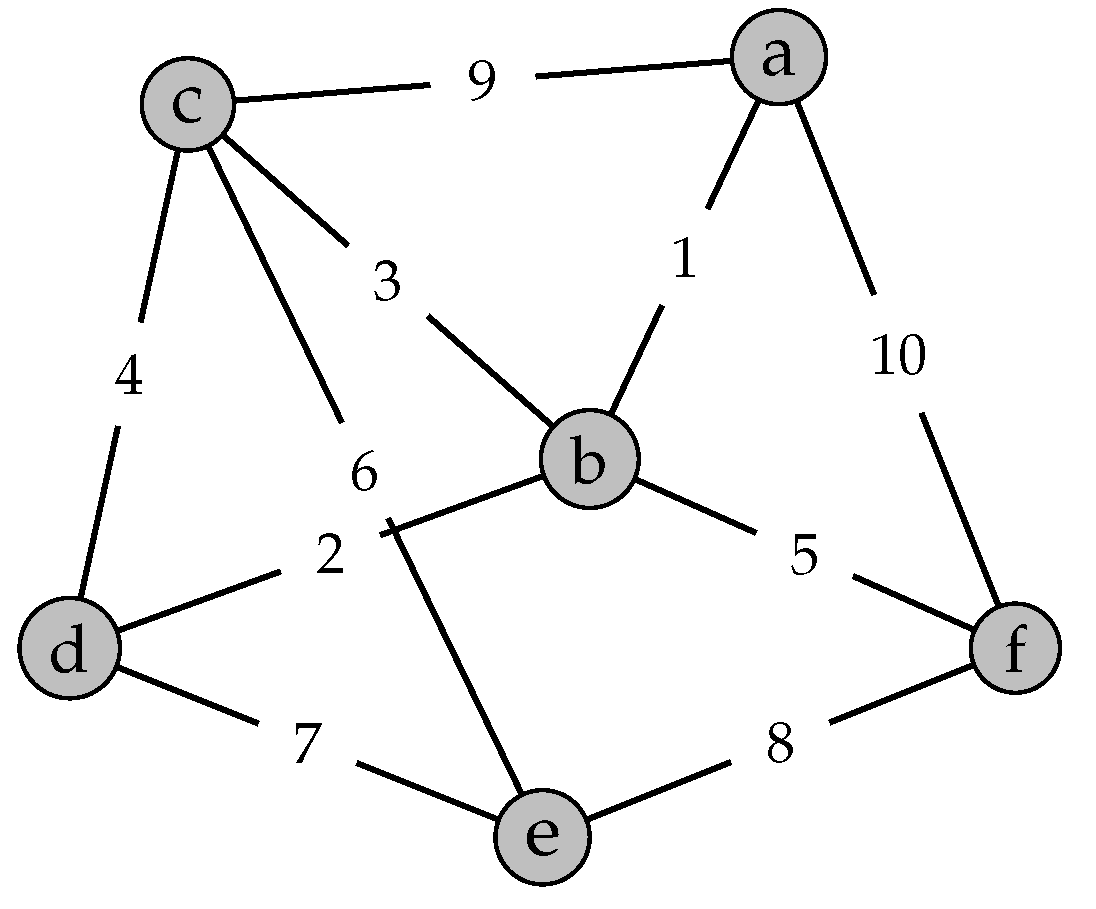
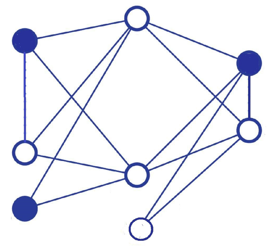
Example 1.

Consider a network that consists of six nodes and 10 links with the graph depicted in Figure 1.

The network is assumed to work if there is a connection between some of nodes which we consider them as terminals. We consider two different sets of terminals for the network:

• First, we consider all nodes as terminals, $\mathbb{T}=\mathbb{V}$ (all-terminal connectivity). In this case, we can show that the corresponding signature vector of a network is as follows:

  $$\mathbf{s}=(0,0,\frac{1}{30},\frac{9}{70},\frac{29}{90},\frac{65}{126},0,0,0,0).$$
• Second, assume that the network is working if there is a connection between nodes c and f. That is, the terminals set is ${\mathbb{T}}^{★}=\{c,f\}$. In this case, the signature vector is obtained as

  $${\mathbf{s}}^{★}=(0,0,\frac{1}{120},\frac{37}{840},\frac{179}{1260},\frac{379}{1260},\frac{19}{70},\frac{1}{6},\frac{1}{15},0).$$
  An algorithm for calculating these signatures is available from the authors upon the request.
  Assume that, in each case, the network is subjected to failure based on the GCPs with the same MVFs. Denote the lifetimes of the network corresponding to (a) and (b) by T and $T^{★}$, respectively. Comparing the corresponding survival signatures of network for two cases shows that $\overline{S_i}\le \overline{S_i^{★}}$, for $i=0,1,\cdots ,9$, and hence based on (3) we have $T{\le }_{st}{T}^{*}$ implying that the network with two-terminal connectivity is more reliable than the network with all-terminal connectivity, as expected intuitively.

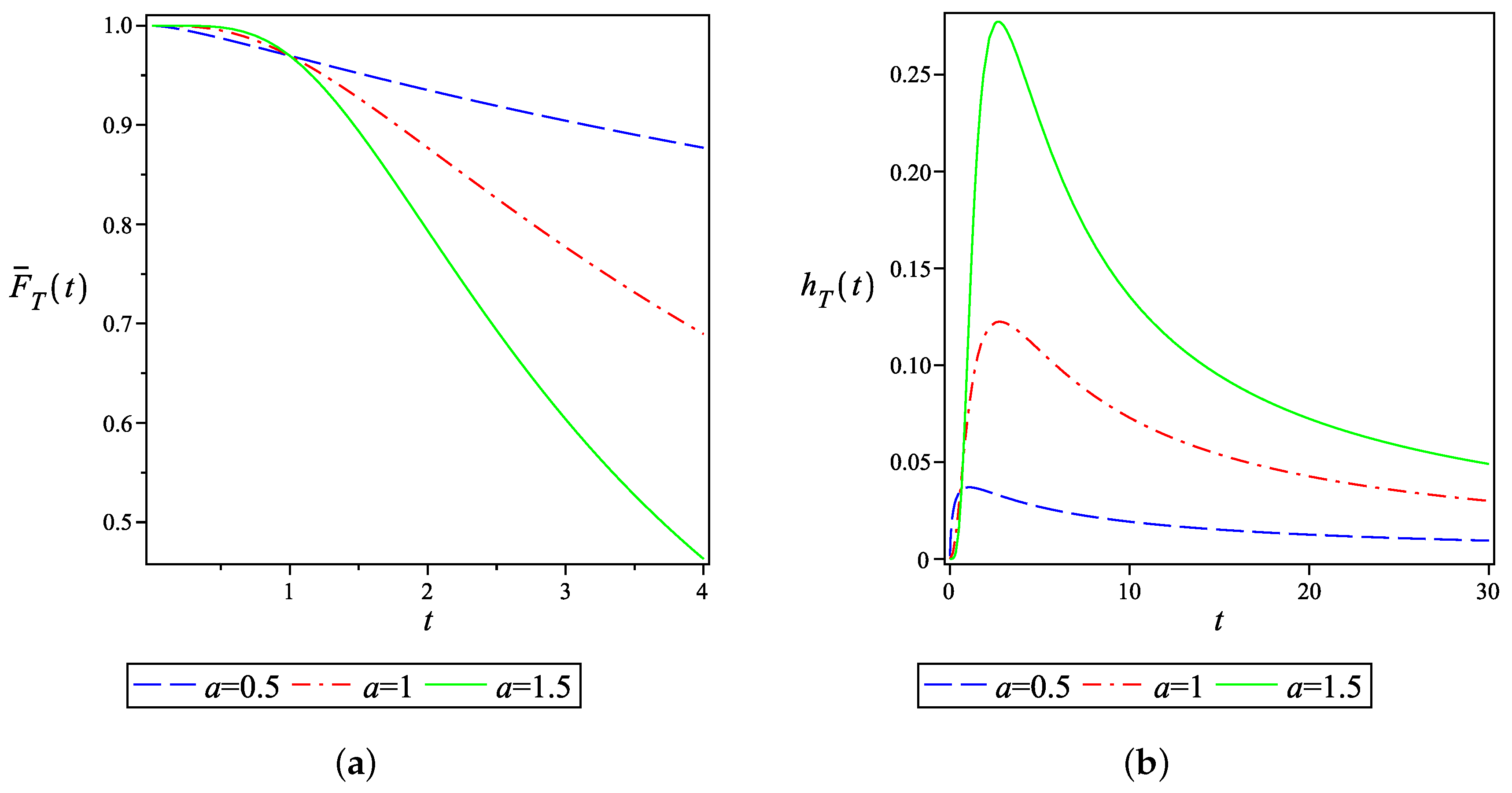
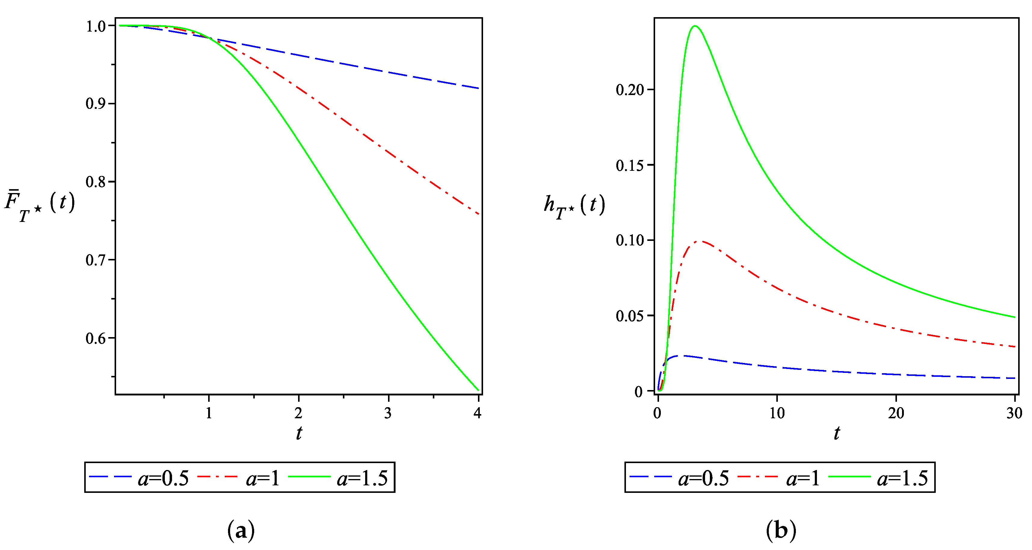
Figure 2a gives the plot of network reliability in the case of all-terminal connectivity, $\mathbb{T}=\mathbb{V}$, and when $\Lambda (t)=t^a$, for different values of a. As seen, the reliability function of network does not order with respect to a for all $t>0$. Of course, this is true in any network when MVF $\Lambda (t)=t^a$, $a>0$. This is so using the fact that

$$P({\vartheta }_k>t;a)=\left[1-{\left(\frac{t^a}{1+t^a}\right)}^k\right]$$

is increasing (decreasing) in a for $0<t<1$ ($t>1$), for a general signature vector $\mathbf{s}$ the reliability of the network

$$\begin{array}{c}\hfill P(T>t;a)=\sum _{k=1}^n{s}_{k}P({\vartheta }_k>t;a),\end{array}$$

is also increasing (decreasing) in a for $0<t<1$ ($t>1$). Figure 2b represents the hazard rate of network when $\mathbb{T}=\mathbb{V}$ for $a=0.5,1,1.5$. Figure 3a,b shows the plots of reliability function and hazard rate of the network lifetime when the terminals set is considered as ${\mathbb{T}}^{★}=\{c,f\}$.

It is interesting to compare the network reliability when the failure of components appear according to a GCP and the network reliability when the failure of components occur based on an NHPP. In the sequel, we show that, if the network has a series structure, then the reliability of the network in the GCP model dominates the reliability of the network in an NHPP model. Consider a two-state series network with the property that the first and the last components are considered to be terminals. We assume that the network fails if the linkage between the two terminals are disconnected. This occurs at the time of the first component failure. Let $T_{NP}$ and $T_{GP}$ denote the lifetimes of the network when the component failure appears according to NHPP and GCP with the same MVF $\Lambda (t)$, respectively. If ${\vartheta }_{1,NP}$ and ${\vartheta }_{1,GP}$ denote the arrival times of the first component failure based on NHPP and GCP, respectively, then, from inequality $e^x>(1+x)$, $x>0$, we can write

$$\begin{array}{c}\hfill P({\vartheta }_{1,NP}>t)=e^{-\Lambda (t)}<\frac{1}{1+\Lambda (t)}=P({\vartheta }_{1,GP}>t).\end{array}$$

Hence, based on the fact that, for a series network $\mathbf{s}=(1,0,\cdots ,0)$, relation (2) implies that $T_{NP}{\le }_{st}{T}_{GP}$.

The following example reveals that the above result, proved for the series network, is not necessarily true for any network.

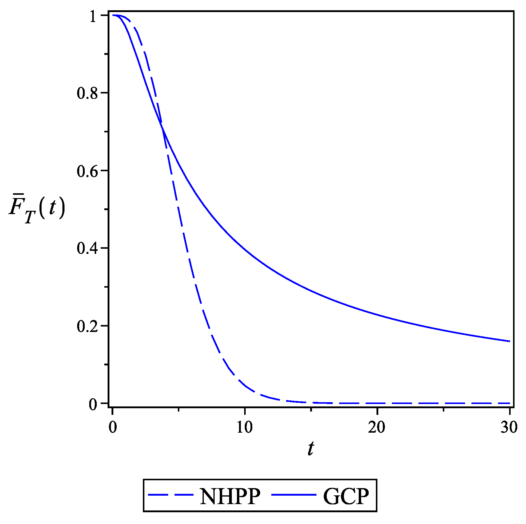
Example 2.

Consider the network described in Example 1. Figure 4 shows that the reliability functions of the network for part (a). As the plots show the reliability functions are not ordered in NHPP and GCP models with the same MVFs $\Lambda (t)=t$. The reliability of the network in the NHPP model is higher than the GCP model for the early times of operating of the network. However, when the time goes ahead, the network reliability in NHPP declines rapidly and stays below the reliability of the GCP model.

The next theorem explores the monotonicity relation of the intensity function of the process and the hazard rate of the network.

Theorem 1.

Let the components of a network fail based on a GCP with increasing intensity function $\lambda (t)$. Then, the hazard rate of network is increasing if and only if $\psi (u)$ is increasing in u where

$$\begin{array}{c}\hfill \psi (u)=\frac{{\sum }_{k=0}^{n-1}(k+1)s_{k+1}{u}^k}{{\sum }_{k=0}^{n-1}{\overline{S}}_k{u}^k}.\end{array}$$

(8)

Proof. 

From (3) and (4), the hazard rate of network can be written as

$$\begin{array}{c}\hfill h_T(t)=\frac{f_T(t)}{{\overline{F}}_T(t)}=\lambda (t)\psi (\mu (t)),\end{array}$$

(9)

where $\psi (·)$ is defined in (8) and $\mu (t)=\Lambda (t)/(1+\Lambda (t))$ is increasing in t. If $\psi (t)$ is increasing, from (9), it can be easily seen that $h_T(t)$ is increasing. This completes the ‘if’ part of the theorem. To prove ‘only if’ part of the theorem, let $h_T(t)$ be increasing and $\psi (t)$ be decreasing in the interval $(a,b)$. For MVF $\Lambda (t)=ct$, $c>0$, and hence $\lambda (t)=c$ as an increasing function, we conclude that $h_T(t)$ is decreasing on interval $(a,b)$, which contradicts with the assumption that the hazard rate of network is increasing for all t. □

Theorem 2.

Let T and $T^{★}$ denote the lifetimes of two networks with signature vectors $\mathbf{s}=(s_1,\cdots ,s_n)$ and ${\mathbf{s}}^{★}=(s_1^{★},\cdots ,s_n^{★})$, respectively. Suppose that the components of networks fail based on GCPs with MVFs $\Lambda (t)$ and ${\Lambda }^{★}(t)$, respectively. If $\mathbf{s}{\le }_{st}{\mathbf{s}}^{★}$ and $\Lambda (t)\ge {\Lambda }^{★}(t)$ for all $t\ge 0$, then $T{\le }_{st}{T}^{★}$.

Proof. 

Let ${\vartheta }_k$ and ${\vartheta }_k^{★}$ denote the kth arrival times of the two processes, $k=1,\dots ,n$. Since $P({\vartheta }_k\le {\vartheta }_{k+1})=1$, then, from Theorem 1.A.1 of [16], we can write ${\vartheta }_k{\le }_{st}{\vartheta }_{k+1}$. Hence,

$$\begin{array}{c}\hfill P(T>t)=\sum _{k=1}^n{s}_k{\overline{F}}_{{\vartheta }_k}(t)\le \sum _{k=1}^n{s}_k^{★}{\overline{F}}_{{\vartheta }_k}(t).\end{array}$$

(10)

In addition, the condition $\Lambda (t)\ge {\Lambda }^{★}(t)$ for all $t\ge 0$ implies that ${\vartheta }_k{\le }_{st}{\vartheta }_k^{★}$, $k=1,\dots ,n$. Then, we get

$$\begin{array}{c}\hfill \sum _{k=1}^n{s}_k^{★}{\overline{F}}_{{\vartheta }_k}(t)\le \sum _{k=1}^n{s}_k^{★}{\overline{F}}_{{\vartheta }_k^{★}}(t)=P(T^{★}>t).\end{array}$$

(11)

Hence, the result follows from (10) and (11). □

Theorem 3.

For two networks as described in Theorem 2, assume that the failure of components of both networks appear according to the same GCPs:

• If $\mathbf{s}{\le }_{st}{\mathbf{s}}^{★}$, then $T{\le }_{st}{T}^{★}$,
• If $\mathbf{s}{\le }_{hr}{\mathbf{s}}^{★}$, then $T{\le }_{hr}{T}^{★}$,
• If $\mathbf{s}{\le }_{rh}{\mathbf{s}}^{★}$, then $T{\le }_{rh}{T}^{★}$,
• If $\mathbf{s}{\le }_{lr}{\mathbf{s}}^{★}$, then $T{\le }_{lr}{T}^{★}$.

Proof. 

It can be easily shown that ${\vartheta }_k{\le }_{lr}{\vartheta }_{k+1}$$k=1,2,\cdots$. Since lr-ordering implies hr-, rh- and st-ordering, parts (i), (ii), (iii), and (iv) are proved, by using (2), from Theorems 1.A.6, 1.B.14, 1.B.52, and 1.C.17 of [16], respectively. □

From part (ii) of Theorem 3, since hr-ordering implies mrl-ordering, we conclude that if $\mathbf{s}{\le }_{hr}{\mathbf{s}}^{★}$ then $T{\le }_{mrl}{T}^{★}$. However, the following example shows that the assumption $\mathbf{s}{\le }_{hr}{\mathbf{s}}^{★}$ can not be replaced with $\mathbf{s}{\le }_{mrl}{\mathbf{s}}^{★}$ to have $T{\le }_{mrl}{T}^{★}$.

Example 3.

Consider two networks with signature vectors $\mathbf{s}=(0,2/3,1/3)$ and ${\mathbf{s}}^{★}=(1/3,0,2/3)$. It is easy to see that $\mathbf{s}{\le }_{mrl}{\mathbf{s}}^{★}$. However, $\mathbf{s}{\nleqq }_{st}{\mathbf{s}}^{★}$ and hence $\mathbf{s}{\nleqq }_{hr}{\mathbf{s}}^{★}$. Assume that the components of both networks fail based on the same GCPs with MVF $\Lambda (t)=t^2$. Then, a straightforward calculation gives $E(T)=2.5525>E(T^{★})=2.4871$, which, in turn, implies that $T{\nleqq }_{mrl}{T}^{★}$.

Residual Lifetime of a Working Network

Let T denote the lifetime of a network whose components are subjected to failure based on a GCP with MVF $\Lambda (t)$. If the network is up at time t, then the residual lifetime of the network is presented by the conditional RV $(T-t|T>t)$ with conditional reliability function given as

$$\begin{array}{cc}\hfill P(T-t>x|T>t)=& \frac{1}{P(T>t)}\sum _{k=1}^n{s}_{k}P({\vartheta }_k>t+x)\hfill \\ \hfill =& \sum _{k=1}^n{s}_k(t)P({\vartheta }_k-t>x|{\vartheta }_k>t),\hfill \end{array}$$

where $s_k(t)$ is the kth element of vector ${\mathbf{s}}_k(t)$ as defined in (6). This shows that the reliability function of the residual lifetime of the network is a mixture of the reliability functions of residual lifetimes of the first n arrival times of GCP, where the mixing probability vector is $\mathbf{s}(t)=(s_1(t),\dots ,s_n(t))$. As we have already mentioned, $s_k(t)$ is in fact the probability that the kth component failure causes the failure of the network, given that the lifetime of the network is more than t; that is,

$$\begin{array}{c}\hfill s_k(t)=P(T={\vartheta }_k|T>t),k=1,2,\dots ,n.\end{array}$$

In what follows, we call the vector $\mathbf{s}(t)$ as the conditional signature of the network. In the sequel, we give some stochastic properties of the conditional signature of network under the condition that the components of the network fail based on GCP model.

Theorem 4.

Consider a network with signature vector $\mathbf{s}=(s_1,s_2,\cdots ,s_n)$. With $M=max\left\{i\right|s_i>0\}$, ${lim}_{t\to 0}\mathbf{s}(t)=\mathbf{s}$ and ${lim}_{t\to \infty }\mathbf{s}(t)=\tilde{\mathbf{s}}$ where $\tilde{\mathbf{s}}=({\tilde{s}}_1,\cdots ,{\tilde{s}}_M)$ and ${\tilde{s}}_i=\frac{i{s}_i}{{\sum }_{k=1}^{n}k{s}_k}$, $i=1,\cdots ,n$.

Proof. 

From (6), we can write

$$s_i(t)={\displaystyle \frac{s_i\left[1-{(\frac{\Lambda (t)}{1+\Lambda (t)})}^i\right]}{{\sum }_{k=1}^M{s}_k\left[1-{(\frac{\Lambda (t)}{1+\Lambda (t)})}^k\right]}},i=1,\cdots ,n.$$

Then, it is easily seen that, for any i, ${lim}_{t\to 0}{s}_i(t)=s_i$ and hence

$$\underset{t\to 0}{lim}\mathbf{s}(t)=\mathbf{s}.$$

On the other hand, for $i=1,\cdots ,n$,

$$\begin{array}{cc}\hfill \underset{t\to \infty }{lim}{s}_i(t)& =\underset{u\to 1}{lim}\frac{s_i(1-u^i)}{{\sum }_{k=1}^n{s}_k(1-u^k)},\hfill \\ & =\underset{u\to 1}{lim}\frac{i{s}_i{u}^{i-1}}{{\sum }_{k=1}^{n}k{s}_k{u}^{k-1}}=\frac{i{s}_i}{{\sum }_{k=1}^{n}k{s}_k},\hfill \end{array}$$

and consequently the result follows. □

Example 4.

For the network in Example 1, with $\Lambda (t)=t^a$, we have

$$\begin{array}{c}\hfill h_{{\vartheta }_i}(t)=\frac{ak{t}^{ak}}{(1+t^a)\left[{(1+t^a)}^k-t^{ak}\right]},i=1,2,\cdots .\end{array}$$

Hence, it is easily seen that ${lim}_{t\to \infty }{h}_{{\vartheta }_i}(t)=0$. Thus, based on (5) and Theorem 4, we have ${lim}_{t\to \infty }{h}_T(t)=0$ for any network structure.

Theorem 5.

Consider a network whose components fail based on two different GCPs with MVFs $\Lambda (t)$ and ${\Lambda }^{★}(t)$, respectively. Denote by $\mathbf{s}(t)$ and ${\mathbf{s}}^{★}(t)$ the corresponding conditional signatures of the two networks. Then,

• $\mathbf{s}(t)$ and ${\mathbf{s}}^{★}(t)$ are increasing in the sense of st-ordering with respect to t;
• $\Lambda (t)\le {\Lambda }^{★}(t)$ implies that $\mathbf{s}(t){\le }_{st}{\mathbf{s}}^{★}(t)$ for all $t\ge 0$.

Proof. 

With $\delta (i,u)=1-u^i$, from (6), for each MVF $\Lambda (t)$, $s_i(t)$ can be written as

$$\begin{array}{c}\hfill s_i(t)=\frac{s_i\delta (i,\mu (\Lambda (t)))}{{\sum }_{i=1}^n{s}_i\delta (i,\mu (\Lambda (t))},i=1,\cdots ,n,\end{array}$$

(12)

where $\mu (v)=v/(1+v)$. Then, we have

$$\begin{array}{c}\hfill \sum _{i=k}^n{s}_i(t)={\beta }_k(\mu (\Lambda (t))),\end{array}$$

in which

$$\begin{array}{c}\hfill {\beta }_k(u)=\frac{{\sum }_{i=k}^n{s}_i[1-u^i]}{{\sum }_{i=1}^n{s}_i[1-u^i]}.\end{array}$$

For $i_1\le i_2$,

$$\begin{array}{cc}\hfill \frac{\delta (i_2,u)}{\delta (i_1,u)}=& \frac{1-u^{i_2}}{1-u^{i_1}}=\frac{{\sum }_{j=0}^{i_2-1}{u}^j}{{\sum }_{j=0}^{i_1-1}{u}^j}\hfill \\ \hfill =& \frac{{\sum }_{j=0}^{i_1-1}{u}^j+{\sum }_{j=i_1}^{i_2-1}{u}^j}{{\sum }_{j=0}^{i_1-1}{u}^j}\hfill \\ \hfill =& 1+\sum _{j^{\prime }=i_1}^{i_2-1}\frac{1}{{\sum }_{j=0}^{i_1-1}{u}^{j-j^{\prime }}}\hfill \end{array}$$

(13)

is increasing in u and hence $\delta (i,u)$ is TP${}_2$ in i and u. Using this fact and Lemma 2.4 of [13]:

• Since $\mu (u)$ is increasing in u, then, for an arbitrary MVF $\Lambda (·)$, we have

  $$\sum _{i=k}^n{s}_i(t)\le \sum _{i=k}^n{s}_i(t^{\prime }),t\le t^{\prime }.$$
• Since $\mu (u)$ is increasing in u, and $\Lambda (t)\le {\Lambda }^{★}(t)$ for all $t\ge 0$, then

  $$\sum _{i=k}^n{s}_i(t)\le \sum _{i=k}^n{s}_i^{★}(t),t\ge 0.$$

Therefore, the proof of the theorem is complete. □

The following lemma from [13] is useful to get some stochastic properties of conditional signature expressed in (6). Before expressing the lemma, we recall that a non-negative function $f(x)$, $x\ge 0$, is said to be upside-down bathtub-shaped if it is increasing on $[0,a]$, is constant on $[a,b]$ and is decreasing on $[b,\infty )$ where $0\le a\le b\le \infty$.

Lemma 1.

Let $\alpha (.)$ and $\beta (.)$ be non-negative discrete functions and γ be positive and real-valued. Define

$$\begin{array}{c}\hfill \tau (u)=\frac{\gamma {\sum }_{i=l^{\prime }}^{k^{\prime }}\alpha (i)u^i}{{\sum }_{i=l}^k\alpha (i)\beta (i)u^i},u>0,\end{array}$$

(14)

where $l\le l^{\prime }$, $l^{\prime }<k^{\prime }$ and $k^{\prime }\le k$. Assume that $\beta (.)$ is a non-constant decreasing (increasing) function on $\{l^{\prime },l^{\prime }+1,\dots ,k^{\prime }\}$. Then, for $l=l^{\prime }$ and $k^{\prime }<k$($k=k^{\prime }$ and $l^{\prime }>l$), we have

• $\tau (u)$ is upside-down bathtub-shaped with a single change-point;
• $\tau (u)$ is bounded above by $\gamma /\beta (k^{\prime })$$(\gamma /\beta (l^{\prime }))$.

Now, we have the following theorem.

Theorem 6.

For a network with signature vector $\mathbf{s}=(s_1,\cdots ,s_n)$,

• $s_m(t)$ is decreasing in t and $s_M(t)$ is increasing in t where $m=min\left\{i\right|s_i>0\}$ and $M=max\left\{i\right|s_i>0\}$;
• $s_j(t)$, $m\le j\le M$, is upside-down bathtub-shaped with a single change-point;
• $s_j(t)$, $m\le j\le M$, is bounded above by $s_j/{\overline{S}}_{j-1}$;
• The maximum value of $s_j(t)$, $m\le j\le M$, does not depend on the MVF $\Lambda (t)$.

Proof. 

Assume that $\mu (t)=t/(1+t)$. From (12), we can write

$$\begin{array}{c}\hfill s_m(t)=s_m{\left(\sum _{i=m}^M{s}_i\frac{\delta (i,\mu (\Lambda (t)))}{\delta (m,\mu (\Lambda (t)))}\right)}^{-1}{s}_M(t)=s_M{\left(\sum _{i=m}^M{s}_i\frac{\delta (i,\mu (\Lambda (t)))}{\delta (M,\mu (\Lambda (t)))}\right)}^{-1}.\end{array}$$

(15)

As seen in (13), $\delta (i_2,x)/\delta (i_1,x)$, for $i_2\ge i_1$, is increasing in x. Since $\mu (\Lambda (t))$ is increasing in t, then it can be concluded that $\delta (i_2,\mu (\Lambda (t)))/\delta (i_1,\mu (\Lambda (t)))$ is also increasing in t, for $i_2\ge i_1$. Based on this fact and (15), we observe that $s_m(t)$ is a decreasing function of t and $s_M(t)$ is an increasing function of t. This completes the proof of part (a).

From relation (7), we have

$$\begin{array}{c}\hfill s_j(t)=\frac{s_j{\sum }_{i=0}^{j-1}{\left(\mu (\Lambda (t))\right)}^i}{{\sum }_{i=0}^{n-1}{\overline{S}}_i{\left(\mu (\Lambda (t))\right)}^i}.\end{array}$$

With $\gamma =s_j$, $\alpha (i)=1$, $\beta (i)={\overline{S}}_i$, $l=l^{\prime }=0$, $k^{\prime }=j-1$ and $k=n-1$ in (14), define ${\omega }_j(u):=\tau (u)$. Then, we can write

$$s_j(t)={\omega }_j\left(\mu \left(\Lambda (t)\right)\right).$$

Since $\mu \left(\Lambda (t)\right)$ is increasing in t, parts (b) and (c) follow from parts (i) and (ii) of Lemma 1.

Part (d) can be proved from the fact that

$$\underset{t>0}{max}{s}_j(t)=\underset{t>0}{max}{\omega }_j\left(\mu \left(\Lambda (t)\right)\right)=\underset{t>0}{max}{\omega }_j(t).$$

 □

The following theorem compares the performance of two used networks based on their conditional signatures.

Theorem 7.

Let $\mathbf{s}(t)$ and ${\mathbf{s}}^{★}(t)$ be the conditional signatures of two networks with lifetimes T and $T^{★}$, respectively. Suppose that the component failure in both networks appear based on the same GCPs.

• If $\mathbf{s}(t){\le }_{st}{\mathbf{s}}^{★}(t),$ then $(T-t|T>t){\le }_{st}(T^{★}-t|T^{★}>t)$;
• If $\mathbf{s}(t){\le }_{hr}{\mathbf{s}}^{★}(t),$ then $(T-t|T>t){\le }_{hr}(T^{★}-t|T^{★}>t)$;
• If $\mathbf{s}(t){\le }_{rh}{\mathbf{s}}^{★}(t),$ then $(T-t|T>t){\le }_{rh}(T^{★}-t|T^{★}>t)$;
• If $\mathbf{s}(t){\le }_{lr}{\mathbf{s}}^{★}(t),$ then $(T-t|T>t){\le }_{lr}(T^{★}-t|T^{★}>t)$.

Proof. 

It can be easily seen that ${\vartheta }_k{\le }_{lr}{\vartheta }_{k+1}$, $k=1,\dots ,n-1$. Then, from Theorem 1.C.6 of [16], we have, for $k=1,\dots ,n-1$ and $t\ge 0$,

$$({\vartheta }_k-t|{\vartheta }_k>t){\le }_{lr}({\vartheta }_{k+1}-t|{\vartheta }_{k+1}>t).$$

Hence, these residual lifetimes are also hr-, rh- and st-ordered. Since $\mathbf{s}(t){\le }_{st}{\mathbf{s}}^{★}(t)$, from Theorem 1.A.6 of [16], we have, for all $x>0$,

$$\begin{array}{cc}\hfill P(T-t>x|T>t)=& \sum _{k=1}^n{s}_k(t)P({\vartheta }_k-t>x|{\vartheta }_k>t)\hfill \\ \hfill \le & \sum _{k=1}^n{s}_k^{★}(t)P({\vartheta }_k-t>x|{\vartheta }_k>t)=P(T^{★}-t>x|T^{★}>t).\hfill \end{array}$$

This establishes part (a). The proof of parts (b), (c) and (d) are obtained similarly by using Theorems 1.B.14, 1.B.52, and 1.C.17 of [16], respectively. □

3. Three-State Networks under GCP of Component Failure

In this section, we study the reliability of the lifetimes of the networks with three states under the condition that the components fail according to a GCP with MVF $\Lambda (t)=\lambda t$. In order to develop the results, we need the notion of two-dimensional signature that has been defined for single-step three-state networks by Gertsbakh and Shpungin [11]. Throughout this section, we are dealing with a single-step three-state network consisting of n binary components where we assume that the network has three states: up (denoted by $K=2$), partial performance (denoted by $K=1$) and down (denoted by $K=0$). Suppose that the network starts to operate at time $t=0$ where it is in state $K=2$. Denote by ${\mathcal{T}}_1$ the time that the network remains in state $K=2$ and by ${\mathcal{T}}_2$ the network lifetime i.e., the entrance time into state $K=0$. Let I (J) be the number of failed components when the network enters into state $K=1$ ($K=0$). Gertsbakh and Shpunging [11] introduced the notion of two-dimensional signature as

$$\begin{array}{c}\hfill s_{i,j}=P(I=i,J=j)=\frac{n_{i,j}}{n},1\le i<j\le n,\end{array}$$

(16)

where $n_{i,j}$ represents the number of permutations in which the ith and the jth components failure change the network states from $K=2$ to $K=1$ and from $K=1$ to $K=0$, respectively. We denote by matrix $\mathcal{S}$ the two-dimensional signature with elements defined in (16). In the following, we first obtain the joint reliability function of $({\mathcal{T}}_1,{\mathcal{T}}_2)$. Under the assumption that all orders of components failure are equally probable, we have

$$\begin{array}{cc}\hfill P({\mathcal{T}}_1>t_1,{\mathcal{T}}_2>t_2)=& \sum _{i=0}^n\sum _{j=i+1}^{n}P(I=i,J=j)P(\xi (t_1)<i,\xi (t_2)<j|I=i,J=j)\hfill \\ \hfill =& \sum _{i=0}^n\sum _{j=i+1}^n{s}_{i,j}P(\xi (t_1)<i,\xi (t_2)<j),\hfill \end{array}$$

in which the second equality follows from the fact that the event $\{I=i,J=j\}$ depends only on the network structure and does not depend on the mechanism of the components failure. In addition, it can be shown, by changing the order of summations, that

$$\begin{array}{c}\hfill P({\mathcal{T}}_1>t_1,{\mathcal{T}}_2>t)=\sum _{i=0}^n\sum _{j=i}^n{\overline{S}}_{i,j}P(\xi (t_1)=i,\xi (t_2)=j),\end{array}$$

(17)

where ${\overline{S}}_{i,j}={\sum }_{k=i+1}^{n-1}{\sum }_{j=max\{k,j\}+1}^n{s}_{k,l}$.

Suppose that the component failures occur at random times ${\vartheta }_1,\cdots ,{\vartheta }_n$ that are corresponding to the first n arrival times of the GCP $\{\xi (t),t\ge 0\}$. Using the fact that the event $(\xi (t)=i)$ occurs if and only if $({\vartheta }_i\le t<{\vartheta }_{i+1})$, it can be shown that

$$\begin{array}{c}\hfill P({\mathcal{T}}_1>t_1,{\mathcal{T}}_2>t_2)=\sum _{i=0}^n\sum _{j=i+1}^n{s}_{i,j}P({\vartheta }_i>t_1,{\vartheta }_j>t).\end{array}$$

(18)

Assuming that the MVF of the GCP is $\Lambda (t)=\lambda t$, Di Crescenzo and Pellerey [15] obtained the PDF of $({\vartheta }_1,\cdots ,{\vartheta }_n)$ as

$$\begin{array}{c}\hfill f_{{\vartheta }_1,\cdots ,{\vartheta }_n}(t_1,\cdots ,t_n)=\frac{n!{\lambda }^n}{{(1+\lambda t_n)}^{n+1}},0<t_1<\cdots <t_n.\end{array}$$

(19)

Using (19), the joint PDF of ${\vartheta }_i$ and ${\vartheta }_j$ is achieved as

$$\begin{array}{c}\hfill f_{{\vartheta }_i,{\vartheta }_j}(t_i,t_j)=\frac{j!{\lambda }^j}{{(1+\lambda t_j)}^{j+1}}\frac{t_i^{i-1}{(t_j-t_i)}^{j-i-1}}{(i-1)!(j-i-1)!},0<t_i<t_j.\end{array}$$

(20)

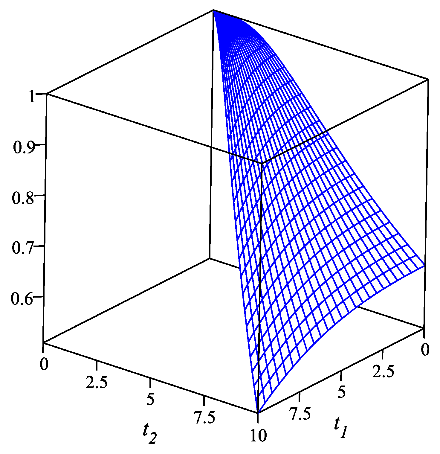
In the following, we present an example of a three-state network whose components fail according to a GCP with MVF $\Lambda (t)=\lambda t$.

Example 5.

Consider a network with a graph as depicted in Figure 5. The network has 14 links and eight nodes in which the dark nodes are considered to be terminals. Suppose that the nodes are absolutely reliable and the links are subjected to failure.

Assume that the network is in up state if all terminals are connected, in partial performance state if two terminals are connected and in down state if all terminals are disconnected. Let the network components fail according to a GCP with intensity function $\lambda (t)=1$ and all orders of links failure are equally likely. Figure 6 presents the plot of joint reliability function of the network lifetimes $({\mathcal{T}}_1,{\mathcal{T}}_2)$. The elements $s_{i;j}$ of the two-dimensional signature are calculated using an algorithm by the authors, which can be provided to the readers upon the request.

In the following theorem, we compare the state lifetimes of two three-state networks. In order to do this, we need the following Lemma.

Lemma 2.

Assume that $\{{\xi }_1(t),t\ge 0\}$ and $\{{\xi }_2(t),t\ge 0\}$ are two GCPs with intensity functions ${\lambda }_1(t)={\lambda }_1>0$, and ${\lambda }_2(t)={\lambda }_2>0$, respectively. Let ${\vartheta }_{1,1},{\vartheta }_{1,2},\cdots$ and ${\vartheta }_{2,1},{\vartheta }_{2,2},\cdots$ denote the arrival times corresponding to the two processes, respectively. If ${\lambda }_1\ge {\lambda }_2,$ then $({\vartheta }_{1,1},\cdots ,{\vartheta }_{1,n}){\le }_{st}({\vartheta }_{2,1},\cdots ,{\vartheta }_{2,n})$ for every $n\ge 1$.

Proof. 

Using relation (19), it can be seen that $f_{{\vartheta }_{i,1},\cdots ,{\vartheta }_{i,n}}$ is ${\mathrm{MTP}}_2$, which implies that ${\vartheta }_{i,1}$,..., ${\vartheta }_{i,n}$ are associated, $i=1,2$. In addition, we have

$$\begin{array}{c}\hfill \frac{f_{{\vartheta }_{2,1},\cdots ,{\vartheta }_{2,n}}(t_1,\cdots ,t_n)}{f_{{\vartheta }_{1,1},\cdots ,{\vartheta }_{1,n}}(t_1,\cdots ,t_n)}={(\frac{{\lambda }_2}{{\lambda }_1})}^n{(\frac{1+{\lambda }_1{t}_n}{1+{\lambda }_2{t}_n})}^{n+1},0<t_1<\cdots <t_n,\end{array}$$

which is increasing in $(t_1,\cdots ,t_n)$. Therefore, the required result is concluded from Theorem 6.B.8 of [16]. □

Theorem 8.

Consider two three-state networks that each consist of n components having signature matrices ${\mathcal{S}}_1$ and ${\mathcal{S}}_2$, respectively. Let the components of ith network fail according to GCP $\{{\xi }_i(t),t\ge 0\}$, $i=1,2$ with intensity function ${\Lambda }_i(t)={\lambda }_i$. Let ${\vartheta }_{i,1},{\vartheta }_{i,2},\dots$ denote the arrival times corresponding to $\{{\xi }_i(t),t\ge 0\}$. Suppose that $({\mathcal{T}}_1^{(1)},{\mathcal{T}}_2^{(1)})$ and $({\mathcal{T}}_1^{(2)},{\mathcal{T}}_2^{(2)})$ are the corresponding state lifetimes of the two networks, respectively:

• If ${\lambda }_1\ge {\lambda }_2$ and ${\mathcal{S}}_1{\le }_{uo}{\mathcal{S}}_2$, then $({\mathcal{T}}_1^{(1)},{\mathcal{T}}_2^{(1)}){\le }_{uo}({\mathcal{T}}_1^{(2)},{\mathcal{T}}_2^{(2)}),$
• If ${\lambda }_1\ge {\lambda }_2$ and ${\mathcal{S}}_1{\le }_{st}{\mathcal{S}}_2$, then $({\mathcal{T}}_1^{(1)},{\mathcal{T}}_2^{(1)}){\le }_{st}({\mathcal{T}}_1^{(2)},{\mathcal{T}}_2^{(2)}).$

Proof. 

From Lemma 2, if ${\lambda }_1\ge {\lambda }_2$, then $({\vartheta }_{1,1},\cdots ,{\vartheta }_{1,n}){\le }_{st}({\vartheta }_{2,1},\cdots ,{\vartheta }_{2,n}),$ which implies $({\vartheta }_{1,i},{\vartheta }_{1,j}){\le }_{st(uo)}({\vartheta }_{2,i},{\vartheta }_{2,j})$ for all $1\le i<j\le n$.

• Using representation (17), we have

  $$\begin{array}{cc}\hfill P({\mathcal{T}}_1^{(1)}>t_1,{\mathcal{T}}_2^{(1)}>t_2)=& \sum _{i=0}^n\sum _{j=i}^n{\overline{S}}_{1,i,j}P({\xi }_1(t_1)=i,{\xi }_1(t_2)=j)\hfill \\ \hfill \le & \sum _{i=0}^n\sum _{j=i}^n{\overline{S}}_{2,i,j}P({\xi }_1(t_1)=i,{\xi }_1(t_2)=j)\hfill \\ \hfill =& \sum _{i=0}^n\sum _{j=i+1}^n{s}_{2,i,j}P({\vartheta }_{1,i}>t_1,{\vartheta }_{1,j}>t_2)\hfill \\ \hfill \le & \sum _{i=0}^n\sum _{j=i+1}^n{s}_{2,i,j}P({\vartheta }_{2,i}>t_1,{\vartheta }_{2,j}>t_2)\hfill \\ \hfill =& P({\mathcal{T}}_1^{(2)}>t_1,{\mathcal{T}}_2^{(2)}>t_2),\hfill \end{array}$$

  where the first inequality follows from the assumption that ${\mathcal{S}}_1{\le }_{uo}{\mathcal{S}}_2$ and the second inequality follows from $({\vartheta }_{1,i},{\vartheta }_{1,j}){\le }_{uo}({\vartheta }_{2,i},{\vartheta }_{2,j})$ for $1\le i<j\le n$.
• Using the fact that $({\vartheta }_{1,i},{\vartheta }_{1,j}){\le }_{st}({\vartheta }_{2,i},{\vartheta }_{2,j})$ for all $i<j$ and the assumption that ${\mathcal{S}}_1{\le }_{st}{\mathcal{S}}_2$, the required result is concluded from Theorem 3.3 of [21].

 □

In the sequel, we investigate the dependency between ${\mathcal{T}}_1$ and ${\mathcal{T}}_2$ based on the dependency between RVs I and J. In fact, we show that, if I and J are PQD (associated), then ${\mathcal{T}}_1$ and ${\mathcal{T}}_2$ are also PQD (associated). Before that, let

$$s_i^{(1)}=P(I=i),s_j^{(2)}=P(J=j),$$

and ${\overline{S}}_i^{(k)}={\sum }_{l=i+1}^n{s}_l^{(k)},k=1,2$.

Theorem 9.

Let ${\mathcal{T}}_1$ be the lifetime of a three-state network in state $K=2$ and ${\mathcal{T}}_2$ be the lifetime of the network. Let the components failure of the network appear according to the GCP $\{\xi (t),t\ge 0\}$ with arrival times ${\vartheta }_1,\cdots ,{\vartheta }_n$.

• If I and J are PQD, then ${\mathcal{T}}_1$ and ${\mathcal{T}}_2$ are PQD.
• If I and J are associated, then ${\mathcal{T}}_1$ and ${\mathcal{T}}_2$ are associated.

Proof. 

From representation (20), one can show that $f_{{\vartheta }_i,{\vartheta }_j}(t_i,t_j)$ is ${\mathrm{TP}}_2$, which implies that ${\vartheta }_i$ and ${\vartheta }_j$ are associated and PQD.

(a)

Let $\varphi (·)$ and $\psi (·)$ be two increasing functions. From representation (18), we have

$$\begin{array}{cc}\hfill E(\varphi ({\mathcal{T}}_1)\psi ({\mathcal{T}}_2))=& \sum _{i=1}^{n-1}\sum _{j=i+1}^n{s}_{i,j}E(\varphi ({\vartheta }_i)\psi ({\vartheta }_j))\hfill \\ \hfill \ge & \sum _{i=1}^{n-1}\sum _{j=i+1}^n{s}_{i,j}E(\varphi ({\vartheta }_i))E(\psi ({\vartheta }_j))\hfill \\ \hfill \ge & \sum _{i=1}^n{s}_i^{(1)}E(\varphi ({\vartheta }_i))\sum _{j=1}^n{s}_j^{(2)}E(\psi ({\vartheta }_j))\hfill \\ \hfill =& E(\varphi ({\mathcal{T}}_1))E(\psi ({\mathcal{T}}_2)),\hfill \end{array}$$

where the first inequality follows from the fact that ${\vartheta }_i$ and ${\vartheta }_j$ are PQD and the second inequality follows from the assumption that I and J are PQD.

(b)

Proof of part (b) is the same as the proof of part (a) using the fact that, for every two-variate increasing functions ${\varphi }^{\prime }(·,·)$ and ${\psi }^{\prime }(·,·)$,

$$\begin{array}{c}\hfill E({\varphi }^{\prime }({\mathcal{T}}_1,{\mathcal{T}}_2){\psi }^{\prime }({\mathcal{T}}_1,{\mathcal{T}}_2))=\sum _{i=1}^{n-1}\sum _{j=i+1}^n{s}_{i,j}E({\varphi }^{\prime }({\vartheta }_i,{\vartheta }_j){\psi }^{\prime }({\vartheta }_i,{\vartheta }_j)).\end{array}$$

 □

The results of the theorem are interesting in the sense that the PQD (associated) property of I and J, which is non-aging and depends only on the structure of the network, is transferred to the PQD (associated) property of ${\mathcal{T}}_1$ and ${\mathcal{T}}_2$, which is the aging characteristic of the network.

Example 6.

Consider again the network presented in Example 5. It can be seen that, for every $i,j=1,\cdots ,14$, ${\overline{S}}_{i,j}\ge {\overline{S}}_i^{(1)}{\overline{S}}_j^{(2)}$. This implies that I and J are PQD. Hence, if the components fail according to a GCP, then ${\mathcal{T}}_1$ and ${\mathcal{T}}_2$ are PQD.

4. Conclusions

In this article, we studied the reliability, aging and stochastic characteristics of an n-component network whose components were subjected to failure according to a geometric counting process (GCP). We first considered the case that the network has two states (up and down). Some mixture representations of the network reliability were obtained in terms of signature of the network and the reliability functions of the arrival times of the GCP. We studied the conditions under which the hazard rate of the network is increasing in the case that intensity function of the process is increasing. Stochastic comparisons were made between the lifetimes of different networks, subjected to GCPs, based on the stochastic comparisons between their signatures. The residual lifetime of the network was also explored. In the second part of the paper, we considered the networks with three states: up, partial performance, and down. The components of the network were assumed to fail based on a GCP with mean value function $\Lambda (t)=\lambda t$, which leads to the change of the network states. Under these circumstances, we arrived at several stochastic and dependency properties of the networks with the same and different structures. The results of Section 3 were obtained under the special case that the MVF of the GCP is $\Lambda (t)=\lambda t$. The developments of the paper were mainly dependent on the notions of signature and two-dimensional signature. The results of the paper were illustrated by several examples.