A Noisy Fractional Brownian Motion Model for Multiscale Correlation Analysis of High-Frequency Prices

Abstract

We analyze the multiscale behaviors of high-frequency intraday prices, with a focus on how asset prices are correlated over different timescales. The multiscale approach proposed in this paper is designed for the analysis of high-frequency intraday prices. It incorporates microstructure noise into the stochastic price process. We consider a noisy fractional Brownian motion model and illustrate its various statistical properties. This leads us to introduce new latent correlation and noise estimators. New numerical algorithms are developed for model estimation using empirical high-frequency data. For a collection of stocks and exchange-traded funds, examples are provided to illustrate the relationship between multiscale correlation and sampling frequency as well as the evolution of multiscale correlation over time.

1. Introduction

The modern financial securities markets are populated with a wide array of market players, such as hedge funds, high-frequency firms, and other institutional and retail traders, who execute trades at various timescales, from several milliseconds to multiple days. Therefore, asset prices are driven by multiscale forces. Depending on the timescales, their price patterns may be quite different. These observations lead us to examine the multiscale properties of financial time series.

The original Brownian motion stock model by [1] intrinsically determines return distribution at any timescale as a result of independent increments and memory-less properties. Fractional Brownian motion has been proposed to challenge the efficient market hypothesis (EMH) and replace the standard Brownian motion model for asset prices (see [2,3]). It leads to a much wider class of stochastic processes with additional scaling and long-memory properties, and also allows for arbitrage opportunities, as pointed out by [4]. Fractional Brownian motion has become an important tool in financial modeling with various applications (see [5,6], among others).

As high-frequency data become increasingly available, more sophisticated models are needed to capture their dynamics. Multiscale models designed for low-frequency daily data, such as those by [7,8,9], can hardly fit the complex structure of high-frequency data, especially for (co)variance modeling (see [10,11]). It also leads to a host of new research problems, ranging from stochastic models for intraday prices and their estimations to price dependency and portfolio management implications (see, e.g., [12]).

Various approaches have been proposed to analyze the complex structure of high-frequency prices, especially their realized volatility (see, for example, [10,13]). Nevertheless, market microstructure research by [14,15], among others, suggests that there is noise at a higher frequency. As a consequence, the market microstructure noise can potentially bias estimation of the scaling parameters. For example, as shown by [16], the discrepancy between realized and instantaneous volatility can lead to bias in the estimation of the Hurst exponent ([17]). A common idea in various approaches is to conduct measurement at multiple timescales, and then, assimilate the outputs to arrive at an estimate (see [11,18,19,20,21]).

In our companion paper [22], we investigate the theoretical and empirical properties of multiscale volatility of high-frequency data. Using a fractional Brownian motion model, we estimate the Hurst exponent and noise level and illustrate the time-varying intraday patterns. In this paper, we investigate the connections between correlations and timescales of high-frequency prices. In addition, we incorporate market microstructure noise into our model to better understand how noise can affect the multiscale behaviors and associated statistical properties of correlations. This also allows us to estimate the microstructure noise realized at different times of the day, or compare the noise levels among various traded assets.

Our study begins with the definitions of multiscale correlation and some important properties in several stochastic models. In order to model high-frequency price processes, a class of multivariate noisy fractional Brownian motion models is introduced. Our analysis on multiscale correlation leads us to an equation that connects correlation and frequency. Moreover, the effect of microstructure noise is expressed analytically and examined empirically. Using intraday high-frequency price data, we illustrate the estimated correlation–frequency relationship and microstructure noise level for a collection of ETFs and stocks.

We present the definition and properties of multiscale covariance and correlation in Section 2. A fractional Brownian motion model with microstructure noise is introduced in Section 3. This leads to an analysis of the asymptotic behaviors and timescale dependence of multiscale correlation. Several illustrative examples are provided to show the correlation structures over different timescales. In Section 4, the model is estimated using empirical data. We conclude the paper in Section 5.

2. Multiscale Correlation

We consider a collection of p financial assets whose prices at time t are denoted by the vector ${\overrightarrow{P}}_t\in {\mathbb{R}}^p$. Converting to log prices ${\overrightarrow{X}}_t:=log({\overrightarrow{P}}_t)$, the log return vector over the time interval from t to $t+\tau$ is given by

$${\overrightarrow{r}}_{t,\tau }^X={\overrightarrow{X}}_{t+\tau }-{\overrightarrow{X}}_t.$$

(1)

All operations are applied element-wise. The multiscale covariance matrix can be defined as

$$\mathcal{V}[\overrightarrow{X}]\left[\tau \right]:=\mathbb{E}[({\overrightarrow{r}}_{t,\tau }^X-\mathbb{E}[{\overrightarrow{r}}_{t,\tau }^X]){({\overrightarrow{r}}_{t,\tau }^X-\mathbb{E}[{\overrightarrow{r}}_{t,\tau }^X])}^T].$$

(2)

We remark that if ${\overrightarrow{X}}_t\in {\mathbb{R}}^p$ is a stationary multivariate process, then $\mathcal{V}[\overrightarrow{X}]\left[\tau \right]\in {\mathbb{R}}^{p\times p}$ must be a matrix dependent on the time increment $\tau$ only at any time t. Next, we define the notions of multiscale pair-wise covariance and correlation.

2.1. Definition and Properties

Definition 1. 

Let the pair of log prices $X_t\in \mathbb{R}$ and $Y_t\in \mathbb{R}$ be stationary processes on $0\le t\le T$. For $\tau >0$, the multiscale covariance between X and Y is defined as

$$\mathcal{C}[X,Y]\left(\tau \right):=\mathbb{E}\left[r_{t,\tau }^X{r}_{t,\tau }^Y\right]-\mathbb{E}\left[r_{t,\tau }^X\right]·\mathbb{E}\left[r_{t,\tau }^Y\right].$$

(3)

In turn, their multiscale correlation is defined as

$$\mathcal{R}[X,Y]\left(\tau \right):=\frac{\mathcal{C}[X,Y]\left(\tau \right)}{\sqrt{\mathcal{V}\left[X\right]\left(\tau \right)·\mathcal{V}\left[Y\right]\left(\tau \right)}}.$$

(4)

Although there is no restriction on the form of the $\mathcal{R}[X,Y]\left(\tau \right)$ function, the multiscale correlation behavior is limited for a wide class of processes.

Proposition 1 

(uncorrelated increments). For any pair of stationary random processes $X_t,Y_t$ has jointly uncorrelated increments, i.e.,

$$\begin{array}{cc}\hfill \mathbb{E}\left[(X_{t_2}-X_{t_1})(X_{t_3}-X_{t_2})\right]& =\mathbb{E}[X_{t_2}-X_{t_1}]·\mathbb{E}[X_{t_3}-X_{t_2}],\hfill \\ \hfill \mathbb{E}\left[(Y_{t_2}-Y_{t_1})(Y_{t_3}-Y_{t_2})\right]& =\mathbb{E}[Y_{t_2}-Y_{t_1}]·\mathbb{E}[Y_{t_3}-Y_{t_2}],\hfill \\ \hfill \mathbb{E}\left[(X_{t_2}-X_{t_1})(Y_{t_3}-Y_{t_2})\right]& =\mathbb{E}[X_{t_2}-X_{t_1}]·\mathbb{E}[Y_{t_3}-Y_{t_2}],\hfill \\ \hfill \mathbb{E}\left[(Y_{t_2}-Y_{t_1})(X_{t_3}-X_{t_2})\right]& =\mathbb{E}[Y_{t_2}-Y_{t_1}]·\mathbb{E}[X_{t_3}-X_{t_2}],\hfill \end{array}$$

For any $0\le t_1<t_2<t_3$, the correlation function $\mathcal{R}[X,Y]\left(\tau \right)$ must be a constant in τ.

Proof. 

We first show that the covariance $\mathcal{C}[X,Y]\left(\tau \right)$ scales linearly with $\tau$:

$$\mathcal{C}[X,Y]\left(\tau \right)\propto \tau .$$

For any ${\tau }_1,{\tau }_2>0$; let us show the additive-ness $\mathcal{C}[X,Y]({\tau }_1+{\tau }_2)=\mathcal{C}[X,Y]\left({\tau }_1\right)+\mathcal{C}[X,Y]\left({\tau }_2\right)$. Consider that $0<{\tau }_1<{\tau }_1+{\tau }_2$; then,

$$\begin{array}{cc}\hfill \mathcal{C}[X,Y]({\tau }_1+{\tau }_2)& =\mathbb{E}\left[(X_{{\tau }_1+{\tau }_2}-X_0)(Y_{{\tau }_1+{\tau }_2}-Y_0)\right]-\mathbb{E}[X_{{\tau }_1+{\tau }_2}-X_0]·\mathbb{E}[Y_{{\tau }_1+{\tau }_2}-Y_0]\hfill \\ \hfill & =\mathbb{E}[((X_{{\tau }_1+{\tau }_2}-X_{{\tau }_1})+(X_{{\tau }_1}-X_0))·((Y_{{\tau }_1+{\tau }_2}-Y_{{\tau }_1})+(Y_{{\tau }_1}-Y_0))]\hfill \\ \hfill & -\mathbb{E}[(X_{{\tau }_1+{\tau }_2}-X_{{\tau }_1})+(X_{{\tau }_1}-X_0)]·\mathbb{E}[(Y_{{\tau }_1+{\tau }_2}-Y_{{\tau }_1})+(Y_{{\tau }_1}-Y_0)]\hfill \\ \hfill & =\mathbb{E}\left[(X_{{\tau }_1+{\tau }_2}-X_{{\tau }_1})(Y_{{\tau }_1+{\tau }_2}-Y_{{\tau }_1})\right]+\mathbb{E}\left[(X_{{\tau }_1}-X_0)(Y_{{\tau }_1}-Y_0)\right)]\hfill \\ \hfill & -\mathbb{E}[X_{{\tau }_1+{\tau }_2}-X_{{\tau }_1}]·\mathbb{E}[Y_{{\tau }_1+{\tau }_2}-Y_{{\tau }_1}]-\mathbb{E}[X_{{\tau }_1}-X_0]·\mathbb{E}[Y_{{\tau }_1}-Y_0]+0\hfill \\ \hfill & =\mathcal{C}[X,Y]\left({\tau }_2\right)+\mathcal{C}[X,Y]\left({\tau }_1\right).\hfill \end{array}$$

Then, $\mathcal{C}[X,Y]\left(\tau \right)\propto \tau$. Following the same derivation, the multiscale variance of the two processes also satisfies $\mathcal{V}\left[X\right]\propto \tau$ and $\mathcal{V}\left[Y\right]\propto \tau$. Therefore, the correlation must remain a fixed constant for all values of $\tau$:

$$\begin{array}{c}\hfill \mathcal{R}[X,Y]\left(\tau \right)\propto \frac{\tau }{\sqrt{\tau ·\tau }}=const.\end{array}$$

□

This means that, for the stationary processes in Proposition 1, the mulstiscale correlation stays the same at any time scale over which the correlation is computed.

Example 1 

(stochastic volatility model). Let $B_t$ and $W_t$ be independent standard Brownian motions. For $\rho \in [-1,1]$ and ${\rho }_{\sigma }\in [-1,1]$, define the following pair of correlated stochastic processes:

$$\begin{array}{cc}\hfill d{X}_t^{\left(1\right)}& ={\mu }_{1}dt+\sqrt{{\nu }_t^{\left(1\right)}}d{B}_t^{\left(1\right)},\hfill \\ \hfill d{X}_t^{\left(2\right)}& ={\mu }_{2}dt+\sqrt{{\nu }_t^{\left(2\right)}}\left(\rho d{B}_t^{\left(1\right)}+\sqrt{1-{\rho }^2}d{B}_t^{\left(2\right)}\right),\hfill \end{array}$$

where the volatility processes are

$$\begin{array}{cc}\hfill {\nu }_t^{\left(1\right)}& ={\alpha }_t^{\left(1\right)}dt+{\beta }_t^{\left(1\right)}d{W}_t^{\left(1\right)},\hfill \\ \hfill {\nu }_t^{\left(2\right)}& ={\alpha }_t^{\left(2\right)}dt+{\beta }_t^{\left(2\right)}\left({\rho }_{\sigma }d{W}_t^{\left(1\right)}+\sqrt{1-{\rho }_{\sigma }^2}d{W}_t^{\left(2\right)}\right).\hfill \end{array}$$

In the stochastic volatility model above, $B_t^{\left(1\right)},B_t^{\left(2\right)},W_t^{\left(1\right)}$, and $W_t^{\left(2\right)}$ are independent Brownian motions. The processes $(X_t^{\left(1\right)},X_t^{\left(2\right)})$ are correlated through a shared Brownian motion, so they do not have independent increments. Nevertheless, their increments are jointly uncorrelated given that

$$\mathbb{E}\left[\left({\int }_{t_1}^{t_2}\sqrt{{\nu }_t^{\left(k\right)}}d{B}_t^{\left(i\right)}\right)\left({\int }_{t_2}^{t_3}\sqrt{{\nu }_t^{\left(l\right)}}d{B}_t^{\left(j\right)}\right)\right]=0,$$

for any $i,j,k,l\in \{1,2\}$. Therefore, the correlation between $X_t^{\left(1\right)}$ and $X_t^{\left(2\right)}$ is scale-independent.

Proposition 2. 

Let $X_t^{\left(1\right)},\cdots ,X_t^{\left(n\right)}$ be a sequence of independent processes, and $Y_t^{\left(1\right)},\cdots ,Y_t^{\left(n\right)}$ be another sequence of independent processes. Further, assume that $X^{\left(i\right)}\perp Y^{\left(j\right)},\forall i\ne j$. Denote the sequence summations by $S_X={\sum }_{i=1}^n{X}^{\left(i\right)}$ and $S_Y={\sum }_{i=1}^n{Y}^{\left(i\right)}.$ Then, the multiscale correlation between the summation of the two sequences is given by

$$\mathcal{R}[S_X,S_Y]\left(\tau \right)=\sum _{i=1}^n\mathcal{R}[X^{\left(i\right)},Y^{\left(i\right)}]\left(\tau \right)·\frac{\sqrt{\mathcal{V}\left[X^{\left(i\right)}\right]\left(\tau \right)·\mathcal{V}\left[Y^{\left(i\right)}\right]\left(\tau \right)}}{\sqrt{\left({\sum }_{j=1}^n\mathcal{V}\left[X^{\left(j\right)}\right]\left(\tau \right)\right)·\left({\sum }_{j=1}^n\mathcal{V}\left[Y^{\left(j\right)}\right]\left(\tau \right)\right)}}.$$

(5)

Proof. 

Direct computation of the covariance yields the covariance

$$\begin{array}{cc}\hfill \mathcal{C}[S_X,S_Y]\left(\tau \right)& =\mathbb{E}\left[\left(\sum _{i=1}^n{r}_{t,\tau }^{X^{\left(i\right)}}\right)\left(\sum _{i=1}^n{r}_{t,\tau }^{Y^{\left(i\right)}}\right)\right]-\mathbb{E}\left[\sum _{i=1}^n{r}_{t,\tau }^{X^{\left(i\right)}}\right]\mathbb{E}\left[\sum _{i=1}^n{r}_{t,\tau }^{Y^{\left(i\right)}}\right]\hfill \\ \hfill & =\sum _{i=1}^n\mathbb{E}\left[r_{t,\tau }^{X^{\left(i\right)}}{r}_{t,\tau }^{Y^{\left(i\right)}}\right]+\sum _{i\ne j}^n\mathbb{E}\left[r_{t,\tau }^{X^{\left(i\right)}}{r}_{t,\tau }^{Y^{\left(j\right)}}\right]-\sum _{i=1}^n\mathbb{E}\left[r_{t,\tau }^{X^{\left(i\right)}}\right]\mathbb{E}\left[r_{t,\tau }^{Y^{\left(i\right)}}\right]-\sum _{i\ne j}^n\mathbb{E}\left[r_{t,\tau }^{X^{\left(i\right)}}\right]\mathbb{E}\left[r_{t,\tau }^{Y^{\left(j\right)}}\right]\hfill \\ \hfill & =\sum _{i=1}^n\mathcal{C}[X^{\left(i\right)},Y^{\left(i\right)}]\left(\tau \right)+0\hfill \\ \hfill & =\sum _{i=1}^n\mathcal{R}[X^{\left(i\right)},Y^{\left(i\right)}]\left(\tau \right)·\sqrt{\mathcal{V}\left[X^{\left(i\right)}\right]\left(\tau \right)·\mathcal{V}\left[Y^{\left(i\right)}\right]\left(\tau \right)}.\hfill \end{array}$$

The variance terms in the denominator of (5) follow from the independence of ${\left(X^{\left(i\right)}\right)}_{1=1,\dots ,n}$ and ${\left(Y^{\left(i\right)}\right)}_{1=1,\dots ,n}$. □

Remark 1. 

Note that in Equation (5), even if $\mathcal{R}[X^{\left(i\right)},Y^{\left(i\right)}]\left(\tau \right)$ is constant for all $i=1,\cdots ,n$, the correlation of the two summations can still be scale-dependent if the variance scaling behavior is different among the pairs $(X^{\left(i\right)},Y^{\left(i\right)}),i=1,\cdots ,n$.

2.2. Numerical Estimation

In order to estimate the multiscale correlation function from discrete observations, we consider a given pair of time series, $(X_i,Y_i)$, for $i=1,\cdots ,n$. The multiscale correlation can be estimated as follows.

For $m=1,2,\cdots ,M$:

• Compute variance $V_{X,m},V_{Y,m}$ using

  $$\begin{array}{cc}\hfill V_{X,m}& =\frac{1}{n-m}\sum _{i=1}^{n-m}{(X_{i+m}-X_i-{\mu }_{X}m)}^2,\hfill \\ \hfill V_{Y,m}& =\frac{1}{n-m}\sum _{i=1}^{n-m}{(Y_{i+m}-Y_i-{\mu }_{Y}m)}^2,\hfill \end{array}$$

  where

  $${\mu }_X=\frac{X_n-X_1}{n-1},\mathrm{and}{\mu }_Y=\frac{Y_n-Y_1}{n-1}$$

  are estimated drifts.
• Compute covariance:

  $$C_{XY,m}=\frac{1}{n-m}\sum _{i=1}^{n-m}(X_{i+m}-X_i-{\mu }_{X}m)(Y_{i+m}-Y_i-{\mu }_{Y}m).$$
• Compute correlation:

  $$R_{XY,m}=\frac{C_{XY,m}}{\sqrt{V_{X,m}·V_{Y,m}}}.$$

  (6)

We will apply these expressions in the sections below.

3. Multivariate High-Frequency Models

In this section, we discuss multiscale volatility in the intraday setting with high-frequency prices. The definitions of fractional Brownian motions are based on the seminal work of [3]. Then, we incorporate additional elements into the fractional Brownian motion model to create interesting scaling behaviors.

3.1. Correlated Fractional Brownian Motions

Definition 2. 

A fractional Brownian motion (fBm) $B_t^H,t\ge 0$, is a continuous-time Gaussian process that satisfies $\mathbb{E}\left[B_t^H\right]=0,\forall t\ge 0$, and has the following covariance function:

$$\mathbb{E}\left[B_t^H{B}_s^H\right]=\frac{1}{2}(t^{2H}+s^{2H}{-|t-s|}^{2H}),$$

where $t,s\ge 0$, and $H\in (0,1)$ is called the Hurst exponent.

As is well know, in the case of $H=\frac{1}{2}$, we obtain the standard Brownian motion. When $H\in (0,1/2)$, the fractional Brownian motion is called anti-persistent or mean-reverting, and its increments are negatively correlated. When $H\in (1/2,1)$, the fBm has positively correlated increments and is called persistent or trending.

A fractional Brownian motion adopts various forms of stochastic integral representation, which can be found in Chapter 1.2 of [23] and references therein. In this study, we focus on the following representation to construct a fractional Brownian motion from an underlying standard Brownian motion:

$$B_t^H=\mathcal{B}{(W;H)}_t:=\frac{1}{\Gamma (H+1/2)}{\int }_{-\infty }^t\left({(t-s)}^{H-1/2}-{(-s)}_{+}^{H-1/2}\right)d{W}_s,$$

(7)

where ${\left(W_t\right)}_{t\in \mathbb{R}}$ is the underlying Brownian motion. We will apply this representation to define correlated fractional Brownian motions and generate sample paths of fractional Brownian motions.

The correlation between Brownian motions has been well established for a long time. Like any random walk with stationary and independent increments, Brownian motion also has scale-independent correlation, as shown in Proposition 1. The correlation between fractional Brownian motions was studied more recently in the setting of multivariate fractional Brownian motion (mfBm) [24,25,26,27]. To begin with, let us first define a pair of correlated fractional Brownian motions using Equation (7) and study their correlation property.

Proposition 3. 

For any Hurst exponent pair $H_1,H_2\in (0,1)$, and for any correlation coefficient $\rho \in [-1,1]$, define the following pair of correlated fractional Brownian motions:

$$\begin{array}{cc}\hfill B_t^{H_1}& =\mathcal{B}{(W^{\left(1\right)};H_1)}_t,\hfill \\ \hfill B_t^{H_2}& =\mathcal{B}{(\rho W^{\left(1\right)}+\sqrt{1-{\rho }^2}{W}^{\left(2\right)};H_2)}_t,\hfill \end{array}$$

where $W^{\left(1\right)}$ and $W^{\left(2\right)}$ are independent standard Brownian motions, and the $\mathcal{B}(·)$ operator is defined in Equation (7). Then their multiscale correlation function is as follows:

$$\mathcal{R}[B^{H_1},B^{H_2}]\left(\tau \right)=\rho .$$

Proof. 

Without loss of generality, let us take $t=0$ in Equation (3) and analyze the increments from 0 to $\tau$. The covariance between $B^{H_1}$ and $B^{H_2}$ is

$$\begin{array}{cc}\hfill \mathcal{C}[B^{H_1},B^{H_2}]\left(\tau \right)& =\mathbb{E}\left[B_{\tau }^{H_1}{B}_{\tau }^{H_2}\right]-\mathbb{E}\left[B_{\tau }^{H_1}\right]·\mathbb{E}\left[B_{\tau }^{H_2}\right]\hfill \\ \hfill & =\mathbb{E}[\mathcal{B}{(W^{\left(1\right)};H_1)}_{\tau }·\mathcal{B}{(\rho W^{\left(1\right)}+\sqrt{1-{\rho }^2}{W}^{\left(2\right)};H_2)}_{\tau }]-0\hfill \\ \hfill & =\rho ·\mathbb{E}[\mathcal{B}{(W^{\left(1\right)};H_1)}_{\tau }·\mathcal{B}{(W^{\left(1\right)};H_2)}_{\tau }]+\sqrt{1-{\rho }^2}·\mathbb{E}[\mathcal{B}{(W^{\left(1\right)};H_1)}_{\tau }·\mathcal{B}{(W^{\left(2\right)};H_2)}_{\tau }]\hfill \\ \hfill & =\rho ·\mathbb{E}[\mathcal{B}{(W^{\left(1\right)};H_1)}_{\tau }·\mathcal{B}{(W^{\left(1\right)};H_2)}_{\tau }].\hfill \end{array}$$

Note that we have used linearity of the $\mathcal{B}(·)$ operator. To compute the expectation of the product of two stochastic integrals, we apply the generalized Ito isometry to obtain

$$\begin{array}{cc}\hfill & \mathbb{E}\left[\left({\int }_{-\infty }^{\tau }\left({(\tau -s)}^{H_1-1/2}-{(-s)}_{+}^{H_1-1/2}\right)d{W}_s\right)\left({\int }_{-\infty }^{\tau }\left({(\tau -s)}^{H_2-1/2}-{(-s)}_{+}^{H_2-1/2}\right)d{W}_s\right)\right]\hfill \\ \hfill =& {\int }_{-\infty }^{\tau }\left({(\tau -s)}^{H_1-1/2}-{(-s)}_{+}^{H_1-1/2}\right)\left({(\tau -s)}^{H_2-1/2}-{(-s)}_{+}^{H_2-1/2}\right)ds.\hfill \end{array}$$

Using a change in variable $u:=s/\tau$, we can write

$$\begin{array}{cc}\hfill & {\int }_{-\infty }^{\tau }\left({(\tau -s)}^{H1-1/2}-{(-s)}_{+}^{H_1-1/2}\right)\left({(\tau -s)}^{H_2-1/2}-{(-s)}_{+}^{H_2-1/2}\right)ds\hfill \\ \hfill =& {\int }_{-\infty }^1{\tau }^{H_1-1/2}\left({(1-u)}^{H_1-1/2}-{(-u)}_{+}^{H_1-1/2}\right){\tau }^{H_2-1/2}\left({(1-u)}^{H_2-1/2}-{(-u)}_{+}^{H_2-1/2}\right)\tau du\hfill \\ \hfill =& {\tau }^{H_1+H_2}·I(H_1,H_2),\hfill \end{array}$$

where $I(H_1,H_2)$ is the integral

$$I(H_1,H_2):={\int }_{-\infty }^1\left({(1-u)}^{H_1-1/2}-{(-u)}_{+}^{H_1-1/2}\right)\left({(1-u)}^{H_2-1/2}-{(-u)}_{+}^{H_2-1/2}\right)du.$$

In turn, we obtain the covariance

$$\begin{array}{cc}\hfill \mathcal{C}[B^{H_1},B^{H_2}]\left(\tau \right)& =\rho {\tau }^{H_1+H_2}·\frac{I(H_1,H_2)}{\Gamma (H_1+1/2)·\Gamma (H_2+1/2)}\hfill \\ \hfill & =\rho {\tau }^{H_1+H_2}.\hfill \end{array}$$

Here, we refer to [28] for canceling the integral $I(H_1,H_2)$ with the normalizing factor. The variance terms can be verified by taking $H_1=H_2$:

$$\begin{array}{cc}\hfill \mathcal{V}\left[B^{H_1}\right]\left(\tau \right)& =\mathbb{E}\left[\mathcal{B}{(W^{\left(1\right)};H_1)}_{\tau }^2\right]={\tau }^{2H_1},\hfill \\ \hfill \mathcal{V}\left[B^{H_2}\right]\left(\tau \right)& =\mathbb{E}\left[\mathcal{B}{(\rho W^{\left(1\right)}+\sqrt{1-{\rho }^2}{W}^{\left(2\right)};H_2)}_{\tau }^2\right]={\tau }^{2H_2}.\hfill \end{array}$$

And by the definition of correlation,

$$\mathcal{R}[B^{H_1},B^{H_2}]\left(\tau \right)=\rho .$$

□

More general multivariate fractional Brownian motion can be defined through self-similarity in vector form. Its covariance structure is given in Theorem 2.1 of [29]. One can show that the pair-wise correlation will still be constant.

Next, we discuss the scale-independent correlation in a more general case, with multivariate fractional Brownian motion being a special example. To this end, let us define self-similarity formally in a multivariate scenario.

Definition 3 

(self-similarity). A p-dimensional multivariate random process ${\left({\overrightarrow{X}}_t\right)}_{t\ge 0}\in {\mathbb{R}}^p$ is self-similar if there exists a vector $\overrightarrow{H}\in {(0,1)}^p$, s.t.

$$\left(X_{\lambda t}^{\left(1\right)},\cdots ,X_{\lambda t}^{\left(p\right)}\right)\stackrel{dist.}{=}\left({\lambda }^{H_1}{X}_t^{\left(1\right)},\cdots ,{\lambda }^{H_p}{X}_t^{\left(p\right)}\right),\forall t\ge 0.$$

(8)

Proposition 4. 

For any p-dimensional multivariate random process that is self-similar, the pair-wise multiscale correlation $\mathcal{R}[X^{\left(i\right)},X^{\left(j\right)}]\left(\tau \right)$ between any $1\le i,j\le p$ must be a constant.

Proof. 

We prove this by showing that for any ${\tau }_1\ne {\tau }_2\in {\mathbb{R}}^{+}$, $\mathcal{R}[X^{\left(i\right)},X^{\left(j\right)}]\left({\tau }_1\right)=\mathcal{R}[X^{\left(i\right)},X^{\left(j\right)}]$$\left({\tau }_2\right)$. Due to self-similarity, their variance functions satisfy

$$\mathcal{V}\left[X^{\left(i\right)}\right]\left({\tau }_2\right)={\left(\frac{{\tau }_2}{{\tau }_1}\right)}^{2H_i}\mathcal{V}\left[X^{\left(i\right)}\right]\left({\tau }_1\right),\mathcal{V}\left[X^{\left(j\right)}\right]\left({\tau }_2\right)={\left(\frac{{\tau }_2}{{\tau }_1}\right)}^{2H_j}\mathcal{V}\left[X^{\left(j\right)}\right]\left({\tau }_1\right).$$

The covariance is given by

$$\begin{array}{cc}\hfill \mathcal{C}[X^{\left(i\right)},X^{\left(j\right)}]\left({\tau }_2\right)& =\mathbb{E}[(X_{t+{\tau }_2}^{\left(i\right)}-X_t^{\left(i\right)})·(X_{t+{\tau }_2}^{\left(j\right)}-X_t^{\left(j\right)})]\hfill \\ \hfill & =\mathbb{E}\left[X_{{\tau }_2}^{\left(i\right)}{X}_{{\tau }_2}^{\left(j\right)}\right]\hfill \\ \hfill & =\mathbb{E}\left[{\left(\frac{{\tau }_2}{{\tau }_1}\right)}^{2H_i}{X}_{{\tau }_1}^{\left(i\right)}·{\left(\frac{{\tau }_2}{{\tau }_1}\right)}^{2H_j}{X}_{{\tau }_1}^{\left(j\right)}\right]\hfill \\ \hfill & ={\left(\frac{{\tau }_2}{{\tau }_1}\right)}^{H_i+H_j}\mathbb{E}\left[X_{{\tau }_1}^{\left(i\right)}{X}_{{\tau }_1}^{\left(j\right)}\right]\hfill \\ \hfill & ={\left(\frac{{\tau }_2}{{\tau }_1}\right)}^{H_i+H_j}\mathcal{C}[X^{\left(i\right)},X^{\left(j\right)}]\left({\tau }_1\right).\hfill \end{array}$$

Then, we have

$$\begin{array}{cc}\hfill \mathcal{R}[X^{\left(i\right)},X^{\left(j\right)}]\left({\tau }_2\right)& =\frac{\mathcal{C}[X^{\left(i\right)},X^{\left(j\right)}]\left({\tau }_2\right)}{\sqrt{\mathcal{V}\left[X^{\left(i\right)}\right]\left({\tau }_2\right)\mathcal{V}\left[X^{\left(j\right)}\right]\left({\tau }_2\right)}}\hfill \\ \hfill & =\frac{{({\tau }_2/{\tau }_1)}^{H_i+H_j}\mathcal{C}[X^{\left(i\right)},X^{\left(j\right)}]\left({\tau }_1\right)}{\sqrt{{({\tau }_2/{\tau }_1)}^{2H_i}\mathcal{V}\left[X^{\left(i\right)}\right]\left({\tau }_1\right)·{({\tau }_2/{\tau }_1)}^{2H_j}\mathcal{V}\left[X^{\left(j\right)}\right]\left({\tau }_1\right)}}\hfill \\ \hfill & =\mathcal{R}[X^{\left(i\right)},X^{\left(j\right)}]\left({\tau }_1\right).\hfill \end{array}$$

□

Example 2 

(multivariate fractional Brownian motion). A multivariate fractional Brownian motion (mfBm) is a p-dimensional Gaussian process with stationary increments and satisfies self-similarity with $\overrightarrow{H}\in {(0,1)}^p$. According to Proposition 4, it has scale-independent pair-wise correlation.

3.2. Microstructure Noise in Correlated Prices

In markets with high-frequency prices, the notion of microstructure noise has been proposed and studied; see the early work by [30], for example. The intuition is that activities by agents in the market that result in transactions, along with various frictions in the trading process, may give rise to “noise” in the observed prices (see [31]). In the literature, there are different approaches to modeling this. In the recent work by [16], noise is implicitly modeled based on the discrepancy between stochastic volatility and realized volatility, and it has an effect on estimating the Hurst exponent of the volatility process.

To avoid any confusion on the concept of “market microstructure noise”, we fix our modeling to be the same as the form in [14,19,20], among others. In this section, we are going to establish the multiscale behaviors of microstructure noise generalized into a multivariate case.

Definition 4. 

Let ${\left({\overrightarrow{X}}_t\right)}_{t\ge 0}\in {\mathbb{R}}^p$ be a p-dimensional stochastic process. We denote the multivariate noisy price process as

$${\overrightarrow{P}}_t=exp\left({\overrightarrow{Y}}_t\right),$$

where

$${\overrightarrow{Y}}_t={\overrightarrow{X}}_t+{\overrightarrow{ϵ}}_t,$$

for $t\ge 0$, and $\overrightarrow{ϵ}$ is the independent random noise vector such that $\overrightarrow{ϵ}\perp X$, $\mathbb{E}\left[{\overrightarrow{ϵ}}_t\right]=\overrightarrow{0}$, $Cov\left({ϵ}_t\right)={\Sigma }_{ϵ}$, and ${ϵ}_t$ i.i.d., for $\forall t\ge 0$. The covariance matrix ${\Sigma }_{ϵ}$ is a positive semi-definite matrix.

Property 1. 

For any p-dimensional noisy price process

$${\overrightarrow{Y}}_t={\overrightarrow{X}}_t+{\overrightarrow{ϵ}}_t,$$

the pair-wise multiscale correlation between i and j, $i\ne j$, is

$$\mathcal{R}[Y_i,Y_j]\left(\tau \right)=\frac{\mathcal{R}[X_i,X_j]\left(\tau \right)\sqrt{\mathcal{V}\left[X_i\right]\left(\tau \right)\mathcal{V}\left[X_j\right]\left(\tau \right)}+2{\Sigma }_{ϵ,ij}}{\sqrt{\left(\mathcal{V}\left[X_i\right]\left(\tau \right)+2{\sigma }_{{ϵ}_i}^2\right)·\left(\mathcal{V}\left[X_j\right]\left(\tau \right)+2{\sigma }_{{ϵ}_j}^2\right)}}.$$

Proof. 

The multiscale covariance in the noise is

$$\begin{array}{cc}\hfill \mathcal{C}[{ϵ}_i,{ϵ}_j]& =\mathbb{E}\left[({ϵ}_{i,t+\tau }-{ϵ}_{i,t})({ϵ}_{j,t+\tau }-{ϵ}_{j,t})\right]\hfill \\ \hfill & =\mathbb{E}\left[{ϵ}_{i,t+\tau }{ϵ}_{j,t+\tau }\right]+\mathbb{E}\left[{ϵ}_{i,t}{ϵ}_{j,t}\right]\hfill \\ \hfill & =2{\Sigma }_{ϵ,ij}.\hfill \end{array}$$

The rest of the process is to apply Proposition 2 and calculate the denominator in the same manner. □

Note that even if $R_{X_i{X}_j}\left(\tau \right)$ is scale-independent, $R_{Y_i{Y}_j}\left(\tau \right)$ can still be scale-dependent, as long as the multiscale variance of the underlying process is not constant. We remark that the multiscale variance is most likely to depend on the timescale unless the price is pure noise. Therefore, for almost all price processes, its noisy process will have scale-dependent correlation.

Lastly, the off-diagonal entries of the covariance matrix, ${\Sigma }_{ϵ,ij}$, for $i\ne j$, reflect the correlations among the microstructure noises from different price processes. If the noises are independent, then these entries are zero. Our framework, without further assumptions or specifications, does not require them to be zero.

3.3. Noisy Fractional Brownian Motion

We now consider a bivariate noisy fractional Brownian motion model for a pair of asset price processes. This leads to the analytical and numerical studies of the associated correlation structure and asymptotic behaviors.

Definition 5. 

For Hurst exponents $H_1,H_2\in (0,1)$, drift coefficients ${\mu }_1,{\mu }_2\in \mathbb{R}$; volatility parameters ${\sigma }_1,{\sigma }_2\in {\mathbb{R}}^{+}$; initial values $Y_0^{\left(1\right)},Y_0^{\left(2\right)}\in \mathbb{R}$; and correlation coefficient $\rho \in [-1,1]$ define the pair of noisy fractional Brownian motions:

$$\begin{array}{cc}\hfill Y_t^{\left(1\right)}& =Y_0^{\left(1\right)}+{\mu }_{1}t+{\sigma }_1\mathcal{B}{(W^{\left(1\right)};H_1)}_t+{ϵ}_t^{\left(1\right)},\hfill \end{array}$$

(9)

$$\begin{array}{cc}\hfill Y_t^{\left(2\right)}& =Y_0^{\left(2\right)}+{\mu }_{2}t+{\sigma }_2\mathcal{B}{(\rho W^{\left(1\right)}+\sqrt{1-{\rho }^2}{W}^{\left(2\right)};H_2)}_t+{ϵ}_t^{\left(2\right)},\hfill \end{array}$$

(10)

where $W_t^{\left(1\right)}$ and $W_t^{\left(2\right)}$ are independent Brownian motions, and ${ϵ}_t^{\left(1\right)}$ and ${ϵ}_t^{\left(2\right)}$ are microstructure noises with variance $\mathbb{V}\left({ϵ}_t^{\left(1\right)}\right)={\sigma }_{ϵ,1}^2$, $\mathbb{V}\left({ϵ}_t^{\left(2\right)}\right)={\sigma }_{ϵ,2}^2$, and correlation ${\rho }_{ϵ}\in [-1,1]$.

3.3.1. Correlation Curve

Applying Proposition 3 and Property 1 gives the multiscale correlation of noisy fractional Brownian motions. Denote ${\eta }_i$: $=\frac{{\sigma }_{ϵ,i}^2}{{\sigma }_i^2},i=1,2$ as the noise ratios. As a general case, let us first consider the microstructure noise ${ϵ}_t^{\left(1\right)},{ϵ}_t^{\left(2\right)}$ to be correlated, i.e., the noise correlation ${\rho }_{ϵ}\ne 0$. The multiscale correlation is given by

$$\mathcal{R}[Y_1,Y_2]\left(\tau \right)=\frac{\rho {\tau }^{H_1+H_2}+2{\rho }_{ϵ}\sqrt{{\eta }_1{\eta }_2}}{\sqrt{({\tau }^{2H_1}+2{\eta }_1)({\tau }^{2H_2}+2{\eta }_2)}}.$$

(11)

If the microstructure noises are assumed to be independent, then ${\rho }_{ϵ}=0$ and the above formula can be simplified to

$$\mathcal{R}[Y_1,Y_2]\left(\tau \right)=\rho ·\frac{{\tau }^{H_1+H_2}}{\sqrt{({\tau }^{2H_1}+2{\eta }_1)({\tau }^{2H_2}+2{\eta }_2)}}.$$

(12)

We can see from Equation (12) that the noisy correlation is just the underlying correlation times a scaling factor, which depends on the noise ratios and the Hurst exponents of the underlying processes. In the special case where $H_1=H_2=1/2$, i.e., the log price processes are noisy Brownian motions, we have

$$\mathcal{R}[Y_1,Y_2]\left(\tau \right)=\rho ·\frac{\tau }{\sqrt{(\tau +2{\eta }_1)(\tau +2{\eta }_2)}}.$$

(13)

3.3.2. Asymptotic Behavior

Next we consider the asymptotic behavior of multiscale correlation. Results are derived for a general case assuming that the microstructure noises could possibly be correlated, followed by a special case of independent noise.

• $\tau \to \infty$,

  $$\mathcal{R}[Y_1,Y_2]\left(\tau \right)\to \rho .$$
  The correlation converges to the correlation between the two underlying fractional Brownian motions.
• $\tau \to 0$,

  $$\mathcal{R}[Y_1,Y_2]\left(\tau \right)\to {\rho }_{ϵ}.$$
  Unlike volatility, the limit of correlation exists when the timescale is approaching zero. The intercept depends on the correlation between the noises, which can be used to determine if there are correlated noises. Also, note that the asymptotic behavior of correlation does not depend on the Hurst exponent H at both ends, which is different from the volatility function. The Hurst exponent only affects the rate at which correlation to the underlying value increases.

In order to better understand the speed of correlation scaling, let us further look at the derivative of the correlation function. We can derive

$$\begin{array}{cc}\hfill \frac{d}{d\tau }\mathcal{R}[Y_1,Y_2]\left(\tau \right)=& \rho ·\frac{2{\tau }^{H_1+H_2}(2{\eta }_1{\eta }_2(H_1+H_2)+{\eta }_1{H}_1{\tau }^{2H_2}+{\eta }_2{H}_2{\tau }^{2H_1})}{\tau {\left((2{\eta }_1+{\tau }^{2H_1})(2{\eta }_2+{\tau }^{2H_2})\right)}^{3/2}}\hfill \\ \hfill & -{\rho }_{ϵ}·\frac{2\sqrt{{\eta }_1{\eta }_2}\left(2{\eta }_2{H}_1{\tau }^{2H_1}+2{\eta }_1{H}_2{\tau }^{2H_2}+(H_1+H_2){\tau }^{2(H_1+H_2)}\right)}{\tau {\left((2{\eta }_1+{\tau }^{2H_1})(2{\eta }_2+{\tau }^{2H_2})\right)}^{3/2}}.\hfill \end{array}$$

The form is rather complicated, with one fBm correlation term and one noise correlation term. Let us look at its asymptotic behaviors under certain conditions.

• $\tau \to \infty$,

  –

  Case $H_1\ne H_2$:

  $$\frac{d}{d\tau }\mathcal{R}[Y_1,Y_2]\left(\tau \right)\approx \rho \frac{2{\eta }_{i_{-}}{H}_{i_{-}}}{{\tau }^{1+2H_{i_{-}}}},$$

  where $i_{-}$ as the minimizer of $H_i,i=1,2$. We can see that the noise correlation term doesn’t affect the asymptotic behavior at a large scale, and the limiting behavior is controlled by the smaller Hurst exponent.

  –

  Case $H_1=H_2=H$:

  $$\frac{d}{d\tau }\mathcal{R}[Y_1,Y_2]\left(\tau \right)\approx \frac{4H}{{\tau }^{1+2H}}\left(\frac{{\eta }_1+{\eta }_2}{2}\rho -\sqrt{{\eta }_1{\eta }_2}{\rho }_{ϵ}\right).$$

  This function form is the same as the $H_1\ne H_2$ case; however, it is surprising that the noise correlation term plays a part in the asymptotic behavior even at very large scale. A positive correlation in the noise will actually decrease the speed of correlation convergence.

• $\tau \to 0$,

  –

  Case $H_1\ne H_2$:

  $$\frac{d}{d\tau }\mathcal{R}[Y_1,Y_2]\left(\tau \right)\approx -\frac{{\rho }_{ϵ}{H}_{i_{-}}}{2{\eta }_{i_{-}}}{\tau }^{2H_{i_{-}}-1}.$$

  Again, the smaller Hurst exponent controls the limiting behavior. Also, note that positive noise correlation leads to a negative derivative in the correlation at small scale.

  –

  Case $H_1=H_2=H$:

  $$\frac{d}{d\tau }\mathcal{R}[Y_1,Y_2]\left(\tau \right)\approx \left(\frac{\rho }{\sqrt{{\eta }_1{\eta }_2}}-{\rho }_{ϵ}\frac{{\eta }_1+{\eta }_2}{2{\eta }_1{\eta }_2}\right)H{\tau }^{2H-1}.$$

  As in the large-scale limit scenario, equal Hurst exponents make the derivative contribution of fBm correlation and noise correlation balanced throughout the whole correlation curve.

In general, the contribution of the fBm and the noise terms to the correlation derivative is sensitive to the difference between the Hurst exponents. If the Hurst exponents are different, it is always the smaller one dominating the asymptotic behavior at both small and large scales. The dominant term is different at the two ends though. When the two processes have identical Hurst exponents, the fBm and the noise terms are balanced at any scale and weighted according to the arithmetic mean and the geometric mean of the noise ratios.

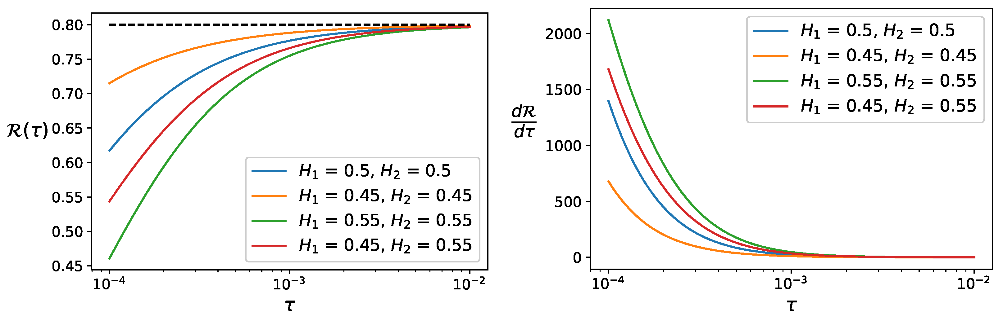
Figure 1 shows the correlation and derivative as a function of $\tau$ in the noisy fractional Brownian motion model under different combinations of Hurst exponents. The parameters are $\rho =0.8,{\rho }_{ϵ}=0,{\eta }_1={10}^{-5}$, and ${\eta }_2=2\times {10}^{-5}$. In other words, the two processes are correlated through the fractional Brownian motions, but their microstructure noises are independent. The correlation curves $\mathcal{R}\left(\tau \right)$ all increase in $\tau$ and approach the constant correlation coefficient $\rho =0.8$. This can be seen on the right panel as the slopes $d\mathcal{R}/d\tau$ start from a high value and decay to zero as $\tau$ goes from ${10}^{-4}$ to ${10}^{-2}$. The one associated with the highest Hurst exponent pair $(H_1=H_2=0.55)$ has the lowest correlation but also increases most rapidly as $\tau$ increases.

3.3.3. Correlation Curve Evaluation and Fitting

The correlation curve given by Equation (11) can be rather complicated, with six parameters, making it hard to evaluate against observation from real-world data. One practical approach is to consider the noisy Brownian motion model so that the correlation is given by Formula (13). Starting from this expression with only three parameters, $\rho ,{\eta }_1,{\eta }_2$, a simple rearrangement yields

$$\frac{1}{{\left(\mathcal{R}[Y_1,Y_2]\left(\tau \right)\right)}^2}=\frac{1}{{\rho }^2}\frac{(\tau +2{\eta }_1)(\tau +2{\eta }_2)}{{\tau }^2}=\frac{1}{{\rho }^2}\left(1+\frac{2{\eta }_1}{\tau }\right)\left(1+\frac{2{\eta }_2}{\tau }\right).$$

Next, if we define the frequency variable $\omega$: $=1/\tau$ and assume that ${\eta }_1,{\eta }_2\ll 1$, we have

$$\begin{array}{cc}\hfill \frac{1}{\mathcal{R}{[Y_1,Y_2]}^2}& =\frac{1}{{\rho }^2}(1+2({\eta }_1+{\eta }_2)\omega +4{\eta }_1{\eta }_2{\omega }^2)\hfill \end{array}$$

(14)

$$\begin{array}{cc}\hfill & \approx \frac{1}{{\rho }^2}+\frac{2({\eta }_1+{\eta }_2)}{{\rho }^2}\omega .\hfill \end{array}$$

(15)

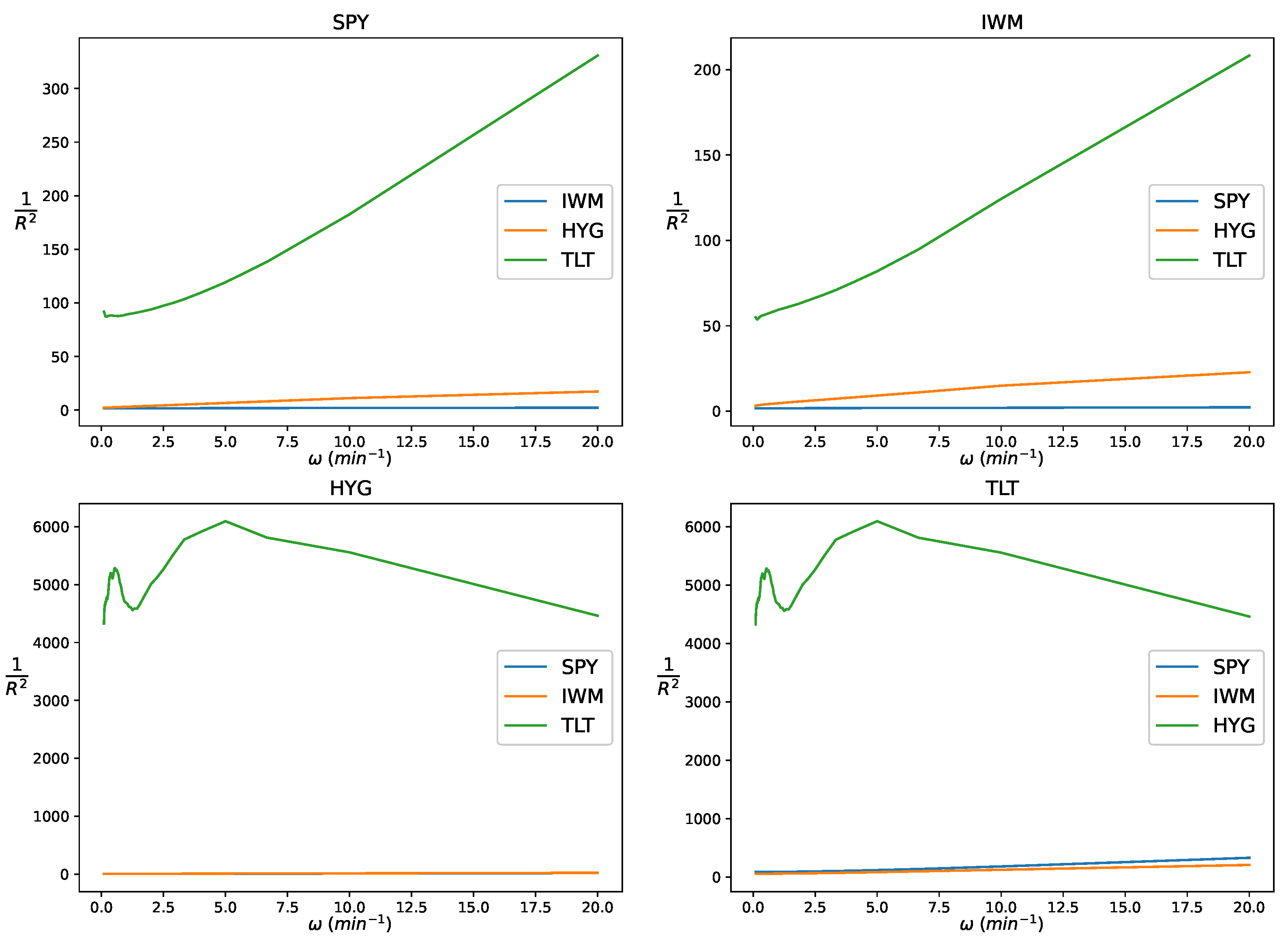
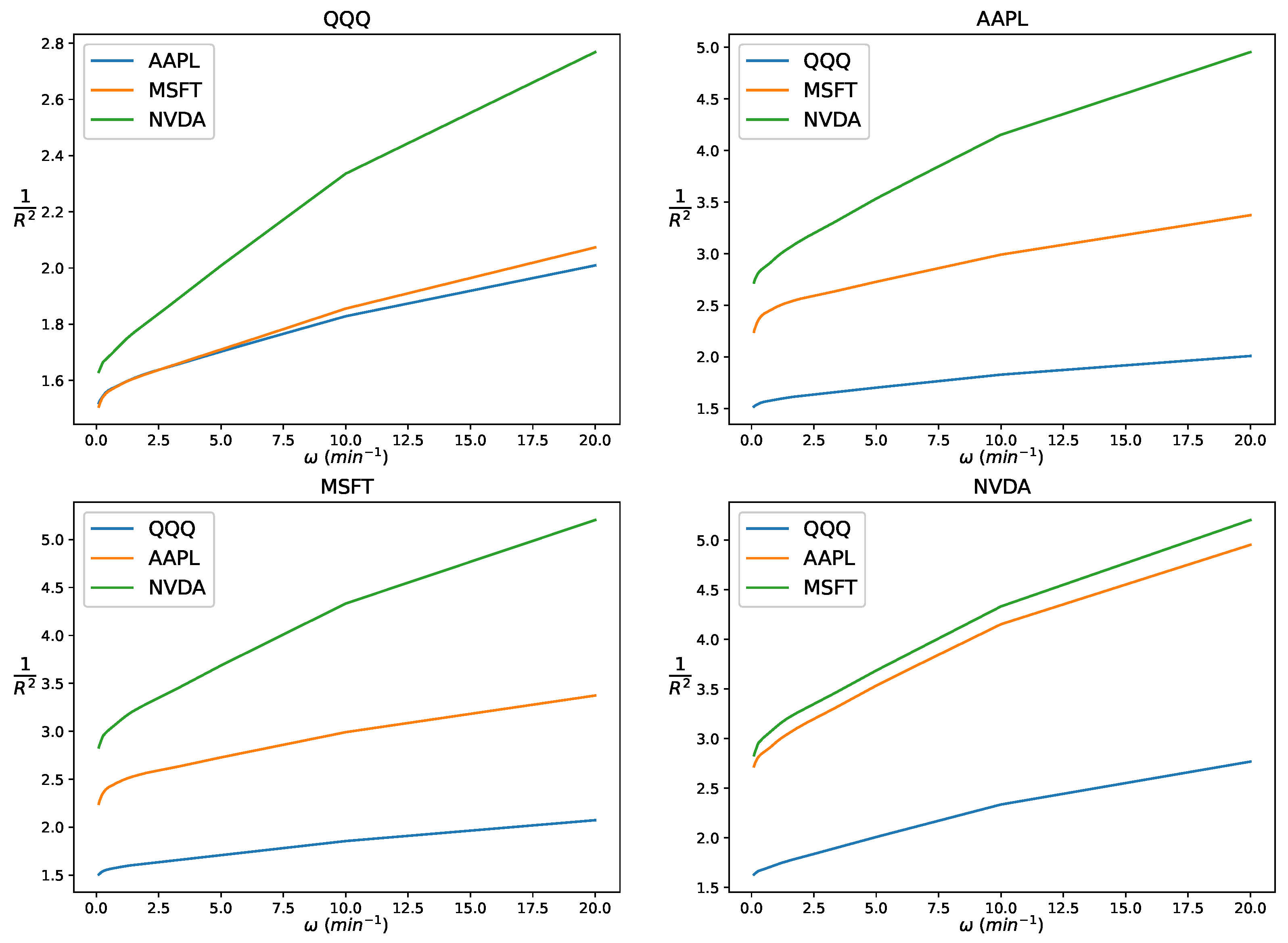
From (15), we observe that the inverse of the correlation squared can be approximated by a linear function in frequency $\omega :1/\tau$. The intercept is determined by ${\rho }^2$, and the slope is positive and depends on the summation of the two noise ratios ${\eta }_1+{\eta }_2$. We will return to this as we empirically verify this property with real-world data in the next section

Consider a collection of p noisy Brownian motions $Y_1,\cdots ,Y_p$, with corresponding noise ratios ${\eta }_1,\cdots ,{\eta }_p$. Suppose the correlation coefficient between the latent processes of $Y_i$ and $Y_j$ is ${\rho }_{ij}$; we can evaluate the parameters following the following procedure:

• Compute $R_{ij,m}$, $1\le i<j\le p$ using Equation (6), and ${\omega }_m=\frac{1}{m\delta t}$, for $m=1,\cdots ,M$.
• Fit linear regressions $\frac{1}{R_{ij,m}^2}={\alpha }_{ij}+{\beta }_{ij}{\omega }_m$ for $1\le i<j\le p$.
• Estimate the correlation $\widehat{{\rho }_{ij}}=\mathrm{sgn}\left(R_{ij,M}\right)\frac{1}{\sqrt{{\alpha }_{ij}}}$.
• Define the index mapping function $\xi (i,j)={\sum }_{l=1}^{i-1}(p-l)+(j-i)$, for $1\le i<j\le p$. The values of $\xi$ are $1,\cdots ,p(p-1)/2$.
• Construct the vector $\overrightarrow{b}\in {\mathbb{R}}^{p(p-1)/2}$, s.t. $b_{\xi (i,j)}=\frac{{\beta }_{ij}}{2{\alpha }_{ij}}$ for $1\le i<j\le p$.
• Construct the matrix $A\in {\mathbb{R}}^{p(p-1)/2\times p}$, s.t. $A_{k,i}=1$ if there exists $j>i$ s.t. $k=\xi (i,j)$ or $j<i$ s.t. $k=\xi (j,i)$; otherwise, $A_{k,i}=0$.
• Estimate the noise ratio vector $\widehat{\eta }=A^{†}\overrightarrow{b}.$

Here, $A^{†}$ represents the pseudo-inverse of A. For $\widehat{\eta }=A^{†}\overrightarrow{b}$ to be solvable, there must be $p\ge 3$ noisy Brownian motions in the collection. When $p=3$, A is invertible. When $p>3$, the matrix is over-determined.

4. Experiments on Intraday Data

In this section, we discuss the experimental results obtained using real-world high-frequency data of intraday prices sampled at 3 s intervals. Exchange-traded funds (ETFs) and stocks from different sectors are considered, with dates ranging from 27 January 2020 to 22 September 2023. On each trading day in the sample, the market is open for 6.5 h. The collection of equities covers a variety of types that can be categorized as follows:

• Broad market ETFs: SPY, IWM.
• Bond ETFs: HYG, TLT.
• Sector ETFs: XLK, XLF, XLP, XLY.
• Technology sector ETF and stocks: QQQ, AAPL, MSFT, NVDA.

4.1. Multiscale Correlation Curve

The assets are divided into three comparison groups and we analyze the multiscale correlation behavior among each group. The correlation Formula (6) allows us to compute the correlation curves for different asset pairs within one group.

4.1.1. Sector ETFs

In this group, we analyze the multiscale correlation among four sector ETFs, namely XLK, XLF, XLP, and XLY. Figure 2 shows the correlation curves for all of the pairs among the four ETFs, averaged over all dates in the dataset. From the plots, we can see that all of the correlation curves show a concave increasing shape, converging up to certain levels. This is clear evidence that the correlation between intraday price movements is scale-dependent. As we have shown in the previous sections, none of the Brownian motion, fractional Brownian motion, or stochastic volatility models yield such scale-dependent correlation. The shape of the curves are very similar to that of the noisy (fractional) Brownian motion model shown in Figure 1.

To further evaluate whether the real-world data match the correlation function of a noisy fractional Brownian motion model, we transformed the estimated curves to check if the data exhibit linearity according to (15). Then, using (15), we obtained the average correlation curves over all dates. Figure 3 shows the plots of $1/{\mathcal{R}}^2$ against $\omega$: $1/\tau$. From the figures, we can see approximately linear relations for all of the ticker pairs, indicating that the model could be a good fit. Nevertheless, we should also notice the bumpy shape when $\omega$ is very small, i.e., at large timescale. Even though only very small parts are shown on the plots, we should keep in mind that $\omega$: $=1/\tau$ is not evenly distributed on the x-axis. Therefore, there might be unexplained patterns at large timescales. Even though the noisy fractional Brownian motion model may not be a perfect fit for the whole dynamics of the data, it provides a theoretical framework to explain the correlation behavior existing in real-world high-frequency prices.

Following the fitting procedure for (15), we provide numerical estimation of the correlation and noise ratio parameters in

Table 1. Estimated parameters in multivariate noisy Brownian motion model using the correlation curves based on the intraday dataset. The first four columns show the estimated latent correlation matrix. The last column shows the noise ratio estimator ${\eta }_i$: $={\sigma }_{ϵ,i}^2/{\sigma }_i^2$.

	XLK	XLF	XLP	XLY	$\mathit{\eta }$ (${10}^{-2}$ min)
XLK	1	0.449211	0.354327	0.755362	0.580811
XLF	0.449211	1	0.450155	0.560384	3.719924
XLP	0.354327	0.450155	1	0.371876	1.674828
XLY	0.755362	0.560384	0.371876	1	1.761024

.

4.1.2. Stock vs. Bond

We now analyze the multiscale correlation between the equity ETFs, SPY and IWM, and the bond ETFs, HYG and TLT. Figure 4 shows the correlation curves for all of the pairs among the four ETFs, averaged over all dates in the dataset. While the sector ETFs are positively correlated, in the stock vs. bond case, we see a clear negative correlation between TLT and the two stock market ETFs. Even though the correlation sign is flipped, we can see that the absolute value for all the correlation curves show a concave increasing shape as before. The bond ETF pair, HLG and TLT, shows nearly zero correlation that is constant across the timescale studied, which is very different from all other pairs. The correlation curves among SPY, IWM, and HYG also show a positive concave increasing shape.

Similarly, we transform the estimated curves to check if the data fit the linear form in (15). Figure 5 shows the plots of $1/{\mathcal{R}}^2$ against $\omega$: $1/\tau$. From the figures, we can see approximately linear relations for pairs among stock ETFs and between stock and bond, indicating that the model could be a good fit. However, the trend is clearly different between the two bond ETFs, HYG and TLT, indicating that the dynamics between the bond ETFs cannot be explained by the noisy fractional Brownian motion model. The $1/{\mathcal{R}}^2$ value is also extremely high due to the low correlation between HYG and TLT.

The numerical estimations of the correlation and noise ratio parameters are summarized in

Table 2. Estimated parameters in multivariate noisy Brownian motion model using the correlation curves based on the intraday dataset. The first four columns show the estimated latent correlation matrix. The last column shows the noise ratio estimator ${\eta }_i$: $={\sigma }_{ϵ,i}^2/{\sigma }_i^2$.

	SPY	IWM	HYG	TLT	$\mathit{\eta }$ (${10}^{-2}$ min)
SPY	1	0.767284	0.616883	−0.120105	4.661190
IWM	0.767284	1	0.50646	−0.143798	3.237822
HYG	0.616883	0.50646	1	0.014145	6.159371
TLT	−0.120105	−0.143798	0.014145	1	1.014963

. We see a negative correlation between the stock ETFs and TLT as expected.

4.1.3. Technology Market and Stocks

Now, we turn to the three technology stocks, AAPL, MSFT, and NVDA, along with the technology market ETF, QQQ. Figure 6 shows the correlation curves for all of the pairs among the four ETFs, averaged over all dates in the dataset. Similar to the sector ETF case, from the plots, we can see that all of the correlation curves show a concave increasing shape, converging to certain levels. This is clear evidence that the correlation between intraday price movements is scale-dependent. The shapes of the curves are also very similar to that of the noisy (fractional) Brownian motion model shown in Figure 1.

As before, we transform the estimated curves to check if the data fit the linear form implied by (15). Figure 7 shows the plots of $1/{\mathcal{R}}^2$ against $\omega$: $1/\tau$. Similar to the sector ETF case, the plots show approximately linear relations for all of the ticker pairs, indicating that the model could be a good fit. Nevertheless, we should also notice the bumpy shape when $\omega$ is very small at large timescales. However, unlike the sector ETF case, the trend at large timescales for the technology stocks is going downwards. This indicates that the unexplained patterns at large timescales for the technology stocks trend towards a higher correlation. In contrast, the correlation for the sector ETFs drops at large timescales.

Following the fitting procedure for the correlation–frequency equation in (15), we provide a numerical estimation of the correlation and noise ratio parameters in

Table 3. Estimated parameters in multivariate noisy Brownian motion model using the correlation curves using the intraday dataset. The first four columns show the estimated latent correlation matrix. The last column shows the noise ratio estimator ${\eta }_i$: $={\sigma }_{ϵ,i}^2/{\sigma }_i^2$.

	QQQ	AAPL	MSFT	NVDA	$\mathit{\eta }$ (${10}^{-3}$ min)
QQQ	1	0.796396	0.798133	0.768358	2.960843
AAPL	0.796396	1	0.636989	0.585792	4.575938
MSFT	0.798133	0.636989	1	0.571759	5.063824
NVDA	0.768358	0.585792	0.571759	1	13.742560

.

4.2. Multiscale Correlation Time Series

For various ETFs and stocks, the estimated multiscale correlation does not stay constant over time. To see the evolution of multiscale correlation over time, we compute the 60-day rolling average of the correlation estimated at 3 s, 30 s, and 10 min scales. This is shown in Figure 8, Figure 9, Figure 10 and Figure 11.

Figure 8 shows the multiscale correlations among three ETFs: SPY, HYG, and TLT. While the SPY-HYG pair exhibits parallel correlation time series at the three timescales, the other two pairs show scale-crossing behavior when the correlation changes signs. We can see clearly that the correlations at all timescales approach zero at the same time, and the smallest timescales always have the smallest absolute correlation value. This is consistent with the noisy fractional Brownian motion model that we proposed. Figure 9 shows the multiscale correlation time series among three stocks from the same sector: AAPL, MSFT, and NVDA. We can see that all three pairs exhibit similar patterns, suggesting common behavior for the technology stocks.

In Figure 10 and Figure 11, we consider six ETF pairs using the four sector ETFs: XLK, XLF, XLP, and XLY. The correlation tends to be visibly lower at the larger timescale than at the small timescale. This pattern holds over multiple years. The correlations at the smaller timescales (i.e., 3 s and 30 s) become quite close over time. The scale dependency seems to be stronger at a higher frequency for the sector ETFs than technology stocks. Another interesting observation is that the correlation tends to dip in the middle of the year, most obviously in 2021 and 2023.

5. Conclusions

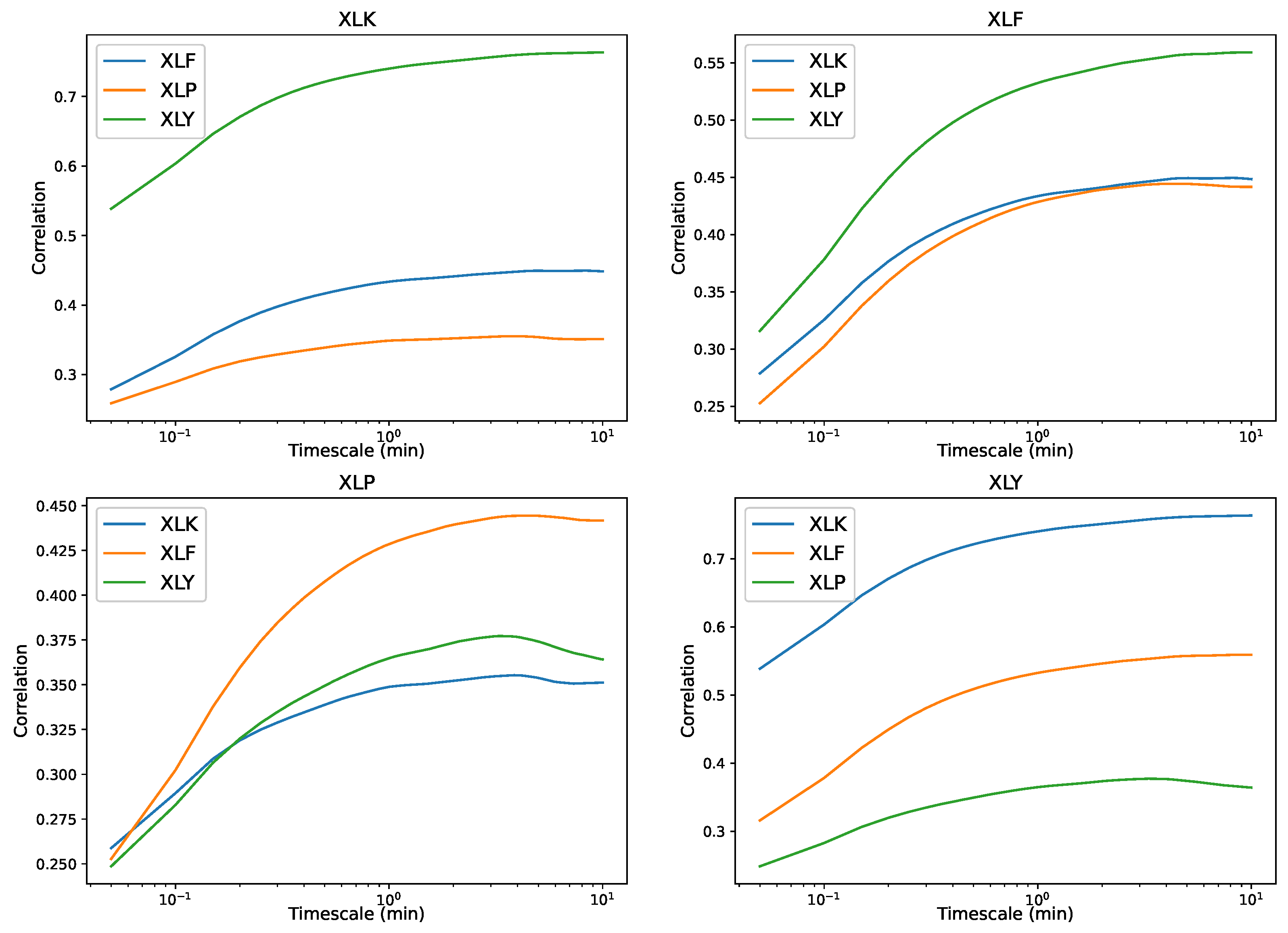
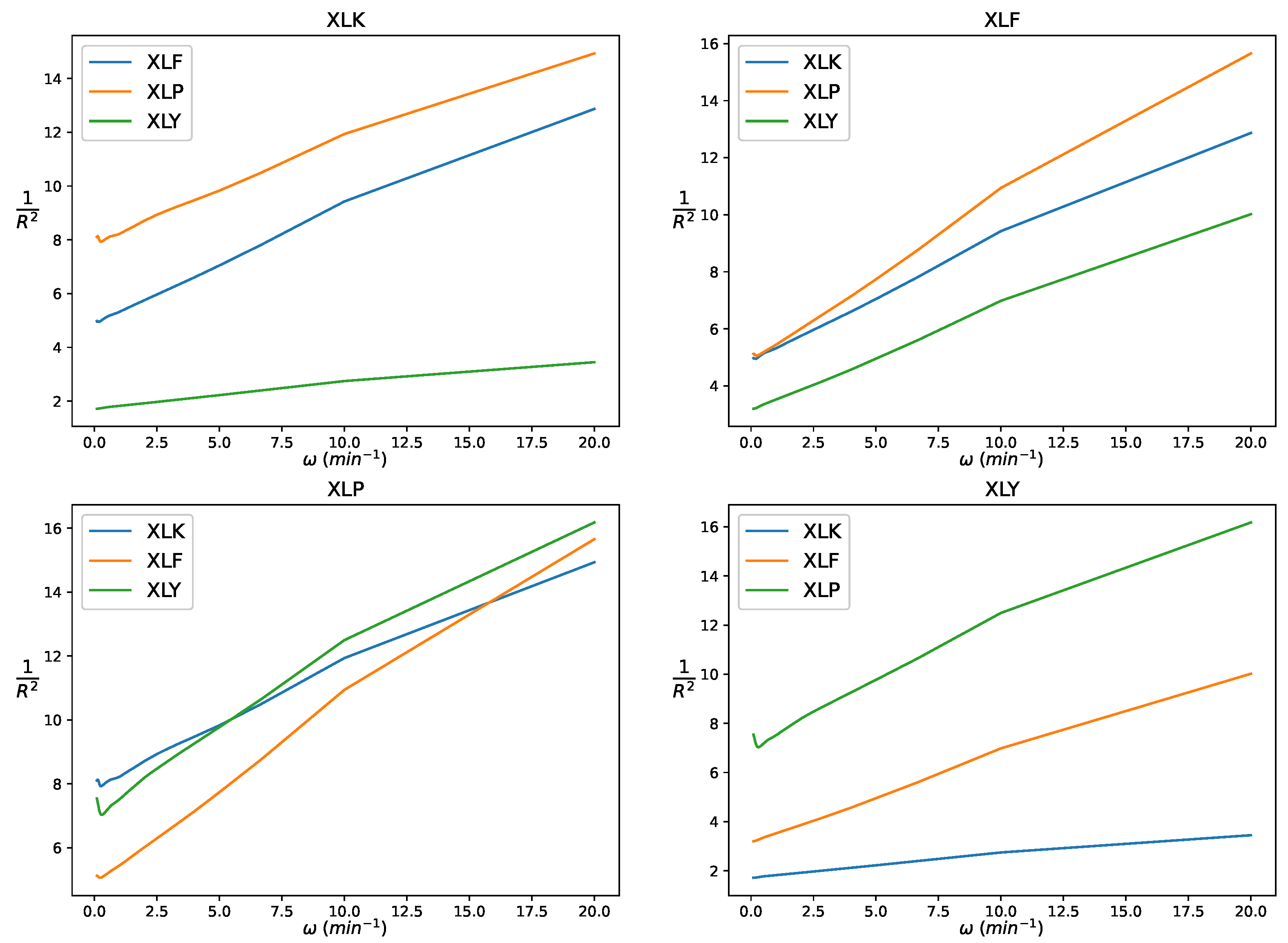
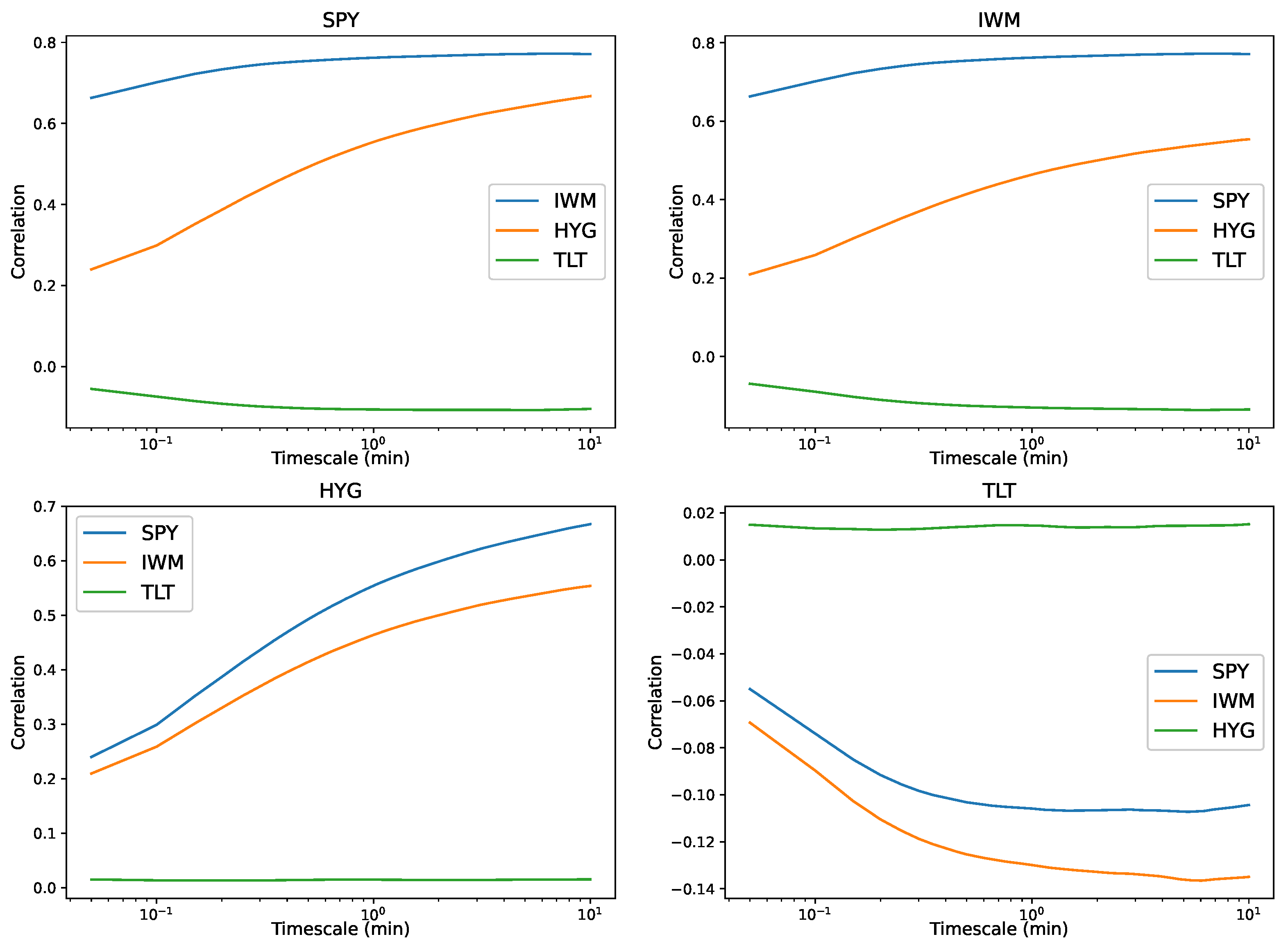
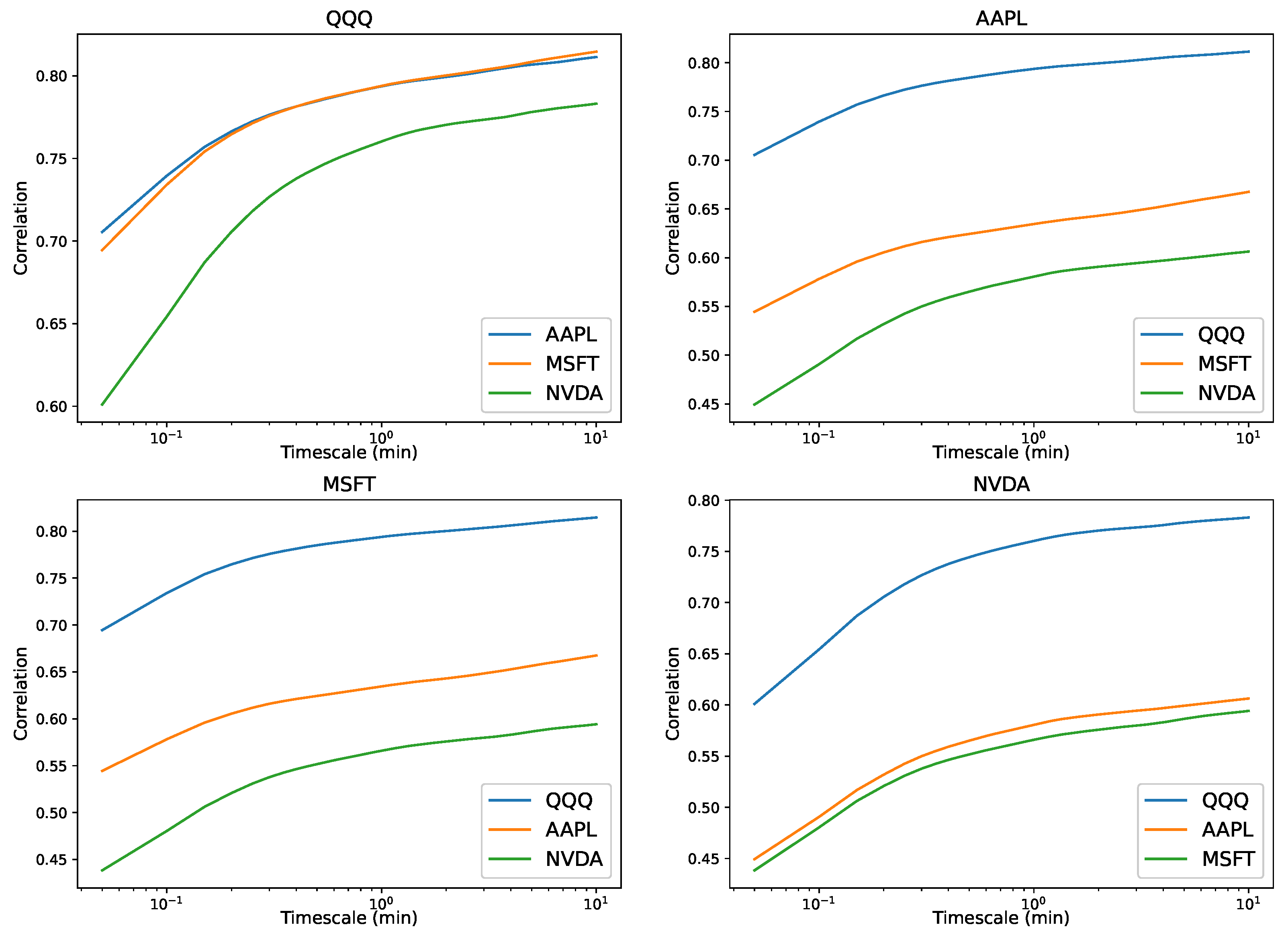
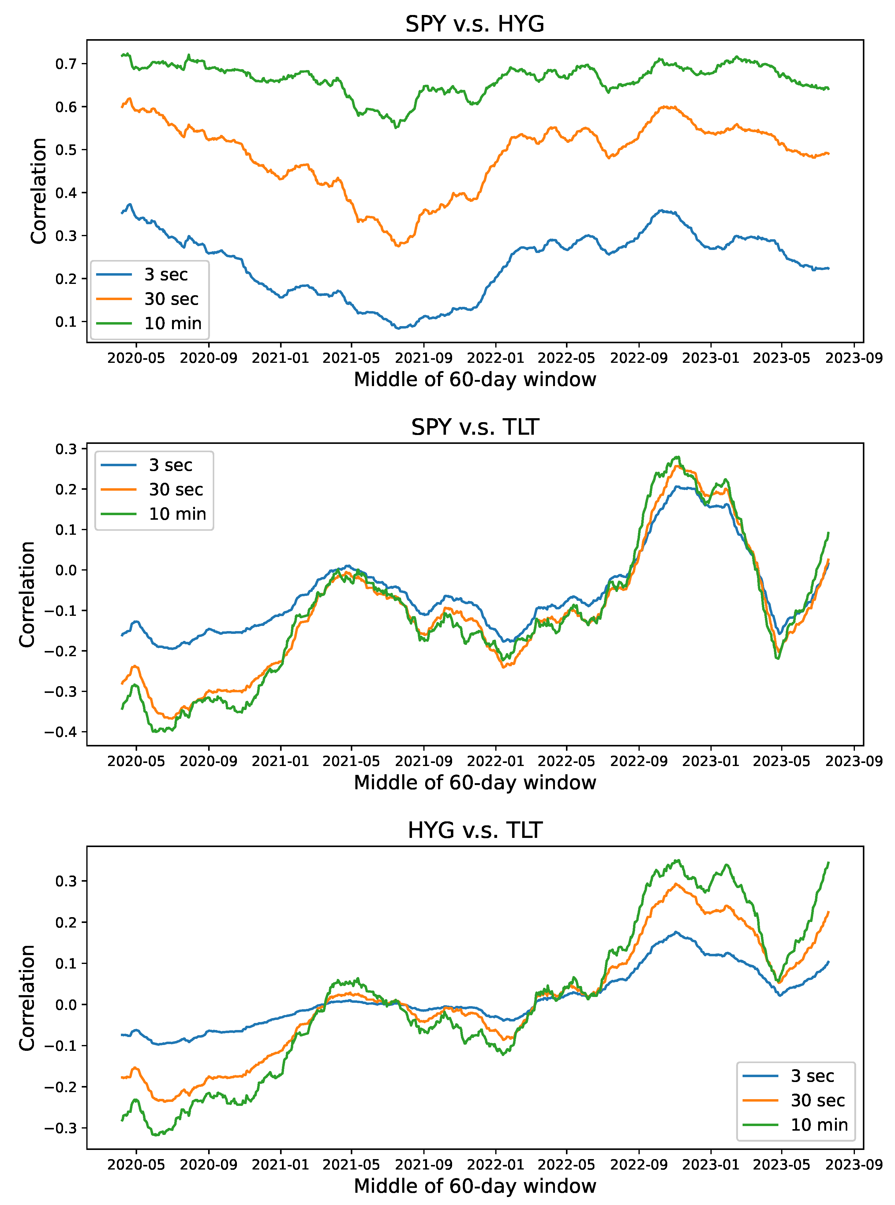
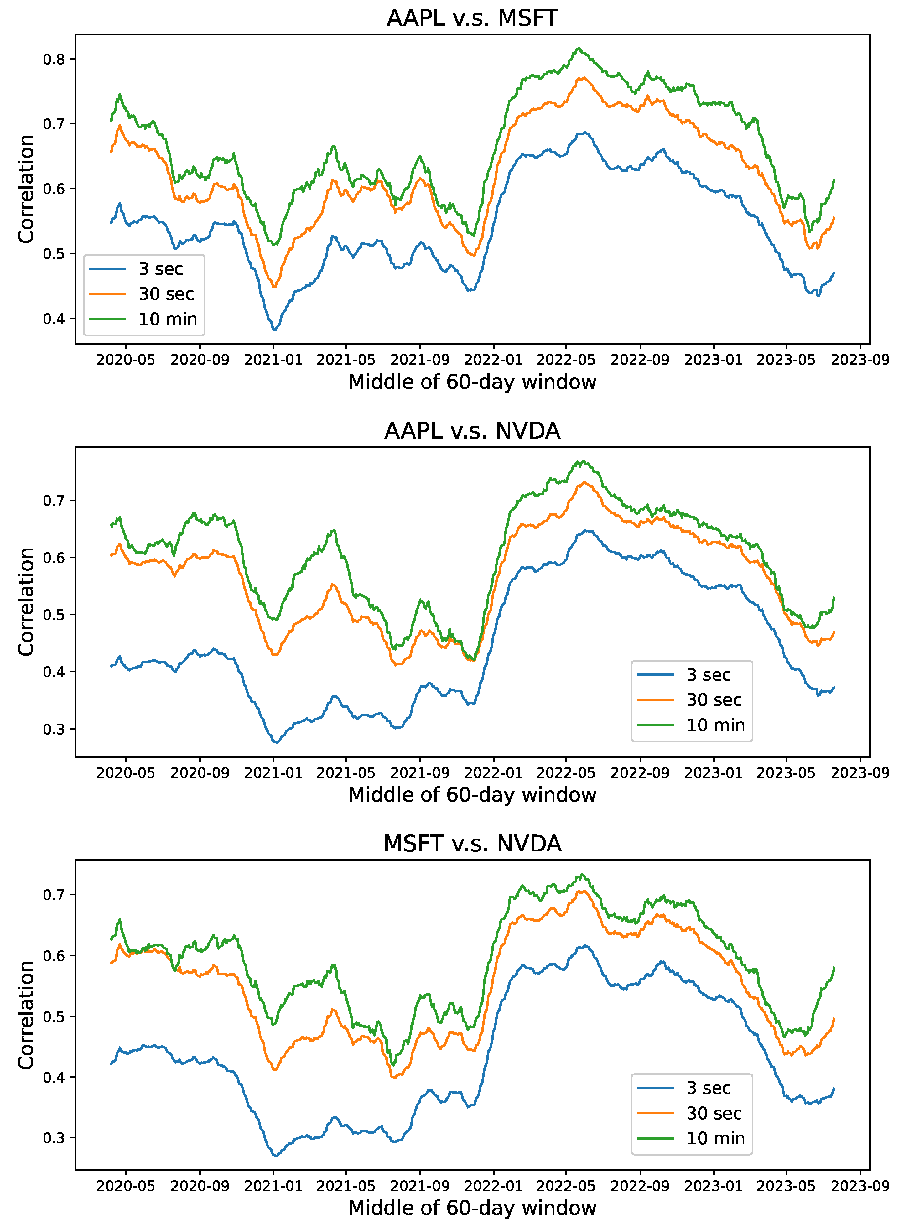
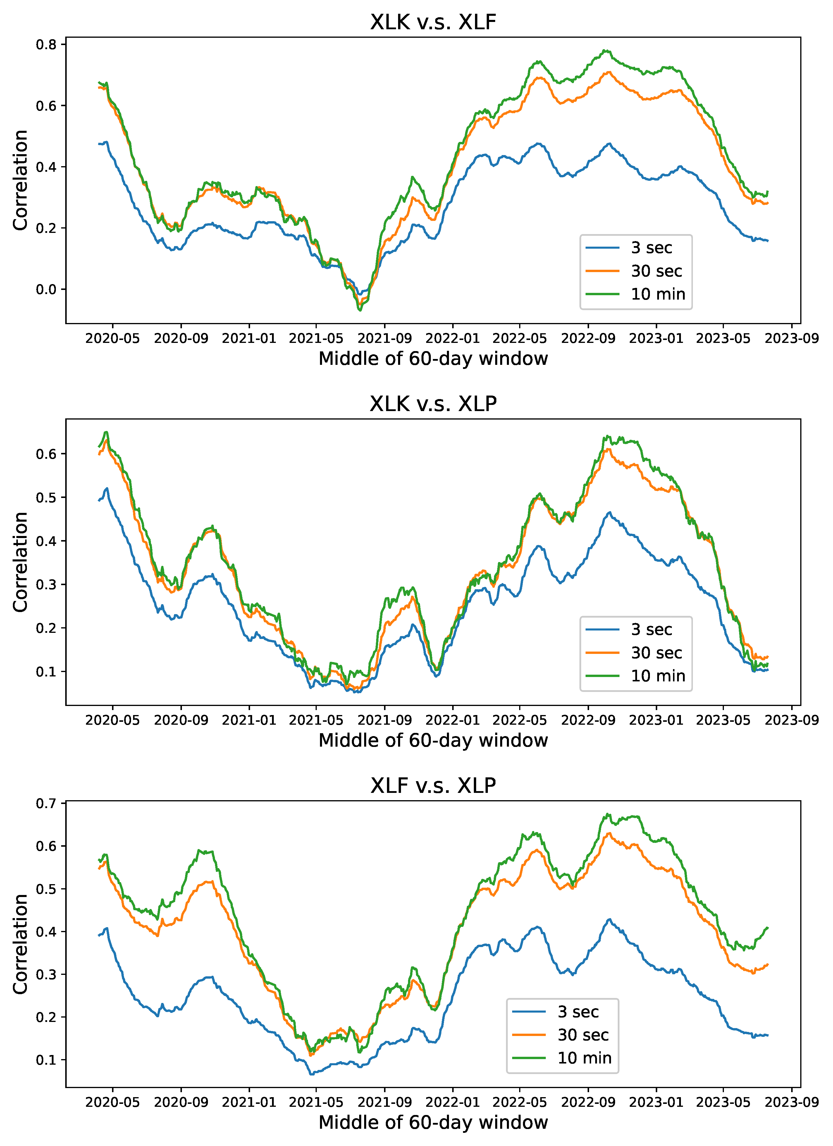
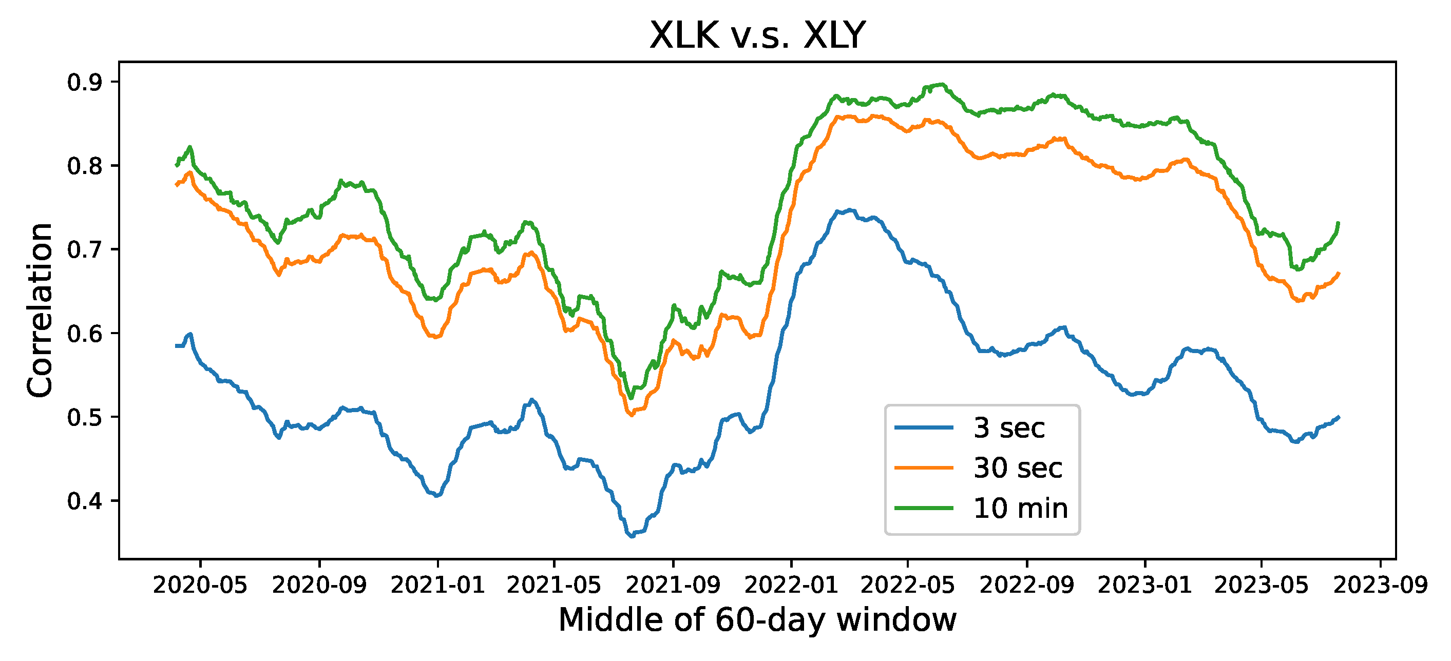
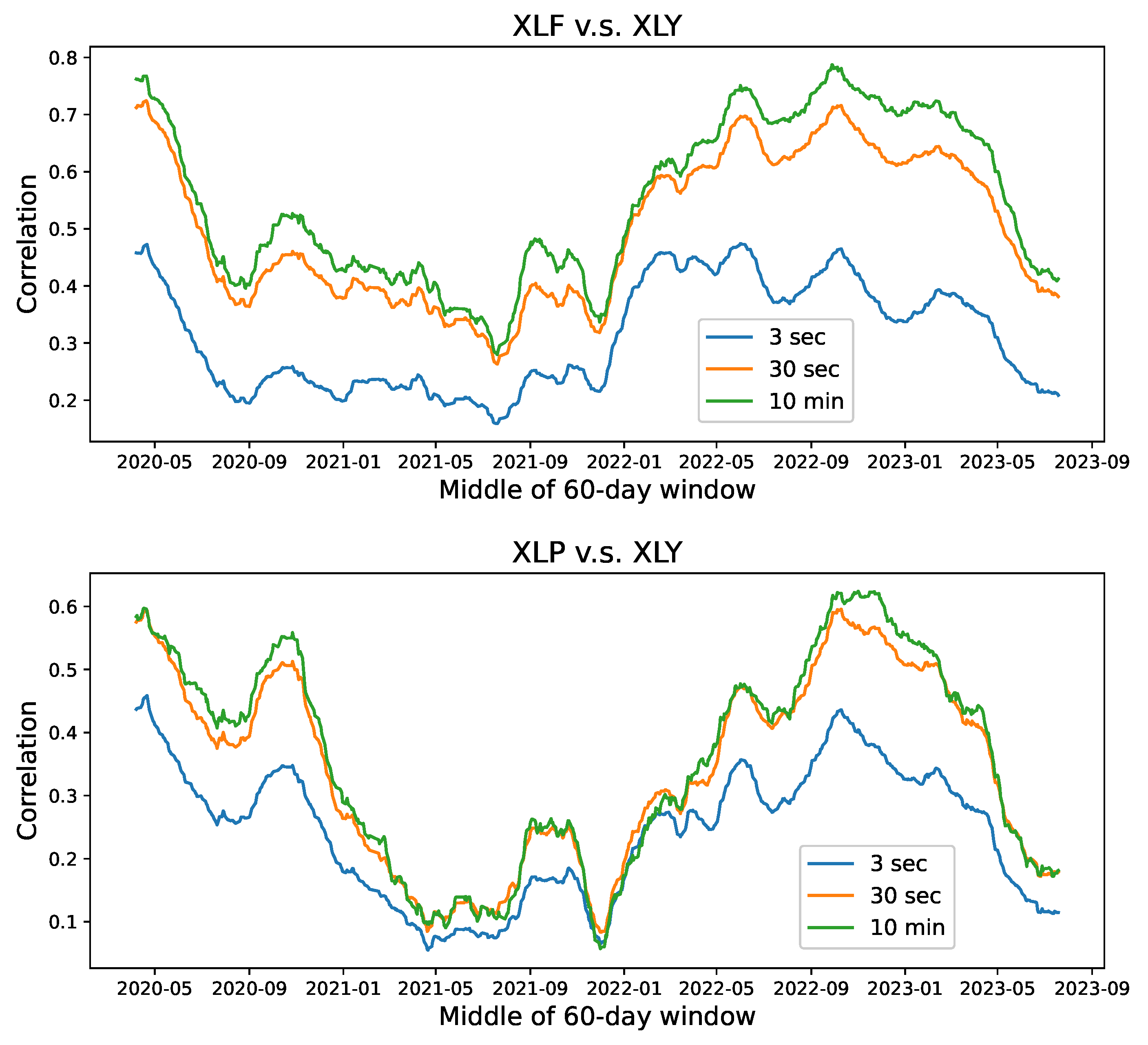
In this paper, we have presented a multiscale correlation analysis of noisy high-frequency financial data. The stochastic model studied herein is shown to possess a variety of statistical properties suitable for real-world intraday prices. To extract the correlation structure from prices, we devise a novel Hurst exponent estimator based on our model and estimate the exponent using a collection of major US stocks and ETFs. This helps better the understanding of the intraday correlations among asset prices and also the evolution of correlations over time.

The current study also suggests several future directions for further investigation. For instance, machine learning models can be designed to harness the Hurst exponents and other estimates from our model as useful inputs. There are a number of practical applications, including portfolio optimization and risk management at different timescales. Our current study illustrates that the Hurst exponent for different assets may vary significantly. This should motivate authors to conduct research on finding and understanding the factors that give rise to this phenomenon.

References

1. Osborne, M.F. Brownian motion in the stock market. Oper. Res. 1959, 7, 145–173. [Google Scholar] [CrossRef]
2. Mandelbrot, B. New methods in statistical economics. J. Political Econ. 1963, 71, 421–440. [Google Scholar] [CrossRef]
3. Mandelbrot, B.B.; Van Ness, J.W. Fractional brownian motions, fractional noises and applications. SIAM Rev. 1968, 10, 422–437. [Google Scholar] [CrossRef]
4. Rogers, L.C.G. Arbitrage with fractional brownian motion. Math. Financ. 1997, 7, 95–105. [Google Scholar] [CrossRef]
5. Guasoni, P.; Nika, Z.; Rásonyi, M. Trading fractional brownian motion. SIAM J. Financ. Math. 2019, 10, 769–789. [Google Scholar] [CrossRef]
6. Øksendal, B. Fractional Brownian Motion in Finance; Pure Mathematics Preprint Series; University of Oslo: Oslo, Norway, 2003; Available online: http://urn.nb.no/URN:NBN:no-8076 (accessed on 1 February 2024).
7. Capobianco, E. Multiscale stochastic dynamics in finance. Phys. A Stat. Mech. Its Appl. 2004, 344, 122–127. [Google Scholar] [CrossRef]
8. In, F.; Kim, S. An Introduction to Wavelet Theory in Finance: A Wavelet Multiscale Approach; World Scientific: Singapore, 2013. [Google Scholar]
9. Leung, T.; Zhao, T. Financial time series analysis and forecasting with hilbert–huang transform feature generation and machine learning. Appl. Stoch. Model. Bus. Ind. 2021, 37, 993–1016. [Google Scholar] [CrossRef]
10. Andersen, T.G.; Bollerslev, T.; Diebold, F.X. Some Like It Smooth, and Some Like It Rough: Untangling Continuous and Jump Components in Measuring, Modeling, and Forecasting Asset Return Volatility. 2003. Available online: https://ssrn.com/abstract=473204 (accessed on 1 February 2024).
11. Fan, J.; Wang, Y. Multi-scale jump and volatility analysis for high-frequency financial data. J. Am. Stat. Assoc. 2007, 102, 1349–1362. [Google Scholar] [CrossRef]
12. Mensi, W.; Rehman, M.U.; Shafiullah, M.; Al-Yahyaee, K.H.; Sensoy, A. High frequency multiscale relationships among major cryptocurrencies: Portfolio management implications. Financ. Innov. 2021, 7, 75. [Google Scholar] [CrossRef]
13. Barndorff-Nielsen, O.E.; Shephard, N. Econometric analysis of realized volatility and its use in estimating stochastic volatility models. J. R. Stat. Soc. Ser. B Stat. Methodol. 2002, 64, 253–280. [Google Scholar] [CrossRef]
14. Ait-Sahalia, Y.; Mykl, P.A.; Zhang, L. How often to sample a continuous-time process in the presence of market microstructure noise. Rev. Financ. Stud. 2005, 18, 351–416. [Google Scholar] [CrossRef]
15. Bandi, F.M.; Russell, J.R. Microstructure noise, realized volatility, and optimal sampling. Rev. Econ. Stud. 2008, 75, 339–369. [Google Scholar] [CrossRef]
16. Cont, R.; Das, P. Rough volatility: Fact or artefact? Sankhya B 2024. [Google Scholar] [CrossRef]
17. Hurst, H.E. Long-term storage capacity of reservoirs. Trans. Am. Soc. Civ. Eng. 1951, 116, 770–799. [Google Scholar] [CrossRef]
18. Aït-Sahalia, Y.; Fan, J.; Xiu, D. High-frequency covariance estimates with noisy and asynchronous financial data. J. Am. Stat. Assoc. 2010, 105, 1504–1517. [Google Scholar] [CrossRef]
19. Podolskij, M.; Vetter, M. Estimation of volatility functionals in the simultaneous presence of microstructure noise and jumps. Bernoulli 2009, 15, 634–658. [Google Scholar] [CrossRef]
20. Zhang, L.; Mykland, P.A.; ït-Sahalia, Y. A tale of two time scales: Determining integrated volatility with noisy high-frequency data. J. Am. Stat. Assoc. 2005, 100, 1394–1411. [Google Scholar] [CrossRef]
21. Bibinger, M.; Hautsch, N.; Malec, P.; Reiß, M. Estimating the quadratic covariation matrix from noisy observations: Local method of moments and efficiency. Ann. Stat. 2014, 42, 1312–1346. [Google Scholar] [CrossRef]
22. Leung, T.; Zhao, T. Multiscale volatility analysis for noisy high-frequency prices. Risks 2023, 11, 117. [Google Scholar] [CrossRef]
23. Biagini, F.; Hu, Y.; Øksendal, B.; Zhang, T. Stochastic Calculus for Fractional Brownian Motion and Applications; Springer Science & Business Media: Berlin/Heidelberg, Germany, 2008. [Google Scholar]
24. Amblard, P.-O.; Coeurjolly, J.-F. Identification of the multivariate fractional Brownian motion. IEEE Trans. Signal Process. 2011, 59, 5152–5168. [Google Scholar] [CrossRef]
25. Amblard, P.-O.; Coeurjolly, J.-F.; Lavancier, F.; Philippe, A. Basic properties of the multivariate fractional Brownian motion. arXiv 2010, arXiv:1007.0828. [Google Scholar]
26. Coeurjolly, J.-F.; Amblard, P.-O.; Achard, S. On multivariate fractional Brownian motion and multivariate fractional gaussian noise. In Proceedings of the 2010 18th European Signal Processing Conference, Aalborg, Denmark, 23–27 August 2010; pp. 1567–1571. [Google Scholar]
27. Coeurjolly, J.-F.; Amblard, P.-O.; Achard, S. Wavelet analysis of the multivariate fractional Brownian motion. ESAIM Probab. Stat. 2013, 17, 592–604. [Google Scholar] [CrossRef]
28. Mishura, I. Stochastic Calculus for Fractional Brownian Motion and Related Processes; Springer Science & Business Media: Berlin/Heidelberg, Germany, 2008; Volume 1929. [Google Scholar]
29. Lavancier, F.; Philippe, A.; Surgailis, D. Covariance function of vector self-similar processes. Stat. Probab. Lett. 2009, 79, 2415–2421. [Google Scholar] [CrossRef]
30. Black, F. Noise. J. Financ. 1986, 41, 528–543. [Google Scholar] [CrossRef]
31. Jacod, J.; Li, Y.; Zheng, X. Statistical properties of microstructure noise. Econometrica 2017, 85, 1133–1174. [Google Scholar] [CrossRef]
Figure 1. Multiscale correlation of the noisy Brownian motion model with different Hurst exponents. Left: correlation curves approaching the model correlation parameter ρ = 0.8 . Right: correlation derivative curves for different Hurst exponents.
Mathematics 12 00864 g001
Figure 2. Correlation curves for sector ETFs, estimated for 3 s intraday data. For algorithm, see Section 2.2. The curves shown in each plot are estimated and averaged over all dates in the sample.
Mathematics 12 00864 g002
Figure 3. Inverse of correlation squared vs. frequency on intraday data, 1 / R 2 vs. ω : = 1 / τ , for sector ETFs, estimated using 3 s intraday prices.
Mathematics 12 00864 g003
Figure 4. Correlation curves for stock vs. bond ETFs, estimated for 3 s intraday data using the algorithm in Section 2.2. Each curve shows the average estimated correlation over all available dates for each asset pair.
Mathematics 12 00864 g004
Figure 5. 1 / R 2 vs. ω : = 1 / τ plots for stock vs. bond, estimated for the 3 s intraday dataset. The transform using Equation (15) is applied to the average correlation curves over all dates.
Mathematics 12 00864 g005
Figure 6. Correlation curves among {QQQ, AAPL, MSFT, NVDA} estimated for 3 s intraday data. For the algorithm, we refer to Section 2.2. The curves shown in each plot are estimated and averaged over all dates in the sample.
Mathematics 12 00864 g006
Figure 7. 1 / R 2 vs. ω : = 1 / τ plots for technology market and stocks, estimated for the 3 s intraday dataset. Equation (15) is applied to the average correlation curves over all dates.
Mathematics 12 00864 g007
Figure 8. Multiscale correlation between stock and bond ETFs estimated for a 60-day rolling window. Correlations of intraday returns at different scales are estimated for each day and averaged over all dates in the rolling window.
Mathematics 12 00864 g008
Figure 9. Multiscale correlations among technology stocks estimated for a 60-day rolling window. Correlations of intraday returns at different scales are estimated for each day and averaged over all dates in the rolling window.
Mathematics 12 00864 g009
Figure 10. Multiscale correlations among 3 pairs of sector ETFs {XLK, XLF, XLP} estimated for a 60-day rolling window. Correlations of intraday returns at different scales are estimated for each day and averaged over all dates in the rolling window.
Mathematics 12 00864 g010
Figure 11. Multiscale correlations between XLY of 3 other sector ETFs {XLK, XLF, XLP} estimated for a 60-day rolling window. Correlations of intraday returns at different scales are estimated for each day and averaged over all dates in the rolling window.Multiscale correlation time series (Stock).
Mathematics 12 00864 g011aMathematics 12 00864 g011b