Analyzing Soliton Solutions of the Extended (3 + 1)-Dimensional Sakovich Equation

Abstract

This work focuses on the utilization of the generalized exponential rational function method (GERFM) to analyze wave propagation of the extended (3 + 1)-dimensional Sakovich equation. The demonstrated effectiveness and robustness of the employed method underscore its relevance to a wider spectrum of nonlinear partial differential equations (NPDEs) in physical phenomena. An examination of the physical characteristics of the generated solutions has been conducted through two- and three-dimensional graphical representations.

1. Introduction

Recently, the exploration of explicit and precise solutions for traveling waves in NPDEs has attracted significant attention from researchers. This interest stems from the potential applications of these solutions in various scientific and technological domains, especially in applied mathematics, hydrodynamics, quantum mechanics, solid-state physics, electron thermal energy, stochastic dynamical systems, nonlinear optics, and other related fields. Hence, the discovery of analytical solutions for these equations is crucial in comprehending their dynamics and elucidating the underlying mechanisms governing their existing states. Diverse researchers have successfully employed, developed, and refined a range of innovative approaches to obtain exact solutions for NPDEs, such as the modified and extended rational expansion method [1], the $G^{\prime }/$($b{G}^{\prime }+G+a$)-expansion technique [2], similarity transformations [3], the Hirota bilinear method [4], the homogenouous balance method [5], the tanh technique [6], Chupin Liu’s theorem [7], the first integral technique [8], auto-Backlund transformations [9], the sine-Gordon equation method [10], the modified $G^{\prime }/G$ -expansion method [11], the Riccati equation mapping method [12], the new Kudryashov technique [13], conservation laws [14,15], the Jacobian elliptic function expansion technique [16], Riccati–Bernoulli’s sub-ODE technique [17], the $sec{h}^p$ function method [18], Painlevé integrability [19], and so on.

The aim is to this paper is to explore analytical solutions for the newly extended (3 + 1)-dimensional Sakovich equation. The growing interest in researching nonlinear integrable equations is attributed to their ability to model crucial phenomena across various scientific disciplines, such as atmospheric sciences, oceanography, and related fields. In the context at hand, a notable exemplar of pertinent research is the following study. Sakovich presented a novel three-dimensional equation as follows [20]:

$${\varphi }_{xz}+{\varphi }_{yy}+2\varphi {\varphi }_{xy}+6{\varphi }^2{\varphi }_{xx}+2\left({\varphi }_{xx}^2\right)=0.$$

(1)

More recently, Wazwaz extended Equation (1) into a modified Sakovich equation in the following manner [21].

$${\varphi }_{xt}+{\varphi }_{xx}+{\varphi }_{xz}+{\varphi }_{yy}+{\varphi }_{xy}+{\varphi }_{yz}+2\varphi {\varphi }_{xy}+6{\varphi }^2{\varphi }_{xx}+2\left({\varphi }_{xx}^2\right)=0.$$

(2)

Numerous researchers have investigated Equation (2). For example, Singh and Ray [22] derived an auto-Bäcklund transformation and conducted Painlevé analysis on Equation (2) to generate soliton solutions. The same equation has been investigated using the Painlevé test, and multiple soliton solutions have been derived [23,24]. Recently, Wazwaz transformed Equation (2) into the newly formulated (3 + 1)-dimensional Sakovich equation as follows [25]:

$${\varphi }_{xt}+{\varphi }_{xx}+{\varphi }_{yy}+{\varphi }_{zz}+{\varphi }_{xy}+{\varphi }_{xz}+{\varphi }_{yz}+2\varphi {\varphi }_{xy}+6{\varphi }^2{\varphi }_{xx}+2{\left({\varphi }_{xx}\right)}^2+\varphi {\varphi }_{xx}=0.$$

(3)

Here, the function $\varphi$ represents the relationship with the 3D spatial variables and the temporal variable. This newly formulated equation demonstrates a broader range of practical applications from a physical standpoint when compared to the two aforementioned equations. Due to its ability to capture increased dispersion and nonlinear effects, it proves suitable for various utilizations. A multi-soliton analysis of Equation (3) was conducted, and its integrability was assessed using the Painlevé test [25]. Ali et al. [26] utilized the $G^{\prime }/$($b{G}^{\prime }+G+a$)-expansion and exp(-$\psi$($\xi$)) procedure to identify analytical solutions for the equation. Cortez et al. identified Lie symmetries of Equation (3) [27].

The primary goal of this work is to analyze the propagation of waves in the newly formulated (3 + 1)-dimensional Sakovich equation. The structure of this paper is delineated in the following manner: Section 2 provides an introduction to the GERFM. In Section 3, solitary wave solutions of the investigated equation are presented. Section 4 provides graphical depictions of diverse analytical solutions. Finally, the Conclusions section encapsulates the main discoveries of this paper.

2. The Methodology of GERFM

A description of the GERFM approach will be given in this section.

The general form of the NPDE is given as follows [28]:

$$F(\varphi ,{\varphi }_x,{\varphi }_y,{\varphi }_z,{\varphi }_t,{\varphi }_{xx},{\varphi }_{xt},...)=0,$$

(4)

where F is a polynomial of $\varphi \left(x,y,z,t\right)$ and its partial derivatives. By utilizing a wave transformation in the subsequent manner

$$\varphi (x,y,z,t)=\varphi \left(\xi \right),\xi =\alpha x+\beta y+\gamma z-\omega t,$$

(5)

we derive a nonlinear ordinary differential equation (ODE):

$$Q\left(\varphi ,{\varphi }^{\prime },{\varphi }^{″},{\varphi }^{‴},\dots \right)=0.$$

(6)

We consider the analytical solution of Equation (4):

$$\varphi \left(\xi \right)={\rho }_0+\sum _{n=1}^N{\rho }_n{\psi }^n\left(\xi \right)+\sum _{n=1}^N{b}_n{\psi }^{-n}\left(\xi \right),$$

(7)

$$\psi \left(\xi \right)=\frac{{\tau }_1{e}^{{\varsigma }_1\xi }+{\tau }_2{e}^{{\varsigma }_2\xi }}{{\tau }_3{e}^{{\varsigma }_3\xi }+{\tau }_4{e}^{{\varsigma }_4\xi }},$$

(8)

where ${\tau }_k,{\varsigma }_k(1\le k\le 4)$ exhibit the real (or complex) numbers that are later obtained, and ${\rho }_0,{\rho }_n,b_n,$$\left(1\le n\le N\right)$. The solution of Equation (7) will hold for Equation (6). The presence of N is ascertainable within the framework of the balancing principle. Substituting (7) into Equation (6) and collecting similar terms, we derive the polynomial equation $A(B_1,B_2,B_3,B_4)=0$ in terms of $B_i=e^{{\varsigma }_i\xi }$ for $i=1,...,4$. By setting the coefficients of A to zero, a system of algebraic expressions in ${\tau }_k,{\varsigma }_k(1\le k\le 4)$ and $\alpha ,\beta ,\gamma ,\omega ,{\rho }_0,{\rho }_n,b_n(1\le n\le 4)$ is reached. The solutions to Equation (4) are then determined by evaluating the derived expressions.

Remark 1. 

By setting ${\tau }_1={\tau }_3={\tau }_4=1,$ ${\tau }_2={\varsigma }_1={\varsigma }_2={\varsigma }_3=0$, ${\varsigma }_4=1$, and ${\beta }_n(n=1,...,N)$ in Equation (7) and Equation (8), the ERF approach is thus obtained [29].

$$\phi \left(\xi \right)=\frac{1}{1+e^{\epsilon }},$$

(9)

$$\varphi \left(\xi \right)={\rho }_0+\sum _{n=1}^m\frac{{\rho }_n}{{(1+e^{\xi })}^n}.$$

(10)

3. Applications

In this section, the procedures will be applied to the model provided in this section. By substituting the expression given in Equation (5) into Equation (3), the resulting equation is obtained:

$$\begin{array}{c}{\varphi }^{″}(-\omega \alpha +{\alpha }^2+{\beta }^2+{\gamma }^2+\alpha \beta +\alpha \gamma +\beta \gamma )\hfill \\ +\varphi {\varphi }^{″}({\alpha }^2+2\alpha \beta )+6{\alpha }^2{\varphi }^2{\varphi }^{″}+2{\alpha }^2{\left({\varphi }^{″}\right)}^2=0.\hfill \end{array}$$

(11)

Here, the balancing number is $N=2.$ Therefore, the solution will take the following form:

$$\varphi \left(\xi \right)={\rho }_0+{\rho }_1\psi \left(\xi \right)+{\rho }_2{\psi }^2\left(\xi \right)+\frac{b_1}{\psi \left(\xi \right)}+\frac{b_2}{{\psi }^2\left(\xi \right)},$$

(12)

where $\psi \left(\xi \right)$ is exhibited by Equation (8). By substituting Equation (12) into Equation (11) and gathering all the same terms, these equations are transformed into polynomials of $A(B_1,B_2,B_3,B_4)=0,\alpha ,\beta ,\gamma$ and $\omega .$

Family 1: Setting

$$\begin{array}{cccc}{\tau }_1=i,\hfill & {\tau }_2=i,\hfill & {\tau }_3=1,\hfill & {\tau }_4=-1,\hfill \\ {\varsigma }_1=i,\hfill & {\varsigma }_2=-i,\hfill & {\varsigma }_3=i,\hfill & {\varsigma }_4=-i,\hfill \end{array}$$

(13)

in Equation (8), one acquires

$$\psi \left(\xi \right)=\frac{cos\left(\xi \right)}{sin\left(\xi \right)},$$

(14)

From the substitution of Equation (14) into Equations (7) and (12), we find an equation system. Subsequently, we find the solutions of this system utilizing Maple and obtain the ensuing outcomes:

Case 1.1:

$$\begin{array}{c}{\rho }_0=-\frac{17\alpha +2\beta }{12\alpha },{\rho }_1=0,{\rho }_2=-2,b_1=0,\hfill \\ b_2=0,\omega =\frac{20{\beta }^2+20\alpha \beta +24\beta \gamma +87{\alpha }^2+24\alpha \gamma +24{\gamma }^2}{24\alpha }.\hfill \end{array}$$

(15)

Substituting the values from Equations (14) and (15) into Equation (12) yields the explicit solution for the investigated equation as follows:

$${\varphi }_{1,1}\left(\xi \right)=-\frac{17\alpha +2\beta }{12\alpha }-\frac{2{cos}^2\left(\xi \right)}{{sin}^2\left(\xi \right)},$$

(16)

where $\xi =\alpha x+\beta y+\gamma z-\frac{20{\beta }^2+20\alpha \beta +24\beta \gamma +87{\alpha }^2+24\alpha \gamma +24{\gamma }^2}{24\alpha }t.$

Case 1.2:

$$\begin{array}{c}{\rho }_0=-\frac{17\alpha +2\beta }{12\alpha },{\rho }_1=0,{\rho }_2=0,b_1=0,\hfill \\ b_2=-2,\omega =\frac{20{\beta }^2+20\alpha \beta +24\beta \gamma +87{\alpha }^2+24\alpha \gamma +24{\gamma }^2}{24\alpha }.\hfill \end{array}$$

(17)

Substituting the values from Equations (14) and (17) into Equation (12) yields the explicit solution for the investigated equation as follows:

$${\varphi }_{1,2}\left(\xi \right)=-\frac{17\alpha +2\beta }{12\alpha }-\frac{2{sin}^2\left(\xi \right)}{{cos}^2\left(\xi \right)},$$

(18)

where $\xi =\alpha x+\beta y+\gamma z-\frac{20{\beta }^2+20\alpha \beta +24\beta \gamma +87{\alpha }^2+24\alpha \gamma +24{\gamma }^2}{24\alpha }t.$

Case 1.3:

$$\begin{array}{c}{\rho }_0=-\frac{17\alpha +2\beta }{12\alpha },{\rho }_1=0,{\rho }_2=-2,b_1=0,\hfill \\ b_2=-2,\omega =\frac{20{\beta }^2+20\alpha \beta +24\beta \gamma +1047{\alpha }^2+24\alpha \gamma +24{\gamma }^2}{24\alpha }.\hfill \end{array}$$

(19)

Inserting Equations (14) and (19) into Equation (12), we find the exact solution of Equation (3) as follows:

$${\varphi }_{1,3}\left(\xi \right)=-\frac{17\alpha +2\beta }{12\alpha }-\frac{2{cos}^2\left(\xi \right)}{{sin}^2\left(\xi \right)}-\frac{2{sin}^2\left(\xi \right)}{{cos}^2\left(\xi \right)},$$

(20)

Family 2: Fixing

$$\begin{array}{cccc}{\tau }_1=1,\hfill & {\tau }_2=1,\hfill & {\tau }_3=1,\hfill & {\tau }_4=-1,\hfill \\ {\varsigma }_1=1,\hfill & {\varsigma }_2=-1,\hfill & {\varsigma }_3=1,\hfill & {\varsigma }_4=-1,\hfill \end{array}$$

(21)

in Equation (8), one acquires

$$\psi \left(\xi \right)=\frac{cosh\left(\xi \right)}{sinh\left(\xi \right)}.$$

(22)

From the substitution of Equation (22) into Equations (7) and (12), we find an equation system. Subsequently, we find the solutions of this system utilizing Maple and obtain the ensuing outcomes:

Case 2.1:

$$\begin{array}{c}{\rho }_0=\frac{15\alpha -2\beta }{12\alpha },{\rho }_1=0,{\rho }_2=-2,b_1=0,\hfill \\ b_2=-2,\omega =\frac{24{\gamma }^2+1047{\alpha }^2+20\alpha \beta +20{\beta }^2+24\alpha \gamma +24\beta \gamma }{24\alpha }.\hfill \end{array}$$

(23)

From the substitution of Equations (22) and (23) into Equation (12), we find the anaytical solution of the scrutinized equation as follows:

$${\varphi }_{2,1}\left(\xi \right)=\frac{15\alpha -2\beta }{12\alpha }-\frac{2{cosh}^2\left(\xi \right)}{{sinh}^2\left(\xi \right)}-\frac{2{sinh}^2\left(\xi \right)}{{cosh}^2\left(\xi \right)},$$

(24)

where $\xi =\alpha x+\beta y+\gamma z-\frac{24{\gamma }^2+1047{\alpha }^2+20\alpha \beta +20{\beta }^2+24\alpha \gamma +24\beta \gamma }{24\alpha }t.$

Case 2.2:

$$\begin{array}{c}{\rho }_0=\frac{15\alpha -2\beta }{12\alpha },{\rho }_1=0,{\rho }_2=0,b_1=0,\hfill \\ b_2=-2,\omega =\frac{20{\beta }^2+20\alpha \beta +24\beta \gamma +87{\alpha }^2+24\alpha \gamma +24{\gamma }^2}{24\alpha }.\hfill \end{array}$$

(25)

Substituting Equations (22) and (25) into Equation (12), we find the analytical solution of Equation (3) as follows:

$${\varphi }_{2,2}\left(\xi \right)=\frac{15\alpha -2\beta }{12\alpha }-\frac{2{sinh}^2\left(\xi \right)}{{cosh}^2\left(\xi \right)},$$

(26)

where $\xi =\alpha x+\beta y+\gamma z-\frac{20{\beta }^2+20\alpha \beta +24\beta \gamma +87{\alpha }^2+24\alpha \gamma +24{\gamma }^2}{24\alpha }t.$

Case 2.3:

$$\begin{array}{c}{\rho }_0=\frac{15\alpha -2\beta }{12\alpha },{\rho }_1=0,{\rho }_2=-2,b_1=0,\hfill \\ b_2=0,\omega =\frac{20{\beta }^2+20\alpha \beta +24\beta \gamma +87{\alpha }^2+24\alpha \gamma +24{\gamma }^2}{24\alpha }.\hfill \end{array}$$

(27)

From the substitution of Equations (22) and (27) into Equation (12), one finds the analytical solution of the scrutinized equation as follows:

$${\varphi }_{2,3}\left(\xi \right)=\frac{15\alpha -2\beta }{12\alpha }-\frac{2{cosh}^2\left(\xi \right)}{{sinh}^2\left(\xi \right)},$$

(28)

where $\xi =\alpha x+\beta y+\gamma z-\frac{20{\beta }^2+20\alpha \beta +24\beta \gamma +87{\alpha }^2+24\alpha \gamma +24{\gamma }^2}{24\alpha }t.$

Family 3: Setting

$$\begin{array}{cccc}{\tau }_1=2,\hfill & {\tau }_2=3,\hfill & {\tau }_3=1,\hfill & {\tau }_4=1,\hfill \\ {\varsigma }_1=1,\hfill & {\varsigma }_2=0,\hfill & {\varsigma }_3=1,\hfill & {\varsigma }_4=0,\hfill \end{array}$$

(29)

in Equation (8), one acquires

$$\psi \left(\xi \right)=\frac{3+2e^{\xi }}{1+e^{\xi }}.$$

(30)

From the substitution of Equation (30) into Equations (7) and (12), we find an equation system. Subsequently, we find the solutions of this system utilizing Maple and obtain the ensuing results:

Case 3.1:

$$\begin{array}{c}{\rho }_0=-\frac{147\alpha +2\beta }{12\alpha },{\rho }_1=10,{\rho }_2=-2,b_1=0,\\ b_2=0,\omega =\frac{27{\alpha }^2+20{\beta }^2+24{\gamma }^2+24\alpha \gamma +24\beta \gamma +20\alpha \beta }{24\alpha }.\end{array}$$

(31)

From the substitution of Equations (30) and (31) into Equation (12), one finds the analytical solution of the scrutinized equation as follows:

$${\varphi }_{3,1}\left(\xi \right)=\frac{9\alpha -2\beta -3\alpha cosh\left(\xi \right)-2\beta cosh\left(\xi \right)}{12\alpha \left(1+cosh\left(\xi \right)\right)},$$

(32)

where $\xi =\alpha x+\beta y+\gamma z-\frac{27{\alpha }^2+20{\beta }^2+24{\gamma }^2+24\alpha \gamma +24\beta \gamma +20\alpha \beta }{24\alpha }t.$

Case 3.2:

$$\begin{array}{c}{\rho }_0=-\frac{147\alpha +2\beta }{12\alpha },{\rho }_1=0,{\rho }_2=0,b_1=60,\hfill \\ b_2=-72,\omega =\frac{27{\alpha }^2+20{\beta }^2+24{\gamma }^2+24\alpha \gamma +24\beta \gamma +20\alpha \beta }{24\alpha }.\hfill \end{array}$$

(33)

From the substitution of Equations (30) and (33) into Equation (12), one finds the analytical solution of the scrutinized equation as follows:

$${\varphi }_{3,2}\left(\xi \right)=\frac{sinh\left(\xi \right)\left(10\beta +15\alpha \right)-cosh\left(\xi \right)\left(39\alpha +26\beta \right)+108\alpha -24\beta }{12\alpha \left(12+13cosh\left(\xi \right)-5sinh\left(\xi \right)\right)},$$

(34)

where $\xi =\alpha x+\beta y+\gamma z-\frac{27{\alpha }^2+20{\beta }^2+24{\gamma }^2+24\alpha \gamma +24\beta \gamma +20\alpha \beta }{24\alpha }t.$

Family 4: Setting

$$\begin{array}{cccc}{\tau }_1=i,\hfill & {\tau }_2=-i,\hfill & {\tau }_3=1,\hfill & {\tau }_4=1,\hfill \\ {\varsigma }_1=i,\hfill & {\varsigma }_2=-i,\hfill & {\varsigma }_3=i,\hfill & {\varsigma }_4=-i,\hfill \end{array}$$

(35)

in Equation (8), one acquires

$$\psi \left(\xi \right)=-\frac{sin\left(\xi \right)}{cos\left(\xi \right)},$$

(36)

From the substitution of Equation (36) into Equations (7) and (12), one finds an equation system. Subsequently, we find the solutions of this system utilizing Maple and obtain the ensuing outcomes:

Case 4.1: Substituting Equations (17) and (36) into Equation (12), one finds the solitary wave solution of Equation (3), the same as Equation (16).

Case 4.2: Substituting Equations (15) and (36) into Equation (12), one finds the solitary wave solution of Equation (3), the same as Equation (18).

Case 4.3: Substituting Equations (19) and (36) into Equation (12), one finds the solitary wave solution of Equation (3), the same as Equation (20).

Family 5: Setting

$$\begin{array}{cccc}{\tau }_1=3,\hfill & {\tau }_2=2,\hfill & {\tau }_3=1,\hfill & {\tau }_4=1,\hfill \\ {\varsigma }_1=1,\hfill & {\varsigma }_2=0,\hfill & {\varsigma }_3=1,\hfill & {\varsigma }_4=0,\hfill \end{array}$$

(37)

in Equation (8), one acquires

$$\psi \left(\xi \right)=-\frac{1}{e^{\xi }+1}.$$

(38)

From the substitution of Equation (38) into Equations (7) and (12), one finds an equation system. Subsequently, we find the solutions of this system utilizing Maple and obtain the ensuing results:

Case 5.1:

$$\begin{array}{c}{\rho }_0=-\frac{3\alpha +2\beta }{12\alpha },{\rho }_1=-2,{\rho }_2=-2,b_1=0,\hfill \\ b_2=0,\omega =\frac{24\beta \gamma +20\alpha \beta +27{\alpha }^2+24\alpha \gamma +20{\beta }^2+24{\gamma }^2}{24\alpha }\hfill \end{array}$$

(39)

Substituting Equations (38) and (39) into Equation (12), one finds the analytical solution of the scrutinized equation:

$${\varphi }_{5,1}\left(\xi \right)=\frac{9\alpha -2\beta -cosh\left(\xi \right)(3\alpha +2\beta )}{12\alpha \left(1+cosh\left(\xi \right)\right)},$$

(40)

where $\xi =\alpha x+\beta y+\gamma z-\frac{24\beta \gamma +20\alpha \beta +27{\alpha }^2+24\alpha \gamma +20{\beta }^2+24{\gamma }^2}{24\alpha }t.$

Family 6: Setting

$$\begin{array}{cccc}{\tau }_1=2-i,\hfill & {\tau }_2=2+i,\hfill & {\tau }_3=1,\hfill & {\tau }_4=1,\hfill \\ {\varsigma }_1=i,\hfill & {\varsigma }_2=-i,\hfill & {\varsigma }_3=i,\hfill & {\varsigma }_4=-i,\hfill \end{array}$$

(41)

in Equation (8), one acquires

$$\psi \left(\xi \right)=\frac{sin\left(\xi \right)+2cos\left(\xi \right)}{cos\left(\xi \right)}$$

(42)

From the substitution of Equation (42) into Equations (7) and (12), one finds an equation system. Subsequently, we find the solutions of this system utilizing Maple and obtain the ensuing results:

Case 6.1:

$$\begin{array}{c}{\rho }_0=-\frac{113\alpha +2\beta }{12\alpha },{\rho }_1=8,{\rho }_2=-2,b_1=0,\hfill \\ b_2=0,\omega =\frac{24\beta \gamma +20\alpha \beta +87{\alpha }^2+24\alpha \gamma +20{\beta }^2+24{\gamma }^2}{24\alpha }\hfill \end{array}$$

(43)

Substituting Equations (42) and (43) into Equation (12), one finds the analytical solution of the scrutinized equation:

$${\varphi }_{6,1}\left(\xi \right)=\frac{-24\alpha -{cos}^2\left(\xi \right)(7\alpha -2\beta )}{12\alpha {cos}^2\left(\xi \right)},$$

(44)

where $\xi =\alpha x+\beta y+\gamma z-\frac{87{\alpha }^2+20{\beta }^2+24{\gamma }^2+20\alpha \beta +24\beta \gamma +24\alpha \gamma }{24\alpha }t.$

Case 6.2:

$$\begin{array}{c}{\rho }_0=-\frac{113\alpha +2\beta }{12\alpha },{\rho }_1=0,{\rho }_2=0,b_1=40,\hfill \\ b_2=-50,\omega =\frac{24\beta \gamma +20\alpha \beta +87{\alpha }^2+24\alpha \gamma +20{\beta }^2+24{\gamma }^2}{24\alpha }\hfill \end{array}$$

(45)

Substituting Equations (42) and (45) into Equation (12), one finds the analytical solution of the scrutinized equation:

$${\varphi }_{6,2}\left(\xi \right)=\begin{array}{c}-\frac{113\alpha +2\beta }{12\alpha }+40\frac{cos\left(\epsilon \right)}{sin\left(\epsilon \right)+2cos\left(\epsilon \right)}\\ -50{\left(\frac{cos\left(\epsilon \right)}{sin\left(\epsilon \right)+2cos\left(\epsilon \right)}\right)}^2\end{array},$$

(46)

where $\xi =\alpha x+\beta y+\gamma z-\frac{87{\alpha }^2+20{\beta }^2+24{\gamma }^2+20\alpha \beta +24\beta \gamma +24\alpha \gamma }{24\alpha }t.$

Family 7: Setting

$$\begin{array}{cccc}{\tau }_1=2,\hfill & {\tau }_2=1,\hfill & {\tau }_3=1,\hfill & {\tau }_4=1,\hfill \\ {\varsigma }_1=1,\hfill & {\varsigma }_2=0,\hfill & {\varsigma }_3=1,\hfill & {\varsigma }_4=0,\hfill \end{array}$$

(47)

in Equation (8), one acquires

$$\psi \left(\xi \right)=\frac{2e^{\xi }+1}{1+e^{\xi }}$$

(48)

From the substitution of Equation (48) into Equations (7) and (12), one finds an equation system. Subsequently, we find the solutions of this system utilizing Maple and obtain the ensuing results as follows:

Case 7.1:

$$\begin{array}{c}{\rho }_0=-\frac{51\alpha +2\beta }{12\alpha },{\rho }_1=0,{\rho }_2=0,b_1=12,\hfill \\ b_2=-8,\omega =\frac{27{\alpha }^2+20{\beta }^2+24{\gamma }^2+24\alpha \gamma +24\beta \gamma +20\alpha \beta }{24\alpha }\hfill \end{array}$$

(49)

When we substitute Equations (48) and (49) into Equation (12), we find the analytical solution of the scrutinized equation as follows:

$${\varphi }_{7,1}\left(\xi \right)=-\frac{sinh\left(\xi \right)(9\alpha +6\beta )(15\alpha +10\beta )+8\beta -36\alpha }{12\alpha \left(3sinh\left(\xi \right)+4+5cosh\left(\xi \right)\right)}$$

(50)

Case 7.2:

$$\begin{array}{c}{\rho }_0=-\frac{51\alpha +2\beta }{12\alpha },{\rho }_1=6,{\rho }_2=-2,b_1=0,\hfill \\ b_2=-8,\omega =\frac{27{\alpha }^2+20{\beta }^2+24{\gamma }^2+24\alpha \gamma +24\beta \gamma +20\alpha \beta }{24\alpha }\hfill \end{array}$$

(51)

From the substitution of Equations (48) and (51) into Equation (12), one finds the analytical solution of the scrutinized equation, Equation (40).

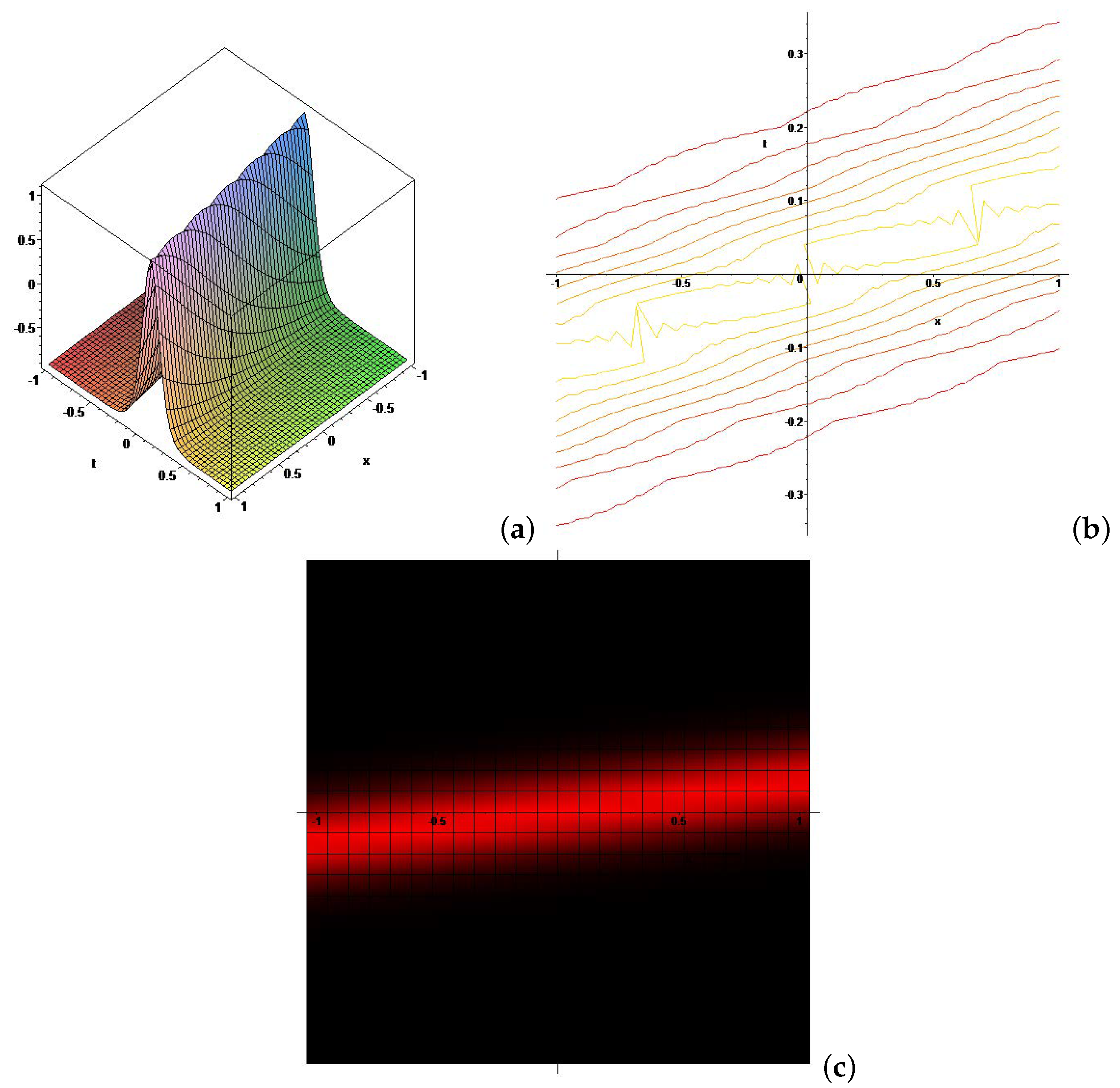
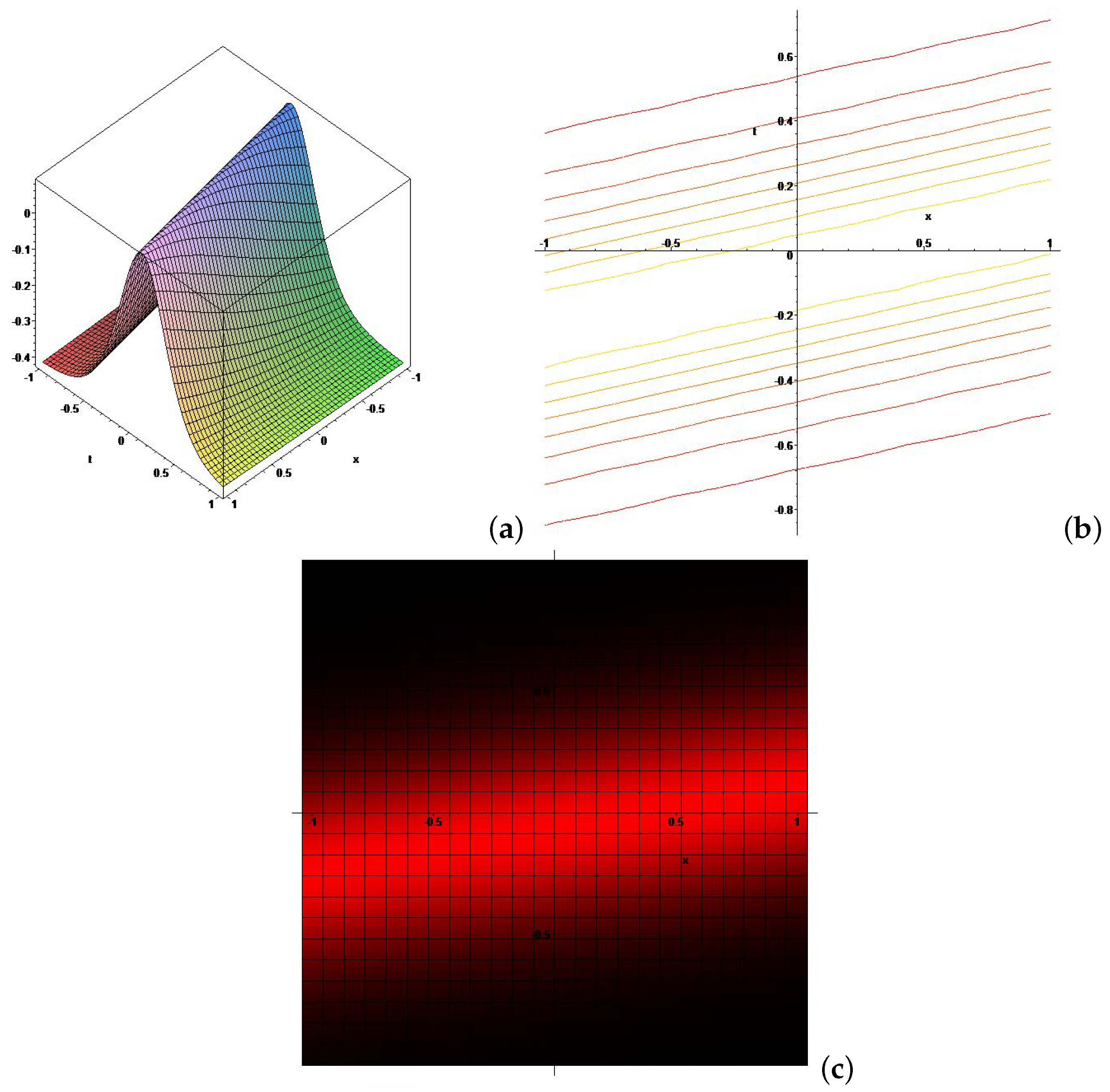
4. Graphical Representations

In this section, we will provide visual depictions illustrating the results acquired in the previous section (Figure 1 and Figure 2).

5. Conclusions

The current paper conducted additional investigation on new analytical solutions to the extended (3 + 1)-dimensional Sakovich equation. In this article, seven different types of solutions originated via the GERFM. The applied solutions differ from the results obtained through previously employed methods [25,26,27]. The physical characteristics of the generated solutions have been examined through graphical representations. Arbitrary parameters are included in the solutions, and different solutions can be built by setting the parameters to different values. The graphical representations are given by setting $\alpha =\beta =\gamma =1$ and $y=z=0$. The solutions obtained are inventive and novel, not previously documented in existing papers, and hold significant value in characterizing nonlinear physical structures. The Maple software program was employed for simulating and analyzing the results. It is critical to note that the accuracy of the solutions was validated through their substitution into the equation.

References

1. Seadawy, A.R.; Arshad, M.; Lu, D. The weakly nonlinear wave propagation theory for the Kelvin-Helmholtz instability in magnetohydrodynamics flows, Chaos. Solitons Fractals 2020, 139, 110141. [Google Scholar] [CrossRef]
2. Raza, N.; Abdel-Aty, A.H. Traveling wave structures and analysis of bifurcation and chaos theory for Biswas-Milovic Model in conjunction with Kudryshov’s law of refractive index. Optik 2023, 287, 171085. [Google Scholar] [CrossRef]
3. Cheng, L.; Ma, W.X. Similarity Transformations and Nonlocal Reduced Integrable Nonlinear Schrödinger Type Equations. Mathematics 2023, 11, 4110. [Google Scholar] [CrossRef]
4. Ma, W.X.; Batwa, S.; Manukure, S. Dispersion-Managed Lump Waves in a Spatial Symmetric KP Model. East Asian J. Appl. Math. 2023, 13, 246–256. [Google Scholar] [CrossRef]
5. Raza, N.; Deifalla, A.; Rani, B.; Shah, N.A.; Ragab, A.E. Analyzing Soliton Solutions of the (n+1)-dimensional generalized Kadomtsev-Petviashvili equation: Comprehensive study of dark, bright, and periodic dynamics. Results Phys. 2024, 56, 107224. [Google Scholar] [CrossRef]
6. Malfliet, W. Solitary wave solutions of nonlinear wave equations. Am. J. Phys. 1992, 60, 650–654. [Google Scholar] [CrossRef]
7. Rizvi, S.T.R.; Seadawy, A.R.; Alsallami, S.A.M. Grey-Black Optical Solitons, Homoclinic Breather, Combined Solitons via Chupin Liu’s Theorem for Improved Perturbed NLSE with Dual-Power Law Nonlinearity. Mathematics 2023, 11, 2122. [Google Scholar] [CrossRef]
8. Taghizadeh, N.; Mirzazadeh, M.; Tascan, F. The first-integral method applied to the Eckhaus equation. Appl. Math. Lett. 2012, 25, 798–802. [Google Scholar] [CrossRef]
9. Mishaev, R.A. Auto-Bäcklund transformations for the nonlinear Schrödinger equation with variable coefficients. Theor. Math. Phys. 1995, 102, 144–152. [Google Scholar] [CrossRef]
10. Kemaloglu, B.; Yel, G.; Bulut, H. An application of the rational sine-Gordon method to the Hirota equation. Opt. Quantum Electron. 2023, 55, 658. [Google Scholar] [CrossRef]
11. Alam, M.N.; Ilhan, O.A.; Manafian, J.; Asjad, M.I.; Rezazadeh, H.; Baskonus, H.M. New Results of Some of the Conformable Models Arising in Dynamical Systems. Adv. Math. Phys. 2022, 2022, 7753879. [Google Scholar] [CrossRef]
12. Inc, M.; Alqahtani, R.T.; Iqbal, M.S. Stability analysis and consistent solitary wave solutions for the reaction-diffusion regularized nonlinear model. Results Phys. 2023, 54, 107053. [Google Scholar] [CrossRef]
13. Malik, S.; Hashemi, M.S.; Kumar, S.; Rezazadeh, H.; Mahmoud, W.; Osman, M.S. Application of new Kudryashov method to various nonlinear partial differential equations. Opt. Quantum Electron. 2023, 55, 8. [Google Scholar] [CrossRef]
14. Akbulut, A.; Tascan, F.; Ozel, E. Trivial conservation laws and solitary wave solution of the fifth order Lax equation. Partial Differ. Appl. Math. 2021, 4, 100101. [Google Scholar] [CrossRef]
15. Akbulut, A.; Rezazadeh, H.; Hashemi, M.S.; Tascan, F. The (3 + 1)-dimensional Wazwaz-KdV equations: The conservation laws and exact solutions. Int. J. Nonlinear Sci. Numer. 2023, 24, 673–693. [Google Scholar] [CrossRef]
16. Liu, S.K.; Fu, Z.; Liu, S.D.; Zhao, Q. Jacobi elliptic function method and periodic wave solutions of nonlinear wave equations. Phys. Lett. A 2001, 289, 69–74. [Google Scholar] [CrossRef]
17. Yang, X.F.; Deng, Z.C.; Wei, Y. A Riccati-Bernoulli sub-ODE method for nonlinear partial differential equations and its application. Adv. Differ. Equ. 2015, 117. [Google Scholar] [CrossRef]
18. Humbu, I.; Muatjetjeja, B.; Motsumi, T.G.; Adem, A. Solitary waves solutions and local conserved vectors for extended quantum Zakharov-Kuznetsov equation. Eur. Phys. J. Plus 2023, 138, 873. [Google Scholar] [CrossRef]
19. Wazwaz, A.M.; Hammad, M.A.; Al-Ghamdi, A.O.; Alshehri, M.H.; El-Tantawy, S.A. New (3 + 1)-Dimensional Kadomtsev-Petviashvili-Sawada-Kotera-Ramani Equation: Multiple-Soliton and Lump Solutions. Mathematics 2023, 11, 3395. [Google Scholar] [CrossRef]
20. Sakovich, S. A new Painlevé-integrable equation possessing KdV-type solitons. arXiv 2019, arXiv:1907.01324. [Google Scholar]
21. Wazwaz, A.M. A new (3 + 1)-dimensional Painlevé-integrable Sakovich equation: Multiple soliton solutions. Int. J. Numer. Methods Heat Fluid Flow 2021, 31, 3030–3035. [Google Scholar] [CrossRef]
22. Singh, S.; Ray, S.S. Painlevé analysis, auto-Bäcklund transformation and new exact solutions of (2+1) and (3 + 1)-dimensional extended Sakovich equation with time dependent variable coefficients in ocean physics. J. Ocean Eng. Sci. 2023, 8, 246–262. [Google Scholar] [CrossRef]
23. Wazwaz, A.M. Two new Painlevé-integrable extended Sakovich equations with (2+1) and (3 + 1) dimensions. Int. J. Numer. Methods Heat Fluid Flow 2020, 30, 1379–1387. [Google Scholar] [CrossRef]
24. Younis, M.; Seadawy, A.R.; Baber, M.Z.; Yasin, M.W.; Rizvi, S.T.; Iqbal, M.S. Abundant solitary wave structures of the higher dimensional Sakovich dynamical model. Math. Methods Appl. Sci. 2021. [Google Scholar] [CrossRef]
25. Ma, Y.L.; Wazwaz, A.M.; Li, B.Q. A new (3 + 1)-dimensional Sakovich equation in nonlinear wave motion: Painlevé integrability, multiple solitons and soliton molecules. Qual. Theory Dyn. Syst. 2022, 21, 158. [Google Scholar] [CrossRef]
26. Ali, K.K.; AlQahtani, S.A.; Mehanna, M.S.; Wazwaz, A.M. Novel soliton solutions for the (3 + 1)-dimensional Sakovich equation using different analytical methods. J. Math 2023, 2023, 4864334. [Google Scholar] [CrossRef]
27. Cortez, M.V.; Raza, N.; Kazmi, S.S.; Chahlaoui, Y.; Basendwah, G.A. A novel investigation of dynamical behavior to describe nonlinear wave motion in (3 + 1)-dimensions. Results Phys. 2023, 55, 107131. [Google Scholar] [CrossRef]
28. Ghanbari, B.; Inc, M.; Yusuf, A.; Bayram, M. Exact optical solitons of Radhakrishnan-Kundu-Lakshmanan equation with Kerr law nonlinearity. Mod. Phys. Lett. B 2019, 33, 1950061. [Google Scholar] [CrossRef]
29. Gunay, B.; Kuo, C.K.; Ma, W.X. An application of the exponential rational function method to exact solutions to the Drinfeld-Sokolov system. Results Phys. 2021, 29, 104733. [Google Scholar] [CrossRef]
Figure 1. (a) A 3D graph depicting Equation (26). (b) A contour plot depicting Equation (26). (c) A density plot depicting Equation (26).
Mathematics 12 00720 g001
Figure 2. (a) A 3D graph depicting Equation (32). (b) A contour plot depicting Equation (32). (c) A density plot depicting Equation (32).
Mathematics 12 00720 g002
Disclaimer/Publisher’s Note: The statements, opinions and data contained in all publications are solely those of the individual author(s) and contributor(s) and not of MDPI and/or the editor(s). MDPI and/or the editor(s) disclaim responsibility for any injury to people or property resulting from any ideas, methods, instructions or products referred to in the content.