Simulation of a Combined (2+1)-Dimensional Potential Kadomtsev–Petviashvili Equation via Two Different Methods

Abstract

This paper presents an investigation into original analytical solutions of the (2+1)-dimensional combined potential Kadomtsev–Petviashvili and B-type Kadomtsev–Petviashvili equations. For this purpose, the generalized Kudryashov technique (GKT) and exponential rational function technique (ERFT) have been applied to deal with the equation. These two methods have been applied to the model for the first time, and the the generalized Kudryashov method has an important place in the literature. The characteristics of solitons are unveiled through the use of three-dimensional, two-dimensional, contour, and density plots. Furthermore, we conducted a stability analysis on the acquired results. The results obtained in the article were seen to be different compared to other results in the literature and have not been published anywhere before.

1. Introduction

In recent years, there has been an increasing interest in the quest for exact solutions within the domain of nonlinear partial differential equations (NPDEs). Exact solutions are solutions to mathematical equations that can be expressed in a closed form, meaning they can be written as a formula or as an explicitly defined function. Exact solutions are valuable for several reasons; for example, they provide insights into the underlying behavior of the equations. By analyzing the form of an exact solution, we can gain a deeper understanding of the phenomena described by the equations, and they can be used to validate approximate solutions. If an approximate solution agrees with an exact solution, we can be more confident in its accuracy and it can be used to make predictions about real-world phenomena. In some cases, exact solutions can be used to make predictions about the behavior of physical systems.

Exact solutions have been used to study a wide range of phenomena; for example, Einstein’s field equations, which describe the curvature of spacetime, have exact solutions that describe the motion of planets and stars; the Navier–Stokes equations, which describe the flow of fluids, have exact solutions that can be used to study the behavior of fluids in various situations; and the equations of elasticity and plasticity, which describe the behavior of materials under stress, have exact solutions that can be used to study the deformation of materials. The study of exact solutions is an active area of research, and new exact solutions are being discovered all the time. These solutions provide valuable insights into the behavior of complex systems and can be used to make predictions about the behavior of real-world phenomena.

The examination of solutions of these equations has become crucial across various fields of science and technology, including control theory, fiber optics, solid-state mechanics, transport infrastructure, atomic engineering, fluid dynamics, and various other research fields. Numerous successful approaches have been devised for investigating dynamic structures, such as lump solutions [1,2], the matrix eigenvalue problem [3], auto-Backlund transformations [4], the auxiliary equation method [5], the generalized Riccati equation mapping technique [6], the addendum to the Kudryashov technique [7], the unified method [8], the modified extended tanh-function approach [9], the Hirota bilinear technique [10], the Lie symmetry approach [11], the improved Bernoulli sub-equation function procedure [12], the modified ($G^{\prime }/G$)-expansion method [13], the bilinear method [14], an extended ($G^{\prime }/G$)-expansion method [15], the tanh–coth method [16,17], and so on.

In this research, our objective is to investigate a (2+1)-dimensional combined potential Kadomtsev–Petviashvili equation incorporating the B-type Kadomtsev–Petviashvili (pKP-BKP) equation:

$$\begin{array}{c}{b}_1(45u_x^2{u}_{xx}+15u_{xx}{u}_{3x}+15u_x{u}_{4x}+u_{6x})+b_2(6u_x{u}_{xx}+u_{4x})\\ +b_3(3u_x{u}_{xy}+3u_{xx}{u}_y+u_{3xy})+b_4{u}_{xx}+b_5{u}_{xt}+b_6{u}_{yy}=0.\end{array}$$

(1)

where we can choose b as a function of x in some formulations of the KP-pKPBKP equation. This choice can introduce spatial variation into the strength of internal wave effects, leading to more intricate wave dynamics and patterns. The equation introduced by Ma in [18] denoted as Equation (1) has been demonstrated to possess an N-soliton solution. Ma provided a comprehensive analysis of this equation, where the parameters $b_i(i=1,\dots ,6)$ are constants capable of influencing the amplitude, depth, width, and periodicity of the associated wave with arbitrary values. The spatial dimensions are represented by x and y, while u signifies the amplitude of the relevant wave and t corresponds to time. This equation exhibits versatility as it can be transformed into various other nonlinear equations, each manifesting distinct physical characteristics. Specifically, when $b_1=b_3=b_4=0,$ $b_2=b_5=1$, and $b_6=-1$, Equation (1) reduces to a (2+1)-dimensional potential Kadomtsev–Petviashvili (pKP) equation. The derived pKP equation models the dynamics of a wave and is expressed as follows:

$$6u_x{u}_{xx}+u_{4x}+u_{xt}-u_{yy}=0.$$

When $b_1=b_5=1,b_2=b_4=0,b_3=5$, and $b_6=-5$, Equation (1) undergoes a transformation into a (2+1)-dimensional B-type Kadomtsev–Petviashvili (BKP) equation. This BKP equation serves as a valuable physical model and can be expressed as follows:

$$45u_x^2{u}_{xx}+15u_{xx}{u}_{3x}+15u_x{u}_{4x}+u_{6x}+5(3u_x{u}_{xy}+3u_{xx}{u}_y+u_{3xy})+u_{xt}-5u_{yy}=0$$

Recently, several researchers have explored Equation (1) employing diverse approaches. For instance, Ma et al. delved into the precise solutions of Equation (1) utilizing the Hirota bilinear method [19], while Feng et al. acquired resonant multi-soliton solutions through the application of the linear superposition principle [20]. In contrast to previous investigations, we will apply two different methods to find original analytical solutions, namely the generalized Kudryashov technique and the exp rational function method, and we will present a stability analysis of the obtained results. The aim of this paper is to obtain exact solutions of the (2+1)-dimensional combined potential Kadomtsev–Petviashvili equation via two different methods, which are the GKT and ERFT methods, and to search for the stability of some of the obtained solutions. For this purpose, Section 2 provides a brief description of the GKT and ERFT. Thereafter, in Section 3, we utilize the mentioned methods on the (2+1)-dimensional B-type Kadomtsev–Petviashvili (BKP) equation. A stability analysis and visual representations of the obtained results are given in Section 4. Finally, Section 5 provides the conclusions of the paper.

2. Methodology

This section provides a detailed explanation of the GKT and ERFT.

2.1. The Generalized Kudryashov Technique

Within this section, we introduce the GKT to find exact solutions of NPDEs [21,22,23,24].

We examine a general NPDE presented as:

$$P(u,u_x,u_y,u_t,u_{xx},u_{yy},\dots )=0,$$

(2)

where P is a polynomial of $u(x,y,t)$ and its partial derivatives, in which the highest order derivatives and nonlinear terms are involved.

The main steps of the GKT are as follows:

Step 1: We use the wave transformation to transform the nonlinear partial differential equation into an ordinary differential equation, and this transformation comes from Lie symmetries. In the search for a traveling wave solution of the equation, we apply the traveling wave transformation:

$$\xi =x+y-ct$$

(3)

By using Equation (3), Equation (2) reduces to a nonlinear ordinary differential equation (ODE).

$$H(u,u^{\prime },u^{″},\dots ,)=0,$$

(4)

where the prime denotes derivation with respect to $\xi$.

Step 2: Assume that the solution to Equation (4) can be expressed in the subsequent rational form:

$$u\left(\xi \right)=\frac{{\displaystyle \sum _{i=0}^N}{\alpha }_i{R}^i\left(\xi \right)}{{\displaystyle \sum _{j=0}^M}{\beta }_j{R}^j\left(\xi \right)}$$

(5)

where ${\alpha }_i(i=0,1,\dots ,N),{\beta }_j(j=0,1,\dots ,M)$ are constants to be determined such that ${\alpha }_N\ne 0$, ${\beta }_M\ne 0$ and $R=R\left(\xi \right)$ satisfies the ODE

$$\frac{dR}{d\xi }=R^2\left(\xi \right)-R\left(\xi \right)$$

(6)

It is obvious that the solution of Equation (6) is

$$R\left(\xi \right)=\frac{1}{1+A{e}^{\xi }}$$

(7)

where A is an integration constant.

Step 3: To obtain the positive integers N and M in Equation (5) through the application of the homogeneous balance method, the relationship between the highest-order derivatives and the highest-power nonlinear terms in Equation (4) is considered.

Step 4: By substituting Equation (5) into Equation (4) along with Equation (6), we derive a polynomial in terms of $R\left(\xi \right)$. Next, by setting all coefficients of $R\left(\xi \right)$ to zero, we establish a system of algebraic equations. Utilizing Maple, we can solve this system to determine the values of ${\alpha }_i(i=0,1,\dots ,N),{\beta }_j(j=0,1,\dots ,M).$ Finally, if we substitute these values and Equation (6) into Equation (5), we can obtain the precise solutions for the reduced (4).

2.2. The Exponential Rational Function Technique (ERFT)

In the literature, some methods, such as the new generalized exponential rational function method [25] and the new modification of the exponential rational function method [26], give more general forms of the solutions.

Step 1.

The solution of Equation (4) can be expressed as follows [27]:

$$u\left(\xi \right)=\sum _{n=0}^N\frac{{\eta }_n}{{(1+e^{\xi })}^n},$$

(8)

where ${\eta }_n$$\left({\eta }_N\ne 0\right)$ are constants to be determined later. Determine the integer N by the homogenous balance method. This method consists of balancing the highest-order linear term with the highest-order nonlinear term in Equation (4).

Step 2.

Putting Equation (8) into Equation (4) and separating all terms with the same order of $e^{n\xi }$$(n=0,1,2,\dots )$, we convert the left-hand side of Equation (4) into another polynomial in $e^{n\xi }$. Then, we equate each coefficient of this polynomial to zero, yielding a set of algebraic equations for ${\eta }_n$ unknown parameters. Finally, we solve the equation system to construct a variety of exact solutions for Equation (2).

3. Implementations

This section provides the (2+1)-dimensional combined potential Kadomtsev–Petviashvili and B-type Kadomtsev–Petviashvili equations. For this purpose, first of all, applying the transformation Equation (3) to Equation (1) yields the following ordinary differential equation:

$$\begin{array}{c}{b}_1(45{\left(u^{\prime }\right)}^2{u}^{″}+15u^{″}{u}^{\left(3\right)}+15u^{\prime }{u}^{\left(4\right)}+u^{\left(6\right)})+b_2(6u^{\prime }{u}^{″}+u^{\left(4\right)})\hfill \\ +b_3(3u^{\prime }{u}^{″}+3u^{″}{u}^{\prime }+u^{\left(4\right)})+b_4{u}^{″}-b_{5}c{u}^{″}+b_6{u}^{″}=0.\hfill \end{array}$$

(9)

If we integrate this equation once with respect to $\xi$, we find:

$$\begin{array}{c}15b_1{\left(u^{\prime }\right)}^3+3{\left(u^{\prime }\right)}^2(b_2+b_3)-b_{5}c{u}^{\prime }+(b_4+b_6)u^{\prime }\hfill \\ +b_1\left(15u^{\prime }+\frac{b_2}{b_1}+\frac{b_3}{b_1}\right)u^{‴}+b_1{u}^{\left(5\right)}=0.\hfill \end{array}$$

(10)

3.1. Implementation of the GKT to the Combined (2+1)-Dimensional Potential Kadomtsev–Petviashvili and B-Type Kadomtsev–Petviashvili Equations

By employing the homogeneous balance principle in Equation (10), we derive the balancing number as $N=M+1$. Setting M to 1 leads to the determination of N as 2. Consequently, the solution can be formulated as follows:

$$u\left(\xi \right)=\frac{{\alpha }_0+{\alpha }_{1}R+{\alpha }_2{R}^2}{{\beta }_0+{\beta }_{1}R},$$

(11)

Here, $R\left(\xi \right)$ represents Equation (7). Considering this, Equation (11) will be substituted into Equation (9). Thereafter, we equate all coefficients of the functions $R\left(\xi \right)$ to zero, resulting in a system of equations. This system is given in the appendix (see Appendix A). From the solutions of this system, we identify several scenarios that are subsequently discussed in detail as follows:

Case 1:

$$\begin{array}{c}{\alpha }_0=-\frac{{\alpha }_1}{2},{\alpha }_1={\alpha }_1,{\alpha }_2=-2{\beta }_1,\hfill \\ \\ {\beta }_0=-\frac{{\beta }_1}{2},{\beta }_1={\beta }_1,c=\frac{4b_3+16b_1+4b_2+b_4+b_6}{b_5}\hfill \end{array}$$

Therefore, the analytical solution of the (2+1)-dimensional combined potential Kadomtsev–Petviashvili and B-type Kadomtsev–Petviashvili equations is given as:

$$u(x,y,t)=\frac{-\frac{{\alpha }_1}{2}+\frac{{\alpha }_1}{B_1(x,y,t)}-\frac{2{\beta }_1}{B_1^2(x,y,t)}}{-\frac{{\beta }_1}{2}+\frac{{\beta }_1}{B_1(x,y,t)}},$$

(12)

where $B_1(x,y,t)=1+A\left(cosh\left(x+y-\frac{4b_3+16b_1+4b_2+b_4+b_6}{b_5}t\right)+sinh\left(x+y-\frac{4b_3+16b_1+4b_2+b_4+b_6}{b_5}t\right)\right)$ and A is an integration constant.

Case 2:

$$\begin{array}{c}{\alpha }_0=\frac{{\beta }_0({\alpha }_1+2{\beta }_0)}{{\beta }_1},{\alpha }_1={\alpha }_1,{\alpha }_2=-2{\beta }_1,\hfill \\ c=\frac{b_4+b_2+b_3+b_6+b_1}{b_5},\hfill \\ {\beta }_0={\beta }_0,{\beta }_1={\beta }_1,\hfill \end{array}$$

Therefore, the analytical solution of the (2+1)-dimensional combined potential Kadomtsev–Petviashvili and B-type Kadomtsev–Petviashvili equations is given as:

$$u(x,y,t)=\frac{\frac{{\beta }_0({\alpha }_1+2{\beta }_0)}{{\beta }_1}+\frac{{\alpha }_1}{B_2(x,y,t)}-\frac{2{\beta }_1}{B_2^2(x,y,t)}}{{\beta }_0+\frac{{\beta }_1}{B_2(x,y,t)}},$$

(13)

where $B_2(x,y,t)=1+A\left(cosh\left(x+y-\frac{b_4+b_2+b_3+b_6+b_1}{b_5}t\right)+sinh\left(x+y-\frac{b_4+b_2+b_3+b_6+b_1}{b_5}t\right)\right)$ and A is an integration constant.

3.2. Implementation of the ERFT to the Combined (2+1)-Dimensional Potential Kadomtsev–Petviashvili and B-Type Kadomtsev–Petviashvili Equations

By employing the homogeneous balance principle in Equation (10), we derive the balancing number as $N=1.$ Therefore, the solution will take the following form:

$$u\left(\xi \right)={\eta }_0+\frac{{\eta }_1}{1+e^{\xi }}$$

(14)

When we insert this equation into Equation (10), we discover the ensuing system of equations as follows:

$$\begin{array}{ccc}{e}^{5\xi }\hfill & :\hfill & b_{5}c{\eta }_1-b_3{\eta }_1-b_1{\eta }_1-b_2{\eta }_1-b_6{\eta }_1-b_4{\eta }_1=0,\hfill \\ \hfill & \hfill & \\ e^{4\xi }\hfill & :\hfill & 3b_3{\eta }_1^2+3b_2{\eta }_1^2+15b_1{\eta }_1^2+2b_3{\eta }_1+2b_2{\eta }_1-4b_4{\eta }_1\hfill \\ \hfill & \hfill & -4b_6{\eta }_1+4b_{5}c{\eta }_1+26b_1{\eta }_1=0,\hfill \\ \hfill & \hfill & \\ e^{3\xi }\hfill & :\hfill & -60b_1{\eta }_1^2-6b_6{\eta }_1+6b_2{\eta }_1-15{\eta }_1^3{b}_1+6b_2{\eta }_1^2-66b_1{\eta }_1\hfill \\ \hfill & \hfill & +6b_{5}c{\eta }_1+6b_3{\eta }_1^2+6b_3{\eta }_1-6b_4{\eta }_1=0,\hfill \\ \hfill & \hfill & \\ e^{2\xi }\hfill & :\hfill & 3b_3{\eta }_1^2+3b_2{\eta }_1^2+15b_1{\eta }_1^2+2b_3{\eta }_1+2b_2{\eta }_1-4b_4{\eta }_1\hfill \\ \hfill & \hfill & -4b_6{\eta }_1+4b_{5}c{\eta }_1+26b_1{\eta }_1=0,\hfill \\ \hfill & \hfill & \\ e^{\xi }\hfill & :\hfill & b_{5}c{\eta }_1-b_3{\eta }_1-b_1{\eta }_1-b_2{\eta }_1-b_6{\eta }_1-b_4{\eta }_1=0\hfill \end{array}$$

By solving this system, the following outcomes are generated:

$${\eta }_1=-2,c=\frac{b_1+b_2+b_3+b_4+b_6}{b_5}.$$

(15)

Therefore, the analytical solution of the (2+1)-dimensional combined potential Kadomtsev–Petviashvili and B-type Kadomtsev–Petviashvili equations can be given as

$$u(x,y,t)={\eta }_0-\frac{2}{1+cosh\left(x+y-\left(\frac{b_1+b_2+b_3+b_4+b_6}{b_5}\right)t\right)+sinh\left(x+y-\left(\frac{b_1+b_2+b_3+b_4+b_6}{b_5}\right)t\right)}.$$

(16)

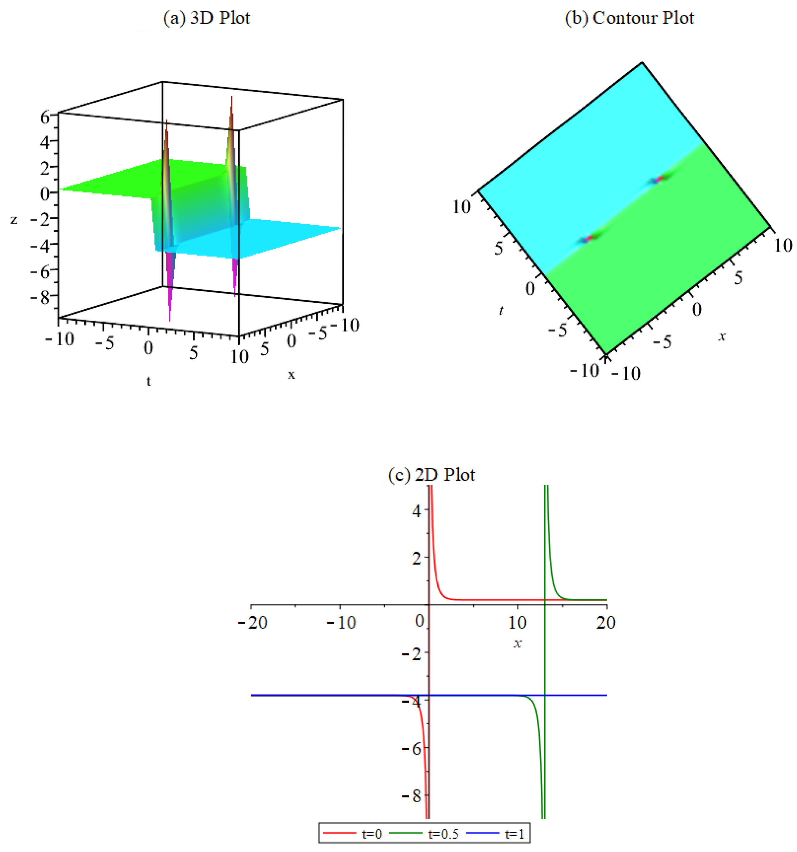
4. Stability Analysis and Graphical Representations

In this section, we will present the plots of the results. Plots will be given in three dimensions, in two dimensions, and as contour figures. In two-dimensional figures, a red line was drawn when $t=0$, a green line was drawn when $t=0.5$, and a blue line was drawn when $t=1.$ Figure 1 represents the periodic solution shape for Equation (12).

Figure 2 represents the kink solution shape for Equation (13).

Figure 3 represents the kink solution shape for Equation (16).

A solution to a differential equation is called stable if small perturbations in the initial conditions lead to solutions that remain close to the original solution. This is relevant in various fields like physics, engineering, and economics. The stability property of the solutions is closely related to the momentum in a Hamilton system. From this point of view, the following formula is given for the Hamiltonian system of the solution:

$${\Psi }_H=\frac{1}{2}{\int }_{-ϵ}^{ϵ}{u}^2\left(\xi \right)d\xi ,$$

where $u\left(\xi \right)$ is the solution of the model. Then, we calculate the momentum of the Hamilton system as follows:

$$\frac{\partial \Psi }{\partial c}{\mid }_{c=\sigma }>0,$$

where $\sigma$ is an optional constant [28,29].

Assuming the values of the constants ${\alpha }_1=1,{\beta }_1=1,y=1,A=1,c=2$ in Equation (12), and considering the solution in the square area of $\left[-2,2\right]$ and performing the necessary operations, we find the condition as follows:

$$\frac{\partial \Psi }{\partial c}{\mid }_{c=2}=9.029945870-6.283185305I.$$

According to the above result, our solution is stable for the assumed conditions.

Assuming the values of the constants ${\alpha }_1=1,{\beta }_0=1,{\beta }_1=1,y=1,A=1,c=2$ in Equation (13), and considering the solution in the square area of $\left[-2,2\right]$ and performing the necessary operations, we find the condition as follows:

$$\frac{\partial \Psi }{\partial c}{\mid }_{c=2}=-1.475503757.$$

According to the above result, our solution is unstable for the assumed conditions.

Assuming the values of the constants ${\eta }_0=1,c=2$ in Equation (16), and considering the solution in the square area of $\left[-2,2\right]$ and performing the necessary operations, we find the condition as follows:

$$\frac{\partial \Psi }{\partial c}{\mid }_{c=2}=1.205362104.$$

According to the above result, our solution is stable for the assumed conditions.

5. Conclusions

In our paper, we have effectively obtained explicit solutions for traveling wave patterns for the (2+1)-dimensional combined potential Kadomtsev–Petviashvili and B-type Kadomtsev–Petviashvili equations employing direct methods through the GKT and ERFT. These two methods have been applied to the model for the first time, and the generalized Kudryashov method has an important place in the literature. When we compared our results with the existing literature, we identified a variety of solutions, each demonstrating a unique behavior. We conducted an analysis of stability and provided visual representations, including 2D, 3D, and contour plots of the obtained solutions. Our results exhibit distinctions from those present in the existing literature, characterized by the inclusion of a multitude of arbitrary constants, yielding a comprehensive array of solutions. In addition, we have enriched our paper with a stability analysis and graphical representations. The importance of the figures lies in discerning the configurations of the acquired wave solutions, with each figure defining a specific type of wave solution. Graphical representations are instrumental in understanding wave motions. The capacity to determine solutions holds significance across various fields, including mathematics, physics, and, notably, fiber optics. The research techniques employed in this study can be extended to a broad spectrum of nonlinear dynamical models encountered in diverse engineering and scientific disciplines.

References

1. Lu, X.; Ma, W.X. Study of lump dynamics based on a dimensionally reduced Hirota bilinear equation. Nonlinear Dyn. 2016, 85, 1217–1222. [Google Scholar] [CrossRef]
2. Ismael, H.F.; Nabi, H.R.; Sulaiman, T.A.; Shah, N.A.; Eldin, S.M.; Bulut, H. Hybrid and physical interaction phenomena solutions to the Hirota bilinear equation in shallow water waves theory. Results Phys. 2023, 53, 106978. [Google Scholar] [CrossRef]
3. Ma, W.X. Reduced Non-Local Integrable NLS Hierarchies by Pairs of Local and Non-Local Constraints. Int. J. Comput. 2022, 8, 206. [Google Scholar] [CrossRef]
4. Kaplan, M.; Ozer, M.N. Auto-Bäcklund transformations and solitary wave solutions for the nonlinear evolution equation. Opt. Quantum Electron. 2018, 50, 33. [Google Scholar] [CrossRef]
5. Ray, S.S. New Soliton and Periodic Wave Solutions to the Fractional DGH Equation Describing Water Waves in a Shallow Regime. Qual. Theory Dyn. Syst. 2022, 21, 151. [Google Scholar]
6. Kumar, S.; Kumar, A. Newly generated optical wave solutions and dynamical behaviors of the highly nonlinear coupled Davey-Stewartson Fokas system in monomode optical fibers. Opt. Quantum Electron. 2023, 55, 566. [Google Scholar] [CrossRef]
7. Alotaibi, H. Explore Optical Solitary Wave Solutions of the kp Equation by Recent Approaches. Crystals 2022, 12, 159. [Google Scholar] [CrossRef]
8. Raza, N.; Seadawy, A.R.; Salman, F. Extraction of new optical solitons in presence of fourth-order dispersion and cubic-quintic nonlinearity. Opt. Quantum Electron. 2023, 55, 370. [Google Scholar] [CrossRef]
9. Akbulut, A.; Kaplan, M.; Kaabar, M.K.A. New exact solutions of the Mikhailov-Novikov-Wang equation via three novel techniques. J. Ocean. Eng. Sci. 2023, 8, 103–110. [Google Scholar] [CrossRef]
10. Hosseini, K.; Salahshour, S.; Baleanu, D.; Mirzazadeh, M.; Dehingia, K. A new generalized KdV equation: Its lump-type, complexiton and soliton solutions. Int. J. Mod. Phys. 2022, 36, 2250229. [Google Scholar] [CrossRef]
11. Cortez, M.V.; Raza, N.; Kazmi, S.S.; Chahlaoui, Y.; Basendwah, G.A. A novel investigation of dynamical behavior to describe nonlinear wave motion in (3+1)-dimensions. Results Phys. 2023, 55, 107131. [Google Scholar] [CrossRef]
12. Haque, M.M.; Akbar, M.A.; Rezazadeh, H.; Bekir, A. A variety of optical soliton solutions in closed-form of the nonlinear cubic quintic Schrödinger equations with beta derivative. Opt. Quantum Electron. 2023, 55, 1144. [Google Scholar] [CrossRef]
13. Alam, M.N.; Islam, S.; Ilhan, O.A.; Bulut, H. Some new results of nonlinear model arising in incompressible visco-elastic Kelvin-Voigt fluid. Math. Meth. Appl. Sci. 2022, 45, 10347–10362. [Google Scholar] [CrossRef]
14. Sun, Y.; Hu, Z.; Triki, H.; Mirzazadeh, M.; Liu, W.; Biswas, A.; Zhou, Q. Analytical study of three-soliton interactions with different phases in nonlinear optics. Nonlinear Dyn. 2023, 111, 18391–18400. [Google Scholar] [CrossRef]
15. Kumar, V.; Gupta, R.K.; Jiwari, R. Lie group analysis, numerical and non-traveling wave solutions for the (2+1)-dimensional diffusion-advection equation with variable coefficients. Chin. Phys. B 2014, 23, 030201. [Google Scholar] [CrossRef]
16. Kumar, S.; Jiwari, R.; Mittal, R.C.; Awrejcewicz, J. Dark and bright soliton solutions and computational modeling of nonlinear regularized long wave model. Nonlinear Dyn. 2021, 104, 661–682. [Google Scholar] [CrossRef]
17. Jiwari, A.R. New multiple analytic solitonary solutions and simulation of (2+1)-dimensional generalized Benjamin-Bona-Mahony-Burgers model. Nonlinear Dyn. 2023, 111, 13297–13325. [Google Scholar]
18. Ma, W.X. N-soliton solution of a combined pkp-bkp equation. J. Geom. Phys. 2021, 165, 104191. [Google Scholar] [CrossRef]
19. Ma, Z.Y.; Fei, J.X.; Cao, W.P.; Wu, H.L. The explicit solution and its soliton molecules in the (2+1)-dimensional pkp-bkp equation. Results Phys. 2022, 35, 105363. [Google Scholar] [CrossRef]
20. Feng, Y.; Bilige, S. Resonant multi-soliton, m-breather, m-lump and hybrid solutions of a combined pkp-bkp equation. J. Geom. Phys. 2021, 169, 104322. [Google Scholar] [CrossRef]
21. Kudryashov, N.A. Solitary and periodic waves of the hierarchy for propagation pulse in optical fiber. Optik 2019, 194, 163060. [Google Scholar] [CrossRef]
22. Kudryashov, N.A. One method for finding exact solutions of nonlinear differential equations. Commun. Nonlinear Sci. Numer. Simul. 2012, 17, 2248–2253. [Google Scholar] [CrossRef]
23. Habib, M.A.; Ali, H.M.S.; Miah, M.M.; Akbar, M.A. The generalized Kudryashov method for new closed form traveling wave solutions to some NLEEs. Aims Math. 2019, 4, 896–909. [Google Scholar] [CrossRef]
24. Ekici, M. Exact Solutions to Some Nonlinear Time-Fractional Evolution Equations Using the Generalized Kudryashov Method in Mathematical Physics. Symmetry 2023, 15, 1961. [Google Scholar] [CrossRef]
25. Ghanbari, B.; Inc, M. A new generalized exponential rational function method to find exact special solutions for the resonance nonlinear Schrödinger equation. Eur. Phys. J. Plus 2018, 133, 142. [Google Scholar] [CrossRef]
26. Ahmed, N.; Bibi, S.; Khan, U.; Mohyud-Din, S.T. A new modification in the exponential rational function method for nonlinear fractional differential equations. Eur. Phys. J. Plus 2018, 133, 45. [Google Scholar] [CrossRef]
27. Bekir, A.; Kaplan, M. Exponential rational function method for solving nonlinear equations arising in various physical models. Chin. J. Phys. 2016, 54, 365–370. [Google Scholar] [CrossRef]
28. Yue, C.; Khater, M.M.A.; Attia, R.A.M.; Lu, D. The plethora of explicit solutions of the fractional KS equation through liquid–gas bubbles mix under the thermodynamic conditions via Atangana–Baleanu derivative operator. Adv. Differ. Equ. 2020, 2020, 62. [Google Scholar] [CrossRef]
29. Sedawy, A.R.; Lu, D.; Yue, C. Travelling wave solutions of the generalized nonlinear fifth-order KdV water wave equations and its stability. J. Taibah Univ. Sci. 2017, 11, 623–633. [Google Scholar] [CrossRef]
Figure 1. Plots of Equation (12) when y = 0 , α 1 = 0.1 , β 1 = b 1 = b 2 = b 3 = b 4 = b 5 = b 6 = 0.5 , A = 1.
Mathematics 12 00427 g001
Figure 2. Plots of Equation (13) when y = 0 , α 1 = β 0 = β 1 = b 1 = b 2 = b 3 = b 4 = b 5 = b 6 = 0.5 , A = 1 .
Mathematics 12 00427 g002aMathematics 12 00427 g002b
Figure 3. Plots of Equation (16) when y = 0 , η 0 = 0.1 , b 1 = b 2 = b 6 = 0.2 , b 3 = 1 , b 4 = 0.9 , b 5 = 0.6 .
Mathematics 12 00427 g003
Disclaimer/Publisher’s Note: The statements, opinions and data contained in all publications are solely those of the individual author(s) and contributor(s) and not of MDPI and/or the editor(s). MDPI and/or the editor(s) disclaim responsibility for any injury to people or property resulting from any ideas, methods, instructions or products referred to in the content.