On the Dynamics of the Complex Hirota-Dynamical Model

Abstract

The complex Hirota-dynamical Model (HDM) finds multifarious applications in fields such as plasma physics, fusion energy exploration, astrophysical investigations, and space studies. This study utilizes several soliton-type solutions to HDM via the modified simple equation and generalized and modified Kudryashov approaches. Modulation instability (MI) analysis is investigated. We also offer visual representations for the HDM.

1. Introduction

Mathematical models provide the most effective explanations for natural physical phenomena, and these models often involve the formulation of both linear and nonlinear differential equations to represent dynamical systems [1,2]. The examination of results derived from nonlinear partial differential equations (NPDEs) has become a crucial component across various fields of science and technology, including physical sciences, fluid mechanics, fiber optics, solid-state mechanics, and material sciences [3,4]. As a result of continuous research efforts, a great number of efficient methods for solving these equations have been developed [5,6]. A few of these methods can be outlined as follows: Kudryashov method [7], Darboux transformation [8], extended mapping scheme [9], Jacobi elliptic function expansion scheme [10], unified method [11], lie symmetry technique [12], exp(-$\varphi \left(\xi \right)$)- expansion technique [13], (G’/G, 1/G)-expansion method [14], auto-Backlund transformations [15], sine-Gordon equation expansion method [16], transformed rational function algorithm [17], Hirota bilineer approach [18], Painleve’ approach [19,20], truncated Painlevé technique [21], modified simple equation technique [22], and so on [23,24].

Due to the importance of the complex HDM problem, researchers employ a wide range of approaches to examine solutions. For example, Sugati et al. [25] utilized the variational principle and computational methods to obtain novel solutions, including chirp optical and numerical wave solutions, and to investigate synonyms for existence, uniqueness, and stability. Ali et al. [26] utilized the unified auxiliary equation method, Seadawy and Abdullah [27] employed the extended mapping technique, and Bekir and Zahran [28] utilized the solitary wave ansatz and extended simple equation techniques.

In this paper, we have acquired analytical solutions for traveling waves in the complex HDM through the utilization of a modified simple equation and generalized and modified Kudryashov methods. We also have given graphical representations of the obtained results.

The structure of this paper is as follows: Section 2 offers a concise introduction to the considered methods. Section 3 outlines the formulation of soliton solutions for the problem. Section 4 demonstrates the graphical representation of specific solutions. Section 5 gives the modulation instability (MI) analysis. Lastly, Section 6 contains the conclusions.

2. Methods

This section contains explanations of the modified simple equation (MSE), generalized Kudryashov approach (GKA), and modified Kudryashov approach (MKA). For this purpose, the general form of a partial differential equation is presented as follows:

$$P(\vartheta ,{\vartheta }_t,{\vartheta }_x,{\vartheta }_{tt},{\vartheta }_{xt},{\vartheta }_{xx},\dots )=0,$$

(1)

where P is a polynomial of $\vartheta \left(x,t\right)$ and its partial derivatives and $\vartheta \left(x,t\right)$ is defined as a complex valued function. If we employ wave transformation in the following manner:

$$\vartheta (x,t)=\phi \left(\xi \right)e^{i\varsigma (x,t)},\varsigma (x,t)=-cx+wt+\Phi ,\xi =x-\nu t$$

(2)

to Equation (1), setting equal zero to the real and imaginary parts, we obtain a nonlinear ordinary differential equation (ODE) as follows:

$$Q\left(\phi ,{\phi }^{\prime },{\phi }^{″},{\phi }^{‴},\dots \right)=0.$$

(3)

It is worth mentioning that, in Equation (3), the differentiation of $\phi$ with respect to $\xi$ is represented by prime. Every term in Equation (3) will be integrated.

2.1. Modified Simple Equation Approach

Using to MSE method, the solutions to Equation (3) in terms of $\frac{{\Omega }^{{}^{\prime }}\left(\xi \right)}{\Omega \left(\xi \right)}$ will be examined as follows [22]:

$$\phi \left(\xi \right)=\underset{n=0}{\sum ^N}{\alpha }_n{\left[\frac{{\Omega }^{{}^{\prime }}\left(\xi \right)}{\Omega \left(\xi \right)}\right]}^n,{\alpha }_n=\mathrm{const}.,{\alpha }_N\ne 0.$$

(4)

Here, $\Omega \left(\xi \right)$ is a function to be determined. (${\Omega }^{{}^{\prime }}\left(\xi \right)\ne 0$).

To find the positive integer N in Equation (4), we compare the highest power of the nonlinear term(s) to the highest power of the highest order derivative in Equation (3). Once N is determined, Equation (4) is substituted into Equation (3) and all the coefficients ${\Omega }^j\left(\xi \right)$ ($j=0,-1,-2,\dots$) are gathered. Each equation in the resulting system of determining equations must be set to zero. Then, symbolic computation is employed to solve this system of equations and find solutions. Subsequently, we plug these solutions back into Equation (4) to obtain the exact solutions for Equation (1).

2.2. The Generalized Kudryashov Approach

Following this approach, the required solution for the simplified equation is constructed as a polynomial in $\mathsf{{\rm Y}}\left(\xi \right)$

$$\phi \left(\xi \right)=\frac{{\displaystyle \sum _{i=0}^N}{\varrho }_i{\mathsf{{\rm Y}}}^i\left(\xi \right)}{{\displaystyle \sum _{j=0}^M}{\rho }_j{\mathsf{{\rm Y}}}^j\left(\xi \right),}$$

(5)

where ${\varrho }_i(i=0,1,\dots ,N),{\rho }_j(j=0,1,\dots ,M)$ are variables awaiting determination (${\varrho }_N\ne 0$, ${\rho }_M\ne 0$) and $\mathsf{{\rm Y}}=\mathsf{{\rm Y}}\left(\xi \right)$ is the solution of

$$\frac{d\mathsf{{\rm Y}}}{d\xi }={\mathsf{{\rm Y}}}^2\left(\xi \right)-\mathsf{{\rm Y}}\left(\xi \right).$$

(6)

The solution for Equation (6) is written as

$$\mathsf{{\rm Y}}\left(\xi \right)=\frac{1}{1+C{e}^{\xi }},C\mathrm{is}\mathrm{the}\mathrm{integration}\mathrm{constant}.$$

Here, the homogeneous balance principle allows us to find the positive integers N and M in Equation (5) by using (3). Ultimately, a polynomial of $\mathsf{{\rm Y}}$ is obtained by substituting Equation (5) into Equation (3) together with Equation (6). In this step, all the coefficients of polynomial $\mathsf{{\rm Y}}$ are equated to zero to derive a set of algebraic equations. The utilization of computer software in solving this system provides the values for ${\varrho }_i$ (where i ranges from 0 to $N),{\rho }_j$ (where j ranges 0 to $M)$. To conclude, the solutions for the reduced Equation (3) can be ascertained by plugging in these values and Equation (6) into Equation (5) [29,30].

2.3. The Modified Kudryashov Approach

By following the modified Kudryashov approach, the solution for Equation (3) is assumed as follows:

$$\phi \left(\xi \right)=\stackrel{N}{\sum _{i=0}}{\varrho }_i{\left(R\left(\xi \right)\right)}^i,{\varrho }_N\ne 0,$$

(7)

where ${\varrho }_i\left(i=0,1,\dots ,N\right)$ are constants which will be established at a later stage, is determined using the principle of homogeneous balance, and the function $R\left(\xi \right)$ is defined by:

$$R\left(\xi \right)=\frac{1}{1+C_1{a}^{\xi }},$$

(8)

where (8) satisfies the following ODE:

$$R^{{}^{\prime }}\left(\xi \right)=\left(R^2\left(\xi \right)-R\left(\xi \right)\right)lna.$$

(9)

Substituting Equation (7) into Equation (3) without ignoring Equation (9), a set of algebraic equations is obtained for ${\varrho }_i,a,C_1,c,w$, and $v$. Ultimately, by solving this resulting system, we compute the exact solutions for Equation (1) [31,32,33].

3. Implementations

Firstly, we will give the formulation of the solutions to the complex HDM, and then we will apply the methods described above.

3.1. The Formulation of the Solutions to the Complex HDM

A complex Hirota-dynamical model equation can be effectively employed to analyze turbulent flows, study phenomena like shocks and other nonlinear events, and perceive the behavior of light waves propagating through optical fibers. Given the contemporary fascination with plasma physics, fusion energy, astrophysical studies, and space research, there is a growing necessity for further in-depth exploration and advancement of the HDM equation. The equation representing the complex HDM is as follows:

$$i{\vartheta }_t+{\vartheta }_{xx}+2{\left|\vartheta \right|}^2\vartheta +i\gamma {\vartheta }_{xxx}+6i\gamma {\left|\vartheta \right|}^2{\vartheta }_x=0.$$

(10)

where $\gamma$ is a real number [26]. We examine a solution in the form of a complex-valued wave, which is subsequently followed by

$$\vartheta (x,t)=\phi \left(\xi \right)e^{i\varsigma (x,t)},\varsigma (x,t)=-cx+wt+\Phi ,\xi =x-\nu t,$$

(11)

which represents the motion of a wave by means that involve both space and time. The complex phase function $\varsigma (x,t)$ introduces the modulation of the wave’s phase during its propagation, where $\nu$ represents the wave velocity. Additionally, it mentions the complex amplitude function $\phi \left(\xi \right)$, which only relies on the distance of the wavefront from an observer. Here, w is the angular velocity, $\Phi$ is the beginning phase of a propagating wave, and c is the wave number. From the application of Equation (12) into Equation (10), the following ODE is verified.

$$(-c^2-w-c^3\gamma )\phi +(2+6c\gamma ){\phi }^3-i(c(2+3c\gamma )+\nu ){\phi }^{\prime }+6i\gamma {\phi }^2{\phi }^{\prime }+(1+3c\gamma ){\phi }^{″}+i\gamma {\phi }^{‴}=0.$$

(12)

The equations below are derived by setting equal zero to the real and imaginary parts of Equation (12)

$$(-c^2-w-c^3\gamma )\phi +(2+6c\gamma ){\phi }^3+(1+3c\gamma ){\phi }^{″}=0,$$

(13)

and

$$-(c(2+3c\gamma )+\nu ){\phi }^{\prime }+6\gamma {\phi }^2{\phi }^{\prime }+\gamma {\phi }^{‴}=0.$$

(14)

We get

$$c=-\frac{1}{3\gamma },w=-\frac{2}{27{\gamma }^2},$$

(15)

by setting the coefficient in equation Equation (13) to zero. Then, we find the following equation from the values above:

$$-(c(2+3c\gamma )+\nu ){\phi }^{\prime }+6\gamma {\phi }^2{\phi }^{\prime }+\gamma {\phi }^{‴}=0.$$

(16)

3.2. Implementation of MSE Approach

In this section, we derive the exact solutions for Equation (16) by MSE. Since the balancing number is 1, the solution is given by:

$$\Omega \left(\xi \right)={\alpha }_0+{\alpha }_1\left(\frac{{\Omega }^{{}^{\prime }}\left(\xi \right)}{\Omega \left(\xi \right)}\right).$$

(17)

Substituting Equation (17) into Equation (16), we get:

$$\begin{array}{ccc}{\Omega }^{-1}\left(\xi \right)\hfill & :\hfill & -\nu {\alpha }_1{\Omega }^{″}-2c{\alpha }_1{\Omega }^{″}+6\gamma {\alpha }_1{\Omega }^{″}{\alpha }_0^2-3c^2\gamma {\alpha }_1{\Omega }^{″}+\gamma {\alpha }_1{\Omega }^{\left(4\right)}=0,\hfill \\ {\Omega }^{-2}\left(\xi \right)\hfill & :\hfill & -4\gamma {\alpha }_1{\Omega }^{‴}{\Omega }^{\prime }+\nu {\alpha }_1{\left({\Omega }^{\prime }\right)}^2-3\gamma {\alpha }_1{\left({\Omega }^{″}\right)}^2+3c^2\gamma {\alpha }_1{\left({\Omega }^{\prime }\right)}^2\hfill \\ \hfill & \hfill & -6\gamma {\alpha }_1{\left({\Omega }^{\prime }\right)}^2{\alpha }_0^2+2c{\alpha }_1{\left({\Omega }^{\prime }\right)}^2+12\gamma {\alpha }_1^2{\Omega }^{″}{\alpha }_0{\Omega }^{\prime }=0,\hfill \\ {\Omega }^{-3}\left(\xi \right)\hfill & :\hfill & 6\gamma {\alpha }_1^3{\Omega }^{″}{\left({\Omega }^{\prime }\right)}^2+12\gamma {\alpha }_1{\Omega }^{″}{\left({\Omega }^{\prime }\right)}^2-12\gamma {\alpha }_1^2{\left({\Omega }^{\prime }\right)}^3{\alpha }_0=0,\hfill \\ {\Omega }^{-4}\left(\xi \right)\hfill & :\hfill & -6\gamma {\alpha }_1{\left({\Omega }^{\prime }\right)}^4-6\gamma {\alpha }_1^3{\left({\Omega }^{\prime }\right)}^4=0,\hfill \end{array}$$

(18)

where ${\Omega }^{\left(4\right)}=\frac{d^4\Omega }{d{\xi }^4}$. We derive from the system of equations that

$${\alpha }_0=\mp \frac{i\sqrt{-2\gamma \nu -4\gamma c-6c^2{\gamma }^2}}{2\gamma },{\alpha }_1=\pm i,$$

(19)

and

$$\Omega \left(\xi \right)=C_1+C_2{e}^{\pm \frac{\sqrt{-2\gamma \nu -4\gamma c-6c^2{\gamma }^2}}{\gamma }},$$

(20)

where $C_1$ and $C_2$ are arbitrary constants. Finally, we find the solution for HDM as

$$\vartheta (x,t)=\pm \frac{i\mathsf{\Psi }\left(-C_1+C_{2}cosh\left(\frac{\mathsf{\Psi }}{\gamma }\left(x-\nu t\right)\right)+C_{2}sinh\left(\frac{\mathsf{\Psi }}{\gamma }(x-\nu t)\right)\right)}{\gamma \left(C_1+C_{2}cosh\left(\frac{\mathsf{\Psi }}{\gamma }(x-\nu t)\right)+C_{2}sinh\left(\frac{\mathsf{\Psi }}{\gamma }(x-\nu t)\right)\right)}{e}^{i\left(-cx+wt+\Phi \right)},$$

(21)

where $\mathsf{\Psi }=\sqrt{-2\gamma (\nu +2c+3c^2\gamma )}.$

3.3. Implementation of the GKA

From the implementation of the homogeneous balance principle, we have the balancing number as $N=M+1.$ By specifying M as 1, N is determined to be $2.$ Therefore, the solution can be formed as

$$\phi \left(\xi \right)=\frac{{\varrho }_0+{\varrho }_1\mathsf{{\rm Y}}+{\varrho }_2{\mathsf{{\rm Y}}}^2}{{\rho }_0+{\rho }_1\mathsf{{\rm Y}}},$$

(22)

where $\mathsf{{\rm Y}}=\mathsf{{\rm Y}}\left(\xi \right)$ is the solution for Equation (6). Taking this into account, Equation (22) will be inserted into Equation (16) and Equation (6) will be applied. Subsequently, we set all the coefficients of the functions $R^k$ to zero, leading to the following system of equations. Here, ${\varrho }_0,{\varrho }_1,{\varrho }_2,{\rho }_0,$ and ${\rho }_1$ are parameters.

$${\mathsf{{\rm Y}}}^8:6\gamma {\varrho }_2^3{\rho }_1+6\gamma {\varrho }_2{\rho }_1^3=0,\begin{array}{c}\end{array}$$

$${\mathsf{{\rm Y}}}^7:24\gamma {\varrho }_2{\rho }_0{\rho }_1^2-6\gamma {\varrho }_2^3{\rho }_1+12\gamma {\varrho }_2^3{\rho }_0-12\gamma {\varrho }_2{\rho }_1^3+12\gamma {\varrho }_2^2{\rho }_1{\varrho }_1=0,\begin{array}{c}\end{array}$$

$$\begin{array}{cc}{\mathsf{{\rm Y}}}^6:\hfill & -2c{\varrho }_2{\rho }_1^3+6\gamma {\varrho }_2{\rho }_1{\varrho }_1^2-12\gamma {\varrho }_2^3{\rho }_0-\nu {\varrho }_2{\rho }_1^3-3c^2\gamma {\varrho }_2{\rho }_1^3+30\gamma {\varrho }_1{\rho }_0{\varrho }_2^2-12\gamma {\varrho }_2^2{\rho }_1{\varrho }_1\hfill \\ \hfill & \\ \hfill & +6\gamma {\varrho }_2^2{\rho }_1{\varrho }_0+7\gamma {\varrho }_2{\rho }_1^3-48\gamma {\varrho }_2{\rho }_0{\rho }_1^2+36\gamma {\varrho }_2{\rho }_0^2{\rho }_1=0,\hfill \end{array}\begin{array}{c}\\ \\ \end{array}$$

$$\begin{array}{cc}{\mathsf{{\rm Y}}}^5:\hfill & -72\gamma {\varrho }_2{\rho }_0^2{\rho }_1+24\gamma {\varrho }_2{\rho }_0^3+2c{\varrho }_2{\rho }_1^3+\nu {\varrho }_2{\rho }_1^3+24\gamma {\varrho }_1^2{\rho }_0{\varrho }_2\hfill \\ \hfill & \\ \hfill & -\gamma {\varrho }_2{\rho }_1^3-6\gamma {\varrho }_2{\rho }_1{\varrho }_1^2-4\nu {\varrho }_2{\rho }_0{\rho }_1^2-12c^2\gamma {\varrho }_2{\rho }_0{\rho }_1^2+28\gamma {\varrho }_2{\rho }_0{\rho }_1^2\hfill \\ \hfill & \\ \hfill & +24\gamma {\varrho }_2^2{\rho }_0{\varrho }_0-30\gamma {\varrho }_1{\rho }_0{\varrho }_2^2-8c{\varrho }_2{\rho }_0{\rho }_1^2+3c^2\gamma {\varrho }_2{\rho }_1^2-6\gamma {\varrho }_2^2{\rho }_1{\varrho }_0=0,\hfill \end{array}\begin{array}{c}\\ \\ \\ \\ \end{array}$$

$$\begin{array}{cc}{\mathsf{{\rm Y}}}^4:\hfill & -3c^2\gamma {\varrho }_1{\rho }_0{\rho }_1^2-15c^2\gamma {\varrho }_2{\rho }_0^2{\rho }_1+12c^2\gamma {\varrho }_2{\rho }_0{\rho }_1^2+36\gamma {\varrho }_1{\rho }_0{\varrho }_0{\varrho }_2+6\gamma {\varrho }_1{\rho }_0^3\hfill \\ \hfill & \\ \hfill & +2c{\rho }_1^3{\varrho }_0+\nu {\rho }_1^3{\varrho }_0+6\gamma {\varrho }_1^3{\rho }_0-54\gamma {\varrho }_2{\rho }_0^3-\gamma {\rho }_1^3{\varrho }_0-6\gamma {\rho }_1{\varrho }_0{\rho }_0^2-2c{\varrho }_1{\rho }_0{\rho }_1^2\hfill \\ \hfill & \\ \hfill & -\nu {\varrho }_1{\rho }_0{\rho }_1^2-5\nu {\varrho }_2{\rho }_0^2{\rho }_1+4\nu {\varrho }_2{\rho }_0{\rho }_1^2-24\gamma {\varrho }_1^2{\rho }_0{\varrho }_2-24\gamma {\varrho }_2^2{\rho }_0{\varrho }_0-6\gamma {\varrho }_2{\rho }_1{\varrho }_0^2\hfill \\ \hfill & \\ \hfill & +6\gamma {\varrho }_1{\rho }_0^2{\rho }_1+\gamma {\varrho }_1{\rho }_0{\rho }_1^2+41\gamma {\varrho }_2{\rho }_0^2{\rho }_1-4\gamma {\varrho }_2{\rho }_0{\rho }_1^2-6\gamma {\rho }_1^2{\varrho }_0{\rho }_0-6\gamma {\rho }_1{\varrho }_0{\varrho }_1^2\hfill \\ \hfill & \\ \hfill & +8c{\varrho }_2{\rho }_0{\rho }_1^2+3c^2\gamma {\rho }_1^3{\varrho }_0-10c{\varrho }_2{\rho }_0^2{\rho }_1=0,\hfill \end{array}$$

$$\begin{array}{cc}{\mathsf{{\rm Y}}}^3:\hfill & -6c^2\gamma {\varrho }_1{\rho }_0^2{\rho }_1+3c^2\gamma {\varrho }_1{\rho }_0{\rho }_1^2+15c^2\gamma {\varrho }_2{\rho }_0^2{\rho }_1+6c^2\gamma {\rho }_1^2{\varrho }_0{\rho }_0+38\gamma {\varrho }_2{\rho }_0^3\hfill \\ \hfill & \\ \hfill & -36\gamma {\varrho }_1{\rho }_0{\varrho }_0{\varrho }_2-12\gamma {\varrho }_1{\rho }_0^3-4c{\varrho }_2{\rho }_0^3-2c{\rho }_1^3{\varrho }_0-2\nu {\varrho }_2{\rho }_0^3-\nu {\rho }_1^3{\varrho }_0-6\gamma {\varrho }_1^3{\rho }_0\hfill \\ \hfill & \\ \hfill & +12\gamma {\rho }_1{\varrho }_0{\rho }_0^2-4c{\varrho }_1{\rho }_0^2{\rho }_1+2c{\varrho }_1{\rho }_0{\rho }_1^2+10c{\varrho }_2{\rho }_0^2{\rho }_1+4c{\rho }_1^2{\varrho }_0{\rho }_0-6c^2\gamma {\varrho }_2{\rho }_0^3\hfill \\ \hfill & \\ \hfill & +\gamma {\rho }_1^3{\varrho }_0-3c^2\gamma {\rho }_1^3{\varrho }_0-2\nu {\varrho }_1{\rho }_0^2{\rho }_1+\nu {\varrho }_1{\rho }_0{\rho }_1^2+5\nu {\varrho }_2{\rho }_0^2{\rho }_1+2\nu {\rho }_1^2{\varrho }_0{\rho }_0+12\gamma {\varrho }_1^2{\rho }_0{\varrho }_0\hfill \\ \hfill & \\ \hfill & -12\gamma {\rho }_1{\varrho }_0^2{\varrho }_1+6\gamma {\rho }_1{\varrho }_0{\varrho }_1^2-10\gamma {\varrho }_1{\rho }_0^2{\rho }_1-\gamma {\varrho }_1{\rho }_0{\rho }_1^2-5\gamma {\varrho }_2{\rho }_0^2{\rho }_1+10\gamma {\rho }_1^2{\varrho }_0{\rho }_0\hfill \\ \hfill & \\ \hfill & +6\gamma {\varrho }_2{\rho }_1{\varrho }_0^2+12\gamma {\varrho }_2{\rho }_0{\varrho }_0^2=0,\hfill \end{array}$$

$$\begin{array}{ccc}{\mathsf{{\rm Y}}}^2\hfill & :\hfill & 3c^2\gamma {\rho }_1{\varrho }_0{\rho }_0^2+6c^2\gamma {\varrho }_1{\rho }_0^2{\rho }_1-6c^2\gamma {\rho }_1^2{\varrho }_0{\rho }_0-2c{\varrho }_1{\rho }_0^3-p{\varrho }_1{\rho }_0^3\hfill \\ \hfill & \hfill & \\ \hfill & \hfill & +7\gamma {\varrho }_1{\rho }_0^3+4c{\varrho }_2{\rho }_0^3+2\nu {\varrho }_2{\rho }_0^3-8\gamma {\varrho }_2{\rho }_0^3+2c{\rho }_1{\varrho }_0{\rho }_0^2\hfill \\ \hfill & \hfill & \\ \hfill & \hfill & -6\gamma {\rho }_1{\varrho }_0^3-7\gamma {\rho }_1{\varrho }_0{\rho }_0^2+4c{\varrho }_1{\rho }_0^2{\rho }_1-4c{\rho }_1^2{\varrho }_0{\rho }_0+6c^2\gamma {\varrho }_2{\rho }_0^3\hfill \\ \hfill & \hfill & \\ \hfill & \hfill & -3c^2\gamma {\varrho }_1{\rho }_0^3+\nu {\rho }_1{\varrho }_0{\rho }_0^2+6\gamma {\varrho }_1{\rho }_0{\varrho }_0^2+2\nu {\varrho }_1{\rho }_0^2{\rho }_1-2\nu {\rho }_1^2{\varrho }_0{\rho }_0\hfill \\ \hfill & \hfill & \\ \hfill & \hfill & -12\gamma {\varrho }_1^2{\rho }_0{\varrho }_0-12\gamma {\varrho }_2{\rho }_0{\varrho }_0^2+12\gamma {\rho }_1{\varrho }_0^2{\varrho }_1+4\gamma {\varrho }_1{\rho }_0^2{\rho }_1-4\gamma {\rho }_1^2{\varrho }_0{\rho }_0=0,\hfill \\ \hfill & \hfill & \\ {\mathsf{{\rm Y}}}^1\hfill & :\hfill & -3c^2\gamma {\rho }_1{\varrho }_0{\rho }_0^2+2c{\varrho }_1{\rho }_0^3-2c{\rho }_1{\varrho }_0{\rho }_0^3+6\gamma {\rho }_1{\varrho }_0^3-\gamma {\varrho }_1{\rho }_0^3-6\gamma {\varrho }_1{\rho }_0{\varrho }_0^2\hfill \\ \hfill & \hfill & \\ \hfill & \hfill & +\gamma {\rho }_1{\varrho }_0{\rho }_0^2-\nu {\rho }_1{\varrho }_0{\rho }_0^2+\nu {\varrho }_1{\rho }_0^3+3c^2\gamma {\varrho }_1{\rho }_0^3=0\hfill \end{array}$$

Subsequently, we set all the coefficients of the functions $\mathsf{{\rm Y}}$ to zero, leading to the following system of equations. We discover various cases which are subsequently elaborated upon.

Case 1.

$$\begin{array}{c}\hfill {\varrho }_0=\frac{i{\rho }_0}{2},{\varrho }_1=-\frac{i(2{\rho }_0-{\rho }_1)}{2},{\varrho }_2=-{\rho }_{1}i,\nu =-3c^2\gamma -\frac{\gamma }{2}-2c.\end{array}$$

(23)

Next, by inserting these acquired values into Equation (22) with Equations (11) and (15), the solution for the complex HDM is calculated as follows:

$$\begin{array}{cc}\vartheta (x,t)=\hfill & \frac{i\left(C\left(cosh\left(x+\left(3c^2\gamma +\frac{\gamma }{2}+2c\right)t\right)+sinh\left(x+\left(3c^2\gamma +\frac{\gamma }{2}+2c\right)t\right)\right)-1\right)}{2\left(C\left(cosh\left(x+\left(3c^2\gamma +\frac{\gamma }{2}+2c\right)t\right)+sinh\left(x+\left(3c^2\gamma +\frac{\gamma }{2}+2c\right)t\right)\right)+1\right)}\hfill \\ \hfill & \\ \hfill & \times e^{i\left(\frac{1}{3\gamma }x+\frac{2}{27{\gamma }^2}t+\Phi \right)}.\hfill \end{array}$$

(24)

Case 2.

$$\begin{array}{c}\hfill \begin{array}{c}{\varrho }_0=0,{\varrho }_1=-i{\rho }_1,{\varrho }_2=i{\rho }_1,{\rho }_0=-\frac{{\rho }_1}{2},\nu =-2c-3c^2\gamma +\gamma ,\end{array}\end{array}$$

(25)

Next, by inserting these acquired values into Equation (22) with Equations (11) and (15), the solution for the complex HDM is calculated as follows:

$$\begin{array}{cc}\vartheta (x,t)=\hfill & \frac{2iC\left(cosh\left(x+\left(2c+3c^2\gamma -\gamma \right)t\right)+sinh\left(x+\left(2c+3c^2\gamma -\gamma \right)t\right)\right)}{C^2\left(cosh\left(2x+\left(4c+6c^2\gamma -2\gamma \right)t\right)+sinh\left(2x+\left(4c+6c^2\gamma -2\gamma \right)t\right)\right)-1}\hfill \\ \hfill & \\ \hfill & \times e^{i\left(\frac{1}{3\gamma }x+\frac{2}{27{\gamma }^2}t+\Phi \right)}.\hfill \end{array}$$

(26)

Case 3.

$$\begin{array}{c}\hfill {\varrho }_0=\frac{i{\rho }_1}{2},{\varrho }_1=-{\rho }_{1}i,{\varrho }_2={\rho }_{1}i,{\rho }_0=-\frac{{\rho }_1}{2},\nu =-2c-3c^2\gamma -2\gamma ,\end{array}$$

(27)

Next, by inserting these acquired values into Equation (22) with Equations (11) and (15), the solution for the complex HDM is derived as follows:

$$\begin{array}{cc}\vartheta (x,t)=\hfill & \frac{-i\left(1+C^2\left(cosh\left(2x+\left(4c+6c^2\gamma +4\gamma \right)t\right)+sinh\left(2x+\left(4c+6c^2\gamma +4\gamma \right)t\right)\right)\right)}{C^2\left(cosh\left(2x+\left(4c+6c^2\gamma +4\gamma \right)t\right)+sinh\left(2x+\left(4c+6c^2\gamma +4\gamma \right)t\right)\right)-1}\hfill \\ \hfill & \\ \hfill & \times e^{i\left(\frac{1}{3\gamma }x+\frac{2}{27{\gamma }^2}t+\Phi \right)}.\hfill \end{array}$$

(28)

3.4. Implementation of the MKA

From the implementation of the homogeneous balancing principle, we identify the balancing number as $N=1.$ Hence, the solution can be expressed as:

$$\phi \left(\xi \right)={\varrho }_0+{\varrho }_{1}R.$$

(29)

When we substitute Equations (9) and (29) into Equation (16) and set all the coefficients of the functions $R^k$ to zero, we derive the following set of equations:

$$\begin{array}{ccc}{R}^4\hfill & :\hfill & 6\gamma {\varrho }_1{\left(lna\right)}^3+6\gamma {\varrho }_1^3\left(lna\right),\hfill \\ \hfill & \hfill & \\ R^3\hfill & :\hfill & -12\gamma {\varrho }_1{\left(lna\right)}^3+12\gamma {\varrho }_1^2\left(lna\right){\varrho }_0-6\gamma {\varrho }_1^3\left(lna\right),\hfill \\ \hfill & \hfill & \\ R^2\hfill & :\hfill & \frac{{\varrho }_{1}lna}{3\gamma }-{\varrho }_1\left(lna\right)v+6\gamma {\varrho }_1{\varrho }_0^2\left(lna\right)-12\gamma {\varrho }_0{\varrho }_1^2\left(lna\right)+7\gamma {\varrho }_1{\left(lna\right)}^3,\hfill \\ \hfill & \hfill & \\ R^1\hfill & :\hfill & -\frac{{\varrho }_{1}lna}{3\gamma }+{\varrho }_1\left(lna\right)v-6\gamma {\varrho }_1{\varrho }_0^2\left(lna\right)-\gamma {\varrho }_1{\left(lna\right)}^3.\hfill \end{array}$$

(30)

Upon resolving the derived system, we get the following values for constants:

$${\varrho }_0=\mp \frac{i\left(lna\right)}{2},{\varrho }_1=\pm i\left(lna\right),v=-\frac{3{\gamma }^2{\left(lna\right)}^2-2}{6\gamma }.$$

(31)

Ultimately, the solution to Equation (10) is presented as follows:

$$\vartheta (x,t)=\left(\mp \frac{i\left(lna\right)}{2}\pm \frac{i\left(lna\right)}{1+C_1{a}^{\left(x+\frac{3{\gamma }^2{\left(lna\right)}^2-2}{6\gamma }t\right)}}\right)exp\left(i\left(\frac{x}{3\gamma }-\frac{2t}{27{\gamma }^2}+\Phi \right)\right).$$

(32)

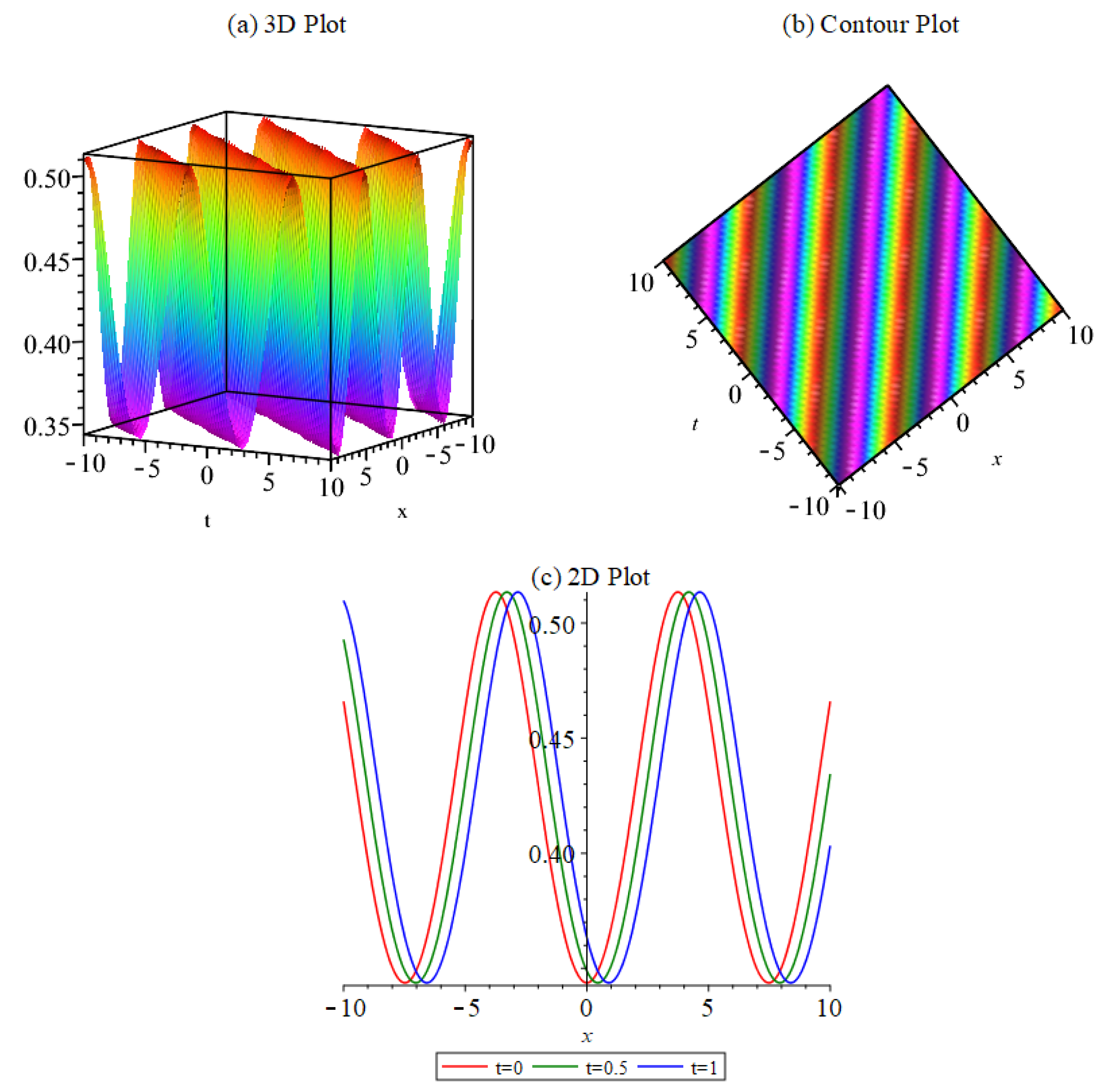
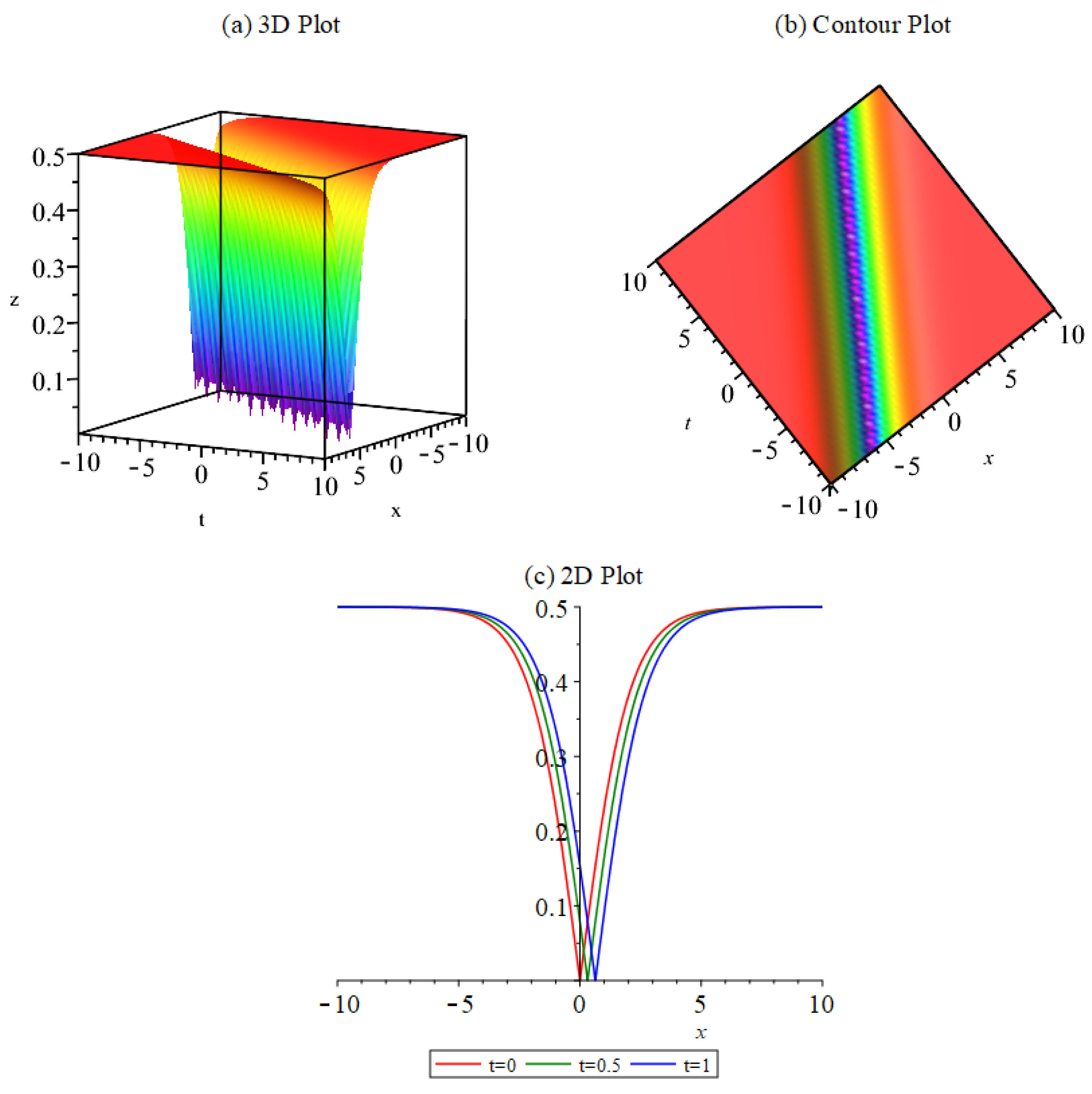
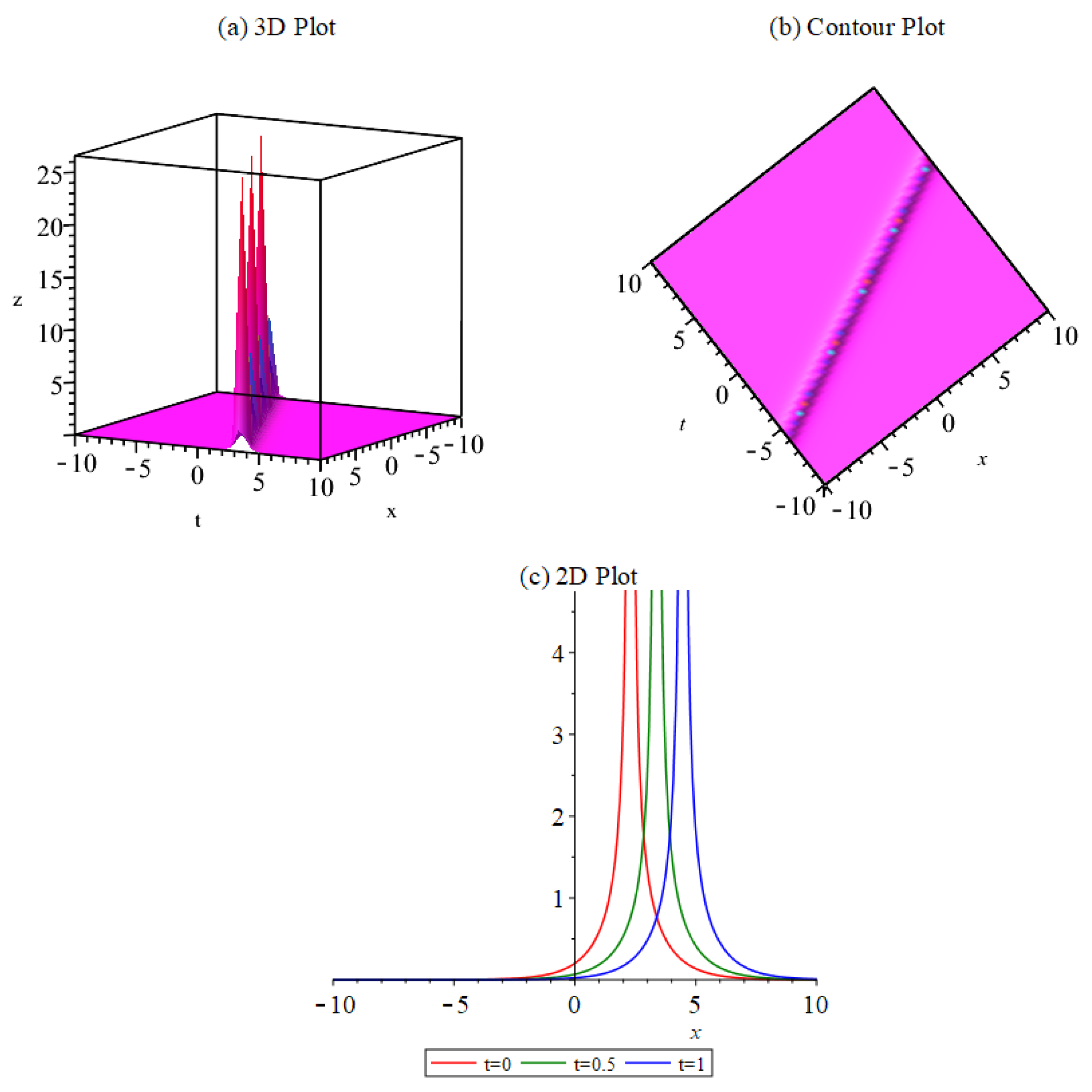
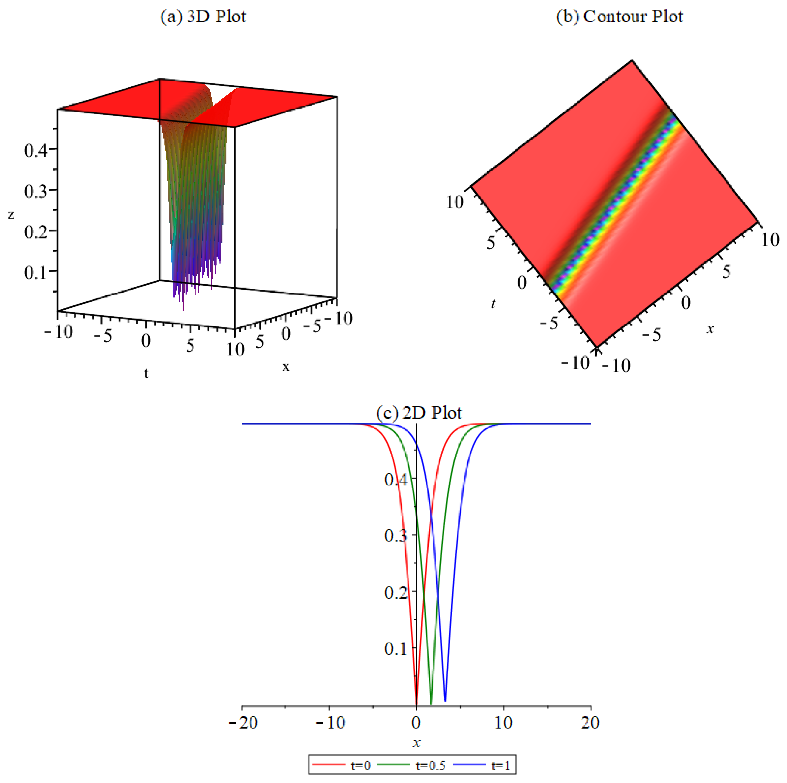
4. The Graphical Representations

In this section, we give the 2D, 3D, and contour plots of some of the results. Plots of the solutions have an important place for understanding the motion of the wave. Firstly, plots were drawn for Equation (21) when $c_1=0.1, c_2=1, \gamma =2.1, \nu =0.9, \Phi =0.6$ as follows (Figure 1):

Then, plots were drawn for Equation (24) when ${\rho }_0=0.2, {\rho }_1=0.8, C=1,\gamma =0.4,$ $\Phi =0.6$ as follows (Figure 2):

Then, plots were drawn for Equation (26) when ${\rho }_1=0.1,C=0.1, \gamma =2, \Phi =0.1$ as follows (Figure 3):

Finally, plots were drawn for Equation (32) when $a=2.7,C_1=1,\gamma =0.1,\Phi =0.8$ as follows (Figure 4):

5. Modulation Instability (MI) Analysis

MI will be investigated in this section and a steady-state solution to Equation (10) is given as follows [34,35,36]:

$$\vartheta (x,t)=\left(\psi \left(x,t\right)+\sqrt{\phi }\right)e^{i\phi x}.$$

(33)

If we are substituting Equation (33) into Equation (10) and linearising the equation, the following ODE is obtained

$$i\left(\gamma {\psi }_{xxx}+{\psi }_t+2\phi {\psi }_x\right)-3\gamma \phi {\psi }_{xx}+{\psi }_{xx}+4\phi \psi +2\phi {\psi }^{*},$$

(34)

where ${\psi }^{*}\left(x,t\right)$ is the conjugate of $\psi \left(x,t\right).$ For solving Equation (34), we suppose the general solutions of the following form:

$$\psi \left(x,t\right)={\alpha }_1{e}^{i\left(\rho x-\nu t\right)}+{\alpha }_2{e}^{-i\left(\rho x-\nu t\right)},$$

(35)

where $\rho$ and $\nu$ denote, respectively, the wave number and the frequency of the perturbations. Putting the supposed solution to Equation (35) into Equation (34), and seperating the coefficients of the $e^{i\left(\rho x-\nu t\right)}$ and $e^{-i\left(\rho x-\nu t\right)},$ the following relation is obtained:

$$-3\phi \gamma {\rho }^2+{\rho }^3\gamma -2\rho \phi +{\rho }^2+\nu =0.$$

(36)

If we solve the dispersion relation as above for $\rho ,$ we get:

$$\begin{array}{cc}\mathsf{\Psi }\left(v\right)=\hfill & \frac{36{\phi }^2{\gamma }^2+6\phi \gamma {\left(216{\phi }^3{\gamma }^3-108{\gamma }^2\nu +12\gamma \sqrt{\mathsf{\Delta }}-8\right)}^{1/3}-2{\left(216{\phi }^3{\gamma }^3-108{\gamma }^2\nu +12\gamma \sqrt{\mathsf{\Delta }}-8\right)}^{1/3}}{6\gamma {\left(216{\phi }^3{\gamma }^3-108{\gamma }^2\nu +12\gamma \sqrt{\mathsf{\Delta }}-8\right)}^{1/3}}\hfill \\ \hfill & \\ \hfill & \frac{+{\left(216{\phi }^3{\gamma }^3-108{\gamma }^2\nu +12\gamma \sqrt{\mathsf{\Delta }}-8\right)}^{1/3}+4}{6\gamma {\left(216{\phi }^3{\gamma }^3-108{\gamma }^2\nu +12\gamma \sqrt{\mathsf{\Delta }}-8\right)}^{1/3}},\hfill \end{array}$$

(37)

where $\mathsf{\Delta }=-108{\phi }^4{\gamma }^2+\left(-324{\gamma }^3\nu -24\gamma \right){\phi }^3-12{\phi }^2+81{\gamma }^2{\nu }^2+12\nu .$

We can say that from the dispersion relation, if

$$-108{\phi }^4{\gamma }^2+\left(-324{\gamma }^3\nu -24\gamma \right){\phi }^3-12{\phi }^2+81{\gamma }^2{\nu }^2+12\nu >0,$$

and

$$6\gamma {\left(216{\phi }^3{\gamma }^3-108{\gamma }^2\nu +12\gamma \sqrt{\mathsf{\Delta }}-8\right)}^{1/3}\ne 0,\mathsf{\Psi }\left(v\right),$$

is real. Then, against small perturbations, the steady state is stable. In contrast, the steady-state solution is always unstable if

$$-108{\phi }^4{\gamma }^2+\left(-324{\gamma }^3\nu -24\gamma \right){\phi }^3-12{\phi }^2+81{\gamma }^2{\nu }^2+12\nu <0,$$

and

$$6\gamma {\left(216{\phi }^3{\gamma }^3-108{\gamma }^2\nu +12\gamma \sqrt{\mathsf{\Delta }}-8\right)}^{1/3}\ne 0.$$

The rate of growth of the MI gives spectrum $G(\Omega )$ as

$$G(\Omega )=2IM\left(\rho \right).$$

The MI gain spectrum for $\phi =9,\gamma =3$ is given by Figure 5 as follows:

6. Conclusions

In our paper, we have successfully derived closed-form traveling wave solutions for complex HDM by using a straightforward approach via the modified simple equation and generalized and modified Kudryashov methods. When we compared our findings to the previous literature, we discovered a diverse range of solutions, each showcasing distinct behaviors. These newly derived solutions are both novel and unique, as they have not been reported before and they hold great promise for addressing real-world challenges related to complex HDM in diverse domains of physics and engineering. In other words, these innovative soliton-type solutions have the potential to make significant contributions to fields like plasma physics, fusion energy research, astrophysics, and space studies. The techniques employed are shown to be robust and highly efficient. Modulation instability (MI) analysis is examined. We also offer visual representations, namely 2D, 3D, and contour plots for the acquired solutions. Graphical representations are valuable for comprehending wave motions.

References

1. Ghanim, F.; Batiha, B.; Ali, A.H.; Darus, M. Geometric Properties of a Linear Complex Operator on a Subclass of Meromorphic Functions: An Analysis of Hurwitz-Lerch-Zeta Functions. Appl. Math. Nonlinear Sci. 2023. [Google Scholar] [CrossRef]
2. Nuaimi, M.A.; Jawad, S. Modelling and stability analysis of the competitional ecological model with harvesting. Commun. Math. Biol. Neurosci. 2022, 2022, 47. [Google Scholar]
3. Yang, X.; Wu, L.; Zhang, H. A space-time spectral order sinc-collocation method for the fourth-order nonlocal heat model arising in viscoelasticity. Appl. Math. Comput. 2023, 457, 128192. [Google Scholar] [CrossRef]
4. Wang, W.; Zhang, H.; Jiang, X.; Yang, X. A high-order and efficient numerical technique for the nonlocal neutron diffusion equation representing neutron transport in a nuclear reactor. Ann. Nucl. 2024, 195, 110163. [Google Scholar] [CrossRef]
5. Zhou, Z.; Zhang, H.; Yang, X. H1-norm error analysis of a robust ADI method on graded mesh for three-dimensional subdiffusion problems. Numer. Algor. 2023, 1–19. [Google Scholar] [CrossRef]
6. Zhang, H.; Yang, X.; Tang, Q.; Xu, D. A robust error analysis of the OSC method for a multi-term fourth-order sub-diffusion equation. Comput. Math. Appl. 2022, 109, 180–190. [Google Scholar] [CrossRef]
7. Srivastava, H.M.; Baleanu, D.; Machado, J.A.T.; Osman, M.S.; Rezazadeh, H.; Arshed, S.; Gunerhan, H. Traveling wave solutions to nonlinear directional couplers by modified Kudryashov method. Phys. Scr. 2020, 95, 075217. [Google Scholar] [CrossRef]
8. Rizvi, S.T.R.; Khan, S.U.D.; Hassan, M.; Fatima, I.; Khan, S.U.D. Stable propagation of optical solitons for nonlinear Schrdinger equation with dispersion and self phase modulation. Math. Comput. Simul. 2021, 179, 126–136. [Google Scholar] [CrossRef]
9. Seadawy, A.; Alamri, S.Z. Mathematical methods via the nonlinear two-dimensional water waves of Olver dynamical equation and its exact solitary wave solutions. Results Phys. 2018, 8, 286–291. [Google Scholar] [CrossRef]
10. Zhang, Z. Jacobi elliptic function expansion method for the mKdVZK and the Hirota equations. Rom. J. Phys. 2015, 60, 1384–1394. [Google Scholar]
11. Raza, N.; Kazmi, S.S. Qualitative analysis and stationary optical patterns of nonlinear Schrödinger equation including nonlinear chromatic dispersion. Opt. Quantum Electron. 2023, 55, 718. [Google Scholar] [CrossRef]
12. Hashemi, M.S.; Mirzazadeh, M. Optical solitons of the perturbed nonlinear Schrdinger equation using Lie symmetry method. Optik 2023, 281, 170816. [Google Scholar] [CrossRef]
13. Gao, W.; Ismael, H.F.; Husien, A.M.; Bulut, H.; Baskonus, H.M. Optical soliton solutions of the cubic-quartic nonlinear Schrödinger and resonant nonlinear Schrödinger equation with the parabolic law. Appl. Sci. 2019, 10, 219. [Google Scholar] [CrossRef]
14. Akbulut, A.; Kaplan, M.; Tascan, F. Conservation laws and exact solutions of Phi-Four (Phi-4) equation via the (G’/G, 1/G)-expansion method. Z. für Naturforschung A 2016, 71, 439–446. [Google Scholar] [CrossRef]
15. Kaplan, M.; Ozer, M.N. Multiple-soliton solutions and analytical solutions to a nonlinear evolution equation. Opt. Quantum Electron. 2018, 50, 2. [Google Scholar] [CrossRef]
16. Zhou, Q.; Kumar, D.; Mirzazadeh, M.; Eslami, M.; Rezazadeh, H. Optical soliton in nonlocal nonlinear medium with cubic-quintic nonlinearities and spatio-temporal dispersion. Acta Phys. Pol. A 2018, 134, 1204–1210. [Google Scholar] [CrossRef]
17. Ma, W.X.; Lee, J.H. A transformed rational function method and exact solutions to the dimensional Jimbo-Miwa equation. Chaos Solitons Fractals 2009, 42, 1356–1363. [Google Scholar] [CrossRef]
18. Hereman, W.; Zhuang, W. Symbolic Computation of Solitons via Hirota’s Bilinear Method; Department of Mathematical and Computer Sciences, Colorado School of Mines: Golden, CO, USA, 1994. [Google Scholar]
19. Alotaibi, M.F.; Raza, N.; Rafiq, M.H.; Soltani, A. New solitary waves, bifurcation and chaotic patterns of Fokas system arising in monomode fiber communication system. Alex. Eng. J. 2023, 67, 583–595. [Google Scholar] [CrossRef]
20. Raza, N.; Seadawy, A.R.; Kaplan, M.; Butt, A.R. Symbolic computation and sensitivity analysis of nonlinear Kudryashov’s dynamical equation with applications. Phys. Scr. 2021, 96, 105216. [Google Scholar] [CrossRef]
21. Raza, N.; Rani, B.; Chahlaoui, Y.; Shah, N.A. A variety of new rogue wave patterns for three couplednonlinear Maccari’s models in complex form. Nonlinear Dyn. 2023, 111, 18419–18437. [Google Scholar] [CrossRef]
22. Zayed, E.M.E.; Ibrahim, S.H. Exact solutions of nonlinear evolution equations in mathematical physics using the modified simple equation method. Chin. Phys. Lett. 2012, 29, 060201. [Google Scholar] [CrossRef]
23. Xia, F.L.; Jarad, F.; Hashemi, M.S.; Riaz, M.B. A reduction technique to solve the generalized nonlinear dispersive mK(m,n) equation with new local derivative. Results Phys. 2022, 38, 105512. [Google Scholar] [CrossRef]
24. Hashemi, M.S.; Malekinagad, J.; Marasi, H.R. Series solution of the system of fuzzy differential equations. Adv. Fuzzy Syst. 2012, 2012, 407647. [Google Scholar] [CrossRef]
25. Sugati, T.G.; Seadawy, A.R.; Alharbey, R.; Albarakati, W. Nonlinear physical complex hirota dynamical system: Construction of chirp free optical dromions and numerical wave solutions. Chaos Solitons Fractals 2022, 156, 111788. [Google Scholar] [CrossRef]
26. Ali, K.K.; Tarla, S.; Ali, M.R.; Yusuf, A.; Yilmazer, R. Consistent solitons in the plasma and optical fiber for complex hirota-dynamical model. Results Phys. 2023, 47, 106393. [Google Scholar] [CrossRef]
27. Seadawy, A.R.; Abdullah, A. Nonlinear complex physical models: Optical soliton solutions of the complex hirota dynamical model. Indian J. Phys. 2021, 95, 489–498. [Google Scholar] [CrossRef]
28. Bekir, A.; Zahran, E. New description for the bright, dark periodic solutions to the complex hirota-dynamical model. Authorea Prepr. 2020. [Google Scholar]
29. Kudryashov, N.A. Solitary and periodic waves of the hierarchy for propagation pulse in optical fiber. Optik 2019, 194, 163060. [Google Scholar] [CrossRef]
30. Kudryashov, N.A. One method for finding exact solutions of nonlinear differential equations. Commun. Nonlinear Sci. Numer. Simul. 2012, 17, 2248–2253. [Google Scholar] [CrossRef]
31. Hosseini, K.; Ansari, R. New exact solutions of nonlinear conformable time-fractional Boussinesq equations using the modified Kudryashov method. Waves Random Complex Media 2017, 27, 628–636. [Google Scholar] [CrossRef]
32. Akbulut, A.; Arnous, A.H.; Hashemi, M.S.; Mirzazadeh, M. Solitary waves for the generalized nonlinear wave equation in (3+1) dimensions with gas bubbles using the Nnucci’s reduction, enhanced and modified Kudryashov algorithms. J. Ocean. Eng. Sci. 2022. [Google Scholar] [CrossRef]
33. Karakoc, S.B.G.; Ali, K.K. Theoretical and computational structures on solitary wave solutions of Benjamin Bona Mahony-Burgers equation. Tbil. Math. J. 2021, 14, 33–50. [Google Scholar] [CrossRef]
34. Ay, N.G.; Yasar, E. Multi wave, kink, breather, interaction solutions and modulation instability to a conformable third order nonlinear Schrödinger equation. Opt. Quantum Electron. 2023, 55, 360. [Google Scholar]
35. Tariq, K.U.; Inc, M.; Kazmi, S.M.R.; Alhefth, R.K. Modulation instability, stability analysis and soliton solutions to the resonance nonlinear Schrödinger model with Kerr law nonlinearity. Opt. Quantum Electron. 2023, 55, 838. [Google Scholar] [CrossRef]
36. Xiang, Y.; Wen, S.; Dai, X.; Tang, Z.; Su, W.; Fan, D. Modulation instability induced by nonlinear dispersion in nonlinear metamaterials. Opt. Soc. Am. 2007, 24, 3058–3063. [Google Scholar] [CrossRef]
Figure 1. 2D and 3D plots of Equation (21).
Mathematics 11 04851 g001
Figure 2. 2D and 3D plots of Equation (24).
Mathematics 11 04851 g002
Figure 3. 2D and 3D plots of Equation (26).
Mathematics 11 04851 g003
Figure 4. 2D and 3D plots of Equation (32).
Mathematics 11 04851 g004
Figure 5. The MI gain spectrum.
Mathematics 11 04851 g005
Disclaimer/Publisher’s Note: The statements, opinions and data contained in all publications are solely those of the individual author(s) and contributor(s) and not of MDPI and/or the editor(s). MDPI and/or the editor(s) disclaim responsibility for any injury to people or property resulting from any ideas, methods, instructions or products referred to in the content.