Article

New (3+1)-Dimensional Kadomtsev–Petviashvili–Sawada– Kotera–Ramani Equation: Multiple-Soliton and Lump Solutions

by
Abdul-Majid Wazwaz
1,†,
Ma’mon Abu Hammad
2,
Ali O. Al-Ghamdi
3,
Mansoor H. Alshehri
4 and
Samir A. El-Tantawy
5,*
1
Department of Mathematics, Saint Xavier University, Chicago, IL 60655, USA
2
Department of Mathematics, Al-Zaytoonah University of Jordan, Amman 11733, Jordan
3
Biology Department, Faculty of Science and Arts, Al-Mikhwah, Al-Baha University, Al-Baha 1988, Saudi Arabia
4
Department of Mathematics, College of Science, King Saud University, P.O. Box 2455, Riyadh 11451, Saudi Arabia
5
Department of Physics, Faculty of Science, Port Said University, Port Said 42521, Egypt
*
Author to whom correspondence should be addressed.
This legendary researcher is the leader of the group and has done most of this work.
Mathematics 2023, 11(15), 3395; https://doi.org/10.3390/math11153395
Submission received: 18 May 2023 / Revised: 20 June 2023 / Accepted: 1 August 2023 / Published: 3 August 2023
(This article belongs to the Special Issue Exact Solutions and Numerical Solutions of Differential Equations)

Abstract

:
In this investigation, a novel (3+1)-dimensional Lax integrable Kadomtsev–Petviashvili–Sawada–Kotera–Ramani equation is constructed and analyzed analytically. The Painlevé integrability for the mentioned model is examined. The bilinear form is applied for investigating multiple-soliton solutions. Moreover, we employ the positive quadratic function method to create a class of lump solutions using distinct parameters values. The current study serves as a guide to explain many nonlinear phenomena that arise in numerous scientific domains, such as fluid mechanics; physics of plasmas, oceans, and seas; and so on.

1. Introduction

Over the previous few decades, studying higher-dimensional integrable differential equations has gained immense research interest due to its significance in solitary wave theory [1,2]. These equations have exerted considerable effects supporting the developments of scientific areas. Nonlinear integrable models appear in many scientific disciplines, such as mathematical physics, plasma physics, fluid mechanics, nonlinear optics, ocean waves, tsunamis, fluid dynamics, electrical engineering, atmospheric science, matter-wave pulses in Bose–Einstein condensates, and solitary wave (SW) theory [3,4,5,6,7,8,9,10]. A nonlinear system becomes integrable if it belongs to one of the integrable senses, namely the Liouville integrable sense, Painlevé integrable sense, Lax integrable sense, infinite symmetry integrable sense, etc. It is known that the idea of integrability has no one definition; in discussing the integrability of any system, it is necessary to specify the integrability sense of the examined system [11,12,13,14,15,16,17,18,19]. The mathematical or physical properties of higher-dimensional integrable models have attracted a considerable number of research investigations. This is due to the fact that the integrability phenomenon is an essential characteristic that led to several scientific applications [20,21,22,23,24,25,26,27].
This has led to investing a significant amount of research being conducted to explicitly introduce extensions to integrable hierarchies. Thus, this led to the introduction of some extensions of known integrable models. We can study several important results in SW theory thanks to the integrable extensions of the well-known models in higher dimensions [27,28,29]. Due to the existence of the Lax pair or Painlevé property, the integrable models become completely solvable. The combinations of two or more components of an integrable hierarchy have recently attracted some useful works that led to new integrable systems with reliable results.
Lately, various theoretical proposals to form linear structures or combinations of two or more arbitrary integrable members of a specific hierarchy have been introduced [3,4,5,6,7,8,9,10,11,12,13,14]. For example, the Burgers equation was combined with the STO equation to form an integrable linear system that led to kink solutions and molecule solutions [5,6,7]. Other works of combining the standard KdV equation with any of the fifth-order KdV equations were given in [3,4,5,6,7,8,9,10] and some of the references therein. In [3], a linear combination of the standard KdV equation and the fifth–order Sawada–Kotera equation, a member of the KdV hierarchy [3,4,5], was proposed as
u t + a ( 3 u 2 + u x x ) x + b ( 15 u 3 + 15 u u x x + u x x x x ) x = 0 ,
called the KdV–SK–R equation. Hirota and Ito [4] utilized this equation to explain the resonances of solitons in a one-dimensional space. In Equation (1), for b = 0 , the KdV equation is recovered. However, for a = 0 , the fifth-order Sawada–Kotera equation is recovered.
Using the same sense of the KdV–SK–R Equation (1), the authors in Ref. [4] developed a new Lax integrable equation given as
u x t + ( 3 u 2 + u x x ) x x + ( 15 u 3 + 15 u u x x + u x x x x ) x x + σ u y y = 0 ,
which will be called Kadomtsev–Petviashvili–Sawada–Kotera–Ramani (KP–SK–R) equation. Also, this equation can be reduced to Equation (1) for σ = 0 . Also, in Ref. [4], the Lax pair was constructed to confirm its Lax integrability; by introducing the potential function, an infinite number of conservation laws are introduced. Additionally, this equation was applied to characterize the solitons’ resonances in a two-dimensional space. Motivated by the above scientific applications and many other, the aim of this paper is to present a study on integrability of a (3+1)-dimensional extension of the KP–SK–R Equation (2) that takes the sixth-order form
u x t + a ( 3 u 2 + u x x ) x x + ( 15 u 3 + 15 u u x x + u x x x x ) x x + α 1 u y y + α 2 u z z + β 1 u x y + β 2 u y z + β 3 u x z = 0 .
The nonlinear integrable equations have been thoroughly investigated aiming to achieve more new results. Researchers were interested to derive many scientific solutions, such as multiple-soliton solutions, breather solutions, kink solutions, lump solutions, rogue wave (RW) solutions, and many others. Numerous helpful discoveries were made that aided in the investigation of certain fresh physical characteristics of various applications. The essential characteristics of lump solutions (LSs), which are sometimes called rational function (RF) solutions, in physics and many other nonlinear disciplines have attracted the attention of several scholars in recent years. Lumps differ from solitons because of their locality with higher amplitude and rapididity [3,4,5,6,7,8,9,10,11,12,13,14,15,16,17,18,19]. The lump solution (LS), a form of RF solution, has received a lot of interest in the domains of mathematical physics and science [3,4,5,6,7,8,9,10,11,12,13,14,15,16]. Lumps are a type of RF solution and are localized in all space directions, whereas solitons are exponentially localized in particular directions [3,4,5,6,7,8,9,10,11,12,13,14,15,16]. However, rogue waves (RWs) are localized in both space-time, emerge out of nowhere, and vanish without leaving any trace. Lump waves appear in many nonlinear systems, such as oceanography, shallow water waves, nonlinear optical fibers, and biophysics. Studying the extended integrable equations significantly improves SW theory and sheds more light on the physical significance of the obtained solutions. To find multiple-soliton solutions and LSs, the Hirota bilinear form is an effective technique to achieve this purpose.
The SW solutions for several nonlinear models have been obtained using some effective analytical techniques, including the inverse scattering method, the Hirota method, Darboux transformation technique, and Painlevé expansion method. One of the best methods for creating soliton solutions using the dependent variable transformation and conventional parameter stretching is Hirota’s bilinear method.
In this article, we will first demonstrate that the new constructed (3+1)-dimensional Lax integrable KP–SK–R model (3) fails the complete Painlevé integrability. After that we will derive multiple-soliton solutions that play an important role in revealing qualitative and quantitative features of nonlinear scientific via using the simplified Hirota’s scheme [3,4,5,6,7,8,9,10,11,12]. Additionally, a class of LSs for this novel equation can be established using various values of the utilized parameters.

2. Formulation of a New (3+1)-Dimensional KP–SK–R Equation

Based on the literature works, the following new extended KP–SK–R equation is constructed
u x t + ( 3 u 2 + u x x ) x x + ( 15 u 3 + 15 u u x x + u x x x x ) x x + α 1 u y y + α 2 u z z + β 1 u x y + β 2 u y z + β 3 u x z = 0 ,
where α i , i = 1 , 2 , and β j ; j = 1 , 2 , 3 are non-zero arbitrary parameters; and u u ( x , y , z , t ) . Moreover, the extended KP–SK–R Equation (4) includes four additional terms, namely α 2 u z z , β 1 u x y , β 2 u y z , and β 3 u x z when compared with Equation (2). Following [4], the newly extended Equation (4) is Lax integrable.

3. Painlevé Analysis to a Related Equation

Numerous important characteristics, including the Hamiltonian structure, the Lax pair, an infinite number of conservation laws, and an infinite number of symmetries, can describe the integrability of different nonlinear evolution equations. In this investigation, we aim to study the Painlevé integrability of Equation (4). To do this, we adhere to the Painlevé analysis described in Refs. [3,4,5,6,7,8,9,10] and some references therein.

Painlevé Analysis

Painlevé integrability of nonlinear PDEs can be examined using Painlevé analysis. It is important to know that the meaning of Painlevé integrability of nonlinear PDEs is that the solution is single-valued in the vicinity of a movable singularity manifold. Weiss, Tabor, and Carnevale (WTC) [7] developed an algorithm ( WTC method) to study the compatibility criteria for Painlevé integrability.
It is assumed that the solution to Equation (4) is a Laurent expansion about a singular manifold ψ ψ ( x , y , z , t ) as
u = k = 0 u k ψ k γ .
For applying the Painlevé test, you must first (i) compute the leading order and coefficients, (ii) identify the resonant points, and then (iii) check the compatibility conditions. We shall investigate each idea in the sections that follow [6,7,8,9,10,11,12,13,14,15,16,17,18,19].
(i) 
Leading order behavior and coefficients:
To obtain the leading order behavior and coefficients, the following ansatz is considered
u = u 0 ϕ α ,
in Equation (4) to obtain the following two distinct cases:
( i ) α = 2 , u 0 = 2 ϕ x , ( i i ) α = 2 , u 0 = 4 ϕ x .
(ii) 
Resonant points:
Our goal is to identify the resonant points, or the values of j at which arbitrary functions can be introduced into the Laurent series
u = j = 0 u j ϕ j + k ,
and it is single-valued, close to the singularity manifold ϕ . To accomplish this goal, we use
u = u 0 ϕ 1 + u j ϕ j 1 ,
in Equation (4), following the WTC analysis [5], and balancing the most dominant terms, we finally obtain:
(i)
The principal branch: k = 1 , 2 , 3 , 6 , 7 , 10 ;
(ii)
The secondary branch: k = 2 , 1 , 5 , 6 , 7 , 12 .
where each branch includes six resonance points due to the sixth-order of the linear structure of Equation (4).
(iii) 
Verifying compatibility conditions
We refer to the works in Refs. [3,4,5,6,7,8,9,10,11,12,13,14,15,16] to confirm the compatibility conditions. The resonance at k = 1 relates to the arbitrariness of singular manifold ψ = 0 for the principal branch (i). Moreover, the Painlevé compatibility, while working for levels 2 , 3 , 6 , and 7, fails at level 10.
For the secondary branch, the Painlevé compatibility, while working for levels 6 and 7, fails for levels 5 and 12. Based on this, we conclude that the KP–SK–R (4) does not pass the Painlevé test, and presumably, it is not Painlevé integrable.
As stated earlier, the newly extended Equation (4) is Lax integrable as confirmed in Ref. [4]. Using the results in [3,4,5,6,7], we will pursue our work to determine multiple-soliton solutions and a variety of LSs.

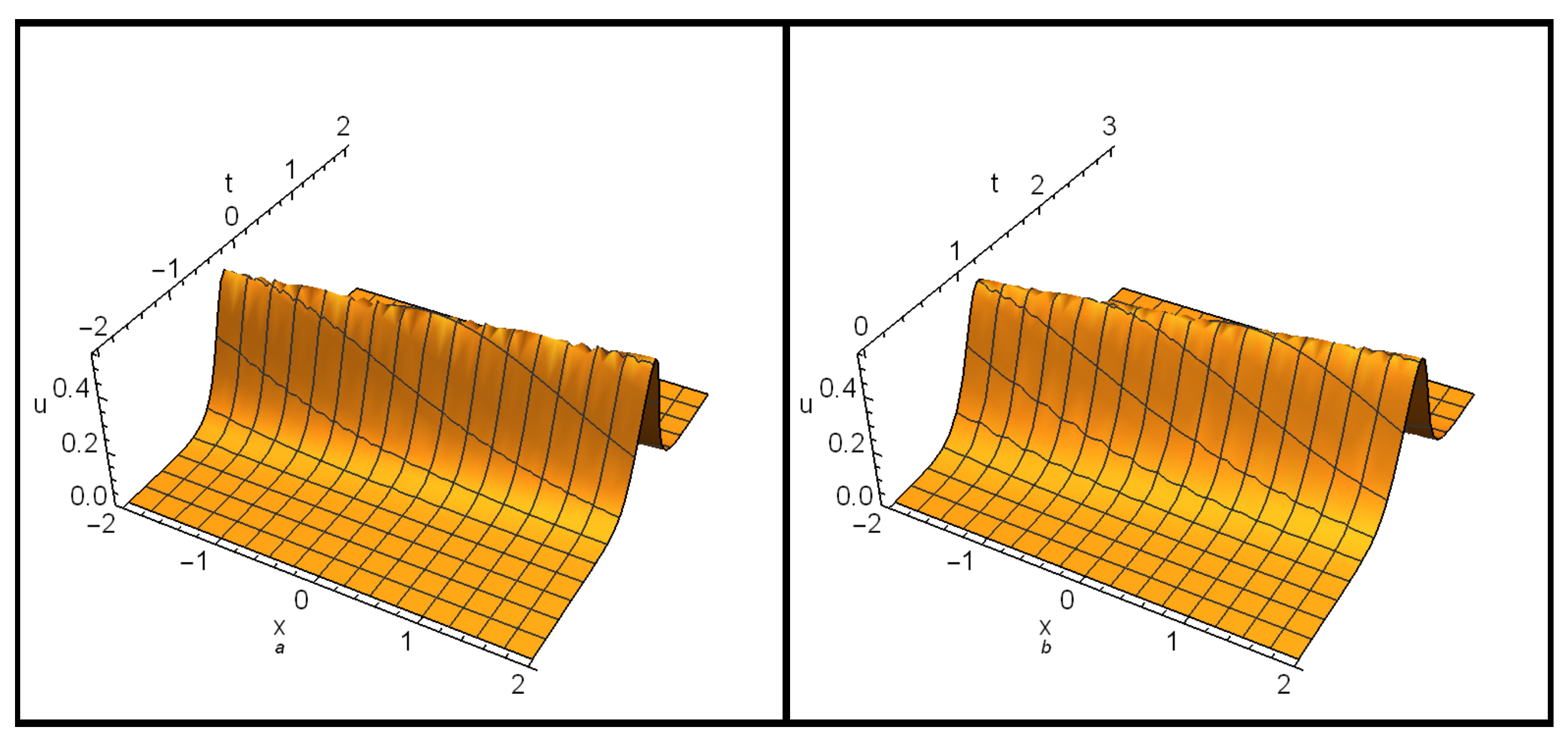
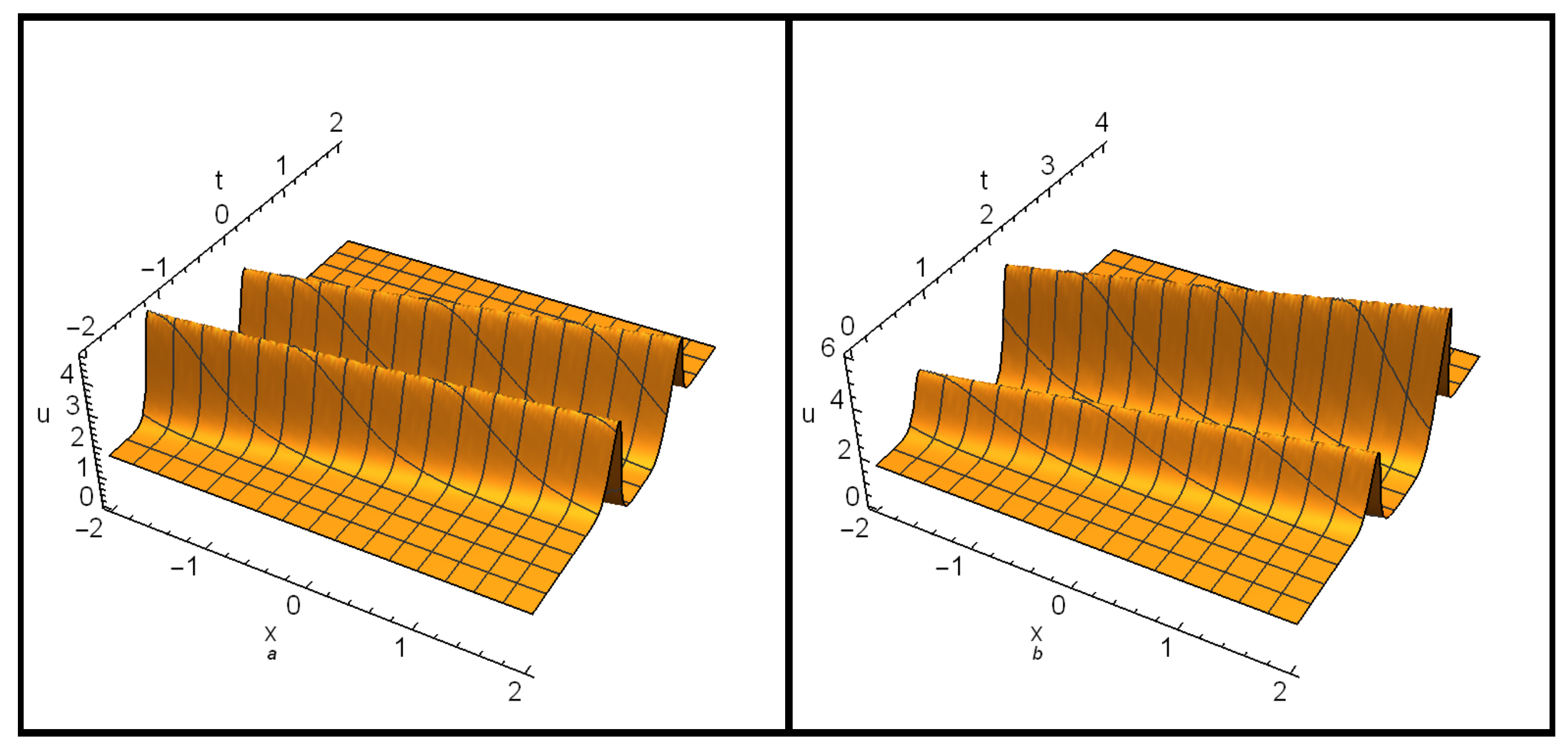
4. Multiple-Soliton Solutions

Here, we plan to obtain the dispersion relation (DR) and multiple-soliton solutions for the KP–SK–R Equation (4) and hence obtain the phase shifts (Phs) of the soliton interaction. To achieve that, we insert the following solution into the linear parts of Equation (4)
u i = e θ i ,
in order to obtain the following DR:
c i = k i 6 + k i 4 + α 1 r i 2 + α 2 s i 2 + β 1 k i r i + β 2 r i s i + β 3 k i s i k i ,
with phase variables θ i = R i c i t where R i = k i x + r i y + s i z , where i = 1 , 2 , , N . Accordingly, we obtain
θ i = k i x + r i y + s i z k i 6 + k i 4 + α 1 r i 2 + α 2 s i 2 + β 1 k i r i + β 2 r i s i + β 3 k i s i k i t ,
where i = 1 , 2 , , N . Using the following transformation:
u i = 2 ( ln f i ) x x ,
in Equation (4) to obtain multiple-soliton solutions. Here, f i f i ( x , y , z , t ) gives the auxiliary function, where i = 1 , 2 , 3 , corresponding to, one-, two, three-solitons and so on.
Now, to obtain the one-soliton solution, the following value is considered
f 1 = 1 + e θ 1 ,
where θ 1 can be obtained from Equation (12) for i = 1 . Accordingly, the following one-soliton solution is obtained
u 1 = 2 k 1 2 e k 1 x + r 1 y + s 1 z k 1 6 + k 1 4 + α 1 r 1 2 + α 2 s 1 2 + β 1 k 1 r 1 + β 2 r 1 s 1 + β 3 k 1 s 1 k 1 t ( 1 + e θ 1 ) 2 .
The profile of one-soliton solution (15) is illustrated in Figure 1 for ( k 1 , r 1 , s 1 ) = ( 1 , 1 , 1 ) and ( α 1 , α 2 , β 1 , β 3 , β 3 ) = ( 2 , 2 , 0.1 , 0.1 , 0.1 ) . Here, Figure 1a for ( y , z ) = ( 0 , 0 ) and Figure 1b for ( y , z ) = ( 5 , 5 ) .
To obtain two-soliton solutions, the following function f 2 is introduced
f 2 = f 1 + e θ 2 + a 12 e θ 1 + θ 2 ,
where a 12 denotes the Phs. To estimate the value of a 12 , we insert Equation (16) into Equation (4) to obtain
a 12 = k 1 2 k 2 2 ( k 1 k 2 ) 2 ( 5 k 1 2 5 k 1 k 2 + 5 k 2 2 + 3 ) + α 1 ( k 1 r 2 k 2 r 1 ) 2 + α 2 ( k 1 s 2 k 2 s 1 ) 2 + β 2 ( k 1 s 2 k 2 s 1 ) ( k 1 r 2 k 2 r 1 ) k 1 2 k 2 2 ( k 1 + k 2 ) 2 ( 5 k 1 2 + 5 k 1 k 2 + 5 k 2 2 + 3 ) + α 1 ( k 1 r 2 k 2 r 1 ) 2 + α 2 ( k 1 s 2 k 2 s 1 ) 2 + β 2 ( k 1 s 2 k 2 s 1 ) ( k 1 r 2 k 2 r 1 ) ,
which can be generalized as
a i j = k i 2 k j 2 ( k i k j ) 2 ( 5 k i 2 5 k i k j + 5 k j 2 + 3 ) + α 1 ( k i r j k j r i ) 2 + α 2 ( k i s j k j s i ) 2 + β 2 ( k i s j k j s 1 ) ( k i r j k j r i ) k i 2 k j 2 ( k i + k j ) 2 ( 5 k i 2 + 5 k i k j + 5 k j 2 + 3 ) + α 1 ( k i r j k j r i ) 2 + α 2 ( k i s j k j s i ) 2 + β 2 ( k i s j k j s i ) ( k i r j k j r i ) ,
where 1 i < j 3 .
It is clear that the Phs (18) depends on the parameters α 1 , α 2 , β 2 , k n , r n , and s n , n = 1 , 2 , 3 but does not depend on β 1 and β 3 . By inserting Equations (17) and (16) into Equation (13), we obtain the two-soliton solutions.
The profile of the two-soliton solution according to Equations (13) and (16) is illustrated in Figure 2 for ( k 1 , r 1 , s 1 ) = ( 1 , 1 , 1 ) , ( k 2 , r 2 , s 2 ) = ( 0.4 , 0.4 , 0.4 ) , and ( α 1 , α 2 , β 1 , β 3 , β 3 ) = ( 2 , 2 , 0.1 , 0.1 , 0.1 ) . Here, Figure 2a for ( y , z ) = ( 0 , 0 ) and Figure 2b for ( y , z ) = ( 5 , 5 ) .
To obtain the three-soliton solutions, the following value to f 3
f 3 = f 2 + e θ 3 + a 13 e θ 1 + θ 3 + a 23 e θ 2 + θ 3 + a 12 a 23 a 13 e θ 1 + θ 2 + θ 3 .
By inserting Equation (19) into Equation (13), we obtain the three-soliton solutions. Remember that we can obtain N-soliton solutions for finite N, where N 1 .

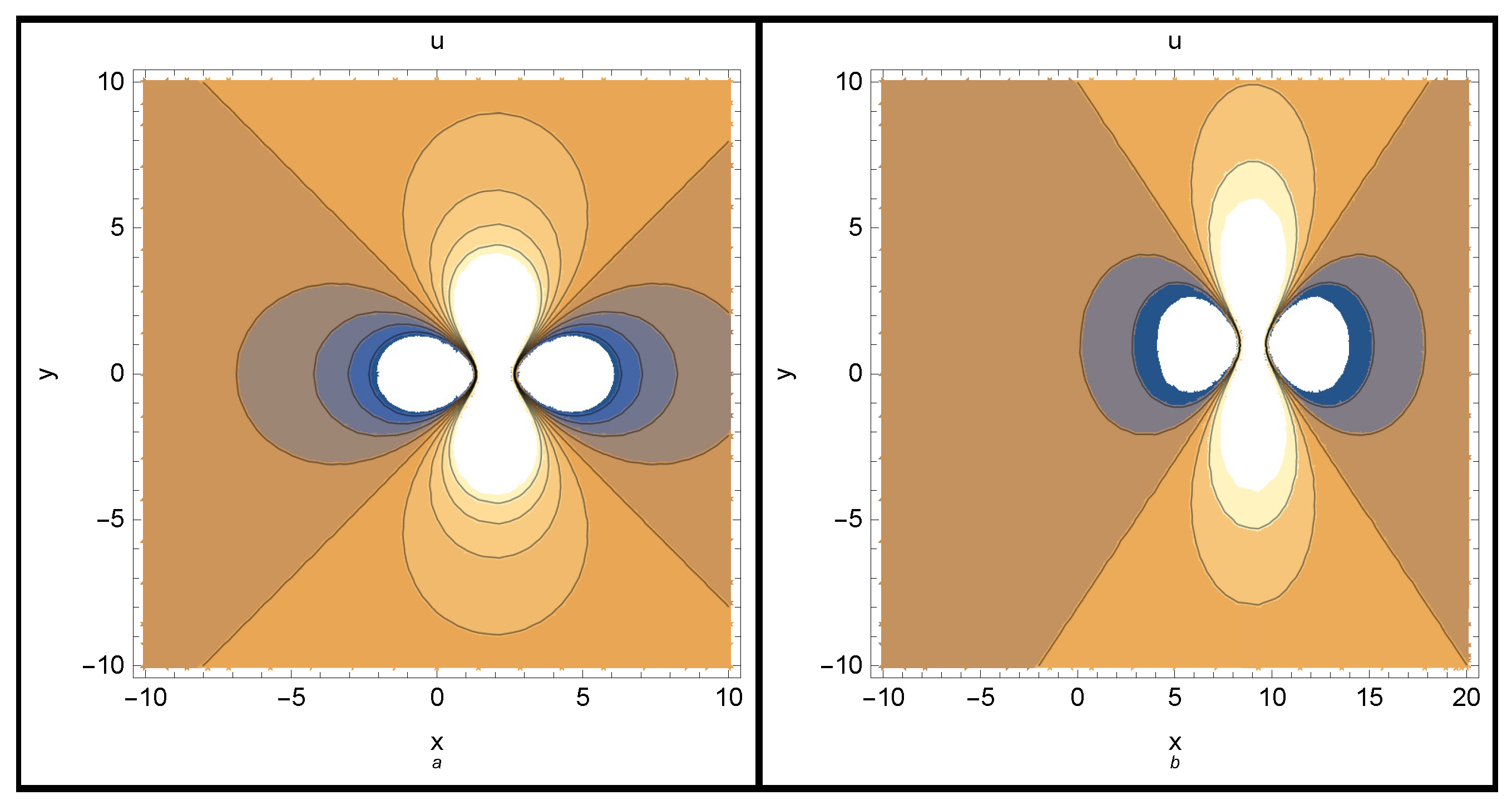
5. Lump Solutions (LSs)

When surface tension dominates the shallow water surface, as in plasma and optical media, LSs are typically created. The generalized positive quadratic function can be used as the foundation for a symbolic computation method to analyze LSs. Here, for deriving a class of LSs for arbitrary values of the parameters, we firstly transform Equation (4) to the bilinear equation in operators form
D x D t + D x 6 + D x 4 + α 1 D y 2 + α 2 D z 2 + | β 1 D x D y + β 2 D y D z + β 3 D x D z f · f = 0 .
Here, D t , D x , D y , and D z represent the Hirota’s bilinear derivative operators. To simplify computational tasks, we consider α 1 = α = 1 , β 1 = β 2 = β 3 = 1 . Accordingly, Equation (20) transforms to
( f f x t f x f t ) + ( f f x x x x x x 6 f x f x x x x x + 15 f x x x x f x x 10 ( f x x x ) 2 ) + ( f f x x x x 4 f x x x f x + 3 ( f x x ) 2 ) ( f f y y ( f y ) 2 ) + ( f f y y f y f y ) + ( f f z z f z f z ) + ( f f x y f x f y ) + ( f f y z f y f z ) + ( f f x z f x f z ) = 0 ,
obtained upon using
u = 2 ( ln f ) x x .
The following presumptions are made in order to obtain the quadratic soliton solutions for Equation (4)
G = A x + B y + C z + D t + E , f = g 2 + h 2 + a 11 .
where G = [ g , h ] T and the coefficients A = [ a 1 , a 6 ] T , B = [ a 2 , a 7 ] T , C = [ a 3 , a 8 ] T , D = [ a 4 , a 9 ] T , E = [ a 5 , a 1 0 ] T , and " T " represents the matrix transpose. Here, a j , 1 j 11 are undermined real parameters. Plugging Equation (23) into Equation (21), we obtain a polynomial in ( x , y , z , t ) variables. To obtain the values of a j , we construct a system with the coefficients of x , y , z , t , x t , y t , z t , x z , x y , y z , x 2 , y 2 , z 2 , t 2 , and the constant terms. The following particular sets of restricting equations on the different parameters are generated by solving the resulting system using Maple; other sets may also be derived.
Case 1.
Using a new set of parameters, we may determine another LS and find
a i = a i & i = 1 , 2 , 3 , 5 , 6 , 8 , a 4 = a 1 ( a 1 2 + a 6 2 ) ( a 2 + a 3 ) a 2 ( a 1 2 + a 6 2 ) ( a 2 a 3 ) a 1 2 ( a 3 2 a 8 2 ) 2 a 1 a 3 a 6 a 8 a 1 ( a 1 2 + a 6 2 ) , a 1 0 , a 7 = a 2 a 6 a 1 , a 1 0 , a 9 = a 1 3 * a 2 ( a 6 + a 8 ) a 1 2 a 6 ( a 2 2 ] a 3 2 ) + a 1 2 * a 6 a 8 ( a 6 a 8 ) + a 6 3 a 2 ( a 1 a 2 ) + a 1 3 a 8 ( a 1 2 a 3 ) + a 1 a 2 a 6 2 a 8 a 1 2 ( a 1 2 + a 6 2 ) , a 1 0 , a 10 = a 5 a 6 a 1 , a 7 = a 1 2 + a 6 a 8 + a 1 4 6 a 1 2 a 6 a 8 4 a 1 2 a 6 a 9 3 a 6 2 a 8 2 2 a 6 , a 11 = 3 ( a 1 2 + a 6 2 ) 3 ( a 1 a 8 a 3 a 6 ) 2 ,
where a 11 > 0 , which must fulfill the following determinant condition
Δ = a 1 a 3 a 6 a 8 0 ,
to ensure a well-defined function f, its positivity, and the localization of u in all space directions, respectively. By substituting Equation (24) into Equation (23), the resulting parameters (24) will generate a class of positive quadratic function (PQF) solutions. According to these values and by using u = 2 ( l n f ) x x , then Equation (4) will yield a first class of LSs as shown below.
For example, by selecting
a i = i & i = 1 , 2 , 3 , 5 , 6 , 8 ,
and using (24), we obtain
a 4 = 1 2 , a 7 = 2 , a 9 = 1 2 , a 10 = 1 , a 11 = 24 ,
which will give the LS
u = S 1 S 2 ,
with
S 1 = 16 t 2 + ( 64 x + 128 y + 96 z + 64 ) t 64 x 2 + ( 256 y 192 z 128 ) x 256 y 2 + ( 384 z 256 ) y 128 z 2 192 z + 704 , S 2 = ( t 2 + ( 4 x 8 y 6 z 4 ) t + 4 x 2 + ( 16 y + 12 z + 8 ) x + 16 y 2 + ( 24 z + 16 ) y + 10 z 2 + 12 z + 52 ) 2 .
Keep in mind that the derived LSs u 0 if and only if g 2 + h 2 .
Case 2.
In this case, we use
a i = a i & i = 1 , 3 , 6 , 7 , 8 , 10 , a 2 = a 1 a 7 a 6 , a 6 0 , a 4 = a 1 2 ( a 6 + a 7 ) ( a 1 a 7 + a 3 a 6 ) + a 1 a 6 2 a 7 ( a 6 + a 7 ) + a 6 2 a 8 ( a 1 a 8 2 a 3 a 6 ) + a 3 a 6 3 ( a 6 + a 7 ) a 1 a 3 2 a 6 2 a 6 2 ( a 1 2 + a 6 2 ) , a 5 = a 1 a 10 a 6 , a 9 = a 1 2 ( a 7 + a 8 ) ( a 6 + a 7 ) + a 6 2 ( a 3 2 + a 7 2 ) + a 6 3 ( a 7 + a 8 ) + a 6 2 a 8 ( a 7 a 8 ) + 2 a 1 a 3 a 6 a 8 a 6 2 ( a 1 2 + a 6 2 ) , a 11 = 3 ( a 1 2 + a 6 2 ) 3 ( a 1 a 8 a 3 a 6 ) 2 , a 11 > 0 ,
which must fulfill the following condition
Δ = a 1 a 2 a 6 a 7 0 ,
to ensure a well-defined function f, its positivity, and the localization of u in all space directions, respectively. By substituting Equation (29) into Equation (23), the resulting parameters (29) will generate a class of PQF solutions. According to these values and by using u = 2 ( l n f ) x x , then Equation (4) will yield a first class of LSs as shown below.
u = 4 ( a 1 2 + a 6 2 ) f 8 ( a 1 g + a 6 h ) 2 f 2 ,
where f , g , and h are defined in Equation (23). Keep in mind that the derived LSs u 0 if and only if g 2 + h 2 .
Case 3.
We use a fresh set of parameters to find another LS, which we have as
a i = a i & i = 1 , 6 , 8 , 9 , 10 , a 2 = a 1 2 + a 6 a 8 + a 1 4 6 a 1 2 a 6 a 8 4 a 1 2 a 6 a 9 3 a 6 2 a 8 2 2 a 1 , a 1 0 , a 3 = a 6 a 8 a 1 , a 4 = ( a 1 2 + a 6 2 ) a 1 4 6 ( a 8 + 2 3 a 9 ) a 6 a 1 2 3 a 6 2 a 8 2 a 1 4 a 6 ( a 6 3 a 8 2 a 9 ) a 1 2 + 3 a 6 3 a 8 2 a 1 a 6 2 , a 6 0 , a 5 = a 1 a 10 a 6 , a 7 = a 1 2 + a 6 a 8 + a 1 4 6 a 1 2 a 6 a 8 4 a 1 2 a 6 a 9 3 a 6 2 a 8 2 2 a 6 , a 11 = 6 a 6 2 ( a 1 2 + a 6 2 ) a 1 2 + 3 a 6 a 8 + a 6 a 9 + a 1 4 6 a 1 2 a 6 a 8 4 a 1 2 a 6 a 9 3 a 6 2 a 8 2 ,
where a 11 > 0 upon proper selections of the parameters, which needs to satisfy the determinant condition. Following the same methodology that was used in the upper part, and by using u = 2 ( l n f ) x x , then Equation (4) will yield a first class of LSs as shown below
For example, by selecting
a 1 = 1 , a 6 = 1 , a 8 = 2 , a 9 = 6 , a 10 = 2 ,
and using (32), we obtain
a 2 = 2 , a 2 = 2 , a 4 = 8 , a 5 = 2 , a 7 = 1 , a 11 = 6 7 ,
which will give the LS
u = W 1 W 2 ,
with
W 1 = 9408 t 2 + ( 2744 x + 392 y 784 z 5488 ) t 196 x 2 + 196 y 2 784 y z + 784 z 2 + 784 x 700 , W 2 = ( 350 t 2 98 t x + 14 t y 28 t z + 7 x 2 + 7 y 2 28 y z + 28 z 2 + 196 t 28 x + 31 ) 2 .
The profile of lump solution (35) is illustrated in Figure 3a and Figure 3b for ( t , z ) = ( 0 , 0 ) and ( t , z ) = ( 1 , 1 ) , respectively.

6. Conclusions

This work aims to explore novel multiple-soliton solutions as well as lump solutions by first developing a new (3+1)-dimensional KP-SK-R equation to portray more dispersion effects in nonlinear science. The newly developed model is obtained by adding four more linear terms to the model proposed in [2]. The Painlevé analysis technique was utilized to prove that this new model fails the Painlevé integrability, but it is Lax integrable, as confirmed in Ref. [2]. In order to display various soliton solutions for the evaluation of phase shifts and dispersion relations, the Hirota approach was used. Using Hirota’s bilinear operator with the help of Maple software, we obtained a class of lump solutions for the bilinear form of the proposed model. Other cases of lump solutions can be provided in a similar fashion. This confirms the criteria that integrability falls in distinct senses such as Liouville integrable sense, Painlevé integrable sense, Lax integrable sense, and infinite symmetry integrable sense. In recent years, fractional calculus has played an important role in a deep understanding of many natural phenomena [30,31,32,33]. Therefore, many methods in the literature used in analyzing fractional differential equations can be applied to analyze the current model in its fractional form.

Author Contributions

Conceptualization, M.A.H. and M.H.A.; Methodology, A.-M.W. and S.A.E.-T.; Software, A.-M.W.; Validation, A.-M.W., M.A.H., A.O.A.-G.and S.A.E.-T.; Formal analysis, A.-M.W., M.A.H., A.O.A.-G.and S.A.E.-T.; Investigation, A.-M.W., Ali O. Al-Ghamdi, M.H.A. and S.A.E.-T.; Resources, A.-M.W.; Writing—original draft, A.-M.W. and S.A.E.-T.; Writing—review & editing, M.H.A. and S.A.E.-T.; Visualization, M.H.A. and S.A.E.-T.; Supervision, A.-M.W.. All authors have read and agreed to the published version of the manuscript.

Funding

This project was supported by Researchers Supporting Project number (RSP2023R411), King Saud University, Riyadh, Saudi Arabia.

Data Availability Statement

Data sharing does not apply to this article as no data sets were generated or analyzed during the current study.

Conflicts of Interest

The authors declare no conflict of interest.

References

  1. Akinyemi, L.; Senol, M.; Az-Zo’Bi, E.; Veeresha, P.; Akpan, U. Novel soliton solutions of four sets of generalized (2+1)-dimensional Boussinesq-Kadomtsev-Petviashvili-like equations. Modern Phys. Lett. B 2022, 36, 2150530. [Google Scholar] [CrossRef]
  2. Tao, G.; Sabi’u, J.; Nestor, S.; El-Shiekh, R.M.; Akinyemi, L.; Az-Zo’bi, E.; Betchewe, G. Dynamics of a new class of solitary wave structures in telecommunications systems via a (2+1)-dimensional nonlinear transmission line. Modern Phys. Lett. B 2022, 36, 2150596. [Google Scholar] [CrossRef]
  3. Ma, P.-L.; Tian, S.-F.; Zhang, T.-T.; Zhang, X.-Y. On Lie symmetries, exact solutions and integrability to the KdV–Sawada–Kotera–Ramani equation. Eur. Phys. J. Plus 2016, 131, 98. [Google Scholar] [CrossRef]
  4. Guo, B. Lax integrability and soliton solutions of the (2+1)–dimensional Kadomtsev–Petviashvili–Sawada–Kotera–Ramani equation. Front. Phys. 2022, 10, 1067405. [Google Scholar] [CrossRef]
  5. Ramani, A. Inverse scattering, ordinary differential equations of Painlevé type and Hirotas bilinear formalism. Ann. N. Y. Acad. Sci. 1981, 373, 54–67. [Google Scholar] [CrossRef]
  6. Hirota, R.; Ito, M. Resonance of solitons in one dimension. J. Phys. Soc. Japan 1983, 52, 744–748. [Google Scholar] [CrossRef]
  7. Weiss, J.; Tabor, M.; Carnevale, G. The Painlevé property of partial differential equations. J. Math. Phys. A 1983, 24, 522–526. [Google Scholar] [CrossRef]
  8. Wazwaz, A.M. N-soliton solutions for the combined KdV-CDG equation and the KdVLax equation. Appl. Math. Comput. 2008, 203, 402–407. [Google Scholar]
  9. Ma, Y.-L.; Wazwaz, A.M.; Li, B.-Q. New extended Kadomtsev-Petviashvili equation: Multiple-soliton solutions, breather, lump and interaction solutions. Nonlinear Dyn. 2021, 104, 1581–1594. [Google Scholar] [CrossRef]
  10. Ma, Y.-L.; Wazwaz, A.M.; Li, B.-Q. Novel bifurcation solitons for an extended Kadomtsev-Petviashvili equation in fluids. Phys. Lett. A 2021, 413, 127585. [Google Scholar] [CrossRef]
  11. Wazwaz, A.M.; Tantawy, S.A.E. Solving the (3+1)-dimensional KP Boussinesq and BKP-Boussinesq equations by the simplified Hirota method. Nonlinear Dyn. 2017, 88, 3017–3021. [Google Scholar] [CrossRef]
  12. Wazwaz, A.M. Painlevé analysis for a new integrable equation combining the modified Calogero-Bogoyavlenskii-Schiff (MCBS) equation with its negative-order form. Nonlinear Dyn. 2018, 91, 877–883. [Google Scholar] [CrossRef]
  13. Kaur, L.; Wazwaz, A.M. Painlevé analysis and invariant solutions of generalized fifth-order nonlinear integrable equation. Nonlinear Dyn. 2018, 94, 2469–2477. [Google Scholar] [CrossRef]
  14. Xu, G.Q. Painlevé analysis, lump-kink solutions and localized excitation solutions for the (3+1)-dimensional Boiti-Leon-Manna-Pempinelli equation. Appl. Math. Lett. 2019, 97, 81–87. [Google Scholar] [CrossRef]
  15. Xu, G.Q. The integrability for a generalized seventh order KdV equation: Painlevé property, soliton solutions, Lax pairs and conservation laws. Phys. Scr. 2014, 89, 125201. [Google Scholar]
  16. Xu, G.Q.; Wazwaz, A.M. Bidirectional solitons and interaction solutions for a new integrable fifth-order nonlinear equation with temporal and spatial dispersion. Nonlinear Dyn. 2020, 101, 581–595. [Google Scholar] [CrossRef]
  17. Zhou, Q.; Zhu, Q. Optical solitons in medium with parabolic law nonlinearity and higher order dispersion. Waves Random Complex Media 2014, 25, 52–59. [Google Scholar] [CrossRef]
  18. Zhou, Q. Optical solitons in the parabolic law media with high-order dispersion. Optik 2014, 125, 5432–5435. [Google Scholar] [CrossRef]
  19. Ashmead, J. Time dispersion in quantum mechanics. arXiv 2019, arXiv:1812.00935v2. [Google Scholar] [CrossRef]
  20. Hirota, R. The Direct Method in Soliton Theory; Cambridge University Press: Cambridge, UK, 2004. [Google Scholar]
  21. Hereman, W.; Nuseir, A. Symbolic methods to construct exact solutions of nonlinear partial differential equations. Math. Comput. Simul. 1997, 43, 13–27. [Google Scholar] [CrossRef]
  22. Khalique, C.M. Solutions and conservation laws of Benjamin-Bona-Mahony-Peregrine equation with power-law and dual power-law nonlinearities. Pramana J. Phys. 2013, 80, 413–427. [Google Scholar] [CrossRef]
  23. Khalique, C.M. Exact solutions and conservation laws of a coupled integrable dispersionless system. Filomat 2012, 26, 957–964. [Google Scholar] [CrossRef] [Green Version]
  24. Leblond, H.; Mihalache, D. Models of few optical cycle solitons beyond the slowly varying envelope approximation. Phys. Rep. 2013, 523, 61–126. [Google Scholar] [CrossRef] [Green Version]
  25. Leblond, H.; Mihalache, D. Few-optical-cycle solitons: Modified Korteweg-de Vries sine-Gordon equation versus other non-slowly-varying-envelope-approximation models. Phys. Rev. A 2009, 79, 063835. [Google Scholar] [CrossRef] [Green Version]
  26. Khuri, S.A. Soliton and periodic solutions for higher order wave equations of KdV type (I). Chaos Solitons Fractals 2005, 26, 25–32. [Google Scholar] [CrossRef]
  27. Khuri, S. Exact solutions for a class of nonlinear evolution equations: A unified ansätze approach. Chaos Solitons Fractals 2008, 36, 1181–1188. [Google Scholar] [CrossRef]
  28. Wazwaz, A.M. multiple-soliton solutions for the (2+1)-dimensional asymmetric Nizhanik-Novikov-Veselov equation. Nonlinear Anal. Ser. A Theory Methods Appl. 2010, 72, 1314–1318. [Google Scholar] [CrossRef]
  29. Wazwaz, A.M. multiple-soliton solutions and multiple complex soliton solutions for two distinct Boussinesq equations. Nonlinear Dyn. 2016, 85, 731–737. [Google Scholar] [CrossRef]
  30. Dahmani, Z.; Anber, A.; Gouari, Y.; Kaid, M.; Jebril, I. Extension of a Method for Solving Nonlinear Evolution Equations Via Conformable Fractional Approach. In Proceedings of the 2021 International Conference on Information Technology, ICIT 2021, Amman, Jordan, 14–15 July 2021; pp. 38–42. [Google Scholar]
  31. Hammad, M.A.; Al Horani, M.; Shmasenh, A.; Khalil, R. Ruduction of order of fractional differential equations. J. Math. Comput. Sci. 2018, 8, 683–688. [Google Scholar]
  32. Dababneh, A.; Sami, B.; Hammad, M.A.; Zraiqat, A. A new impulsive sequential multi-orders fractional differential equation with boundary conditions. J. Math. Comput. Sci. 2020, 10, 2871–2890. [Google Scholar]
  33. Noor, S.; Abu Hammad, M.A.; Shah, R.; Alrowaily, A.W.; El-Tantawy, S.A. Numerical Investigation of Fractional-Order Fornberg–Whitham Equations in the Framework of Aboodh Transformation. Symmetry 2023, 15, 1353. [Google Scholar] [CrossRef]
Figure 1. One-soliton solution (15) is plotted in ( x , t ) -plane for (a) ( y , z ) = ( 0 , 0 ) and (b) ( y , z ) = ( 5 , 5 ) .
Mathematics 11 03395 g001
Figure 2. Two-soliton solution according to Equations (13) and (16) is plotted in ( x , t ) -plane for (a) ( y , z ) = ( 0 , 0 ) and (b) ( y , z ) = ( 5 , 5 ) .
Mathematics 11 03395 g002
Figure 3. Lump solution (35) is plotted in ( x , y ) -plane for (a) ( t , z ) = ( 0 , 0 ) and (b) ( t , z ) = ( 1 , 1 ) .
Mathematics 11 03395 g003
Disclaimer/Publisher’s Note: The statements, opinions and data contained in all publications are solely those of the individual author(s) and contributor(s) and not of MDPI and/or the editor(s). MDPI and/or the editor(s) disclaim responsibility for any injury to people or property resulting from any ideas, methods, instructions or products referred to in the content.

