Article

Derivation of Three-Derivative Two-Step Runge–Kutta Methods

1
National Key Laboratory of Computational Fluid Dynamics, Beihang University, Beijing 100191, China
2
School of Aeronautic Science and Engineering, Beihang University, Beijing 100191, China
*
Author to whom correspondence should be addressed.
Mathematics 2024, 12(5), 711; https://doi.org/10.3390/math12050711
Submission received: 18 January 2024 / Revised: 21 February 2024 / Accepted: 26 February 2024 / Published: 28 February 2024
(This article belongs to the Special Issue Numerical Methods for Solving Differential Problems-II)

Abstract

:
In this paper, we develop explicit three-derivative two-step Runge–Kutta (ThDTSRK) schemes, and propose a simpler general form of the order accuracy conditions ( p 7 ) by Albrecht’s approach, compared to the order conditions in terms of rooted trees. The parameters of the general high-order ThDTSRK methods are determined by utilizing the order conditions. We establish a theory for the A-stability property of ThDTSRK methods and identify optimal stability coefficients. Moreover, ThDTSRK methods can achieve the intended order of convergence using fewer stages than other schemes, making them cost-effective for solving the ordinary differential equations.

1. Introduction

The Runge–Kutta (RK) methods [1,2,3] are the most widely employed numerical schemes for solving ordinary differential equations (ODEs) and partial differential equations (PDEs). With the increasing demand for high-order accuracy methods, the classical high-order Runge–Kutta methods have exhibited some unavoidable shortcomings [4], such as the increased number of stages and computational time. Additionally, the numerical stability of the discretization method is also a primary focus.
In recent decades, there has been a concentrated effort to develop explicit stability-preserving discretization methods, while also achieving high-order convergence and superior computational efficiency. The discretization methods [5,6,7] that incorporate a combination of multistage, multistep, and multiderivative schemes offer an efficient pathway toward reaching these objectives. The main focus lies in establishing order conditions and ensuring numerical stability. Butcher [8,9] and Albrecht [10] proposed different devices to build the order conditions for the time-stepping schemes. Concerning numerical stability, temporal methods depend on the characteristics of A-stability or L-stability [11,12] to ensure numerical stability when solving ODEs. The two-derivative Runge–Kutta (TDRK) methods [13] are developed by rooted trees theory, and the higher-order TDRK schemes require fewer stages compared to the RK methods. The three-derivative Runge–Kutta (ThDRK) methods [14] are presented and stability theory is constructed by the A-stability condition. Moreover, the multiderivative RK methods combining multistep schemes provide additional options for building higher-order discretization schemes. Several successful methods have been developed by following this approach, such as the two-step Runge–Kutta (TSRK) schemes [15], two-derivative two-step Runge–Kutta (TDTSRK) methods [16], multistep RK (MSRK) schemes [17], and two-derivative multistep (TDMS) methods [18].
In this study, we derive the three-derivative two-step Runge-Kutta (ThDTSRK) schemes, which combine the benefits of multiderivative RK methods and multistep RK methods. We propose a simpler general form of the order accuracy conditions ( p 7 ) by Albrecht’s approach [10], compared to the order conditions in terms of rooted trees. As a result, the ThDTSRK methods can achieve the desired order of accuracy by using fewer stages than other schemes, making them more efficient for solving ODEs. The organization of this paper is as follows. Section 2 proposes the structure of ThDTSRK Methods. Section 3 presents the order conditions that ensure accuracy preservation for ThDTSRK methods. Section 4 introduces the A-stability property of ThDTSRK methods and exhibits the optimal coefficients for the high-order ThDTSRK methods. In Section 5, we test the order accuracy of ThDTSRK methods using several numerical experiments. Finally, some conclusions and future work plans are given in Section 6.

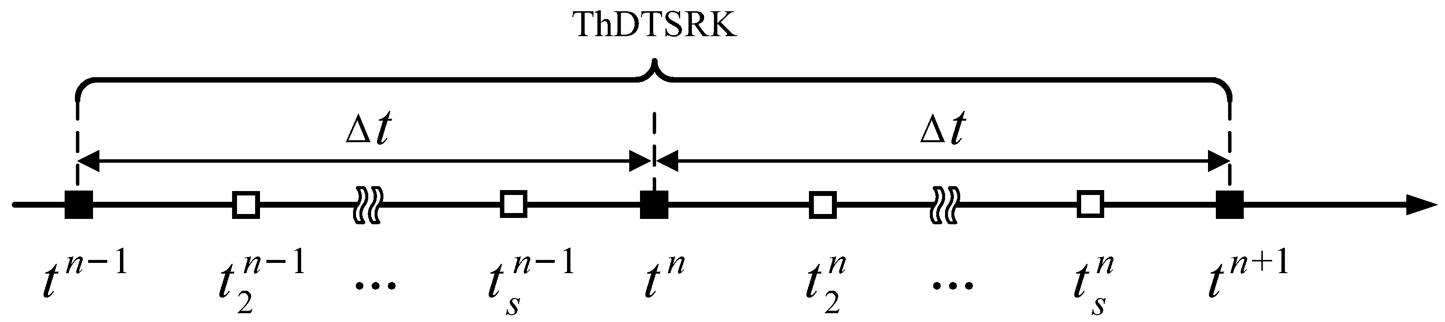
2. Structure of ThDTSRK Methods

We consider the ordinary differential equation as
y = F ( y ) ,
and the second and third derivatives are defined by
y = G ( y ) , y = H ( y ) .
The structure of s-stage ThDTSRK methods is depicted in Figure 1, and the fixed time step size Δ t is used to discretize the time interval. The explicit s-stage ThDTSRK schemes are given as follows:
Y i n 1 = y n 1 + Δ t j = 1 i 1 a i j F ( Y j n 1 ) + Δ t 2 j = 1 i 1 a ^ i j G ( Y j n 1 ) + Δ t 3 j = 1 i 1 a ¯ i j H ( Y j n 1 ) , Y i n = y n + Δ t j = 1 i 1 a i j F ( Y j n ) + Δ t 2 j = 1 i 1 a ^ i j G ( Y j n ) + Δ t 3 j = 1 i 1 a ¯ i j H ( Y j n ) , y n + 1 = ( 1 θ ) y n + θ y n 1 + Δ t i = 1 s v i F ( Y i n ) + w i F ( Y i n 1 ) + Δ t 2 i = 1 s v ^ i G ( Y i n ) + w ^ i G ( Y i n 1 ) + Δ t 3 i = 1 s v ¯ i H ( Y i n ) + w ¯ i H ( Y i n 1 ) ,
where y n 1 , y n , and y n + 1 are the solution values at time steps t n 1 , t n , t n + 1 , and Y i n 1 , and Y i n ( 2 i s ) denote the intermediate stage values at time steps t n 1 , t n . We also define first-stage values equal to the time step values Y 1 n 1 = y n 1 , Y 1 n = y n . The ThDTSRK methods can be rewritten in the matrix form
Y n 1 = e y n 1 + Δ t A F n 1 + Δ t 2 A ^ G n 1 + Δ t 3 A ¯ H n 1 , Y n = e y n + Δ t A F n + Δ t 2 A ^ G n + Δ t 3 A ¯ H n , y n + 1 = ( 1 θ ) y n + θ y n 1 + Δ t ( v T F n + w T F n 1 ) + Δ t 2 ( v ^ T G n + w ^ T G n 1 ) + Δ t 3 ( v ¯ T H n + w ¯ T H n 1 ) ,
where e is a vector of one, A is the RK matrix, A ^ is the TDRK matrix, and A ¯ is the ThDRK matrix. v , v ^ , v ¯ , w , w ^ , and w ¯ are weight vectors, and Y n 1 and Y n are vectors of time stage values, which are defined by
A = 0 0 0 a 21 0 0 a s 1 a s 2 0 , A ^ = 0 0 0 a ^ 21 0 0 a ^ s 1 a ^ s 2 0 , A ¯ = 0 0 0 a ¯ 21 0 0 a ¯ s 1 a ¯ s 2 0 , Y n 1 = Y 1 n 1 Y 2 n 1 Y s n 1 , Y n = Y 1 n Y 2 n Y s n , v = v 1 v 2 v s , v ^ = v ^ 1 v ^ 2 v ^ s , v ¯ = v ¯ 1 v ¯ 2 v ¯ s , w = w 1 w 2 w s , w ^ = w ^ 1 w ^ 2 w ^ s , w ¯ = w ¯ 1 w ¯ 2 w ¯ s .
The derivatives F n , F n 1 , G n , G n 1 H n , and H n 1 of the time stage vectors are defined by
F n = F ( Y 1 n ) F ( Y 2 n ) F ( Y s n ) , F n 1 = F ( Y 1 n 1 ) F ( Y 2 n 1 ) F ( Y s n 1 ) , G n = G ( Y 1 n ) G ( Y 2 n ) G ( Y s n ) , G n 1 = G ( Y 1 n 1 ) G ( Y 2 n 1 ) G ( Y s n 1 ) , H n = H ( Y 1 n ) H ( Y 2 n ) H ( Y s n ) , H n 1 = H ( Y 1 n 1 ) H ( Y 2 n 1 ) H ( Y s n 1 ) .
The size of the matrices is s × s and the size of the vectors is s × 1 . The time-levels for discretization methods are referred to as the abscissas c , which can be computed by c = A e . The ThDTSRK methods in Equation (3) can be represented by the extended Butcher tableau:
c A A ^ A ¯ v T v ^ T v ¯ T w T w ^ T w ¯ T

3. Order Conditions of ThDTSRK Methods

In this section, we develop a general form of the order accuracy conditions following Albrecht’s approach [10]; the detailed proof of order conditions for ThDTSRK methods is provided below.
First, the abscissas c are utilized to characterize the time stage vectors t n and t n 1 , and the expressions are given as t n = t n e + c Δ t and t n 1 = t n 1 e + c Δ t . By considering the truncation error τ n + 1 and stage truncation errors τ n and τ n 1 , the exact solution of ThDTSRK methods in Equation (4) can be expressed as follows:
Y ˜ n 1 = e y ˜ n 1 + Δ t A F ˜ n 1 + Δ t 2 A ^ G ˜ n 1 + Δ t 3 A ¯ H ˜ n 1 + τ n 1 , Y ˜ n = e y ˜ n + Δ t A F ˜ n + Δ t 2 A ^ G ˜ n + Δ t 3 A ¯ H ˜ n + τ n , y ˜ n + 1 = ( 1 θ ) y ˜ n + θ y ˜ n 1 + Δ t ( v T F ˜ n + w T F ˜ n 1 ) + Δ t 2 ( v ^ T G ˜ n + w ^ T G ˜ n 1 ) + Δ t 3 ( v ¯ T H ˜ n + w ¯ T H ˜ n 1 ) + τ n + 1 ,
where the tilde superscript denotes the exact values of the variables. Then, we expand truncation errors and exact stage values to the Taylor series expansions at the time step t n
τ n 1 = k = 1 τ k n 1 Δ t k y ˜ n ( k ) , τ n = k = 1 τ k n Δ t k y ˜ n ( k ) , τ n + 1 = k = 1 τ k n + 1 Δ t k y ˜ n ( k ) , Y ˜ i n 1 = k = 0 Δ t ( c i 1 ) k k ! y ˜ n ( k ) , Y ˜ i n = k = 0 Δ t k c i k k ! y ˜ n ( k ) , Y ˜ n + 1 = k = 0 Δ t k k ! y ˜ n ( k ) , F ( Y ˜ i n 1 ) = k = 1 Δ t ( c i 1 ) k 1 ( k 1 ) ! y ˜ n ( k ) , F ( Y ˜ i n ) = k = 1 Δ t k 1 c i k 1 ( k 1 ) ! y ˜ n ( k ) , G ( Y ˜ i n 1 ) = k = 2 Δ t ( c i 1 ) k 2 ( k 2 ) ! y ˜ n ( k ) , G ( Y ˜ i n ) = k = 2 Δ t k 2 c i k 2 ( k 2 ) ! y ˜ n ( k ) , H ( Y ˜ i n 1 ) = k = 3 Δ t ( c i 1 ) k 3 ( k 3 ) ! y ˜ n ( k ) , H ( Y ˜ i n ) = k = 3 Δ t k 3 c i k 3 ( k 3 ) ! y ˜ n ( k ) .
Taking Equation (7) into Equation (6), we obtain
τ k n = c k k ! A c k 1 ( k 1 ) ! A ^ c k 2 ( k 2 ) ! A ¯ c k 3 ( k 3 ) ! , τ k n + 1 = 1 θ ( 1 ) k k ! v T c k 1 ( k 1 ) ! w T ( c e ) k 1 ( k 1 ) ! v ^ T c k 2 ( k 2 ) ! w ^ T ( c e ) k 2 ( k 2 ) ! v ¯ T c k 3 ( k 3 ) ! w ¯ T ( c e ) k 3 ( k 3 ) ! .
The vectors Y ˜ n 1 , F ˜ n 1 , H ˜ n 1 and G ˜ n 1 can be expanded using Taylor series expansions at the time step t n 1 . By substituting these expansions into Equation (7), we can compute τ n 1 using the following expressions:
τ n 1 = k = 1 τ k n Δ t k y ˜ n 1 ( k ) .
The derivatives y ˜ n 1 ( k ) can be expanded by Taylor series expansions at the time step t n , and we have y ˜ n 1 ( k ) = m = 0 ( Δ t ) m m ! y ˜ n ( k + m ) , so the stage truncation errors τ k n 1 can be devised by
τ k n 1 = j = 1 k ( Δ t ) k j ( k j ) ! τ j n .
After determining the truncation error τ n + 1 and stage truncation errors τ n and τ n 1 , the subsequent task is to define the global error of the ThDTSRK methods by subtracting the exact value from the discretized numerical value. The specific procedure entails subtracting Equation (6) from Equation (4); we have
ϵ n 1 = e ϵ n 1 + Δ t A δ n 1 + Δ t 2 A ^ σ n 1 + Δ t 3 A ¯ η n 1 τ n 1 , ϵ n = e ϵ n + Δ t A δ n + Δ t 2 A ^ σ n + Δ t 3 A ¯ η n τ n , ϵ n + 1 = ( 1 θ ) ϵ n + θ ϵ n 1 + Δ t ( v T δ n + w T δ n 1 ) + Δ t 2 ( v ^ T σ n + w ^ T σ n 1 ) + Δ t 3 ( v ¯ T η n + w ¯ T η n 1 ) τ n + 1 ,
where the global error ϵ , the global stage errors ϵ , and the derivatives δ , σ , and η can be described as
ϵ = y y ˜ , ϵ = Y Y ˜ , δ = F F ˜ , σ = G G ˜ , η = H H ˜ .
The above global errors and derivatives are power series in Δ t :
ϵ n 1 = k = 1 p ϵ k n 1 Δ t k + O ( Δ t p + 1 ) , ϵ n = k = 1 p ϵ k n Δ t k + O ( Δ t p + 1 ) , δ n 1 = k = 1 p 1 δ k n 1 Δ t k + O ( Δ t p ) , δ n = k = 1 p 1 δ k n Δ t k + O ( Δ t p ) , σ n 1 = k = 1 p 2 σ k n 1 Δ t k + O ( Δ t p 1 ) , σ n = k = 1 p 2 σ k n Δ t k + O ( Δ t p 1 ) , η n 1 = k = 1 p 3 η k n 1 Δ t k + O ( Δ t p 2 ) , η n = k = 1 p 3 η k n Δ t k + O ( Δ t p 2 ) .
Substituting Equations (7) and (13) into Equation (11) yields
ϵ n 1 = e ϵ n 1 + k = 1 p 1 A δ k n 1 Δ t k + 1 + k = 1 p 2 A ^ σ k n 1 Δ t k + 2 + k = 1 p 3 A ¯ η k n 1 Δ t k + 3 k = 1 p τ k n 1 y ˜ n ( k ) Δ t k + e O ( Δ t p + 1 ) , ϵ n = e ϵ n + k = 1 p 1 A δ k n Δ t k + 1 + k = 1 p 2 A ^ σ k n Δ t k + 2 + k = 1 p 3 A ¯ η k n Δ t k + 3 k = 1 p τ k n y ˜ n ( k ) Δ t k + e O ( Δ t p + 1 ) , ϵ n + 1 = ( 1 θ ) ϵ n + θ ϵ n 1 + k = 1 p 1 ( v T δ k n + w T δ k n 1 ) Δ t k + 1 + k = 1 p 2 ( v ^ T σ k n + w ^ T σ k n 1 ) Δ t k + 2 + k = 1 p 3 ( v ¯ T η k n + w ¯ T η k n 1 ) Δ t k + 3 k = 1 p τ k n + 1 y ˜ n ( k ) Δ t k + O ( Δ t p + 1 ) .
Then, we analyze the global error ϵ n + 1 for the ThDTSRK methods. Since the previous time discretization format was the p-order accuracy method, we can deduce the p-order conditions for the ThDTSRK methods:
τ k n + 1 = 0 , v T δ k 1 n + w T δ k 1 n 1 = 0 , v ^ T σ k 2 n + w ^ T σ k 2 n 1 = 0 , v ¯ T η k 3 n + w ¯ T η k 3 n 1 = 0 .
To complete the order conditions for the ThDTSRK methods, we need to establish the vectors δ k , σ k , and η k . Indeed, these vectors can be recursively derived from the global stage errors ϵ . By employing the Taylor series expansions at the exact stage values y ˜ , the interrelation between the derivatives and the global stage errors of derivatives can be revealed as
F = F ˜ + j = 1 1 j ! ( ϵ ) j · F ˜ ( j ) G = G ˜ + j = 1 1 j ! ( ϵ ) j · G ˜ ( j ) H = H ˜ + j = 1 1 j ! ( ϵ ) j · H ˜ ( j ) δ = F F ˜ = j = 1 1 j ! ( ϵ ) j · F ˜ ( j ) σ = G G ˜ = j = 1 1 j ! ( ϵ ) j · G ˜ ( j ) η = H H ˜ = j = 1 1 j ! ( ϵ ) j · H ˜ ( j )
Here, the dot product represents component-wise multiplication, and the vectors of derivations are given as
F ˜ ( j ) = j F ( Y ˜ 1 ) ( Y ˜ 1 ) j , j F ( Y ˜ 2 ) ( Y ˜ 2 ) j , , j F ( Y ˜ s ) ( Y ˜ s ) j T , G ˜ ( j ) = j G ( Y ˜ 1 ) ( Y ˜ 1 ) j , j G ( Y ˜ 2 ) ( Y ˜ 2 ) j , , j G ( Y ˜ s ) ( Y ˜ s ) j T , H ˜ ( j ) = j H ( Y ˜ 1 ) ( Y ˜ 1 ) j , j H ( Y ˜ 2 ) ( Y ˜ 2 ) j , , j H ( Y ˜ s ) ( Y ˜ s ) j T .
Similarly, we derive expressions for F ˜ ( j ) , G ˜ ( j ) , and H ˜ ( j ) of Equation (16) by employing the Taylor series expansions at time step t n
F ˜ n 1 ( j ) = l = 0 Δ t l l ! ( c e ) l · F ˜ n ( j , l ) , F ˜ n ( j ) = l = 0 Δ t l l ! c l · F ˜ n ( j , l ) , G ˜ n 1 ( j ) = l = 0 Δ t l l ! ( c e ) l · G ˜ n ( j , l ) , G ˜ n ( j ) = l = 0 Δ t l l ! c l · G ˜ n ( j , l ) , H ˜ n 1 ( j ) = l = 0 Δ t l l ! ( c e ) l · H ˜ n ( j , l ) , H ˜ n ( j ) = l = 0 Δ t l l ! c l · H ˜ n ( j , l ) ,
where the vector of derivation is as follows:
F ˜ ( j , l ) = j + l F ( Y ˜ 1 ) ( Y ˜ 1 ) j ( t n ) l , j + l F ( Y ˜ 2 ) ( Y ˜ 2 ) j ( t n ) l , , j + l F ( Y ˜ s ) ( Y ˜ s ) j ( t n ) l T , G ˜ ( j , l ) = j + l G ( Y ˜ 1 ) ( Y ˜ 1 ) j ( t n ) l , j + l G ( Y ˜ 2 ) ( Y ˜ 2 ) j ( t n ) l , , j + l G ( Y ˜ s ) ( Y ˜ s ) j ( t n ) l T , H ˜ ( j , l ) = j + l H ( Y ˜ 1 ) ( Y ˜ 1 ) j ( t n ) l , j + l H ( Y ˜ 2 ) ( Y ˜ 2 ) j ( t n ) l , , j + l H ( Y ˜ s ) ( Y ˜ s ) j ( t n ) l T .
According to Equations (16) and (17), we ultimately deduce the intended expansion:
δ n 1 = j = 1 l = 0 Δ t l j ! l ! C ¯ l ( ϵ n 1 ) j · F ˜ n ( j , l ) , δ n = j = 1 l = 0 Δ t l j ! l ! C l ( ϵ n ) j · F ˜ n ( j , l ) , σ n 1 = j = 1 l = 0 Δ t l j ! l ! C ¯ l ( ϵ n 1 ) j · G ˜ n ( j , l ) , σ n = j = 1 l = 0 Δ t l j ! l ! C l ( ϵ n ) j · G ˜ n ( j , l ) , η n 1 = j = 1 l = 0 Δ t l j ! l ! C ¯ l ( ϵ n 1 ) j · H ˜ n ( j , l ) , η n = j = 1 l = 0 Δ t l j ! l ! C l ( ϵ n ) j · H ˜ n ( j , l ) ,
where C and C ¯ are diagonal matrices composed of vectors c and c e .
Finally, the terms of vectors δ , σ , η , and ϵ are provided in Appendix A. Based on Equation (15), the order conditions for the ThDTSRK schemes are presented in Table 1. Moreover, further information can be obtained from our source code [19].

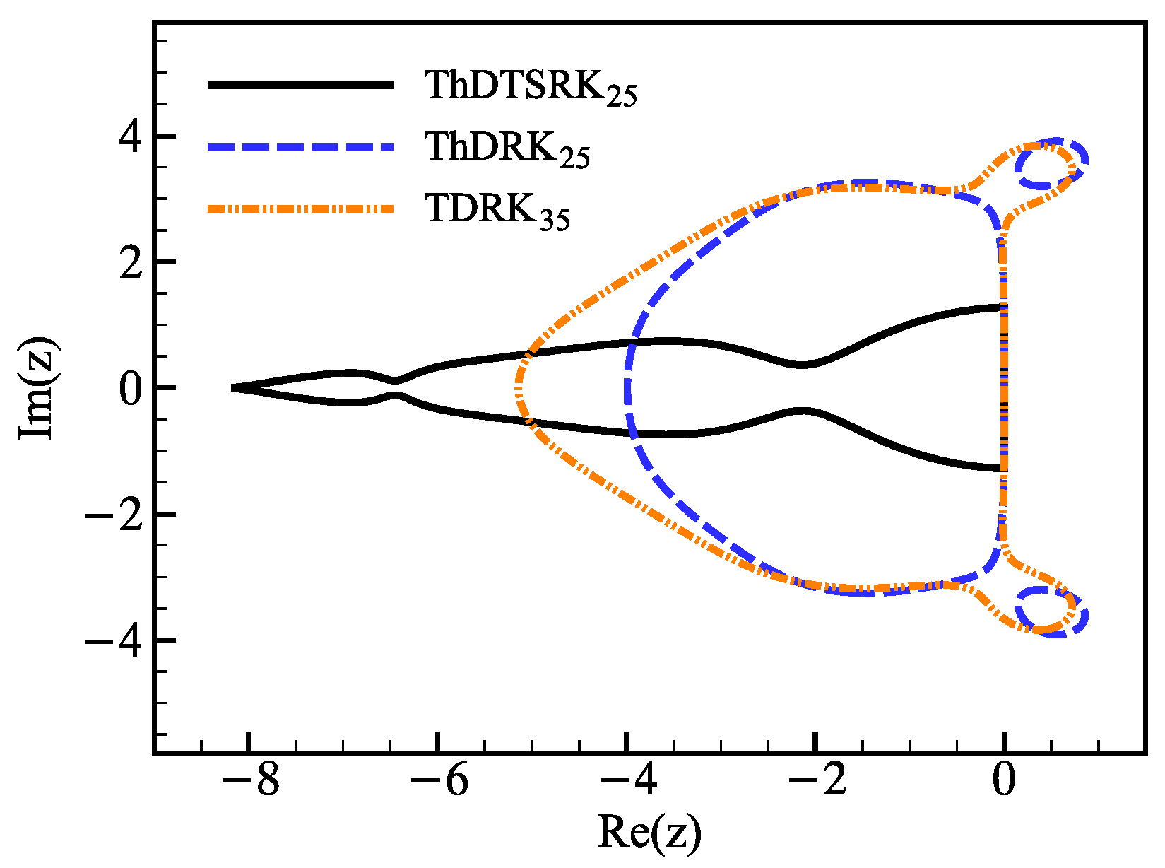
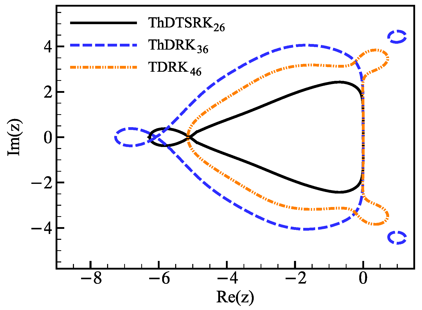
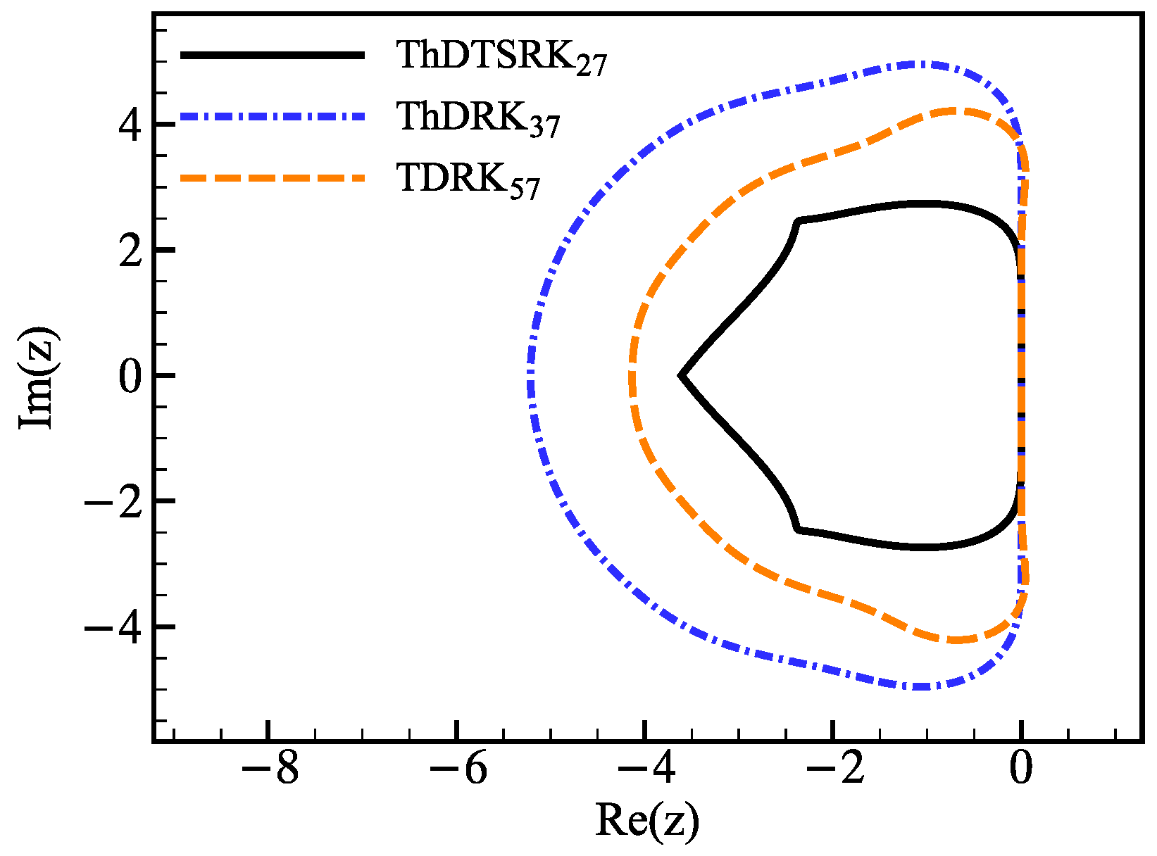
4. Stability Analysis

4.1. A-Stability Property

To investigate the A-stability property of the ThDTSRK methods, the classical test equation y = λ y is utilized, where λ is a complex parameter. The ThDTSRK methods in Equation (4) can be expressed in a compact matrix form:
T y n + 1 = A 1 B 1 C 1 D 1 A 2 B 2 C 2 D 2 Δ t F ( T ) Δ t 2 G ( T ) Δ t 3 H ( T ) y n ,
where the vectors T , y n , and y n + 1 are specified by
T = Y n 1 Y n , y n = Y n 1 y n 1 y n , y n + 1 = Y n y n y n + 1 ,
and the matrices A 1 , A 2 , B 1 , B 2 , C 1 , C 2 , D 1 , D 2 are given by
A 1 = A 0 0 A , B 1 = A ^ 0 0 A ^ , C 1 = A ¯ 0 0 A ¯ , D 1 = 0 e 0 0 0 e , A 2 = 0 A 0 0 w T v T , B 2 = 0 A ^ 0 0 w ^ T v ^ T , C 2 = 0 A ¯ 0 0 w ¯ T v ¯ T , D 2 = 0 s × s 0 s × 1 e 0 1 × s 0 1 0 1 × s θ 1 θ .
Based on the stability theory for TSRK schemes [20], the recurrence relation can be given by y n + 1 = M ( z ) y n and the stability matrix M ( z ) can be determined as
M ( z ) = D 2 + z A 2 + z 2 B 2 + z 3 C 2 I 2 s z A 1 z 2 B 1 z 3 C 1 1 D 1 ,
where z = λ Δ t , and the stability polynomial f ( α , z ) of the ThDTSRK schemes Equation (19) is defined by
f ( α , z ) = d e t α I s + 2 M ( z ) .
Then, we compute the roots of equation f ( α , z ) = 0 and obtain the expression of the roots as α = g ( z ) . The region of absolute stability D is the definition that all roots are inside the unit circle; we have
D = { z C : α k = g k ( z ) < 1 , k = 1 , 2 , , s + 2 } .

4.2. Optimal ThDTSRK Schemes

By employing stability theory, A-stability preserving ThDTSRK s p methods have been proposed, in which the subscript denotes the p-order scheme with s-stage. Here, we display the ThDTSRK schemes with two stages; the stability polynomial f ( α , z ) is expressed as
f ( α , z ) = α 2 α 2 φ 1 α φ 2 , φ 1 = 1 + ( v 1 + v 2 ) z + ( a 21 v 2 + v ^ 1 + v ^ 2 ) z 2 + ( 1 2 a 21 2 v 2 + a 21 v ^ 2 + v ¯ 1 + v ¯ 2 ) z 3 + ( 1 6 a 21 3 v 2 + 1 2 a 21 2 v ^ 2 + a 21 v ¯ 2 ) z 4 + ( 1 6 a 21 3 v ^ 2 + 1 2 a 21 2 v ¯ 2 ) z 5 + 1 6 a 21 3 v ¯ 2 z 6 θ , φ 2 = ( w 1 + w 2 ) z + ( a 21 w 2 + w ^ 1 + w ^ 2 ) z 2 + ( 1 2 a 21 2 w 2 + a 21 w ^ 2 + w ¯ 1 + w ¯ 2 ) z 3 + ( 1 6 a 21 3 w 2 + 1 2 a 21 2 w ^ 2 + a 21 w ¯ 2 ) z 4 + ( 1 6 a 21 3 w ^ 2 + 1 2 a 21 2 w ¯ 2 ) z 5 + 1 6 a 21 3 w ¯ 2 z 6 + θ .
Next, we calculate the roots of equation f ( α , z ) = 0 and the expression of the roots is shown as
α 1 = 1 2 ( φ 1 + φ 1 2 + 4 φ 2 ) , α 2 = 1 2 ( φ 1 φ 1 2 + 4 φ 2 ) , α 3 = 0 , α 4 = 0 .
Utilizing Equations (24) and (26), we can obtain the region of absolute stability and determine the optimal corresponding parameters for the ThDTSRK schemes. The aim of this optimization process is to construct ThDTSRK methods with large region intervals [ L , 0 ] of absolute stability. Here, we define the intersection L of the absolute stability region with the negative real line. Similarly to the authors of reference [21], this will be carried out by solving the optimization problem to find the optimal ThDTSRK schemes with the largest value of | L | .
(1) 
Two-Stage Fifth-Order ThDTSRK Scheme (ThDTSRK 25 )
The coefficients of the general two-stage fifth-order ThDTSRK method are then given as a eight-parameter system, depending on θ , a 21 , w 1 , w 2 , v ^ 2 , w ^ 2 , v ¯ 2 , w ¯ 2 , which are related through
v 1 = 1 w 1 + θ ; v 2 = w 2 ; a ^ 21 = a 21 2 / 2 ; a ¯ 21 = a 21 3 / 6 ; v ^ 1 = ( 3 20 v ^ 2 + 60 a 21 2 v ^ 2 + 40 a 21 3 v ^ 2 + 120 a 21 v ¯ 2 + 120 a 21 2 v ¯ 2 + 10 w 1 + 10 w 2 + 20 a 21 w 2 40 a 21 3 w 2 60 a 21 2 w ^ 2 + 40 a 21 3 w ^ 2 120 a 21 w ¯ 2 + 120 a 21 2 w ¯ 2 7 θ ) / 20 ; w ^ 1 = ( 1 θ ) / 2 + w 1 + w 2 v ^ 1 v ^ 2 w ^ 2 ; v ¯ 1 = ( 23 60 a 21 v ^ 2 120 a 21 2 v ^ 2 60 a 21 3 v ^ 2 60 v ¯ 2 240 a 21 v ¯ 2 180 a 21 2 v ¯ 2 5 w 1 5 w 2 + 30 a 21 2 w 2 + 60 a 21 3 w 2 + 60 a 21 2 w ^ 2 60 a 21 3 w ^ 2 + 120 a 21 w ¯ 2 180 a 21 2 w ¯ 2 + 3 θ ) / 60 ; w ¯ 1 = ( 8 60 a 21 2 v ^ 2 60 a 21 3 v ^ 2 120 a 21 v ¯ 2 180 a 21 2 v ¯ 2 + 5 w 1 + 5 w 2 30 a 21 2 w 2 + 60 a 21 3 w 2 60 a 21 w ^ 2 + 120 a 21 2 w ^ 2 60 a 21 3 w ^ 2 60 w ¯ 2 + 240 a 21 w ¯ 2 180 a 21 2 w ¯ 2 2 θ ) / 60 .
The coefficients matrices of the optimal ThDTSRK 25 scheme are derived by
θ = 0 , c = c 1 c 2 = 0 0.1983891070202614 , A = 0 0 c 2 0 , A ^ = 0 0 c 2 2 2 0 , A ¯ = 0 0 c 2 3 6 0 , v T = 0.4988123289876567 0.1677439748133182 , w T = 0.5011876710123433 0.1677439748133182 , v ^ T = 0.0958493173039603 0.6579633161995648 , w ^ T = 0.8843764374259575 1.4911940843560145 , v ¯ T = 0.0202481631489146 0.1199846505868748 , w ¯ T = 0.1160041365433313 0.0621952996182998 .
(2) 
Two-Stage Sixth-Order ThDTSRK Scheme (ThDTSRK26)
The coefficients of the general two-stage sixth-order ThDTSRK method are then given as a five-parameter system, depending on θ , a 21 , w ^ 2 , v ¯ 2 , w ¯ 2 , which are related through
v 2 = 0 ; w 2 = 0 ; v ^ 2 = w ^ 2 ; a ^ 21 = a 21 2 / 2 ; a ¯ 21 = a 21 3 / 6 ; v 1 = ( 15 120 a 21 v ¯ 2 360 a 21 2 v ¯ 2 240 a 21 3 v ¯ 2 + 240 a 21 3 w ^ 2 120 a 21 w ¯ 2 + 360 a 21 2 w ¯ 2 240 a 21 3 w ¯ 2 + θ ) / 2 ; w 1 = 1 + θ v 1 ; v ^ 1 = ( 31 + 360 a 21 v ¯ 2 + 960 a 21 2 v ¯ 2 + 600 a 21 3 v ¯ 2 + 10 w ^ 2 60 a 21 2 w ^ 2 600 a 21 3 w ^ 2 + 240 a 21 w ¯ 2 840 a 21 2 w ¯ 2 + 600 a 21 3 w ¯ 2 θ ) / 10 ; w ^ 1 = ( 29 + 240 a 21 v ¯ 2 + 840 a 21 2 v ¯ 2 + 600 a 21 3 v ¯ 2 10 w ^ 2 + 60 a 21 2 w ^ 2 600 a 21 3 w ^ 2 + 360 a 21 w ¯ 2 960 a 21 2 w ¯ 2 + 600 a 21 3 w ¯ 2 + θ ) / 10 ; v ¯ 1 = ( 111 120 v ¯ 2 1080 a 21 v ¯ 2 2160 a 21 2 v ¯ 2 1200 a 21 3 v ¯ 2 + 120 a 21 w ^ 2 + 360 a 21 2 w ^ 2 + 1200 a 21 3 w ^ 2 360 a 21 w ¯ 2 + 1440 a 21 2 w ¯ 2 1200 a 21 3 w ¯ 2 + θ ) / 120 ; w ¯ 1 = ( 49 + 360 a 21 v ¯ 2 + 1440 a 21 2 v ¯ 2 + 1200 a 21 3 v ¯ 2 120 a 21 w ^ 2 + 360 a 21 2 w ^ 2 1200 a 21 3 w ^ 2 120 w ¯ 2 + 1080 a 21 w ¯ 2 2160 a 21 2 w ¯ 2 + 1200 a 21 3 w ¯ 2 + θ ) / 120 .
The coefficients matrices of the optimal ThDTSRK 26 scheme are given by
θ = 0 , c = c 1 c 2 = 0 0.5873258965737987 , A = 0 0 c 2 0 , A ^ = 0 0 c 2 2 2 0 , A ¯ = 0 0 c 2 3 6 0 , v T = 1.0471220060600115 0 , w T = 0.0471220060600116 0 , v ^ T = 0.4467995963745828 0.1411691523070592 , w ^ T = 0.0060783975654054 0.1411691523070592 , v ¯ T = 0.0482868172625281 0.0243580486114999 , w ¯ T = 0.0052528132887524 0.0227607642077618 .
(3) 
Two-Stage Seventh-Order ThDTSRK Scheme (ThDTSRK27)
The coefficients of the general two-stage seventh-order ThDTSRK method are then given as a two-parameter system, depending only on θ , a 21 , which are related through
v 2 = 0 ; w 2 = 0 ; v ^ 2 = 0 ; w ^ 2 = 0 ; a ^ 21 = a 21 2 / 2 ; a ¯ 21 = a 21 3 / 6 ; v 1 = ( 105 627 a 21 + 1050 a 21 2 + 7 θ + 3 a 21 θ + 70 a 21 2 θ ) / ( 14 ( 1 + 10 a 21 2 ) ) ; w 1 = ( 91 + 627 a 21 910 a 21 2 + 7 θ 3 a 21 θ + 70 a 21 2 θ ) / ( 14 ( 1 + 10 a 21 2 ) ) ; v ^ 1 = ( 45 + 627 a 21 868 a 21 2 3 θ 3 a 21 θ 28 a 21 2 θ ) / ( 28 ( 1 + 10 a 21 2 ) ) ; w ^ 1 = ( 123 + 627 a 21 812 a 21 2 + 3 θ 3 a 21 θ + 28 a 21 2 θ ) / ( 28 ( 1 + 10 a 21 2 ) ) ; v ¯ 1 = ( 209 + 300 a 21 6270 a 21 2 + 15540 a 21 3 + θ + 20 a 21 θ + 30 a 21 2 θ + 140 a 21 3 θ ) / ( 1680 ( a 21 + 10 a 21 3 ) ) ; v ¯ 2 = ( 209 θ ) / ( 1680 ( a 21 + 10 a 21 3 ) ) ; w ¯ 2 = v ¯ 2 ; w ¯ 1 = ( 209 1940 a 21 + 6270 a 21 2 6860 a 21 3 θ + 20 a 21 θ 30 a 21 2 θ + 140 a 21 3 θ ) / ( 1680 ( a 21 + 10 a 21 3 ) ) .
The coefficient matrices of the optimal ThDTSRK 27 scheme are obtained by
θ = 0 , c = c 1 c 2 = 0 1 2 , A = 0 0 c 2 0 , A ^ = 0 0 c 2 2 2 0 , A ¯ = 0 0 c 2 3 6 0 , v T = 54 49 0 , w T = 5 49 0 , v ^ T = 103 196 0 , w ^ T = 25 196 0 , v ¯ T = 79 735 209 2940 , w ¯ T = 17 980 209 2940 .
To evaluate the performance of the designed methods, a comparison was conducted between high-order ThDTSRK methods, TDRK methods [13], and ThDRK methods [14]. The absolute stability regions of high-order ThDTSRK methods are displayed in Figure 2, Figure 3 and Figure 4. We define the scaled intersection L * of absolute stability, which is derived by
L * = p γ s L ,
where γ = 2 for two-derivative schemes and γ = 3 for three-derivative schemes. In Table 2, the results indicate that the ThDTSRK methods exhibit a larger scaled intersection L * compared to other schemes of the same order.

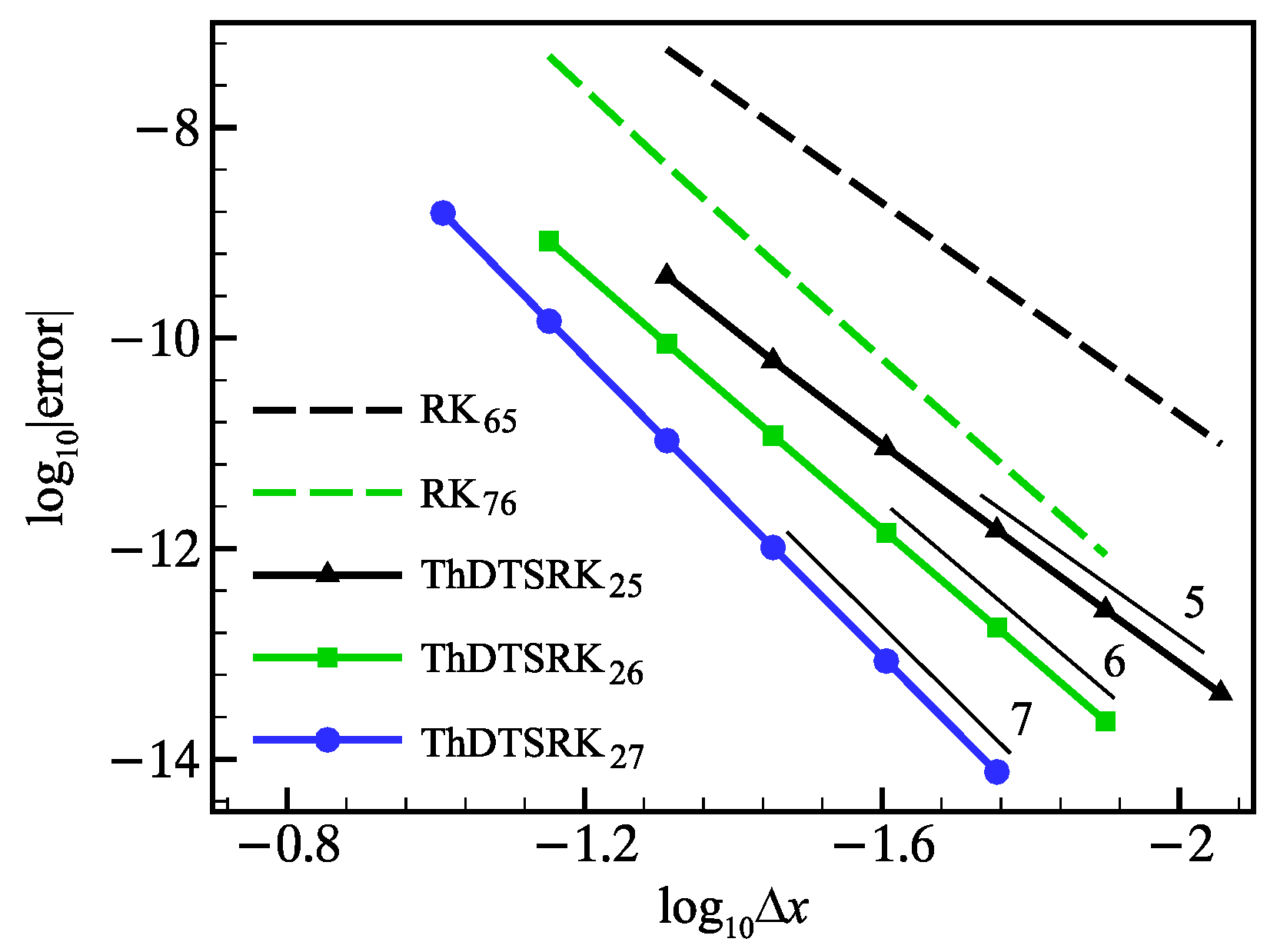
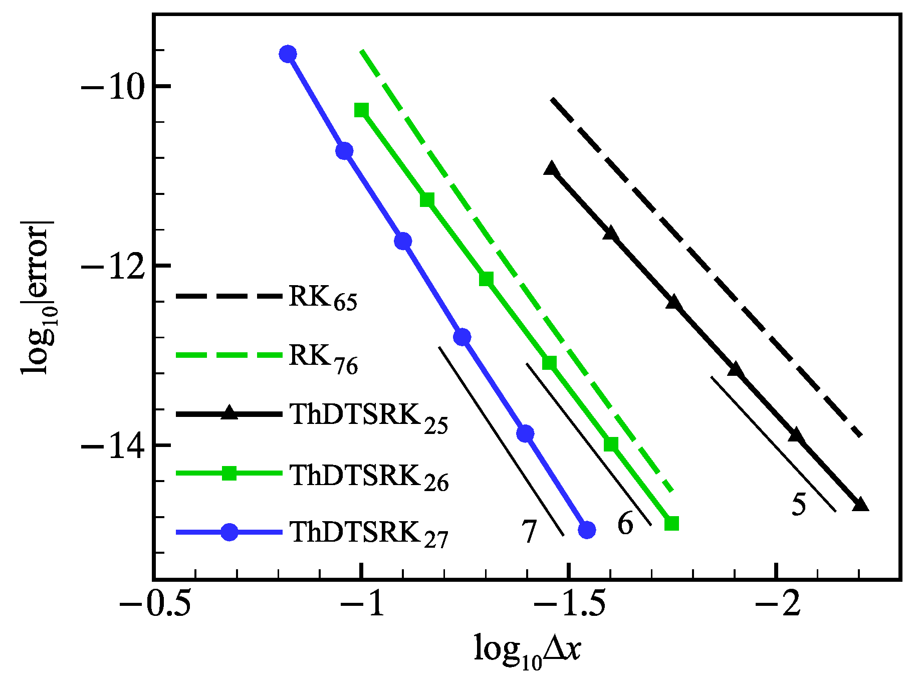
5. Numerical Examples

5.1. Prothero–Robinson Problem

We test the order accuracy of ThDTSRK methods using the Prothero–Robinson problem [13], which is expressed as
y ( x ) = λ ( y ( x ) sin ( x ) ) + cos ( x ) , λ = 10 .
The exact solution is given by y ( x ) = sin ( x ) and the results are integrated to 2.8 π . In Figure 5, the results clearly demonstrate that the ThDTSRK methods attain the desired order accuracy. Additionally, the ThDTSRK methods are more efficient than the classical high-order Runge–Kutta methods [11,13].

5.2. Kaps Problem

We test the order accuracy of ThDTSRK methods employing the Kaps problem [13], which is expressed as
y ( x ) = y 1 1 + y 1 + y 2 λ y 1 2 y 2 2 y 2 , y ( 0 ) = 1 1 , λ = 10 .
The exact result is y ( x ) = [ e ( x ) , e ( 2 x ) ] , and the solutions integrated up to five are presented in Figure 6. These results also reveal that the ThDTSRK methods attain the designed order accuracy. The ThDTSRK methods are more efficient compared with the classical high-order Runge–Kutta methods in solving ordinary differential equations.

6. Conclusions

In this study, we developed the order conditions for the ThDTSRK schemes that ensure these methods can achieve theoretical order accuracy. The parameters of the general high-order ThDTSRK methods were provided by utilizing the order conditions. Additionally, we established the A-stability property theory for ThDTSRK methods to determine the optimal stability coefficients. By comparing the ThDTSRK methods with ThDRK and TDRK schemes, the results revealed that the ThDTSRK schemes can maintain the A-stability property and attain the desired order accuracy while utilizing fewer stages. This indicates that the ThDTSRK methods are computationally efficient for solving ordinary differential equations. In further studies, our proposed ThDTSRK schemes can be applied to partial differential equations which are reduced to ordinary differential equation system using various spatial discretization schemes [5,22]. The TDMSRK methods can demonstrate high computational efficiency, especially when employing high-order spatial discretization schemes.

Author Contributions

Writing—original draft, X.Q.; Writing—review & editing, J.Y. and C.Y. All authors have read and agreed to the published version of the manuscript.

Funding

This study was supported by the Fundamental Research Funds for the Central Universities.

Data Availability Statement

The data and code are available in our open-source repository [19].

Conflicts of Interest

The authors declare no conflicts of interest.

Appendix A. Order Conditions for ThDTSRK Schemes

First-order:
Condition: τ 1 n + 1 = 0
Second-order:
Terms ϵ 1 n : 0
δ 1 n : 0
ϵ 1 n 1 : 0
δ 1 n 1 : 0
Condition: τ 2 n + 1 = 0
Third-order:
Terms ϵ 2 n : τ 2 n
δ 2 n : τ 2 n
σ 1 n : 0
ϵ 2 n 1 : τ 2 n 1
δ 2 n 1 : τ 2 n 1
σ 1 n 1 : 0
Condition: τ 3 n + 1 = 0 , v T τ 2 n + w T τ 2 n 1 = 0
Fourth-order:
Terms: ϵ 3 n : A τ 2 n , τ 3 n
δ 3 n : C τ 2 n , A τ 2 n , τ 3 n
σ 2 n : τ 2 n
η 1 n : 0 .
ϵ 3 n 1 : A τ 2 n 1 , τ 3 n 1
δ 3 n 1 : C ¯ τ 2 n 1 , A τ 2 n 1 , τ 3 n 1
σ 2 n 1 : τ 2 n 1
η 1 n 1 : 0 .
Condition: τ 4 n + 1 = 0 , v T C τ 2 n + w T C ¯ τ 2 n 1 = 0 , v T A τ 2 n + w T A τ 2 n 1 = 0 , v T τ 3 n + w T τ 3 n 1 = 0 , v ^ T τ 2 n + w ^ T τ 2 n 1 = 0
Fifth-order:
Terms: ϵ 4 n : A τ 3 n , τ 4 n
δ 4 n : C τ 3 n , A τ 3 n , τ 4 n
σ 3 n : τ 3 n
η 1 n : 0 .
ϵ 4 n 1 : A τ 3 n 1 , τ 4 n 1
δ 4 n 1 : C ¯ τ 3 n 1 , A τ 3 n 1 , τ 4 n 1
σ 3 n 1 : τ 3 n 1
η 1 n 1 : 0 .
Condition: τ 5 n + 1 = 0 , τ 2 n = 0 , v T C τ 3 n + w T C ¯ τ 3 n 1 = 0 , v T A τ 3 n + w T A τ 3 n 1 = 0 , v ^ T τ 3 n + w ^ T τ 3 n 1 = 0 , v T τ 4 n + w T τ 4 n 1 = 0
Sixth-order:
Terms: ϵ 5 n : A C τ 3 n , A 2 τ 3 n , A ^ τ 3 n , A τ 4 n , τ 5 n
δ 5 n : C 2 τ 3 n , C A τ 3 n , C τ 4 n , ϵ 5 n
σ 4 n : C τ 3 n , A τ 3 n , τ 4 n
η 3 n : τ 3 n .
ϵ 5 n 1 : A C ¯ τ 3 n 1 , A 2 τ 3 n 1 , A ^ τ 3 n 1 , A τ 4 n 1 , τ 5 n 1
δ 5 n 1 : C ¯ 2 τ 3 n 1 , C ¯ A τ 3 n 1 , C ¯ τ 4 n 1 , ϵ 5 n 1
σ 4 n 1 : C ¯ τ 3 n 1 , A τ 3 n 1 , τ 4 n 1
η 3 n 1 : τ 3 n 1 .
Condition: τ 6 n + 1 = 0 , v T A 2 τ 3 n + w T A 2 τ 3 n 1 = 0 , v T C A τ 3 n + w T C ¯ A τ 3 n 1 = 0 , v T A C τ 3 n + w T A C ¯ τ 3 n 1 = 0 , v T C 2 τ 3 n + w T C ¯ 2 τ 3 n 1 = 0 , v T A ^ τ 3 n + w T A ^ τ 3 n 1 = 0 , v ^ T A τ 3 n + w ^ T A τ 3 n 1 = 0 , v ^ T C τ 3 n + w ^ T C ¯ τ 3 n 1 = 0 , v ¯ T τ 3 n + w ¯ T τ 3 n 1 = 0 , v T C τ 4 n + w T C ¯ τ 4 n 1 = 0 , v T A τ 4 n + w T A τ 4 n 1 = 0 , v ^ T τ 4 n + w ^ T τ 4 n 1 = 0 , v T τ 5 n + w T τ 5 n 1 = 0
Seventh-order:
Terms: ϵ 6 n : A C τ 4 n , A 2 τ 4 n , A ^ τ 4 n , A τ 5 n , τ 6 n
δ 6 n : C 2 τ 4 n , C A τ 4 n , C τ 5 n , ϵ 6 n
σ 5 n : C τ 4 n , A τ 4 n , τ 5 n
η 4 n : τ 4 n .
ϵ 6 n 1 : A C ¯ τ 4 n 1 , A 2 τ 4 n 1 , A ^ τ 4 n 1 , A τ 5 n 1 , τ 6 n 1
δ 6 n 1 : C ¯ 2 τ 4 n 1 , C ¯ A τ 4 n 1 , C ¯ τ 5 n 1 , ϵ 6 n 1
σ 5 n 1 : C ¯ τ 4 n 1 , A τ 4 n 1 , τ 5 n 1
η 4 n 1 : τ 4 n 1 .
Condition: τ 7 n + 1 = 0 , τ 3 n = 0 , v T A 2 τ 4 n + w T A 2 τ 4 n 1 = 0 , v T A C τ 4 n + w T A C ¯ τ 4 n 1 = 0 , v T C A τ 4 n + w T C ¯ A τ 4 n 1 = 0 , v T C 2 τ 4 n + w T C ¯ 2 τ 4 n 1 = 0 , v T A ^ τ 4 n + w T A ^ τ 4 n 1 = 0 , v ^ T A τ 4 n + w ^ T A τ 4 n 1 = 0 , v ^ T C τ 4 n + w ^ T C ¯ τ 4 n 1 = 0 , v ¯ T τ 4 n + w ¯ T τ 4 n 1 = 0 , v T A τ 5 n + w T A τ 5 n 1 = 0 , v T C τ 5 n + w T C ¯ τ 5 n 1 = 0 , v ^ T τ 5 n + w ^ T τ 5 n 1 = 0 , v T τ 6 n + w T τ 6 n 1 = 0

References

  1. Dormand, J.R.; Prince, P.J. A family of embedded Runge-Kutta formulae. J. Comput. Appl. Math. 1980, 6, 19–26. [Google Scholar] [CrossRef]
  2. Kovalnogov, V.N.; Fedorov, R.V.; Karpukhina, T.V.; Simos, T.E.; Tsitouras, C. On Reusing the Stages of a Rejected Runge-Kutta Step. Mathematics 2023, 11, 2589. [Google Scholar] [CrossRef]
  3. Kovalnogov, V.N.; Fedorov, R.V.; Chukalin, A.V.; Simos, T.E.; Tsitouras, C. Evolutionary Derivation of Runge–Kutta Pairs of Orders 5(4) Specially Tuned for Problems with Periodic Solutions. Mathematics 2021, 9, 2306. [Google Scholar] [CrossRef]
  4. Verner, J. High-order explicit Runge-Kutta pairs with low stage order. Appl. Numer. Math. 1996, 22, 345–357. [Google Scholar] [CrossRef]
  5. Qin, X.; Jiang, Z.; Yu, J.; Huang, L.; Yan, C. Strong stability-preserving three-derivative Runge–Kutta methods. Comput. Appl. Math. 2023, 42, 171. [Google Scholar] [CrossRef]
  6. Wen, J.; Xiao, A.; Huang, C. Highly stable multistep Runge–Kutta methods for Volterra integral equations. Comput. Appl. Math. 2020, 39, 308. [Google Scholar] [CrossRef]
  7. Moradi, A.; Abdi, A.; Hojjati, G. RK-stable second derivative multistage methods with strong stability preserving based on Taylor series conditions. Comput. Appl. Math. 2023, 42, 193. [Google Scholar] [CrossRef]
  8. Butcher, J.C. An algebraic theory of integration methods. Math. Comput. 1972, 26, 79–106. [Google Scholar] [CrossRef]
  9. Butcher, J.C. Trees and numerical methods for ordinary differential equations. Numer. Algor. 2010, 53, 153–170. [Google Scholar] [CrossRef]
  10. Albrecht, P. The Runge-Kutta theory in a nutshell. SIAM J. Numer. Anal. 1996, 33, 1712–1735. [Google Scholar] [CrossRef]
  11. Butcher, J.C. Numerical Methods for Ordinary Differential Equations; John Wiley & Sons: Hoboken, NJ, USA, 2016; pp. 243–267. [Google Scholar] [CrossRef]
  12. Butcher, J.C.; Hojjati, G. Second derivative methods with RK stability. Numer. Algor. 2005, 40, 415–429. [Google Scholar] [CrossRef]
  13. Chan, R.P.; Tsai, A.Y. On explicit two-derivative Runge-Kutta methods. Numer. Algor. 2010, 53, 171–194. [Google Scholar] [CrossRef]
  14. Turacı, M.Ö.; Öziş, T. Derivation of three-derivative Runge-Kutta methods. Numer. Algor. 2017, 74, 247–265. [Google Scholar] [CrossRef]
  15. Ketcheson, D.I.; Gottlieb, S.; Macdonald, C.B. Strong stability preserving two-step Runge–Kutta methods. SIAM J. Numer. Anal. 2011, 49, 2618–2639. [Google Scholar] [CrossRef]
  16. Ökten Turaci, M.; Öziş, T. On explicit two-derivative two-step Runge–Kutta methods. Comput. Appl. Math. 2018, 37, 6920–6954. [Google Scholar] [CrossRef]
  17. Bresten, C.; Gottlieb, S.; Grant, Z.; Higgs, D.; Ketcheson, D.; Németh, A. Explicit strong stability preserving multistep Runge-Kutta methods. Math. Comput. 2017, 86, 747–769. [Google Scholar] [CrossRef]
  18. Enright, W. Second derivative multistep methods for stiff ordinary differential equations. SIAM J. Numer. Anal. 1974, 11, 321–331. [Google Scholar] [CrossRef]
  19. Explicit Three-Derivative Two-Step Runge-Kutta Methods Code. 2023. Available online: https://github.com/aerfa-buaa/Explicit-Three-Derivative-Two-Step-Runge-Kutta-Methods-ThDTSRK (accessed on 1 October 2023).
  20. Bartoszewski, Z.; Jackiewicz, Z. Construction of two-step Runge-Kutta methods of high order for ordinary differential equations. Numer. Algor. 1998, 18, 51–70. [Google Scholar] [CrossRef]
  21. Figueroa, A.; Jackiewicz, Z.; Löhner, R. Efficient two-step Runge-Kutta methods for fluid dynamics simulations. Appl. Numer. Math. 2021, 159, 1–20. [Google Scholar] [CrossRef]
  22. Zorío, D.; Baeza, A.; Mulet, P. An approximate Lax–Wendroff-type procedure for high order accurate schemes for hyperbolic conservation laws. J. Sci. Comput. 2017, 71, 246–273. [Google Scholar] [CrossRef]
Figure 1. The structure of the s-stage ThDTSRK methods. (The solid square represents time step, and the hollow square represents time stage).
Mathematics 12 00711 g001
Figure 2. The stability regions of different fifth-order schemes, including the ThDTSRK scheme, ThDRK scheme, and TDRK scheme.
Mathematics 12 00711 g002
Figure 3. The stability regions of different sixth-order schemes, including the ThDTSRK scheme, ThDRK scheme, and TDRK scheme.
Mathematics 12 00711 g003
Figure 4. The stability regions of different seventh-order schemes, including the ThDTSRK scheme, ThDRK scheme, and TDRK scheme.
Mathematics 12 00711 g004
Figure 5. The error convergence rates of high-order ( 5 p 7 ) ThDTSRK s p schemes on the Prothero–Robinson problem, x e n d = 2.8 π .
Mathematics 12 00711 g005
Figure 6. The error convergence rates of high-order ( 5 p 7 ) ThDTSRK s p schemes on the Kaps problem, x e n d = 5 .
Mathematics 12 00711 g006
Table 1. Order conditions ( p 7 ) for the ThDTSRK schemes.
pConditions
1 v T e + w T e = 1 + θ .
2 v T c + v ^ T e + w T ( c e ) + w ^ T e = 1 θ 2 .
3 v T c 2 + 2 v ^ T c + 2 v ¯ T e + w T ( c e ) 2 + 2 w ^ T ( c e ) + 2 w ¯ T e = 1 + θ 3 ,  
( v T + w T ) ( 1 2 c 2 A c A ^ e ) = 0 .
4 v T c 3 + 3 v ^ T c 2 + 6 v ¯ T c + w T ( c e ) 3 + 3 w ^ T ( c e ) 2 + 6 w ¯ T ( c e ) = 1 θ 4 ,  
( v T C + w T C ¯ ) ( 1 2 c 2 A c A ^ e ) = 0 ,   ( v T A + w T A ) ( 1 2 c 2 A c A ^ e ) = 0 ,  
( v T + w T ) ( 1 6 c 3 1 2 A c 2 A ^ c A ¯ e ) w T ( 1 2 c 2 A c A ^ e ) = 0 .
( v ^ T + w ^ T ) ( 1 2 c 2 A c A ^ e ) = 0 ,  
5 v T c 4 + 4 v ^ T c 3 + 12 v ¯ T c 2 + w T ( c e ) 4 + 4 w ^ T ( c e ) 3 + 12 w ¯ T ( c e ) 2 = 1 + θ 5 ,  
1 2 c 2 A c A ^ e = 0 ,   ( v T C + w T C ¯ ) ( 1 6 c 3 1 2 A c 2 A ^ c A ¯ e ) = 0 ,  
( v T A + w T A ) ( 1 6 c 3 1 2 A c 2 A ^ c A ¯ e ) = 0 ( v ^ T + w ^ T ) ( 1 6 c 3 1 2 A c 2 A ^ c A ¯ e ) = 0 ,
( v T + w T ) ( 1 24 c 4 1 6 A c 3 1 2 A ^ c 2 A ¯ c ) w T ( 1 6 c 3 1 2 A c 2 A ^ c A ¯ e ) = 0 .
6 v T c 5 + 5 v ^ T c 4 + 20 v ¯ T c 3 + w T ( c e ) 5 + 5 w ^ T ( c e ) 4 + 20 w ¯ T ( c e ) 3 = 1 θ 6 ,  
( v T A 2 + w T A 2 ) ( 1 6 c 3 1 2 A c 2 A ^ c A ¯ e ) = 0 ,  
( v T C A + w T C ¯ A ) ( 1 6 c 3 1 2 A c 2 A ^ c A ¯ e ) = 0 ,
( v T A C + w T A C ¯ ) ( 1 6 c 3 1 2 A c 2 A ^ c A ¯ e ) = 0 ,  
( v T C 2 + w T C ¯ 2 ) ( 1 6 c 3 1 2 A c 2 A ^ c A ¯ e ) = 0 ,  
( v T A ^ + w T A ^ ) ( 1 6 c 3 1 2 A c 2 A ^ c A ¯ e ) = 0 ,  
( v ^ T A + w ^ T A ) ( 1 6 c 3 1 2 A c 2 A ^ c A ¯ e ) = 0 ,
( v ^ T C + w ^ T C ¯ ) ( 1 6 c 3 1 2 A c 2 A ^ c A ¯ e ) = 0 ,   ( v ¯ T + w ¯ T ) ( 1 6 c 3 1 2 A c 2 A ^ c A ¯ e ) = 0 ,
( v T C + w T C ¯ ) ( 1 24 c 4 1 6 A c 3 1 2 A ^ c 2 A ¯ c ) w T C ¯ ( 1 6 c 3 1 2 A c 2 A ^ c A ¯ e ) = 0 ,  
( v T A + w T A ) ( 1 24 c 4 1 6 A c 3 1 2 A ^ c 2 A ¯ c ) w T A ( 1 6 c 3 1 2 A c 2 A ^ c A ¯ e ) = 0 ,  
( v ^ T + w ^ T ) ( 1 24 c 4 1 6 A c 3 1 2 A ^ c 2 A ¯ c ) w ^ T ( 1 6 c 3 1 2 A c 2 A ^ c A ¯ e ) = 0 ,  
( v T + w T ) ( 1 120 c 5 1 24 A c 4 1 6 A ^ c 3 1 2 A ¯ c 2 ) w T ( 1 24 c 4 1 6 A c 3 1 2 A ^ c 2 A ¯ c )
+ 1 2 w T ( 1 6 c 3 1 2 A c 2 A ^ c A ¯ e ) = 0 .
7 v T c 6 + 6 v ^ T c 5 + 30 v ¯ T c 4 + w T ( c e ) 6 + 6 w ^ T ( c e ) 5 + 30 w ¯ T ( c e ) 4 = 1 + θ 7 ,  
1 6 c 3 1 2 A c 2 A ^ c A ¯ e = 0 ,    ( v T A 2 + w T A 2 ) ( 1 24 c 4 1 6 A c 3 1 2 A ^ c 2 A ¯ c ) = 0 ,
( v T A C + w T A C ¯ ) ( 1 24 c 4 1 6 A c 3 1 2 A ^ c 2 A ¯ c ) = 0 ,  
( v T C A + w T C ¯ A ) ( 1 24 c 4 1 6 A c 3 1 2 A ^ c 2 A ¯ c ) = 0 ,  
( v T C 2 + w T C ¯ 2 ) ( 1 24 c 4 1 6 A c 3 1 2 A ^ c 2 A ¯ c ) = 0 ,  
( v T A ^ + w T A ^ ) ( 1 24 c 4 1 6 A c 3 1 2 A ^ c 2 A ¯ c ) = 0 ,  
( v ^ T A + w ^ T A ) ( 1 24 c 4 1 6 A c 3 1 2 A ^ c 2 A ¯ c ) = 0 ,  
( v ^ T C + w ^ T C ¯ ) ( 1 24 c 4 1 6 A c 3 1 2 A ^ c 2 A ¯ c ) = 0 ,  
( v ¯ T + w ¯ T ) ( 1 24 c 4 1 6 A c 3 1 2 A ^ c 2 A ¯ c ) = 0 ,  
( v T A + w T A ) ( 1 120 c 5 1 24 A c 4 1 6 A ^ c 3 1 2 A ¯ c 2 ) w T A ( 1 24 c 4 1 6 A c 3 1 2 A ^ c 2 A ¯ c ) = 0 ,
( v T C + w T C ¯ ) ( 1 120 c 5 1 24 A c 4 1 6 A ^ c 3 1 2 A ¯ c 2 ) w T C ¯ ( 1 24 c 4 1 6 A c 3 1 2 A ^ c 2 A ¯ c ) = 0 ,
( v ^ T + w ^ T ) ( 1 120 c 5 1 24 A c 4 1 6 A ^ c 3 1 2 A ¯ c 2 ) w ^ T ( 1 24 c 4 1 6 A c 3 1 2 A ^ c 2 A ¯ c ) = 0 ,
( v T + w T ) ( 1 720 c 6 1 120 A c 5 1 24 A ^ c 4 1 6 A ¯ c 3 ) w T ( 1 120 c 5 1 24 A c 4 1 6 A ^ c 3 1 2 A ¯ c 2 )
+ 1 2 w T ( 1 24 c 4 1 6 A c 3 1 2 A ^ c 2 A ¯ c ) = 0 .
Table 2. The intersection L and scaled intersection L * of absolute stability for high-order ThDTSRK s p , ThDRK s p , and TDRK s p schemes.
ThDTSRK 25 ThDTSRK 26 ThDTSRK 27
L 8.181 6.266 3.610
L * 6.818 6.266 4.212
ThDRK 25 ThDRK 36 ThDRK 37
L 3.990 7.263 5.213
L * 3.325 4.842 4.055
TDRK 35 TDRK 46 TDRK 57
L 5.144 4.063 4.134
L * 4.287 3.047 2.894
Disclaimer/Publisher’s Note: The statements, opinions and data contained in all publications are solely those of the individual author(s) and contributor(s) and not of MDPI and/or the editor(s). MDPI and/or the editor(s) disclaim responsibility for any injury to people or property resulting from any ideas, methods, instructions or products referred to in the content.

