

Solving SIVPs of Lane–Emden–Fowler Type Using a Pair of Optimized Nyström Methods with a Variable Step Size

Abstract
:1. Introduction
2. Error Estimation and Mesh Selection of the PONMs
- Equations (2) and (3) and those in Equations (10) and (14) from [14] are used simultaneously at , using the known solution at .
- We use the multistep formula in (4) to find a second approximation to the solution of the problem under consideration at the grid point .
- We estimate the local error using the following formulawhere and are the values obtained by the fourth-order multistep formula in (4) and the PONM in (2) and (3) together with Equations and from [14], respectively.Given a user-defined tolerance, ABTOL, we proceed as follows:
- If ESTM ≤ ABTOL, the results are accepted, and the step size is increased to .
3. Computational Details
4. Numerical Experiments
- PONM: The pair optimized hybrid Nyström method whose main formulas are given in (2) and (3).
- HPM: The homotopy perturbation method in [23].
- WNT: The wavelet based neural technique in [25].
- NM: The Nyström method in [26].
- BVM: The boundary value method in [27]
- NS: Number of steps.
- TFE: Total number of function evaluations.
- ABTOL: Absolute tolerance.
- CPU: Computational cost in seconds.
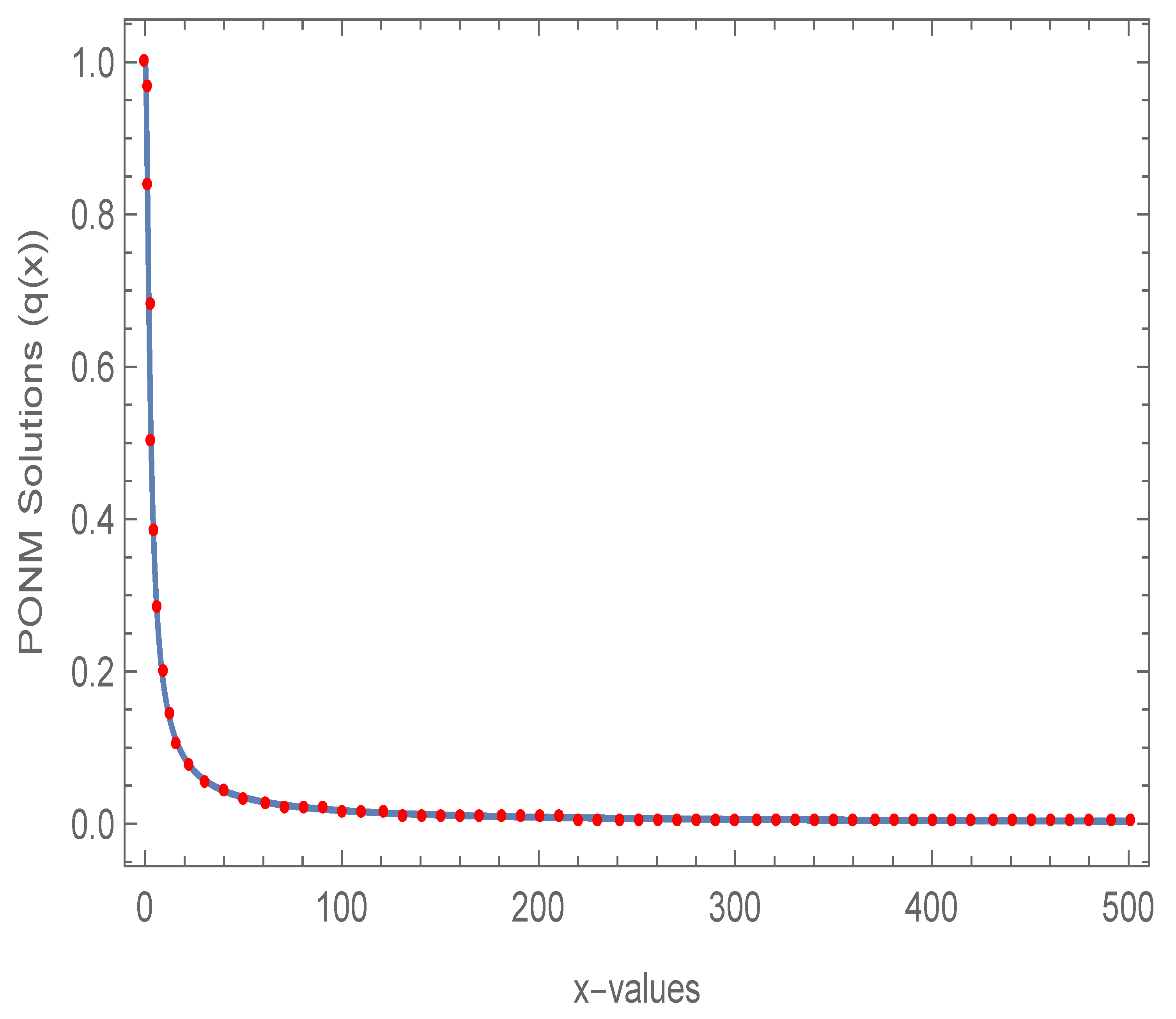
4.1. Problem One
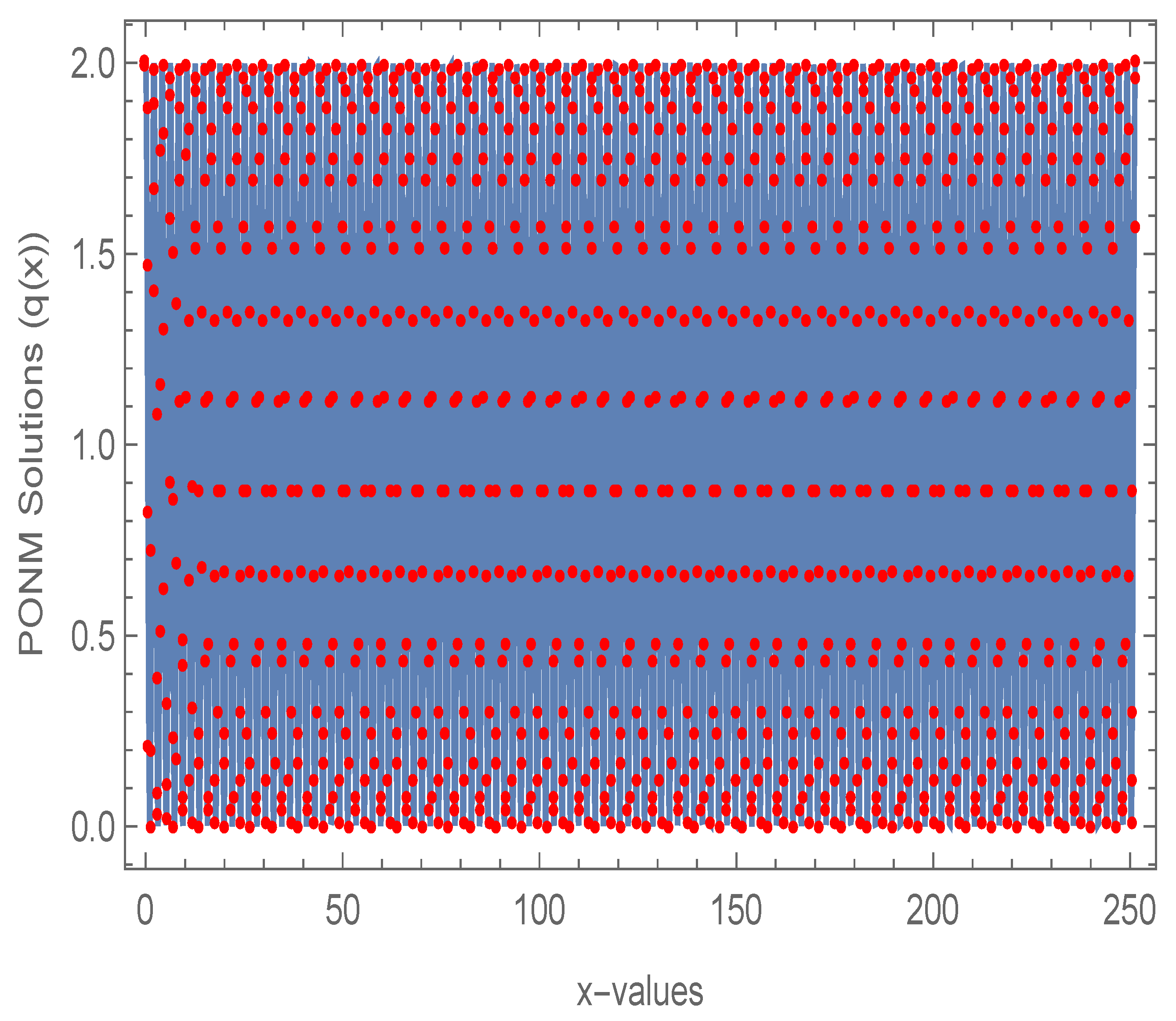
4.2. Problem Two
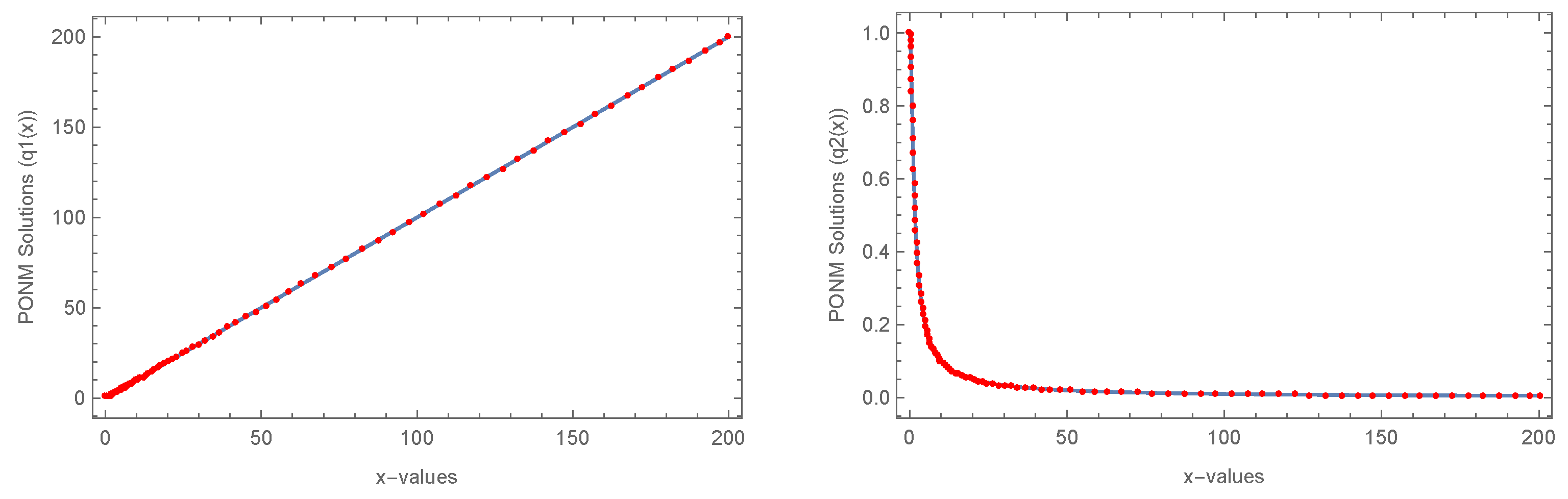
4.3. Problem Three
5. Conclusions
Author Contributions
Funding
Data Availability Statement
Conflicts of Interest
References
- Agarwal, R.P.; O’Regan, D. Second order initial value problems of Lane-Emden type. Appl. Math. Lett. 2007, 20, 1198–1205. [Google Scholar] [CrossRef] [Green Version]
- Biles, D.C.; Robinson, M.P.; Spraker, J.S. A generalization of the Lane-Emden equation. J. Math. Anal. Appl. 2002, 273, 654–666. [Google Scholar] [CrossRef]
- Chandrasekhar, S. Introduction to Study of Stellar Structure; Dover: New York, NY, USA, 1967. [Google Scholar]
- Rufai, M.A.; Ramos, H. Numerical integration of third-order singular boundary-value problems of Emden–Fowler type using hybrid block techniques. Commun. Nonlinear Sci. Numer. Simul. 2022, 105, 106069. [Google Scholar] [CrossRef]
- Rufai, M.A.; Ramos, H. Solving third-order Lane–Emden–Fowler equations using a variable step-size formulation of a pair of block methods. J. Comput. Appl. Math. 2023, 420, 114776. [Google Scholar] [CrossRef]
- Rufai, M.A.; Ramos, H. Numerical Solution for Singular Boundary Value Problems Using a Pair of Hybrid Nyström Techniques. Axioms 2021, 10, 202. [Google Scholar] [CrossRef]
- Shawagfeh, N.T. Nonperturbative approximate solution for Lane-Emden equation. J. Math. Phys. 1993, 34, 4364–4369. [Google Scholar] [CrossRef]
- Koch, O.; Kofler, P.; Weinmüller, E.B. The implicit Euler method for the numerical solution of singular initial value problems. Appl. Numer. Math. 2000, 34, 231–252. [Google Scholar] [CrossRef]
- Chowdhury, M.S.H.; Hashim, I. Solution of a class of singular second-order IVPs by homotopy-perturbation method. Phys. Lett. A 2007, 365, 439–447. [Google Scholar] [CrossRef]
- Mehrpouya, M.A. An efficient pseudospectral method for numerical solution of nonlinear singular initial and boundary value problems arising in astrophysics. Math. Methods Appl. Sci. 2016, 39, 3204–3214. [Google Scholar] [CrossRef]
- Bhrawy, A.H.; Alofi, A.S. A Jacobi-Gauss collocation method for solving nonlinear Lane-Emden type equations. Commun. Nonlinear Sci. Numer. Simul. 2012, 17, 62–70. [Google Scholar] [CrossRef]
- Swati; Singh, K.; Verma, A.K.; Singh, M. Higher order Emden–Fowler type equations via uniform Haar Wavelet resolution technique. J. Comput. Appl. Math. 2020, 376, 112836. [Google Scholar] [CrossRef]
- Sabir, Z.; Raja, M.A.Z.; Umar, M. Design of neuro-swarming-based heuristics to solve the third-order nonlinear multi-singular Emden–Fowler equation. Eur. Phys. J. Plus 2020, 135, 410. [Google Scholar] [CrossRef]
- Rufai, M.A.; Ramos, H. Numerical solution of second-order singular problems arising in astrophysics by combining a pair of one-step hybrid block Nyström methods. Astrophys. Space Sci. 2020, 365, 96. [Google Scholar] [CrossRef]
- Singh, R.; Kumar, J. The Adomian decomposition method with Green’s function for solving nonlinear singular boundary value problems. J. Appl. Math. Comput. 2014, 44, 397–416. [Google Scholar] [CrossRef]
- Rufai, M.A.; Ramos, H. A variable step-size fourth-derivative hybrid block strategy for integrating third-order IVPs, with applications. Int. J. Comput. Math. 2022, 99, 292–308. [Google Scholar] [CrossRef]
- Heydari, M.; Hosseini, S.M.; Loghmani, G.B. Numerical solution of singular IVPs of Lane-Emden type using integral operator and radial basis functions. Int. J. Ind. Math. 2012, 4, 135–146. [Google Scholar]
- Dong, Q.L. A new iterative method with alternated inertia for the split feasibility problem. J. Nonlinear Var. Anal. 2021, 5, 939–950. [Google Scholar]
- Zhang, J.; Shen, Y.; He, J. Some analytical methods for singular boundary value problem in a fractal space: A review. Appl. Comput. Math. 2019, 18, 225–235. [Google Scholar]
- Ascher, U.M.; Petzold, L.R. Computer Methods for Ordinary Differential Equations and Differential-Algebraic Equations; Society for Industrial and Applied Mathematics (SIAM): Philadelphia, PA, USA, 1998. [Google Scholar]
- Shampine, L.F.; Gordon, M.K. Computer Solutions of Ordinary Differential Equations: The Initial Value Problem; Freeman: San Francisco, CA, USA, 1975. [Google Scholar]
- Stoer, J.; Bulirsch, R. Introduction to Numerical Analysis; Springer: Berlin/Heidelberg, Germany, 2002. [Google Scholar]
- Yıldırım, A.; Özis, T. Solutions of singular IVPs of Lane-Emden type by homotopy perturbation method. Phys. Lett. A 2007, 369, 70–76. [Google Scholar] [CrossRef]
- Chawla, M.M.; Jain, M.K.; Subramanian, R. The application of explicit Nyström methods to singular second order differential equations. Comput. Math. Appl. 1990, 19, 47–51. [Google Scholar] [CrossRef] [Green Version]
- Rahimkhani, P.; Ordokhani, Y. Orthonormal Bernoulli wavelets neural network method and its application in astrophysics. Comp. Appl. Math. 2021, 40, 78. [Google Scholar] [CrossRef]
- Ramos, H.; Rufai, M.A. An adaptive pair of one-step hybrid block Nyström methods for singular initial-value problems of Lane–Emden–Fowler type. Math. Comput. Simul. 2022, 193, 497–508. [Google Scholar] [CrossRef]
- Wang, H.; Zhang, C. The adapted block boundary value methods for singular initial value problems. Calcolo 2018, 55, 22. [Google Scholar] [CrossRef]


| ABTOL | Method | NS | MAE |
|---|---|---|---|
| PONM | 3 | ||
| HPM | 4 | ||
| WNT | 4 | ||
| PONM | 4 | ||
| HPM | 5 | ||
| WNT | 5 |
| ABTOL | Method | NS | TFE | CPU | MAE |
|---|---|---|---|---|---|
| PONM | 57 | 284 | |||
| NM | 58 | 289 | |||
| NM | 61 | 304 | |||
| NM | 64 | 319 | |||
| PONM | 72 | 359 | |||
| NM | 80 | 399 |
| ABTOL | Method | NS | MAE |
|---|---|---|---|
| PONM | 22 | ||
| BVM | 40 | ||
| PONM | 43 | ||
| BVM | 80 | ||
| PONM | 88 | ||
| BVM | 160 |
| ABTOL | Method | NS | TFE | CPU | MAE |
|---|---|---|---|---|---|
| PONM | 397 | 1984 | |||
| NM | 577 | 2884 | |||
| PONM | 843 | 4214 | |||
| NM | 1209 | 6044 | |||
| PONM | 1772 | 8859 | |||
| NM | 2541 | 12704 |
| ABTOL | Method | NS | FE | CPU | MAE |
|---|---|---|---|---|---|
| PONM | 40 | 199 | |||
| NM | 43 | 214 | |||
| PONM | 55 | 274 | |||
| NM | 59 | 294 | |||
| PONM | 78 | 389 | |||
| NM | 82 | 409 |
Disclaimer/Publisher’s Note: The statements, opinions and data contained in all publications are solely those of the individual author(s) and contributor(s) and not of MDPI and/or the editor(s). MDPI and/or the editor(s) disclaim responsibility for any injury to people or property resulting from any ideas, methods, instructions or products referred to in the content. |
© 2023 by the authors. Licensee MDPI, Basel, Switzerland. This article is an open access article distributed under the terms and conditions of the Creative Commons Attribution (CC BY) license (https://creativecommons.org/licenses/by/4.0/).
Share and Cite
Rufai, M.A.; Ramos, H. Solving SIVPs of Lane–Emden–Fowler Type Using a Pair of Optimized Nyström Methods with a Variable Step Size. Mathematics 2023, 11, 1535. https://doi.org/10.3390/math11061535
Rufai MA, Ramos H. Solving SIVPs of Lane–Emden–Fowler Type Using a Pair of Optimized Nyström Methods with a Variable Step Size. Mathematics. 2023; 11(6):1535. https://doi.org/10.3390/math11061535
Chicago/Turabian StyleRufai, Mufutau Ajani, and Higinio Ramos. 2023. "Solving SIVPs of Lane–Emden–Fowler Type Using a Pair of Optimized Nyström Methods with a Variable Step Size" Mathematics 11, no. 6: 1535. https://doi.org/10.3390/math11061535