Impact of Geopolitical Risk on G7 Financial Markets: A Comparative Wavelet Analysis between 2014 and 2022

Abstract

This study investigates co-movements between the GPR generated by the Crimean Peninsula’s annexation in 2014, the Russia–Ukraine war in 2022, and the volatility of stock markets in the G7 states. Using wavelet analysis, concentrated co-movement was found for all indices in both periods. Contrary to the general perception, we find that the G7 financial market response in 2014 was robust. Using a time-varying parameter vector autoregression (TVP-VAR) test, we found a larger reaction in the amplitude of the G7 financial markets in 2022 than in 2014. The financial markets in France, Germany, and the UK showed a similar reaction in 2022. We have identified some common aspects, even if the political and military contexts of the two studied events were completely different. Our findings offer new and interesting implications for understanding how geopolitical risk affects financial assets for market participants with multiple investment horizons and strategies.

1. Introduction

The geopolitical events that took place after WW2 constituted factors of uncertainty regarding local or global action. Geopolitical risks (GPRs) involve acts of terrorism, tensions between regions or states, nuclear threats, terrorism, and war, all of which affect the peace process in international relations [1]. GPRs influence national and international economies and financial markets, as they are exogenous factors that affect their equilibrium. The mode of transmission of shocks from the GPR to the main financial markets is being resolved [2].

The state of uncertainty caused by GPR causes investors to adjust their investment strategies in financial markets. Consequently, the participants were attentive to the influence of GPR on financial asset prices. For investors, tracking the impact of GPR contributes to investment decisions. For authorities, designing appropriate policies is beneficial for reducing volatility and strengthening market stability and balance. Stock return predictability has profound effects on financial and monetary policymaking, investment decisions, and risk management [3].

In general, financial markets are negatively impacted by significant GPR, as they lower stock prices and cause higher return volatility [4]. As stocks are affected by GPR, investors look to adjust their portfolios; consequently, there will be fewer riskier investments which will exacerbate the volatility of financial markets and further large price swings [5]. As a result, the time–frequency field’s interactions between GPR and stock market volatility allow the identification of potential heterogeneity resulting from the diversity of investment decisions [6].

The literature related to the Russia–Ukraine dispute is dominated by the different sanctions imposed on each other by the US, the EU, and Russia [6,7,8]. Military and political tensions affect large equity markets but can also cause abrupt shifts in risk exposure. However, there has been no comparative study of markets’ reactions to the two Ukraine-related GPR events. Furthermore, the difference in amplitude between the market reactions in 2014 and 2022 is unknown.

Based on previous findings and the objective of this research, we compare and analyze the link between GPR and stock volatility in the G7 states to fill a gap in the literature. Therefore, this research examines whether GPRs impacted stock markets during these two events and provides solutions to mitigate their effects in the future. Methodologically, wavelet analysis was used to characterize the relation between the GPRs and G7 markets. A frequency-based approach allows a global view of developed markets and is useful for all stock market participants as they make decisions within different timeframes.

Previous research has demonstrated that GPR influences asset prices through various pathways. Thus, economic announcements [9], political events or tensions [10], event-related news [11], acts of terrorism [12], and supply disruption [13] can influence the uncertainty (risk) of assets. The greatest weight is given to the news in the research carried out on the segments of the stock markets, taking into account different time periods. For example, Chen and Li (2023) demonstrated that fundamental and nonfundamental news generated volatility of different intensity and magnitude even if scheduled or unscheduled [14]. Moreover, the asset price is affected with different intensities during the events or after their development [15]. Geopolitical risks can remain net transmitters of shock, but they turned into net receivers of shock over a period [16].

The main contributions of this study are as follows: First, we propose a common approach to GPR and volatility in the G7 states to research how they affect returns on financial assets. Second, an analysis was performed to compare the time–frequency influence of GPR. Finally, it provides a comprehensive understanding of the inhomogeneous responses to the shocks induced by these two military events. Given that stock volatility and returns are fundamental indicators for stock market participants, their predictability is important in guiding portfolio management [17,18]. Our results complement the literature by considering nonlinear models that demonstrate predictability within a particular timeframe and frequency.

The remainder of this article is organized as follows: Section 2 provides a summary of the literature, Section 3 organizes the data and discusses the methodology, Section 4 describes the findings, Section 5 includes discussions, Section 6 contains robustness tests, and Section 7 offers a set of conclusions.

2. Literature

With the escalation of the conflict in Ukraine, political and military risks have attracted the interest of researchers, as the uncertainties related to armed conflict have attracted both attention and fear. The literature presents a link between GPR and the uncertain state of financial markets. Recent models commonly used for this purpose include the economic policy uncertainty index (EPU) [19], the financial stress index (NFSI) [20], and the volatility index (VIX) [21,22].

The escalation of the war caused problems in the global supply chain, imbalances in raw materials and energy markets, financial and economic sanctions applied by both sides or other neutral states, and events reflected in financial markets. Studies on stocks published after the outbreak of conflict in Ukraine, such as [23,24], show a strong correlation between war and financial assets. Zhang et al. (2022) claimed that the war broke out as the largest military event since World War II, and at the end of February 2022, financial markets in Europe and the US experienced a negative shock [6]. Lo et al. (2022) considered 73 countries to evaluate the influence of the Russia–Ukraine war on stock markets [25]. The authors presented evidence that financial markets reacted considerably to war-induced risks and that volatility was higher than asset price dynamics. Sun and Zhang (2022) conducted a comprehensive analysis of a sample of 86 states. The authors analyzed the influence of heterogeneous factors on returns around the date of the war outbreak [26].

Research focusing on regional markets or companies after the war has revealed negative aspects. Bougias et al. (2022) conclude that the war caused greater volatility in assets and corporate security in European companies [27]. After the escalation of the dispute between Ukraine and Russia in 2022, Fang and Shao (2022) demonstrated increased volatility in the agricultural, energy, and extractive markets [28]. According to Singh et al. (2022) the Russia–Ukraine military conflict caused a migration of investors’ priorities to the energy, aerospace, and defense sectors [29]. Umar et al. (2022) demonstrated an increase in abnormal returns in Europe on the pricing of metals and energy [30].

The literature review includes comparative analyses conducted before and after 24 February 2022. Adekoya et al. (2023) found a link between high stock market and oil market prices before and during the conflict [31]. Yousaf et al. (2022) compiled a study of financial markets in the G20 countries. The authors presented evidence that most states experienced abnormally negative shocks before and during the days after the start of the war, particularly on the Russian market [32]. Another comparative study was conducted by Ha (2023) to examine the volatility of financial markets from January 2018 to April 2022. The author demonstrated that the war waves impacted global connection and that the gold and oil markets played the role of transmitters [33]. Using quantile regression, Bossman and Gubareva (2023) analyzed the impact of GPR on the G7 and E7 states. Based on an analysis period between 24 February 2022 and 25 July 2022, the authors established that the impact is asymmetric and specific to each analyzed state [34].

GPR is another fundamental factor influencing financial markets, as it provides incremental explanations for uncertainty in economic policy, financial stress, and volatility [3]. He (2023) pointed out that GPR can significantly influence trading decisions and investor sentiment [35]. Abbassi et al. (2022) concluded that stock prices depend considerably on trade and are fragile to GPR [36]. Shaik et al. (2023) showed that GPR affected stock, gold, and oil returns during the disruptive events of the worldwide economic downturn, COVID-19, and the 2022 Russia–Ukraine war [37]. Salisu et al. (2023) emphasized the predictive value of GPR in the global financial cycle (GFCy) [38]. Li et al. (2023) found that GPR affects the cost of natural resources, which are necessary for a healthy economy and way of life [39]. Agyei (2023) investigated the asymmetric relationship between stock markets and the GPRs of seven leading emerging economies in a dispute between Russia and Ukraine. The author emphasized that the emerging countries analyzed were suitable for diversifying and hedging portfolios against GPR risk [40]. Elsayed and Helmi (2021) demonstrated the main role of GPR in the transmission of volatility and spread dynamics in financial markets [41]. Several researchers have demonstrated the significance of crude oil returns and GPR on stock prices from a dynamic perspective [42,43,44,45].

The integration of stock markets in developed countries through the correlation between volatility and returns has been demonstrated over time. US markets play a key role in managing uncertainty in global financial markets. Uncertainty is rife across the globe, as heightened volatility in US markets spills over to global markets [46]. The G7 capital markets are representative because they have high levels of development, regulation, supervision, good capitalization, and liquidity [46,47].

The phenomenon that denotes the transmission of shocks to other countries due to some generating factors is called the “contagion effect”. Although there is no consensus on the causes that determine the occurrence of this phenomenon [48], research demonstrates that extreme events can cause shocks that are transmitted between stock markets [49]. Such shocks are caused by the increasingly intense links between stock markets and are transmitted from large markets to neighboring ones through different channels and to smaller markets. This phenomenon was accentuated during the COVID-19 pandemic [50,51,52] and during the war in Ukraine [53].

Currently, the connection between the two analyzed events is unclear. The annexation of the Crimean Peninsula on 21 March 2014 escaped the attention of researchers, and the financial literature on this subject is quite limited. Research related to the annexation of the Crimean Peninsula has dealt with various aspects of this conflict, including military, political, social, and economic aspects. Some authors have focused on legitimacy, public opinion, human rights violations, and crimes against humanity [54,55]. Few studies on the economic influence of the Crimean crisis have focused on the economic impact of reciprocal sanctions, trade or tariff barriers, limited access to EU capital markets, travel visa rejections, asset freezes of individuals or companies, and the withdrawal of large European or North American companies [56,57,58,59,60]. It is estimated that the annexation of the Crimean Peninsula generated less volatility in the main markets, but its amplitude is not known. In addition, the fact that there are two connected events was not considered.

Although they arouse fear and uncertainty, relatively few studies have been conducted on the influence of military conflicts on financial markets before the start of the conflict in Ukraine in 2022. Furthermore, due to the lack of literature and volatility estimations, there is no agreement on the response of financial markets to wars. Therefore, a time–frequency model is used to analyze and compare time-varying stock returns. This study is an early exploration of the integration of two military events in Ukraine to study their effects on volatility and stock returns.

3. Data and Methodology

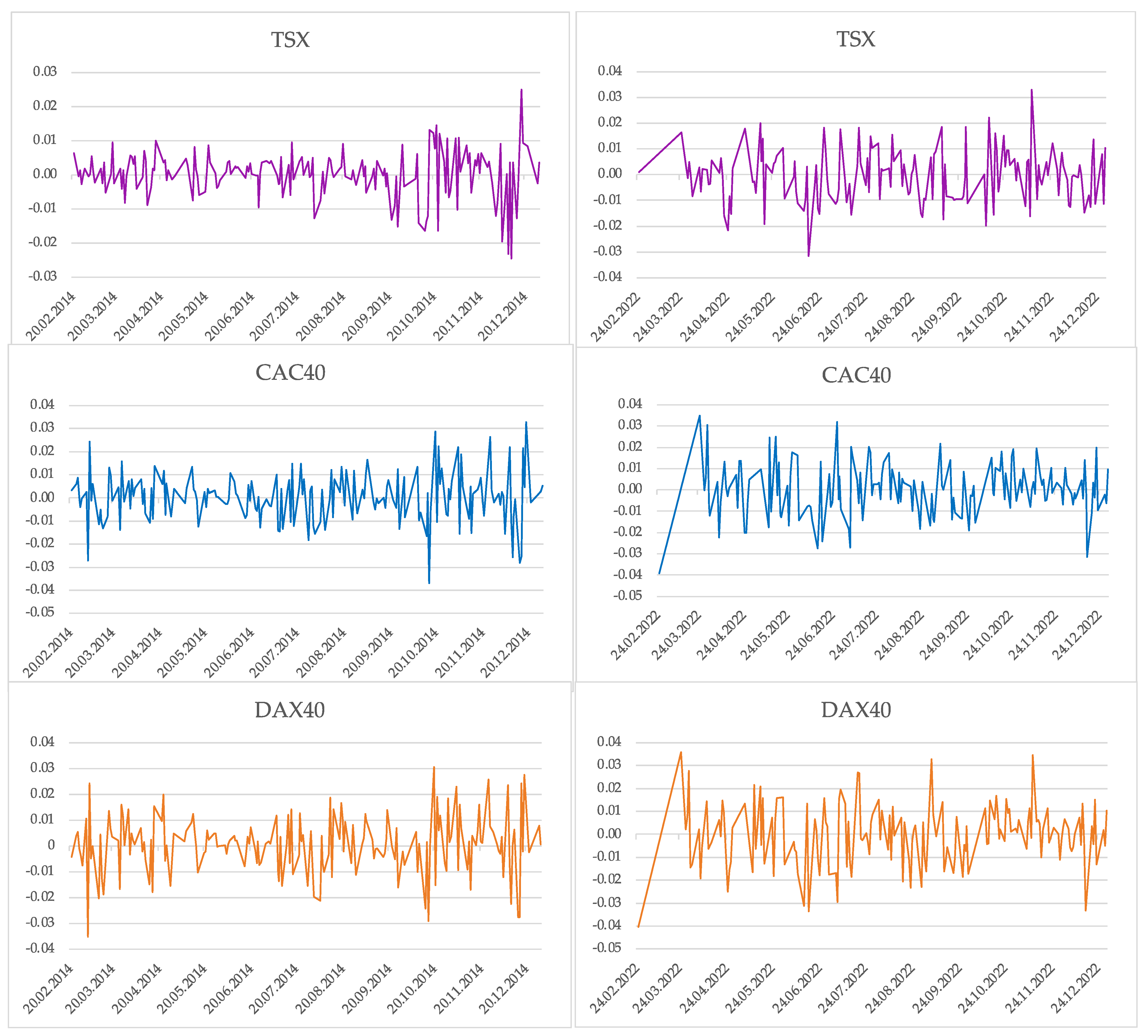
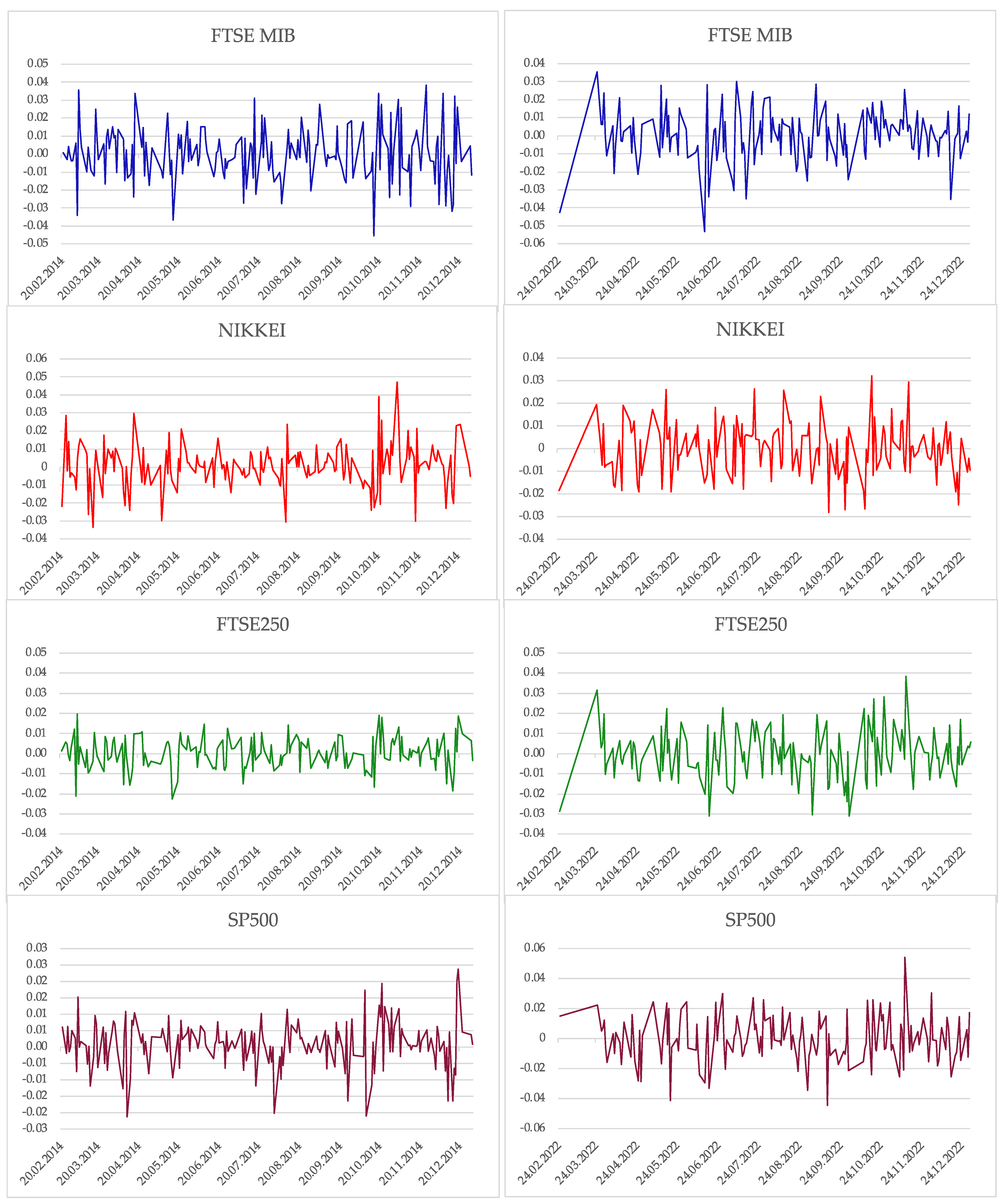
3.1. Data and Sources

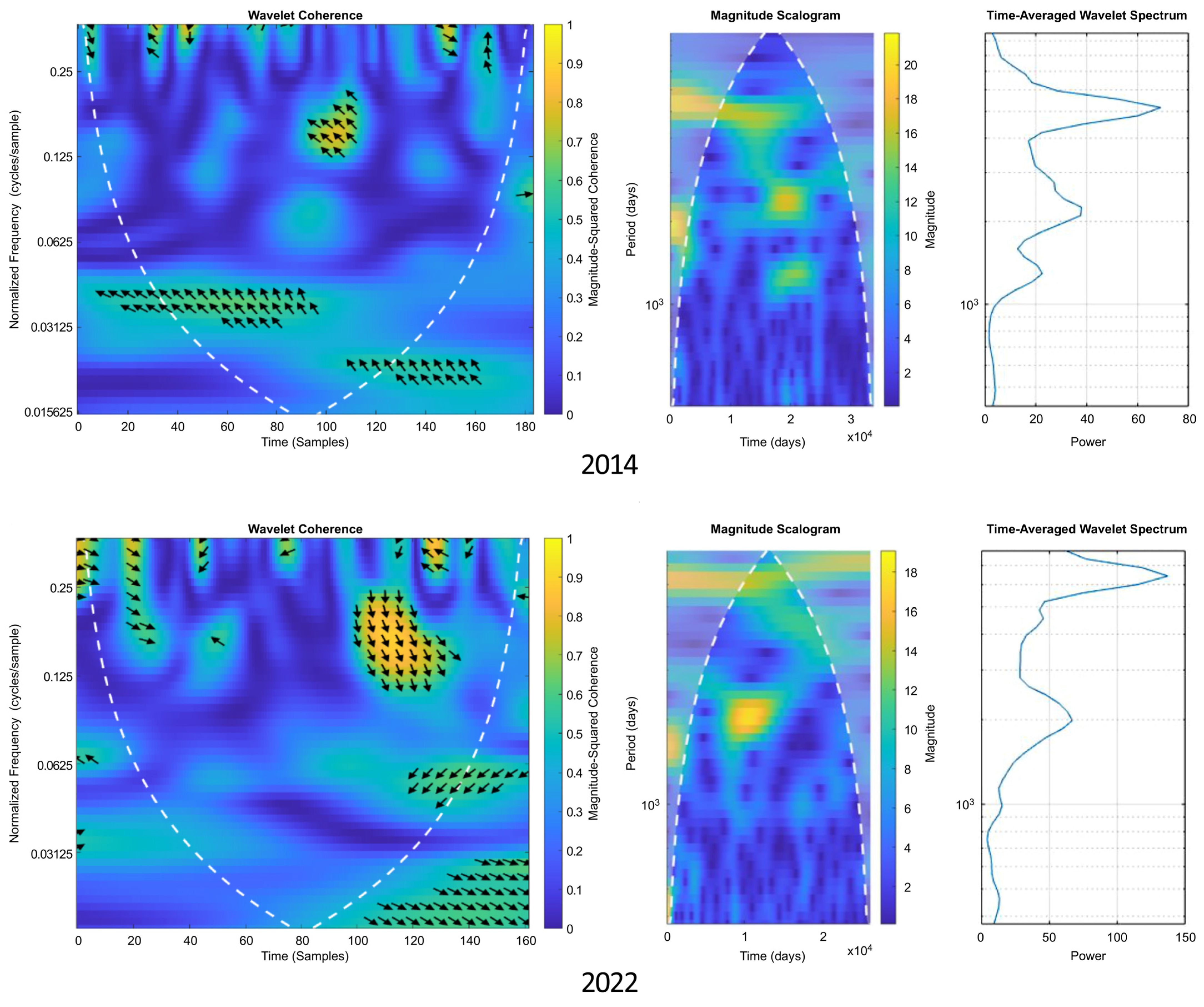
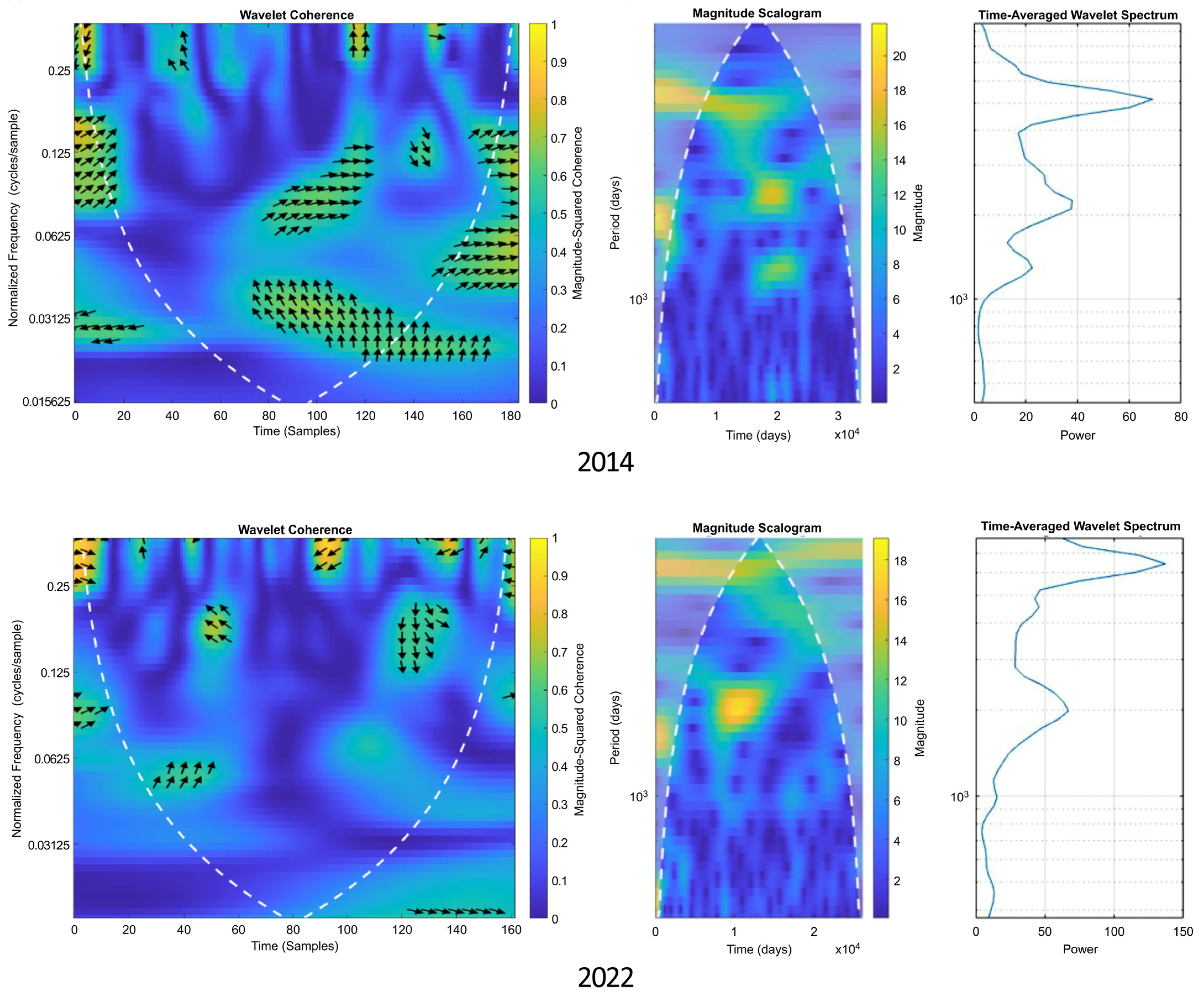
This study investigates the interactions between the GPR generated by the Crimean Peninsula’s annexation in 2014, the Russia–Ukraine war in 2022, and the volatility of stock markets in the G7 states (Canada, France, Germany, Italy, Japan, the UK, and the US). For the annexation of the Crimean Peninsula, the analyzed period is between 20 February 2014 and 31 December 2014, and to capture the Russia–Ukraine war, the analysis period is between 24 February 2022 and 31 December 2022. The week of five trading days is used for all analyzed states. Daily data were collected on representative stock indices (TSX, CAC40, DAX40, FTSE MIB, NIKKEI, FTSE250, and SP500) from the www.stook.com platform and daily returns were determined. Daily GPR index data were collected using the platform https://www.matteoiacoviello.com/gpr.htm, accessed on 23 July 2023. The first logarithmic difference between the daily closing prices was calculated using Equation (1):

$$R_{i,t}={\ln (P}_{i,t})-{\ln (P}_{i,t-1,}),$$

(1)

where ln is the natural logarithm; P_i,t−1 is the price of the stock in period t − 1; P_i,t is the price of stock i in period t; and R_i,t is the yield of stock i in period t [32,40,61].

Table 1. Series statistics for G7 stock returns in 2014.

Index	TSX	CAC40	DAX40	FTSE MIB	NIKKEI	FTSE250	SP500
Mean	0.0004	0.0002	0.0004	−0.7471	0.0008	−0.0004	0.0009
Median	0.0008	0.0006	0.0010	0.4600	0.0009	−0.0003	0.0009
Maximum	0.0251	0.0329	0.0307	27.1400	0.0471	0.0356	0.0237
Minimum	−0.0244	−0.0370	−0.0350	−33.6900	−0.0335	−0.0454	−0.0211
Std. dev.	0.0067	0.0106	0.0110	9.6257	0.0122	0.0150	0.0070
Skewness	−0.6226	−0.0893	−0.1880	−0.2699	0.1272	0.0353	−0.2726
Kurtosis	5.1890	4.0446	3.7125	3.3475	4.5860	3.1579	4.5179

Notes: The sample’s statistical characteristics are shown in this table. The returns on G7 stock markets are included in the sample. The series period starts from 20 February 2014 to 31 December 2014.

and

Table 2. Series statistics for G7 stock returns in 2022.

Index	TSX	CAC40	DAX40	FTSE MIB	NIKKEI	FTSE250	SP500
Mean	−0.0006	−0.0002	−0.0005	−0.0002	−0.0005	−0.0004	−0.0003
Median	−0.0002	−0.0010	0.0002	0.0003	0.0003	−0.0011	−0.0016
Maximum	0.0329	0.0349	0.0360	0.0353	0.0320	0.0383	0.0540
Minimum	−0.0315	−0.0390	−0.0404	−0.0531	−0.0282	−0.0311	−0.0442
Std. dev.	0.0101	0.0124	0.0134	0.0142	0.0115	0.0125	0.0153
Skewness	0.1556	0.0296	−0.0802	−0.4236	0.1148	0.1556	0.0928
Kurtosis	3.1845	3.3959	3.3583	4.0241	3.0455	3.1452	3.5733

Notes: The sample’s statistical characteristics are shown in this table. The returns on G7 stock markets are included in the sample. The series period starts from 24 February 2022 to 31 December 2022.

contain the descriptive statistics for the two analyzed periods, and plots of stock returns from the G7 states are shown in Figure 1. Statistical data were processed with EViews 13 software (Quantitative Micro Software, Irvine, CA, USA) and MATLAB version 9.13.0 (R2022b).

3.2. Methodology

A wavelet (or ondelette), notated ψ$\left(t\right)\in L^2\left(R\right)$, is a square-integrable continuous function with a real or complex value, usually called the mother wavelet, which satisfies some constraints as ${\int }_{-\infty }^{\infty }\psi (t)\mathrm{dt}=0$ and ${\int }_{-\infty }^{\infty }{\left|\psi \left(t\right)\right|}^2\mathrm{dt}<\infty$ [6,37,40,62,63,64,65,66,67,68,69,70,71,72]. Starting from the mother wavelet ψ(t), the daughter wavelet family ${\psi }_{\tau ,s}\left(t\right)$ is obtained through scaling and translation operations on the time axis. The variable τ ensures the displacement of the function on the time axis $\psi \left(\tau \right)=\psi (t-\tau )$, and s allows the matching of the wavelet function with the transformed time series ψ$\left(s\right)=\psi \left(\frac{t}{s}\right).$ A continuous Morlet-type wavelet was used, consistent with Daubechies [68] and Mallat [69], and is defined in Equation (2) as follows:

$${\psi }^M\left(t\right)={\pi }^{-\frac{1}{4}}{·e}^{i{\omega }_{0}t}·e^{-\frac{t^2}{2}},$$

(2)

where i is the imaginary part of the wavelet function centered at the point (0, ω₀/2π), and ω₀ represents the center frequency of the wavelet. The relationship between the frequency and scale defined in Equation (3) is:

$$f=\frac{{\mu }_f}{s}\approx \frac{1}{s}.$$

(3)

Equations (4) and (5) can be used to estimate the wavelet transformation of x(t) and y(t) as follows:

$$W_{x:\psi }\left(\tau ,s\right)={\int }_{-\infty }^{\infty }x\left(t\right)\frac{1}{\sqrt{⌊s⌋}}{\mathsf{\Psi }}^{*}\left(\frac{t-\tau }{s}\right)\mathrm{dt},$$

(4)

$$W_{y:\psi }\left(\tau ,s\right)={\int }_{-\infty }^{\infty }y\left(t\right)\frac{1}{\sqrt{⌊s⌋}}{\mathsf{\Psi }}^{*}\left(\frac{t-\tau }{s}\right)\mathrm{dt}.$$

(5)

The wavelet power spectrum (WPS), which measures the degree of volatility across time dimensions, can be created after transforming x(t) and y(t) using the prior in relation to (6).

$${\mathit{WPS}}_{x\left(y\right)}={\left[W_{x\left(y\right)}\left(\tau ,s\right)\right]}^2.$$

(6)

The magnitude and time-averaged wavelet spectra are two instruments that can be used to extend the WPS to a bivariate function. Time series x(t) and y(t) have the following wavelet coherence, expressed by Torrence and Webster (1999) [73] in Equation (7) [67]:

$$R_{x,y}^2\left(\tau ,s\right)=\frac{{\left|S\left(s^{-1}{W}_{x_i{y}_j}\left(\tau ,s\right)\right)\right|}^2}{S\left(s^{-1}{\left|W_{x_i}\left(\tau ,s\right)\right|}^2\right)\times S\left(s^{-1}{\left|W_{x_j}\left(\tau ,s\right)\right|}^2\right)},$$

(7)

where $R^2\in \left[0,1\right]$, $W_{x_i{x}_j}$ is the wavelet cross spectrum (WCS) between x(t) and y(t), W_xi and W_yj are the wavelet transformations of x(t) and y(t), s is the parameter of scale, τ is the parameter of location, and S is the smooth operator.

4. Results

For each G7 state, two paired time series are formed, consisting of the values for the GPR index and the volatility of each stock index. Figure 2, Figure 3, Figure 4, Figure 5, Figure 6, Figure 7 and Figure 8 show a contour map for each analyzed state containing the wavelet coherence, magnitude scalogram, and time-averaged wavelet spectrum. Such a graphical representation is frequently encountered in the economic literature [70,71,72]. The associated colors in the figures show the strength of the phase difference, varying from low intensity (blue) to maximum intensity (yellow). The yellow areas show high coherence between the pairs of variables, whereas the blue areas have the opposite meaning.

Figure 2, Figure 3, Figure 4, Figure 5, Figure 6, Figure 7 and Figure 8 show eight one-way arrows, a cone of influence (COI), and two axes (left side of each figure). The Ox axis includes the analyzed period, and the Oy the normalized frequency in the form of a coefficient between zero and one. The phase difference analysis is represented by the direction of the arrows in the scalogram. If the arrows point to the right, the time series are positively correlated, and if the arrows point to the left, the correlation is negative. Arrows pointing right and up (↗) or left and down (↙) highlight that the first variable (GPR) has the primary role. Arrows oriented to the left and up (↖) or the right and down (↘) indicate a leading role for the second variable (stock returns). The ↑ and (↓) arrows show that GPR leads stock return with π/2. The COI describes the significant dynamics of the interaction between the analyzed pairs with a dashed white line. Thus, positioning within the COI shows significant dynamics, and outside the COI is a faded area indicating insignificant dynamics. The pairs of time series shifted together on a certain time scale according to a zero-phase difference [74].

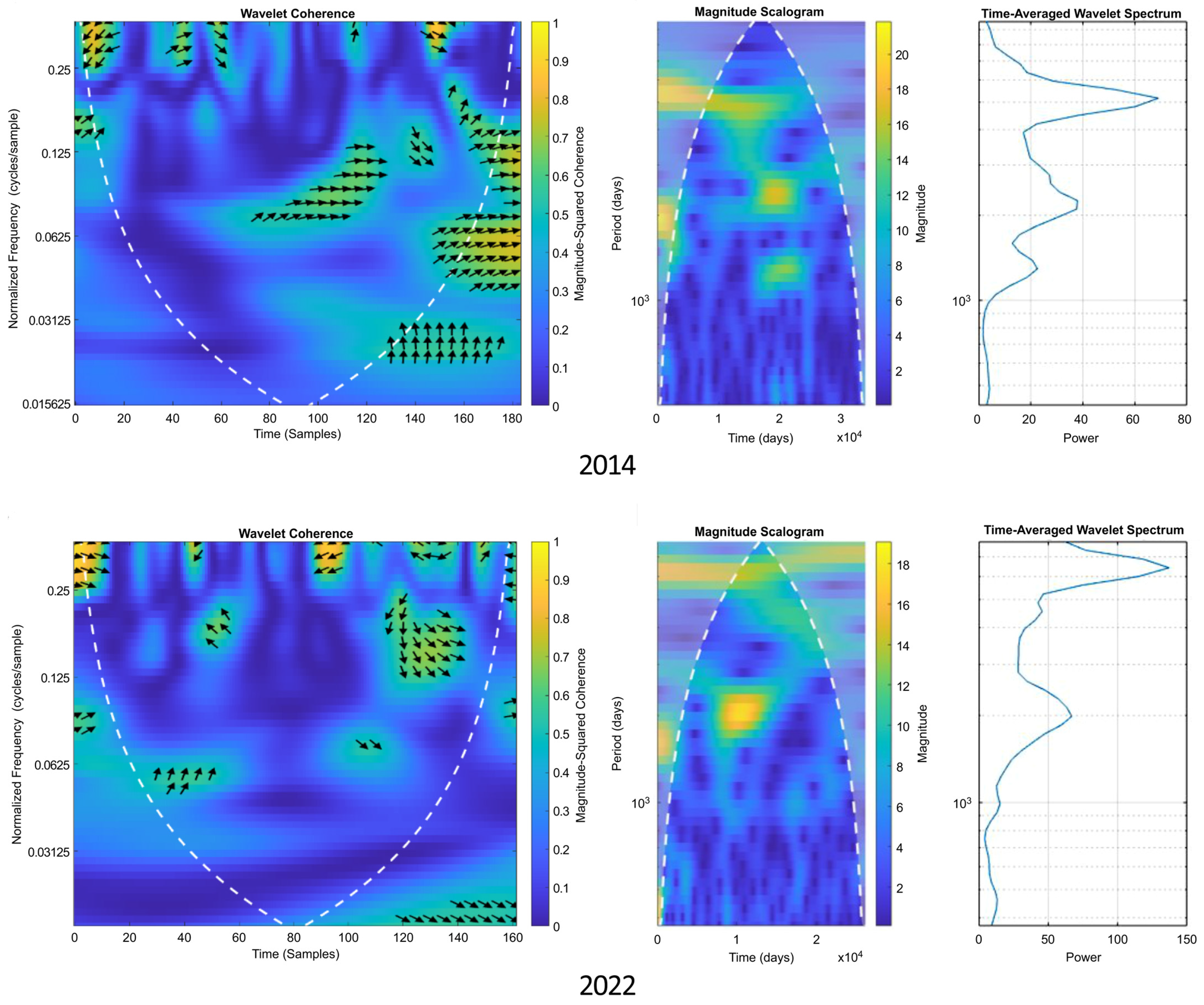
4.1. Comparative Analysis between GPR and Canada Stocks in 2014 and 2022

Figure 2 shows the dynamics of the correlation between GPR and Canadian stock returns. A medium level of consistency was observed for both 2014 and 2022. The heat map was mostly blue in 2014, with a few clouds of arrows pointing to the left and up. The most consistent cloud of arrows was found in the first 80 days after the annexation of the Crimean Peninsula. During Ukraine’s invasion in 2022, the commotion was more pronounced than it was in 2014, which means that Canadian financial markets responded more strongly to military conflict. Arrows point to the left and right in the range of normalized frequencies between 0.03125 and 0.0625, indicating a slight negative correlation. In 2022, the co-movement is significant in the low-frequency band, with the arrows pointing to the right and down.

Figure 2. Geopolitical risk index and stock returns in Canada in 2014 and 2022.

Figure 2. Geopolitical risk index and stock returns in Canada in 2014 and 2022.

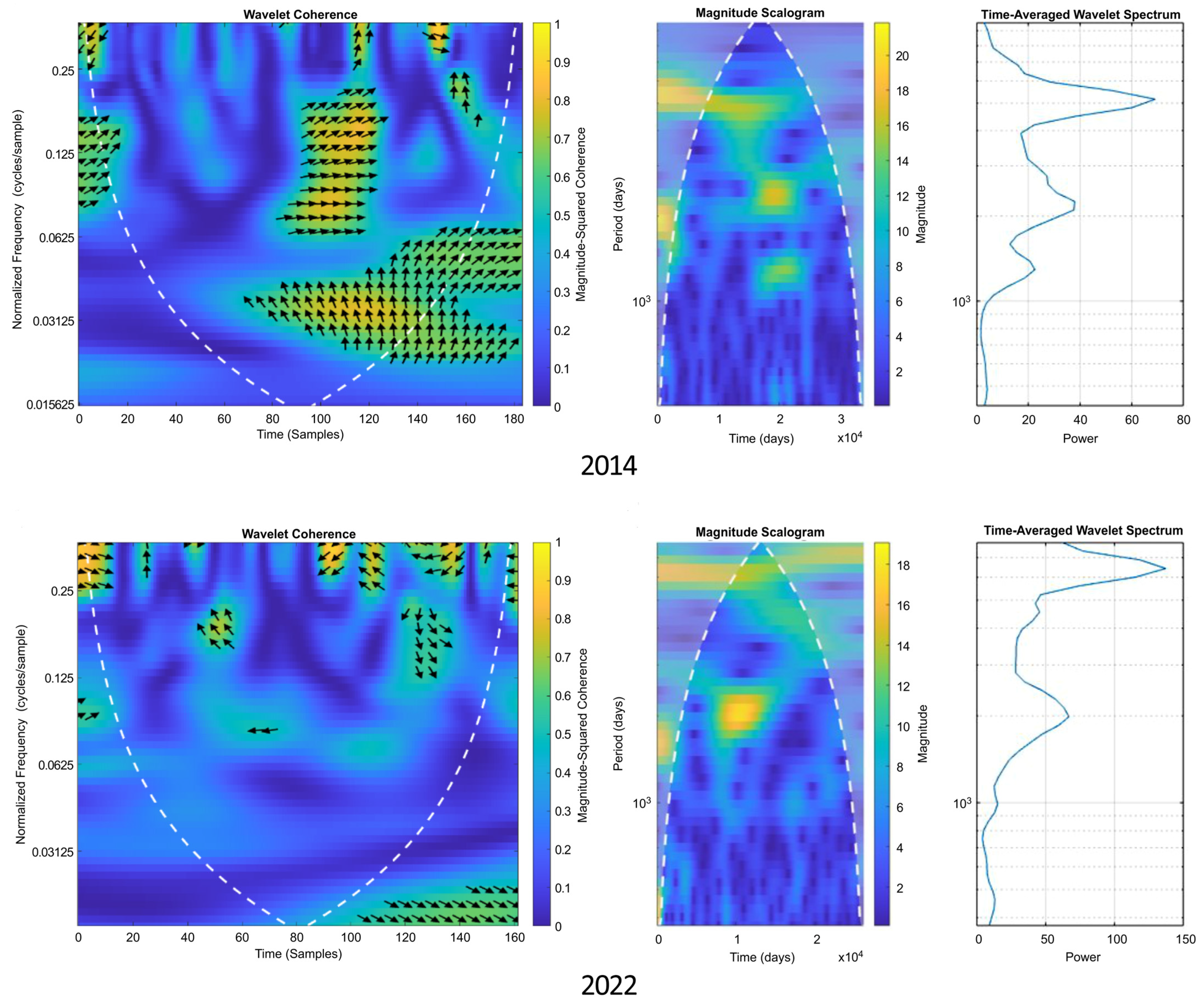
4.2. Comparative Analysis between GPR and France Stocks in 2014 and 2022

Figure 3 compares the trade-offs between GPR dynamics and French stock returns. The results show a similar reaction in French markets in both periods. The scalogram is mostly blue in terms of average coherence for both 2014 and 2022. This was noticeable in the first few days after the annexation of the Crimean Peninsula and was less pronounced immediately after the start of the war in 2022. In 2014, the arrows on the bands of normalized frequencies between 0.03125 and 0.125 were oriented horizontally and positively correlated; in 2022, a less pronounced negative correlation was found. These conclusions were confirmed by the blue color of the COI. Although stronger commotion was observed in 2014, its intensity was lower, as can be seen in the time-averaged power spectrum (right column).

Figure 3. Geopolitical risk index and stock returns in France in 2014 and 2022.

Figure 3. Geopolitical risk index and stock returns in France in 2014 and 2022.

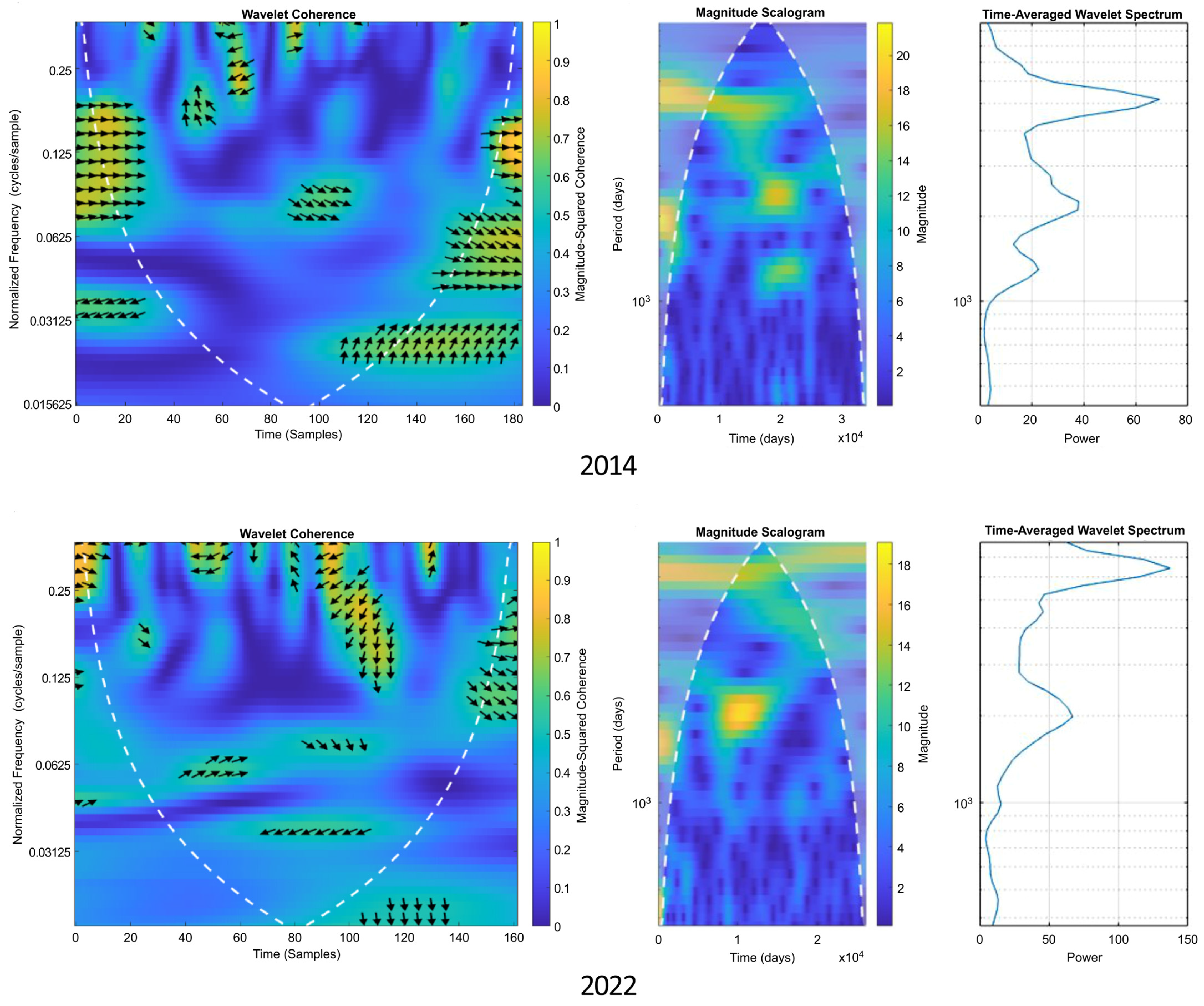
4.3. Comparative Analysis between GPR and Germany Stocks in 2014 and 2022

Figure 4 shows the dynamics of the GPR co-movements and stock returns in Germany. The results show the average levels of coherence in 2014 and 2022. If the heat map is colored blue in the lower-left part, in 2022 the map is predominantly colored blue. In 2014, a predominantly positive average coherence was found in all frequency bands, indicating that German stock returns are positively determined by GPR shocks. During the Ukrainian invasion in 2022, the situation changed significantly, as coherence was weaker and negative. Although more pronounced commotion can be found in 2014, its intensity is much lower than that in 2022. In addition, a similar dynamic of the markets in France, Germany, and the UK can be found in 2022.

Figure 4. Geopolitical risk index and stock returns in Germany in 2014 and 2022.

Figure 4. Geopolitical risk index and stock returns in Germany in 2014 and 2022.

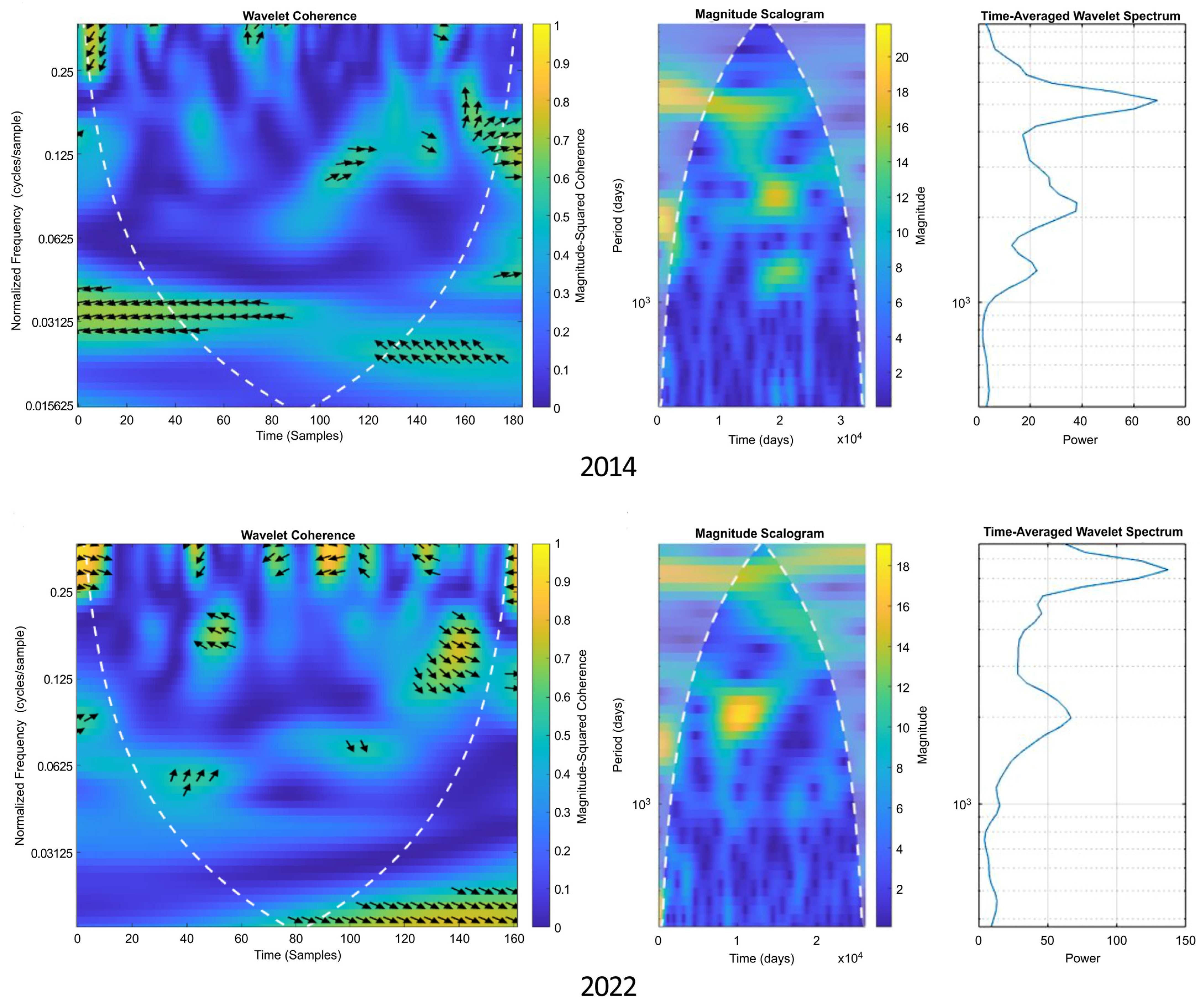
4.4. Comparative Analysis between GPR and Italy Stocks in 2014 and 2022

Figure 5 shows the dynamics of the GPR co-movements and stock returns in Italy. Similar to other G7 stock markets, the heat map is colored blue in the lower left, with all other areas showing high coherence in 2014. In the (80–180) day range, coherence was particularly high in the bands of average normalized frequency, suggesting that during the annexation of the Crimean Peninsula, Italian stock markets experienced some significant stress. In 2022, the scalogram is dominated by blue, which means a lower frequency of war on Italian shares, but of greater intensity. In the first few days after the beginning of the war, a negative commission manifested, and the arrows were oriented to the left in the band of normalized frequencies greater than 0.25.

Figure 5. Geopolitical risk index and stock returns in Italy in 2014 and 2022.

Figure 5. Geopolitical risk index and stock returns in Italy in 2014 and 2022.

4.5. Comparative Analysis between GPR and Japan Stocks in 2014 and 2022

Figure 6 shows the dynamics of GPR and stock returns in Japan. Environmental coherence is observed for both 2014 and 2022. In the lower left panel, a blue color appeared in 2014. In the first 30 days after the official annexation of Crimea in 2014, the Japanese market reacted negatively. In addition, significant reactions were found in the range of (120–200) days in the same year. In 2022, the commotions were average but of much higher intensity. The reaction of the Japanese markets to the normalized frequency band greater than 0.25 is strong and mainly negative.

Figure 6. Geopolitical risk index and stock returns in Japan in 2014 and 2022.

Figure 6. Geopolitical risk index and stock returns in Japan in 2014 and 2022.

4.6. Comparative Analysis between GPR and UK Stocks in 2014 and 2022

Figure 7 shows the dynamics between the GPR and UK equity returns. An average level of coherence was found for both analyzed periods. The heat map is dominated by the dark blue color in both periods. In 2014, the cloud of arrows pointing to the right or up observed in the normalized frequency band between 0.0625 and 0.125 indicates average negative commotions. In 2022, co-movements are more significant and differentiated. The days since the beginning of the Russia–Ukraine war brought a slight negative commotion in the normalized frequency band between 0.0625 and 0.125. The greater intensity with which the UK market reacts in 2022 compared to 2014 is visible in the right-hand column. An evolution similar to that of markets in France, Germany, and the UK is noteworthy, and is an aspect that explains the degree of integration of the largest financial markets in Europe in accordance with Liu et al. (2022) [3].

Figure 7. Geopolitical risk index and stock returns in UK in 2014 and 2022.

Figure 7. Geopolitical risk index and stock returns in UK in 2014 and 2022.

4.7. Comparative Analysis between GPR and US Stocks in 2014 and 2022

Figure 8 shows the dynamics of the trade-offs between GPR and US stock returns. In the US, medium and high levels were found in 2014 and 2022, respectively. The heat map is predominantly blue for 2014. In 2022, a permanent reaction of US stocks is found in the lowest frequency band. If, in 2014, the arrows are oriented differently on the frequency bands, showing an oscillating evolution, in 2022 the arrows are oriented to the right, horizontally, showing a positive commiseration of the stocks. In the band with the highest frequency, the impact of sanctions was not as pronounced as in the case of other G7 states, an aspect also reported by Wu et al. (2023) [46]. The reaction of actions immediately after the start of the military conflict was dominated by GPR, as the arrows were orientated toward the right, up from the normalized frequency band between 0 and 0.0625.

The comparative analysis between the co-movements identified in 2014 and 2022 based on Figure 2, Figure 3, Figure 4, Figure 5, Figure 6, Figure 7 and Figure 8 documents important aspects. Positive or negative, in-phase or out-of-phase, co-movements between the GPR and stock returns provide a consistent picture of the behavior of stock markets in the presence of major military turbulence. Focusing on the G7 markets during the GPR events reveals a significant positive correlation immediately after the annexation of the Crimean Peninsula for France, Germany, Italy, Japan, and the US. For Canada, the co-movement is insignificant, while for the UK, the connection is negative.

Figure 8. Geopolitical risk index and stock returns in US in 2014 and 2022.

Figure 8. Geopolitical risk index and stock returns in US in 2014 and 2022.

After the start of the war between Russia and Ukraine in 2022, there is a much more intense connection between GPR and stock returns in all analyzed states, an aspect that can be observed on the right side of Figure 2, Figure 3, Figure 4, Figure 5, Figure 6, Figure 7 and Figure 8. The connections between GPR and stock returns are positive for all states analyzed. Co-movements become stronger towards the latter part of 2022 for Canada, Japan, the UK, and the US.

Overall, a significant reaction, much more intense in 2022 compared to 2014, to the occurrence of the GPR events is documented for the stock returns in the G7 states. Because our results provide important time and frequency information, they have implications for portfolio management. The fact that we document significant positive co-movements between GPR and stock returns in particular in 2022 suggests limited long-term portfolio diversification gains.

5. Discussion

A dynamic connection is observed in both 2014 and 2022. Developments at the level of the analyzed states are different. For each state, some commonalities existed between the 2014 and 2022 commitments. Without exception, the G7 stock markets reacted to the annexation of the Crimean Peninsula. This indicates that the annexation of the Crimean Peninsula in 2014 has not been adequately detailed in the economic or financial literature. Thus, explanations can be found for the fact that in the absence of extensive research, some researchers have treated the 2022 war between Russia and Ukraine as a black-swan phenomenon [23,24,32]. In our opinion, both the annexation of the Crimean Peninsula and the ongoing Russia–Ukraine war were preceded by political and military events. Therefore, we are justified in stating that Fama’s efficient market hypothesis is more appropriate [75]. Based on the concepts of investor rationality and informational efficiency, Fama states that financial asset prices reflect information and adjust immediately in an efficient market.

A common element of all analyzed states is the reaction of the markets to the mutual sanction packages imposed by the NATO states and their responses to them by Russia. A significant commotion is found in the normalized frequency bands higher than 0.25, where there are clouds of left-pointing arrows due to mutual sanctions imposed by NATO states and Russia. Such co-movements also existed in 2014, but they were fewer in number and had a lower intensity for all G7 states.

The effect of contagion due to the connections between markets also appears during the two main political events analyzed, a phenomenon observed during the COVID-19 pandemic [50]. A widening of contagion channels in the international financial system during the Russia–Ukraine war compared to periods without geopolitical events and a transmission of shocks to other stock markets is possible. Such a complex phenomenon requires the application of a detailed robustness test in the final part of the research.

The comparative analysis allowed for the completion of the results obtained by Shaik et al. (2023) [37] concerning the influence of the GPR index on stock markets and gold and oil returns between January 2007 and April 2022. We noticed that, not long after the start of the war, the stock market was saturated with GPR shock spreads, an aspect also observed by Wu et al. (2023) [46]. Our study provides evidence that contributes to the expansion of the results of Bossman and Gubareva [34]. The longer analysis period compared to other studies allowed us to generalize the asymmetric influence of the GPR on all G7 states. Thus, we can say that we do not agree with the fact that Japan was the second-most resistant country to the effects of GPR in the analyzed period.

Explanations for the asymmetric evolution of share prices in the G7 states can be obtained if their cointegration is considered. Evidence of a heterogeneous response to uncertainty shocks [76], dynamic cointegration [77,78], and repeated disturbance of long-term equilibrium [79] has been demonstrated in the literature, as well as the asymmetric response of stock markets to uncertainty [47]. We consider that through unidirectional or bidirectional connections, changes in uncertainty have an effect on stock prices in the G7 states. A possible explanation for the reaction of the analyzed states in the short term may be the connections between all G7 markets, similar to Nusair and Al-Khasawneh (2022) [79].

Investors pay attention to unfolding events to gain information to help them make portfolio-shaping decisions. The periods when actions are led by GPR and the frequency with which such phenomena occur are of particular interest. In addition, the dynamics of the lead lag on each frequency band contribute to better investor information in such periods, characterized by uncertainty and stress, to determine the potential of covering the actions.

6. Robustness

The method based on vector autoregression of time-varying parameters (TVP-VAR) established by Antonakakis et al. (2020) [61] was used to test the results of the connection between GPR and the volatility of financial markets during the military events. One such method involves a variance–covariance duality analysis using the Kalman filter designed by Koop and Korobilis (2014) and a lag length of order one [80]. This method establishes the spillover effect between the G7 states and has been used in other similar studies [33,35,39,40,61,81]. The TVP-VAR test uses the following equations [82]:

$$X_t={ B}_t{z}_{t-1}+u_t;\hspace{1em}\hspace{1em}{u}_t\left|{\mathsf{\Omega }}_{t-1}\right.~N\left(0, {\Sigma }_t\right)$$

(8)

$$\mathrm{vec}\left(B_t\right)=\mathrm{vec}\left(B_{t-1}\right)+v_t;\hspace{1em}\hspace{1em}{v}_t\left|{\mathsf{\Omega }}_{t-1}\right.~N\left(0, {\xi }_t\right)$$

(9)

with

$$z_{t-1}=\left(\begin{array}{c}\begin{array}{c}{X}_{t-1}\\ X_{t-2}\\ ⋮\end{array}\\ X_{t-p}\end{array}\right) , B_t^{\prime }=\left(\begin{array}{c}\begin{array}{c}{B}_{1t}\\ B_{2t}\\ ⋮\end{array}\\ B_{\mathit{pt}}\end{array}\right)$$

(10)

where X_t and z_t−1 are $N\times 1$ and $N_p\times 1$ vectors, B_t and B_it are $m\times \mathit{mp}$ and $m\times m$ dimensional matrices, $u_t$ is an $m\times 1$ vector, and $v_t$ is an $m_p^2\times 1$ dimensional vector. The variance–covariance matrices that vary over time ${\Sigma }_t$ and ${\xi }_t$ are $m\times m$ and $m_p^2\times m_p^2$ dimensional matrices. The ${\mathsf{\Omega }}_{t-1}$ shows all the data that are available up until t − 1. Moreover, the vectorization of B_t, which is an $m_p^2\times 1$ dimensional vector, is represented by the vector $\mathrm{vec}\left(B_t\right)$. The connectedness index uses generalized forecast error variation decompositions (GFEVD) [83]. The variance of the step error h in the forecast variable i is due to shocks to the variable j.

$${\tilde{\varphi }}_{\mathit{ij},t}^g\left(h\right)=\frac{\sum _{t=1}^{h-1}{\psi }_{\mathit{ij},t}^{2,g}}{ \sum _{j=1}^N\sum _{t=1}^{h-1}{\psi }_{\mathit{ij},t}^{2,g}},$$

(11)

where ${\tilde{\varphi }}_{\mathit{ij},t}^g\left(h\right)$ denotes the h-step ahead GFEVD, $\sum _{j=1}^N{\tilde{\varphi }}_{\mathit{ij},t}^g\left(h\right)=1,$ and $\sum _{\mathit{ij}=1}^N{\tilde{\varphi }}_{\mathit{ij},t}^N\left(h\right)= N$ [81].

The total directional connection TO others or the spread transmitted by the variable i to all variables j is determined as follows:

$${{\mathit{TO}}_{\mathit{jt}}=C}_{i\to j,t}^g\left(h\right)=\frac{\sum _{j=1, i\ne j}^N{\tilde{\varphi }}_{\mathit{ij},t}^g\left(h\right)}{\sum _{j=1}^N{\tilde{\varphi }}_{\mathit{ij},t}^g\left(h\right)}·100.$$

(12)

The total directional connection FROM others or the spillover received by variable i from other variables j is expressed by the relation:

$${\mathit{FROM}}_{\mathit{jt}}=C_{i\leftarrow j,t}^g\left(h\right)=\frac{\sum _{j=1, i\ne j}^N{\tilde{\varphi }}_{\mathit{ij},t}^g\left(h\right)}{\sum _{j=1}^N{\tilde{\varphi }}_{\mathit{ij},t}^g\left(h\right)}·100.$$

(13)

The total net directional connection is the difference between TO and FROM as follows:

$${{\mathit{NET}}_{\mathit{jt}}={ \mathit{TO}}_{\mathit{jt}}-{\mathit{FROM}}_{\mathit{jt}}={ C}_{i\to j,t}^g\left(h\right)-C_{i\leftarrow j,t}^g\left(h\right)}_{\mathit{jt}}.$$

(14)

A positive result indicates a net transmitter, while a negative result indicates a net receiver. The global connectedness (GC) is determined as follows:

$${\mathit{GC}}_{\mathit{ij}}=\frac{\sum _{j=1}^N{\mathit{TO}}_{\mathit{jt}}}{N}=\frac{\sum _{j=1}^N{\mathit{FROM}}_{\mathit{jt}}}{N}.$$

(15)

The robustness test values consisting of a spillover matrix are presented in

Table 3. Average connectedness matrix (2014).

State	Canada	France	Germany	Italy	Japan	UK	US	GPR	FROM
Canada	50.42	7.23	6.92	6.74	0.32	5.54	22.42	0.41	49.58
France	4.43	28.32	23.52	20.23	0.40	13.84	9.00	0.26	71.68
Germany	4.51	24.40	29.91	17.00	0.23	15.26	8.57	0.12	70.09
Italy	4.22	22.43	18.47	32.20	0.69	13.35	7.76	0.90	67.80
Japan	6.36	11.73	8.93	7.12	39.43	7.32	18.46	0.64	60.57
UK	5.62	16.58	17.25	14.13	0.88	33.50	11.77	0.28	66.50
US	17.08	12.33	10.59	9.72	0.76	9.90	39.03	0.58	60.97
GPR	2.46	0.68	0.33	2.99	0.28	0.80	1.46	91.00	9.00
TO	44.68	95.38	86.01	77.93	3.56	66.01	79.42	3.20	456.19
NET	−4.90	23.70	15.92	10.12	−57.01	−0.49	18.46	−5.80	57.02

Notes: Average connectedness between GPR and G7 stocks during February–December 2014. The values are expressed as percentages.

and

Table 4. Average connectedness matrix (2022).

State	Canada	France	Germany	Italy	Japan	UK	US	GPR	FROM
Canada	28.71	11.35	12.93	13.26	1.73	11.29	20.53	0.20	71.29
France	9.47	23.61	20.54	18.58	1.48	16.44	8.95	0,92	76.39
Germany	10.46	20.04	22.98	18.05	1.22	17.09	9.44	0.71	77.02
Italy	11.40	19.54	19.41	24.62	0.63	15.13	8.61	0.65	75.38
Japan	16.00	6.83	9.07	5.98	33.24	8.79	19.95	0.13	66.76
UK	10.27	17.81	19.07	15.68	2.31	25.67	8.92	0.26	74.33
US	23.00	10.99	12.42	10.84	1.21	9.72	31.73	0.10	68.26
GPR	1.04	1.58	0.98	1.11	0.65	0.65	1.02	92.97	7.03
TO	81.64	88.14	94.42	83.52	9.24	79.13	77.43	2.97	516.47
NET	10.35	11.75	17.40	8.14	−57.53	4.80	9.15	−4.06	64.56

Notes: Average connectedness between GPR and G7 stocks during February–December 2022. The values are expressed as percentages.

and the global connectivity is shown in Figure 9. Positive values on the NET line calculated with relation (15) show transmitter spillover, whereas negative values show spillovers of this effect. Table 3 shows that the global connection among the G7 markets, measured by the total connection index with relation (16), was 57.02% in 2014. The value displays the percentage of fluctuations in one of the studied markets, which can be accounted for by the relationship between GPR and all other G7 markets. In 2014, the results show that the following states were net beneficiaries: Canada (−4.90%), Japan (−57.01%), and the UK (−0.49%) were net recipients.

Positive values in the GPR column show that the GPR is a net transmitter of spillovers in all states analyzed, indicating that the transmission of shocks from other G7 markets is supported by the GPR. We find an increase of global connection in the percentage to 64.56% by 2022 (Table 4). Therefore, Japan (−57.53%) is a net spillover receiver, while all other states are net transmitters: France (+23.70%), Germany (+15.92%), Italy (+10.12%), and the US (+18.46%).

Figure 9 shows the dynamics of global spillovers in both periods. Global connectivity between G7 markets was found to revert to a level of 59.6% between 20 February 2014 and 31 December 2014. Connectivity peaked toward the end of the 2014 year. In 2022, the connection increased to 73.8% between 24 February 2022 and 31 December 2022, and a peak was reached in March.

The graphs from Figure 10 show the contribution of each G7 state to the global connectivity in 2014 and 2022. The total net directional connection suggests that the net transmitter of spillover waves in the system appears to be the US, similar to the findings of Wu et al. (2023) [46]. On the whole, the results of wavelet analysis were confirmed to be reliable. From Table 3 and Table 4, it can be seen that, on average, 60.8% of shocks in the returns of a given index are very likely to spill over to affect the returns of other indices. Overall, the results show that the G7 markets are highly interconnected.

7. Conclusions

This study investigates the relation between GPR and stock market volatility in the G7 states. The index created by Caldara and Iacoviello (2022) was used in comparison with the stock market returns from the G7 economies to describe the GPR brought on by the annexation of the Crimean Peninsula in 2014 and the Russia–Ukraine war in 2022. We used the TVP-VAR test to verify the accuracy of the results.

Using wavelet analysis, we demonstrated the link between the geopolitical risk related to the two events studied in the analyzed states. A different reaction of the G7 state stock markets was found in both 2014 and 2022. Contrary to general perception, we found that the response of the financial market in 2014 was significantly more robust. In addition, the difference between the commiseration of markets in 2014 and 2020 was significant. An extremely interesting result is the fact that, in the confiscation of national markets, there are some common aspects, even if the political and military contexts of the two studied events are completely different. In all markets, we identified intervals of slight coherence along the high-normalized frequency spectrum.

Through asymmetric and heterogeneous market responses, G7 stocks can be used to diversify portfolios during a GPR. These results support the use of G7 stocks by investors pursuing downside hedging and diversification. The results will allow investors, administrators, and authorities to substantiate their decisions during large-scale military conflicts. As the G7 states have strong economies, developed and stable financial markets can be used for diversification or hedging strategies by tracking market dynamics over different timeframes and frequencies. Developed markets are sources of contagion, and a change in GPR leads to volatility sensitivity. Evidence from this study can be used and developed for other benchmarks, markets, or events that generate volatility.

This work has some limitations. First, this research considered the G7 states but ignored other states such as China and Russia. Additionally, it only investigated co-movement in a sample period of 2014 and 2022. To discover the possibilities of coverage or diversification, other values could be considered. Besides GPR, other variables such as VIX, NFSI, and EPU could be tested. It would be interesting to expand the research at the level of the E7 states, as it is known that they represent a source of portfolio diversification.

References

1. Caldara, D.; Iacoviello, M. Measuring Geopolitical Risk; International Finance Discussion Papers (IFDP) 1222r1; Board of Governors of the Federal Reserve System: Washington, DC, USA, 2022. Available online: https://www.federalreserve.gov/econres/ifdp/measuring-geopolitical-risk.htm (accessed on 25 July 2023).
2. Liu, Y.; Wei, Y.; Wang, Q.; Liu, Y. International stock market risk contagion during the COVID-19 pandemic. Financ. Res. Lett. 2022, 45, 102145. [Google Scholar] [CrossRef] [PubMed]
3. Alqahtani, A.; Bouri, E.; Vo, X.V. Predictability of GCC stock returns: The role of geopolitical risk and crude oil returns. Econ. Anal. Policy 2020, 68, 239–249. [Google Scholar] [CrossRef]
4. Raheem, I.D.; Roux, S.L. Geopolitical risks and tourism stocks: New evidence from causality-in-quantile approach. Q. Rev. Econ. Financ. 2023, 88, 1–7. [Google Scholar] [CrossRef]
5. Apergis, N.; Bonato, M.; Gupta, R.; Kyei, C. Does geopolitical risks predict stock returns and volatility of leading defense companies? Evidence from a nonparametric approach. Def. Peace Econ. 2018, 29, 684–696. [Google Scholar] [CrossRef]
6. Zhang, Z.; Bouri, E.; Klein, T.; Jalkh, N. Geopolitical risk and the returns and volatility of global defense companies: A new race to arms? Int. Rev. Financ. Anal. 2022, 83, 102327. [Google Scholar] [CrossRef]
7. Crozet, M.; Hinz, J. Friendly fire: The trade impact of the Russia sanctions and counter-sanctions. Econ. Policy 2020, 35, 97–146. [Google Scholar] [CrossRef]
8. Davydov, D.; Sihvonen, J.; Solanko, L. Who cares about sanctions? Observations from annual reports of European firms. Post-Sov. Aff. 2022, 38, 222–249. [Google Scholar] [CrossRef]
9. Elder, J.; Miao, H.; Ramchander, S. Jumps in Oil Prices: The Role of Economic News. Energy J. 2012, 34, 2013. [Google Scholar] [CrossRef]
10. Irawan, D.; Okimoto, T. Conditional capital surplus and shortfall across renewable and non-renewable resource firms. Energy Econ. 2022, 112, 106092. [Google Scholar] [CrossRef]
11. Feng, L.; Fu, T.; Shi, Y. How does news sentiment affect the states of Japanese stock return volatility? Int. Rev. Financ. Anal. 2022, 84, 102267. [Google Scholar] [CrossRef]
12. Manela, A.; Moreira, A. News implied volatility and disaster concerns. J. Financ. Econ. 2017, 123, 137–162. [Google Scholar] [CrossRef]
13. Smales, L.A. Geopolitical risk and volatility spillovers in oil and stock markets. Q. Rev. Econ. Financ. 2021, 80, 358–366. [Google Scholar] [CrossRef]
14. Chen, S.; Li, G. Why does option-implied volatility forecast realized volatility? Evidence from news events. J. Bank. Financ. 2023, 156, 107019. [Google Scholar] [CrossRef]
15. Kamal, M.R.; Wahlstrøm, R.R. Cryptocurrencies and the threat versus the act event of geopolitical risk. Financ. Res. Lett. 2023, 57, 104224. [Google Scholar] [CrossRef]
16. Adekoya, B.O.; Oliyide, A.J.; Noman, A. The volatility connectedness of the EU carbon market with commodity and financial markets in time- and frequency-domain: The role of the U.S. economic policy uncertainty. Resour. Policy 2021, 74, 102252. [Google Scholar] [CrossRef]
17. D’Ecclesia, R.L.; Magrini, E.; Montalbano, P.; Triulzi, U. Understanding recent oil price dynamics: A novel empirical approach. Energy Econ. 2014, 46, S11–S17. [Google Scholar] [CrossRef]
18. Ullrich, K.K.; Transchel, S. Demand–supply mismatches and stock market performance: A retailing perspective. Prod. Oper. Manag. 2017, 26, 1444–1462. [Google Scholar] [CrossRef]
19. Baker, S.R.; Bloom, N.; Davis, S.J. Measuring economic policy uncertainty. Q. J. Econ. 2016, 131, 1593–1636. [Google Scholar] [CrossRef]
20. Mansour-Ichrakieh, L.; Zeaiter, H. The role of geopolitical risks on the Turkish economy opportunity or threat. N. Am. J. Econ. Financ. 2019, 50, 101000. [Google Scholar] [CrossRef]
21. Dutta, A.; Bouri, E.; Saeed, T. News-based equity market uncertainty and crude oil volatility. Energy 2021, 222, 119930. [Google Scholar] [CrossRef]
22. Chen, X. Are the shocks of EPU, VIX, and GPR indexes on the oil-stock nexus alike? A time-frequency analysis. Appl. Econ. 2022, 55, 5637–5652. [Google Scholar] [CrossRef]
23. Ahmed, S.; Hasan, M.M.; Kamal, M.R. Russia–Ukraine crisis: The effects on the European stock market. Eur. Financ. Manag. 2022, 29, 1–41. [Google Scholar] [CrossRef]
24. Neely, C.J. Financial market reactions to the Russian invasion of Ukraine. Fed. Reserve Bank St. Louis Rev. 2022, 104, 266–296. [Google Scholar] [CrossRef]
25. Lo, G.D.; Marcelin, I.; Bassène, T.; Sène, B. The Russo-Ukrainian war and financial markets: The role of dependence on Russian commodities. Financ. Res. Lett. 2022, 50, 103194. [Google Scholar] [CrossRef]
26. Sun, M.; Zhang, C. Comprehensive analysis of global stock market reactions to the Russia-Ukraine war. Appl. Econ. Lett. 2022, 30, 2673–2680. [Google Scholar] [CrossRef]
27. Bougias, A.; Episcopos, A.; Leledakis, G.N. Valuation of European firms during the Russia–Ukraine war. Econ. Lett. 2022, 218, 110750. [Google Scholar] [CrossRef]
28. Fang, Y.; Shao, Z. The Russia-Ukraine conflict and volatility risk of commodity markets. Financ. Res. Lett. 2022, 50, 103264. [Google Scholar] [CrossRef]
29. Singh, A.; Patel, R.; Singh, H. Recalibration of priorities: Investor preference and Russia-Ukraine conflict. Financ. Res. Lett. 2022, 50, 103294. [Google Scholar] [CrossRef]
30. Umar, M.; Riaz, Y.; Yousaf, I. Impact of Russian-Ukraine war on clean energy, conventional energy, and metal markets: Evidence from event study approach. Resour. Policy 2022, 79, 102966. [Google Scholar] [CrossRef]
31. Adekoya, O.B.; Asl, M.G.; Oliyide, J.A.; Izadi, P. Multifractality and cross-correlation between the crude oil and the European and non-European stock markets during the Russia-Ukraine war. Resour. Policy 2023, 80, 103134. [Google Scholar] [CrossRef]
32. Yousaf, I.; Patel, R.; Yaroyaya, L. The reaction of G20+ stock markets to the Russia–Ukraine conflict “black-swan” event: Evidence from event study approach. J. Behav. Exp. Financ. 2022, 35, 100723. [Google Scholar] [CrossRef]
33. Ha, L.T. Dynamic interlinkages between the crude oil and gold and stock during Russia-Ukraine War: Evidence from an extended TVP-VAR analysis. Environ. Sci. Pollut. Res. 2023, 30, 23110–23123. [Google Scholar] [CrossRef] [PubMed]
34. Bossman, A.; Gubareva, M. Asymmetric impacts of geopolitical risk on stock markets: A comparative analysis of the E7 and G7 equities during the Russian-Ukrainian conflict. Heliyon 2023, 9, e13626. [Google Scholar] [CrossRef] [PubMed]
35. He, Z. Geopolitical risks and investor sentiment: Causality and TVP-VAR analysis. N. Am. J. Econ. Financ. 2023, 67, 101947. [Google Scholar] [CrossRef]
36. Abbassi, W.; Kumari, V.; Pandey, D.K. What makes firms vulnerable to the Russia–Ukraine crisis? J. Risk Financ. 2022, 24, 24–39. [Google Scholar] [CrossRef]
37. Shaik, M.; Jamil, S.A.; Hawaldar, I.T.; Sahabuddin, M.; Rabbani, M.R.; Atif, M. Impact of geo-political risk on stocks, oil, and gold returns during GFC, COVID-19, and Russian–Ukraine War. Cogent Econ. Financ. 2023, 11, 2190213. [Google Scholar] [CrossRef]
38. Salisu, A.A.; Omoke, P.C.; Sikiru, A.A. Geopolitical risk and global financial cycle: Some forecasting experiments. J. Forecast. 2023, 42, 3–16. [Google Scholar] [CrossRef]
39. Li, S.; Zhang, W.; Zhang, W. Dynamic time-frequency connectedness and risk spillover between geopolitical risks and natural resources. Resour. Policy 2023, 82, 103554. [Google Scholar] [CrossRef]
40. Agyei, S.K. Emerging markets equities’ response to geopolitical risk: Time-frequency evidence from the Russian-Ukrainian conflict era. Heliyon 2023, 9, e13319. [Google Scholar] [CrossRef]
41. Elsayed, A.H.; Helmi, M.H. Volatility transmission and spillover dynamics across financial markets: The role of geopolitical risk. Ann. Oper. Res. 2021, 305, 1–22. [Google Scholar] [CrossRef]
42. Mei, D.; Ma, F.; Liao, Y.; Wang, L. Geopolitical risk uncertainty and oil future volatility: Evidence from MIDAS models. Energy Econ. 2020, 86, 104624. [Google Scholar] [CrossRef]
43. Wang, L.; Ma, F.; Hao, J.; Gao, X. Forecasting crude oil volatility with geopolitical risk: Do time-varying switching probabilities play a role? Int. Rev. Financ. Anal. 2021, 76, 101756. [Google Scholar] [CrossRef]
44. Bouri, E.; Hammoud, R.; Kassm, C.A. The effect of oil implied volatility and geopolitical risk on GCC stock sectors under various market conditions. Energy Econ. 2023, 120, 106617. [Google Scholar] [CrossRef]
45. Huang, J.; Ding, Q.; Zhang, H.; Guo, Y.; Suleman, M.T. Nonlinear dynamic correlation between geopolitical risk and oil prices: A study based on high-frequency data. Res. Int. Bus. Financ. 2021, 56, 101370. [Google Scholar] [CrossRef]
46. Wu, F.L.; Zhan, X.D.; Zhou, J.Q.; Wang, M.H. Stock market volatility and Russia–Ukraine conflict. Financ. Res. Lett. 2023, 55, 103919. [Google Scholar] [CrossRef]
47. Balcilar, M.; Bonato, M.; Demirer, R.; Gupta, R. Geopolitical risks and stock market dynamics of the BRICS. Econ. Syst. 2018, 42, 295–306. [Google Scholar] [CrossRef]
48. Boubaker, S.; Jouini, J.; Lahiani, A. Financial contagion between the US and selected developed and emerging countries: The case of the subprime crisis. Q. Rev. Econ. Financ. 2016, 61, 14–28. [Google Scholar] [CrossRef]
49. Zhou, Z.; Lin, L.; Li, S. International stock market contagion: A CEEMDAN wavelet analysis. Econ. Model. 2018, 72, 333–352. [Google Scholar] [CrossRef]
50. Corbet, S.; Hou, Y.G.; Hu, Y.; Oxley, L. The growth of oil futures in China: Evidence of market maturity through global crises. Energy Econ. 2022, 114, 106243. [Google Scholar] [CrossRef]
51. Davidovic, M. From Pandemic to Financial Contagion: High-Frequency Risk Metrics and Bayesian Volatility Analysis. Financ. Res. Lett. 2021, 42, 101913. [Google Scholar] [CrossRef]
52. Gunay, S. Comparing COVID-19 with the GFC: A shockwave analysis of currency markets. Res. Intl. Bus. Financ. 2021, 56, 101377. [Google Scholar] [CrossRef]
53. Batten, A.J.; Boubaker, S.; Kinateder, H.; Choudhury, T.; Wagner, F.N. Volatility impacts on global banks: Insights from the GFC, COVID-19, and the Russia-Ukraine war. J. Econ. Behav. Organ. 2023, 215, 325–350. [Google Scholar] [CrossRef]
54. O’Loughlin, J.; Toal, G. The Crimea conundrum: Legitimacy and public opinion after annexation. Eurasian Geogr. Econ. 2019, 60, 6–27. [Google Scholar] [CrossRef]
55. Ivanov, S.; Yudina, S.; Lysa, O.; Drahun, A. Classification and assessment of losses from the armed conflict in Donbas and annexation of Crimea. Econ. Ann.-XXI 2020, 184, 107–123. [Google Scholar] [CrossRef]
56. Haukkala, H. From cooperative to contested Europe? The conflict in Ukraine as a culmination of a Long-Term crisis in EU–Russia relations. J. Contemp. Eur. Stud. 2015, 23, 25–40. [Google Scholar] [CrossRef]
57. Giumelli, F. The Redistributive Impact of Restrictive Measures on EU Members: Winners and Losers from Imposing Sanctions on Russia. J. Common Mark. Stud. 2017, 55, 1062–1080. [Google Scholar] [CrossRef]
58. Raik, K. The Ukraine Crisis as a Conflict over Europe’s Political, Economic and Security Order. Geopolitics 2019, 24, 51–70. [Google Scholar] [CrossRef]
59. Doornich, J.B.; Raspotnik, A. Economic sanctions disruption on international trade patterns and global trade dynamics: Analyzing the effects of the European Union’s sanctions on Russia. J. East-West Bus. 2020, 26, 344–364. [Google Scholar] [CrossRef]
60. Mykhnenko, V. Causes and consequences of the war in Eastern Ukraine: An Economic Geography perspective. Eur.-Asia Stud. 2020, 72, 528–560. [Google Scholar] [CrossRef]
61. Antonakakis, N.; Chatziantoniou, I.; Gabauer, D. Refined Measures of Dynamic Connectedness based on Time-Varying Parameter Vector Autoregressions. J. Risk Financ. Manag. 2020, 13, 84. [Google Scholar] [CrossRef]
62. Haar, A. Zur Theorie der orthogonalen Funktionensysteme. Math. Ann. 1910, 69, 331–371. Available online: https://link.springer.com/article/10.1007/BF01456326 (accessed on 27 July 2023). [CrossRef]
63. Grossmann, A.; Morlet, J. Decomposition of Hardy Functions into Square Integrable Wavelets of Constant Shape. SIAM J. Math. Anal. 1984, 15, 723–736. [Google Scholar] [CrossRef]
64. Meyer, Y. Principe d’incertitude, bases hilbertiennes et al.gebres d’operateur. Seminaire Bourbaki 1985, 38, 31–39. Available online: http://www.numdam.org/item/SB_1985-1986__28__209_0 (accessed on 31 July 2023).
65. Choi, S. Evidence from a multiple and partial wavelet analysis on the impact of geopolitical concerns on stock markets in North-East Asian countries. Financ. Res. Lett. 2022, 46, 102465. [Google Scholar] [CrossRef]
66. Karamti, C.; Belhassine, O. COVID-19 pandemic waves and global financial markets: Evidence from wavelet coherence analysis. Financ. Res. Lett. 2022, 45, 102136. [Google Scholar] [CrossRef] [PubMed]
67. Özdemir, O. Cue the volatility spillover in the cryptocurrency markets during the COVID-19 pandemic: Evidence from DCC-GARCH and wavelet analysis. Financ. Innov. 2022, 8, 12. [Google Scholar] [CrossRef]
68. Daubechies, I. Orthonormal bases of compactly supported wavelets. Commun. Pure Appl. Math. 1988, 41, 909–996. [Google Scholar] [CrossRef]
69. Mallat, S.G. A theory for multiresolution signal decomposition: The wavelet representation. IEEE Trans. Pattern Anal. Mach. Intell. 1989, 11, 674–693. [Google Scholar] [CrossRef]
70. Sharif, A.; Aloui, C.; Yarovaya, L. COVID-19 pandemic, oil prices, stock market, geopolitical risk and policy uncertainty nexus in the US economy: Fresh evidence from the wavelet-based approach. Int. Rev. Financ. Anal. 2020, 70, 101496. [Google Scholar] [CrossRef]
71. Matar, A.; Al-Rdaydeh, M.; Ghazalat, A.; Eneizan, B. Co-movement between GCC stock markets and the US stock markets: A wavelet coherence analysis. Cogent Bus. Manag. 2021, 8, 1948658. [Google Scholar] [CrossRef]
72. Mensi, W.; Naeem, M.A.; Vo, X.V.; Kang, S.H. Dynamic and frequency spillovers between green bonds, oil and G7 stock markets: Implications for risk management. Econ. Anal. Policy 2022, 73, 331–344. [Google Scholar] [CrossRef]
73. Torrence, C.; Webster, P.J. Interdecadal changes in the ENSO-Monsoon system. J. Clim. 1999, 12, 2679–2690. [Google Scholar] [CrossRef]
74. Rubbaniy, G.; Khalid, A.A.; Samitas, A. Are cryptos safe-haven assets during COVID-19? Evidence from wavelet coherence analysis. Emerg. Mark. Financ. Trade 2021, 57, 1741–1756. [Google Scholar] [CrossRef]
75. Fama, E.F. Efficient Capital Markets: A review of theory and Empirical work. J. Financ. 1970, 25, 383. [Google Scholar] [CrossRef]
76. Narayan, S.; Sriananthakumar, S.; Islam, Z.S. Stock market integration of emerging Asian economies: Patterns and causes. Econ. Model. 2014, 39, 19–31. [Google Scholar] [CrossRef]
77. Babaei, H.; Hübner, G.; Muller, A. The effects of uncertainty on the dynamics of stock market interdependence: Evidence from the time-varying cointegration of the G7 stock markets. J. Int. Money Financ. 2023, 139, 102961. [Google Scholar] [CrossRef]
78. Nguyen, A.T.K.; Truong, L.D.; Friday, H.S. Expiration-Day Effects of Index Futures in a Frontier Market: The Case of Ho Chi Minh Stock Exchange. Int. J. Financ. Stud. 2022, 10, 3. [Google Scholar] [CrossRef]
79. Nusair, A.S.; Al-Khasawneh, A.J. Impact of economic policy uncertainty on the stock markets of the G7 Countries: A nonlinear ARDL approach. J. Econ. Asymmetries 2022, 26, e00251. [Google Scholar] [CrossRef]
80. Koop, G.; Korobilis, D. A new index of financial conditions. Eur. Econ. Rev. 2014, 71, 101–116. [Google Scholar] [CrossRef]
81. El Khoury, R.; Nasrallah, N.; Hussainey, K.; Assaf, R. Spillover analysis across FinTech, ESG, and renewable energy indices before and during the Russia–Ukraine war: International evidence. J. Int. Financ. Manag. Account. 2023, 34, 279–317. [Google Scholar] [CrossRef]
82. Gabauer, D.; Gupta, R. On the transmission mechanism of country-specific and international economic uncertainty spillovers: Evidence from a TVP-VAR connectedness decomposition approach. Econ. Lett. 2018, 171, 63–71. [Google Scholar] [CrossRef]
83. Koop, G.; Pesaran, M.H.; Potter, S.M. Impulse response analysis in nonlinear multivariate models. J. Econom. 1996, 74, 119–147. [Google Scholar] [CrossRef]
Figure 1. Plots of stock returns from the G7 stock markets. The horizontal (vertical) axis shows month returns. The sample period starts in the left column from 20 February 2014 to 31 December 2014 and the right column from 24 February 2022 to 31 December 2022.
Mathematics 12 00370 g001aMathematics 12 00370 g001b
Figure 9. Dynamics of global spillovers. The sample period starts in the left from 20 February 2014 to 31 December 2014 and the right from 24 February 2022 to 31 December 2022.
Mathematics 12 00370 g009
Figure 10. Dynamics of net spillover values in 2014 and 2022. The sample period starts from 20 February 2014 to 31 December 2014 and from 24 February 2022 to 31 December 2022.
Mathematics 12 00370 g010