1. Introduction
As a financial instrument, stock index futures are often used to hedge the risk of stock investments. By establishing a corresponding futures position, investors can make profits through the futures market when the stock market falls, thereby reducing the risk of their portfolios. The trading activity of the stock index futures market can reflect the expectations of market participants about the future trends of the stock index. A price discovery function of the stock index futures market can provide a reference for the stock market and help investors better predict market trends. The main factors affecting the price of stock index futures are as follows: The fundamental factors include the supply and demand relationship of the subject matter, production and consumption, and macroeconomic factors; the technical factors include the price trend, trading volume, open interest, technical indicators, and so on. Macroeconomic conditions are an important factor affecting stock index futures, and the offshore RMB exchange rate reflects China’s macroeconomic conditions to a certain extent, which means that the analysis of stock index futures can be conducted from the perspective of the offshore RMB exchange rate.
The offshore RMB exchange rate is an important indicator reflecting the macroeconomy and an important link in the process of the internationalization of the RMB. With the increase in China’s economic strength, the offshore RMB exchange rate has come into being in order to meet international demand and maintain the relative stability of the domestic currency exchange rate. In order to keep the exchange rate relatively stable, China restricts cross-border capital flows, while overseas capital flows are less restricted, resulting in two different exchange rates for the RMB. Trading at the onshore RMB rate is determined by China’s official daily central parity rate and market participants, while the offshore RMB rate is relatively market-oriented and is mainly determined by supply and demand. The offshore market not only contributes to the recognition and acceptance of the RMB but also allows the monetary authority to retain some degree of control over the pace of capital account liberalization [
1]. Since the RMB became actively traded in the offshore market, it has generally exhibited a high level of safety among the most traded currencies. Compared to other SDR currencies, it has always had a lower level of safety than the Japanese yen and the US dollar but higher one than the British pound and the euro [
2]. In the absence of capital restrictions, the offshore RMB exchange rate is more reflective of macroeconomic information. Information is the fundamental driving force for inducing asset price fluctuations and turnover changes. When market information changes, both price and turnover react to that information [
3]. Price fluctuation is positively correlated with volume, and volume information is helpful in predicting price fluctuation [
4]. Therefore, it is of great significance to incorporate information into the study of market microstructures related to the price and volume of financial assets. The innovation of this study lies in the following: Macroeconomic factors and market sentiment affect the return of stock index futures, while the offshore RMB exchange rate is also affected by similar factors. Therefore, it is of certain significance to study the relationship between offshore RMB exchange rate returns and the returns of stock index futures. The offshore RMB exchange rate can provide useful insights into the rise and fall of stock index futures driven by macroeconomic factors. The offshore RMB exchange rate provides a different perspective for predicting the impact of market economic conditions on stock index futures. From this perspective, we study the changing characteristics of the offshore RMB exchange rate and its potential impact on stock index futures.
Therefore, in this study, the Granger causality test, impulse response function, and variance decomposition were used to study the correlation between the rate of return of stock index futures and the rate of return of the offshore RMB exchange rate in China. We constructed a GARCH conditional volatility model to investigate the correlation between the offshore RMB exchange rate and the stock index futures and between the impact of the turnover of stock index futures and the absolute rate of return on stock index futures. The content structure of this paper is arranged as follows: In the first part, we introduce the background and purpose of this study. In the second part, the relevant research literature is sorted out, and the status quo and development trends of the research field are described. In the third part, we describe the model’s construction and method. The fourth part describes an empirical analysis. By analyzing the correlation between the return of stock index futures and the return of the offshore RMB exchange rate and the correlation between the price fluctuation of stock index futures and the volume and absolute return of stock index futures, a GARCH model that includes the offshore RMB exchange rate and the volume and absolute return of stock index futures is constructed. The fifth part concludes this paper.
2. Literature Review
The early literature on the offshore RMB exchange rate mainly includes the following three aspects. (i) The formation mechanism of the RMB exchange rate: Yang Tianjie and Zheng Fuhua (2019) [
5] studied the formation mechanism of the RMB exchange rate. By extending the GARCH model, they discussed the influence of the RMB exchange rate’s macroeconomic fundamentals and central bank regulation factors on the RMB central parity rate, and they concluded that both the spot exchange rate of onshore RMB and offshore RMB and the RMB exchange rate index had a significant influence on the fluctuation of the RMB central parity rate. In terms of the macroeconomic fundamentals, a rise in the inflation rate and a narrowing of the interest rate differential between China and the United States, which lead to an increase in the volatility of the central parity rate, as well as a rise in foreign exchange reserves and trade surplus, will form an effective support for the central parity rate. (ii) The volatility of the offshore RMB exchange rate: Yang et al. (2023) [
6] studied the factors of the long-term volatility of the offshore RMB exchange rate. By establishing a GARCH-MIDAS model, they found that the structure of the offshore market and the intervention of the Chinese monetary authorities would cause a change in the offshore RMB exchange rate, and they concluded that the openness of China’s trade market would weaken the long-term volatility of the offshore RMB exchange rate. Low volatility encourages the use of bilateral currency swap agreements and the relaxation of capital controls. Economic policy uncertainty and market risks have an impact on the long-term volatility of the offshore RMB exchange rate. Direct government intervention reduces the volatility, while verbal intervention increases the volatility. (iii) The link between the offshore RMB exchange rate and onshore RMB exchange rate: Ma and McCauley (2008) [
7] studied the nexus between the onshore RMB exchange rate and the offshore RMB exchange rate, and they concluded that there was a persistent and significant gap between the onshore and offshore RMB interest rates, as well as a persistent divergence between USD and RMB interest rates during the pegging period. While some cross-border flows do respond to market expectations and relative yields, they are not large enough to equalize onshore and offshore RMB yields. Cheung and Rime (2014) [
8] studied the relationship between the offshore RMB exchange rate and onshore RMB exchange rate, and they found that the offshore RMB exchange rate was affected by the imbalance between the onshore RMB exchange rate’s order flow and limit order, and the offshore RMB exchange rate had an increasing impact on the onshore RMB exchange rate, which had an important forecasting ability for the official RMB central parity rate. The flow of orders for offshore RMB also affects the onshore RMB exchange rate and midpoint. David et al. (2015) [
9] investigated the co-integration relationship and lead–lag effects among the offshore, onshore, and forward markets and found that there is a long-run equilibrium relationship among them. The results showed that the causal relationship between the spot onshore exchange rate and the spot offshore exchange rate is stronger than that between the spot onshore exchange rate and the spot offshore exchange rate. Between the spot and forward markets, there is bidirectional linear and nonlinear causality. Zhao et al. (2021) [
10] researched the connectedness of return and volatility among the onshore market, the offshore market, and the non-deliverable forward offshore market. They found that this connectedness exhibited an increasing trend with fluctuations during periods of internal reforms and external shocks.
The research on stock index futures mainly includes the following aspects. (i) Price discovery: Zhong et al. (2004) [
11] showed that Mexico’s futures market is a useful price discovery tool although futures trading has also been a source of instability in the spot market. Yan Min, Ba Shuson, and Wu Bo (2009) [
12] studied the effects of price discovery and volatility spillover for China’s stock index futures market and concluded that the index spot market plays a leading role in the price discovery of futures. There is a long-term equilibrium relationship between the price of index futures and the price of spot futures, and the asymmetric two-way volatility spillover effect between the stock index futures market and the spot market is not significant. There is a long-term equilibrium relationship between the price of index futures and the spot price, and there is a short-term-lag two-way Granger causality relationship. (ii) Risk management: Yang et al. (2011) [
13] investigated intraday price discovery and volatility transmission between the Chinese stock index futures market and the newly established Chinese stock index futures market using high-frequency data. The spot market played a more dominant role in the price discovery process. The price discovery performance of the new stock index futures market in its initial stage was not good, which was apparently due to the high barriers to entry in this emerging futures market. Based on the consistent asymmetric GARCH model, the results showed the strong two-way dependence of intraday volatility in both markets. Chen Haiqiang and Zhang Chuanhai (2015) [
14] studied whether stock index futures trading would reduce the jump risk in the stock market and found that stock index futures would reduce big jump risk in the spot market and increase small jump risk in the spot market. The effects of stock index futures trading on jump risk in the stock market were studied from the perspective of financial market supervision and market risk management. The information transmission efficiency of stock index futures is more reflected in the impact on jump risk in the stock market. When major information suddenly appears, the market reacts to that information. The launch of stock index futures has a great impact on jump risk in the spot market. (iii) The volatility of stock index futures: Dai Yu and Zhou Dequn (2009) [
15] used the GARCH model, variance decomposition, and impulse response function methods to study the relationship between trading volume, open positions, and volatility, respectively, in the fuel futures market, and they concluded that trading volume has a good role in explaining the volatility of futures prices, and there is a significant interaction between trading volume and an open position. Wang Xiudong, Liu Bin, and Yan Yan (2013) [
16] analyzed the price volatility of soybean futures in China based on the ARCH model, and they concluded that the trading volume had a significant positive impact on the price volatility of soybean futures. Nishimura Yusaku and Sun Bixia (2016) [
17] studied intraday volatility and intraday turnover in China’s stock index spot and futures markets using high-frequency data, and they concluded that intraday trading volume not only has a positive impact on price volatility but also has a positive impact on cross-market trading volume. The transmission behavior between returns and volatility in different financial markets is the key to judging market efficiency [
18]. It is not possible to predict the returns and volatility of an efficient market using lagged returns from other markets. However, cross-market spillovers have the potential to generate enhanced returns. Therefore, understanding the direction and magnitude of spillovers between financial markets and their time-varying characteristics may be helpful for foreign exchange traders and policymakers [
10].
The analyses of the offshore RMB exchange rate in the existing literature mainly focused on the connection between the offshore RMB exchange rate and the onshore RMB exchange rate, ignoring the analysis of the offshore RMB exchange rate and macroeconomic fundamentals. The key to the stability of the national currency exchange rate is the improvement of the overall economic strength of the country, as the improvement of the macroeconomy will affect the strength of the stock index futures, and a change in the macroeconomy can lead to an adjustment of the exchange rate, thus guiding market buyers and sellers to adjust their economic prospects and investment portfolios in a timely manner. The studies related to the offshore RMB exchange rate and futures market are the following: Li, Hou and Zhang (2022) [
19] studied the relationship between exchange rate fluctuation and risk in the futures market, and they concluded that there is a two-way positive volatility spillover effect between the crude oil futures market and offshore exchange rate market, and there is a significant two-way risk spillover between the offshore exchange rate market and international crude oil futures market. More research can be found in the references [
20,
21,
22,
23,
24,
25,
26,
27,
28,
29,
30,
31]. This study mainly examined the correlation between the return of stock index futures and the return of the offshore RMB exchange rate. Firstly, a VAR model was established to conduct the Granger causality test to judge the causality between the return of stock index futures and the return of the offshore RMB exchange rate. Secondly, the return of the offshore RMB exchange rate, the absolute return of stock index futures, and the turnover were added to the GARCH model. The results showed that the return of stock index futures was affected by the change in the offshore RMB exchange rate, and the volatility of stock index futures was affected by the volume and absolute return of stock index futures.
3. The Model
3.1. The VAR Model
In order to explore the dynamic relationship between the yield of stock index futures and the return of offshore RMB exchange rate, we established the VAR model.
is a vector matrix of endogenous variables of
.
is the coefficient matrix, and
is the error vector.
We defined the price yield of stock index futures as , where is the closing price of the main continuous futures contract on trading day t. We defined the offshore RMB exchange rate yield as , where is the closing price of the offshore RMB exchange rate on trading day t. In this study, we used the relative change data of the trading volume and absolute return data. , , where is the volume of the main continuous futures contract on trading day t.
There have been many studies of volatility at home and abroad, but there is no unified definition or method. Some scholars directly used the simple square of return to replace return volatility. Some other scholars used the wave estimation equation, and we adopted the Garman–Klass (1980) estimation equation in this study.
is the highest daily stock index futures price,
is the lowest daily stock index futures price,
is the opening daily stock index futures price, and
is the closing daily stock index futures price on trading day
t.
3.2. Test and Analysis of the Granger Causality
In economics, the phenomenon of spurious regression often occurs in time-series data, that is, there is a strong correlation between two unrelated variables. To address this situation, a method has emerged to test for causality between two time series, which is called the Granger causality test. The core idea of the Granger causality test is to judge the extent to which the variables in the present moment can be explained by the variables in a past moment. In other words, we observe whether the explanatory power of the present-moment variables can be improved by introducing a lagged term. If the lagged term is helpful in forecasting, then we can say that it is caused by Granger causality.
For two stationary series
and
, whether there is Granger causality is directly determined by assessing whether increasing the historical value of one series can improve the forecast of the other series.
:
where
is a constant term,
is the weight of the lagged term
,
is the weight of the lagged term
, and
is the disturbance term. Using the
F test, when the null hypothesis is rejected,
is the Granger cause of
. When the null hypothesis is not rejected,
is not the Granger cause of
.
3.3. Impulse Response Function
The basic idea of the impulse response function is to study how a disturbance term propagates to each variable. Supposing that the system starts to change at some point, we set the lag of the endogenous variable to zero, apply a shock to one variable, and then calculate how this shock affects the change in the dependent variable in subsequent periods. By plotting these effects, we can see the mutual influence of the variables more intuitively, thus facilitating further analysis.
3.4. Constructing the GARCH Model
The Granger causality test, impulse response function and variance decomposition were used to study the correlation between returns on China’s stock index futures and offshore RMB exchange rate returns, and a GARCH conditional volatility model was constructed. In this study, the return of the offshore RMB exchange rate was added to the conditional mean equation of the GARCH model, and the absolute return rate and trading volume of stock index futures were added to its conditional variance equation.
is the constant term of the conditional mean equation,
is the weight of the lagged term of the stock index futures return of
,
is the time series of the offshore RMB exchange rate return in lag period
j,
is the residual series,
is an independent and identically distributed white noise column with zero mean and unit variance,
is the constant term of the conditional volatility equation,
is the time series of the trading volume of stock index futures in lag period
i, and
is the time series of the absolute return in lag period
i.
are the weights of the series of
.
are the lag orders of the series of
.
4. Empirical Analysis
4.1. Selection of the Data
SSE 50 stock index futures are futures with the SSE 50 Index as their subject matter, and they contain the 50 most representative stocks with a large scale and good liquidity in the Shanghai Stock Exchange. The SSE 50 Index can basically be used as a representative index for the financial sector.
Our return analysis included daily data from 31 May 2021 to 31 May 2023: the opening price, closing price, highest price, lowest price, and trading volume of the main continuous contracts of SSE 50 stock index futures, as well as the closing price of the offshore RMB exchange rate (USD/RMB). Due to some inconsistencies between the opening dates of the SSE 50 stock index futures and the offshore RMB exchange rate, it was necessary to clean and sort the data of the two. The data source for this study was a certain financial terminal.
4.2. Correlation Analysis
The main idea of correlation analysis is to reveal the interactions and influences between variables by studying and analyzing the correlations between different variables. Correlation analysis can help us understand the degree, direction, and strength of associations among variables and, thus, provide a basis for decision making.
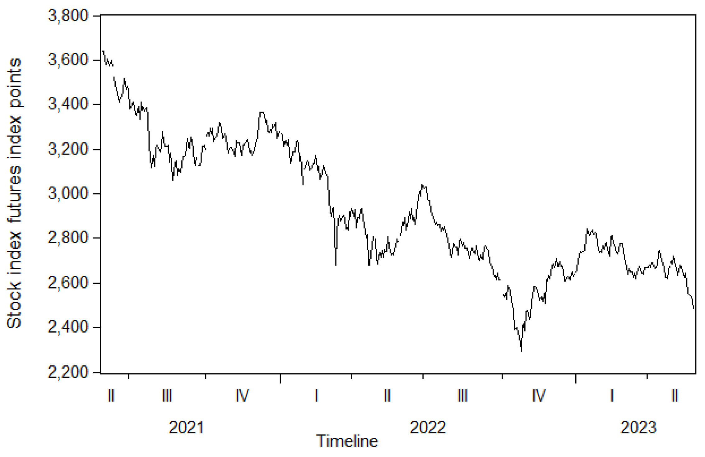
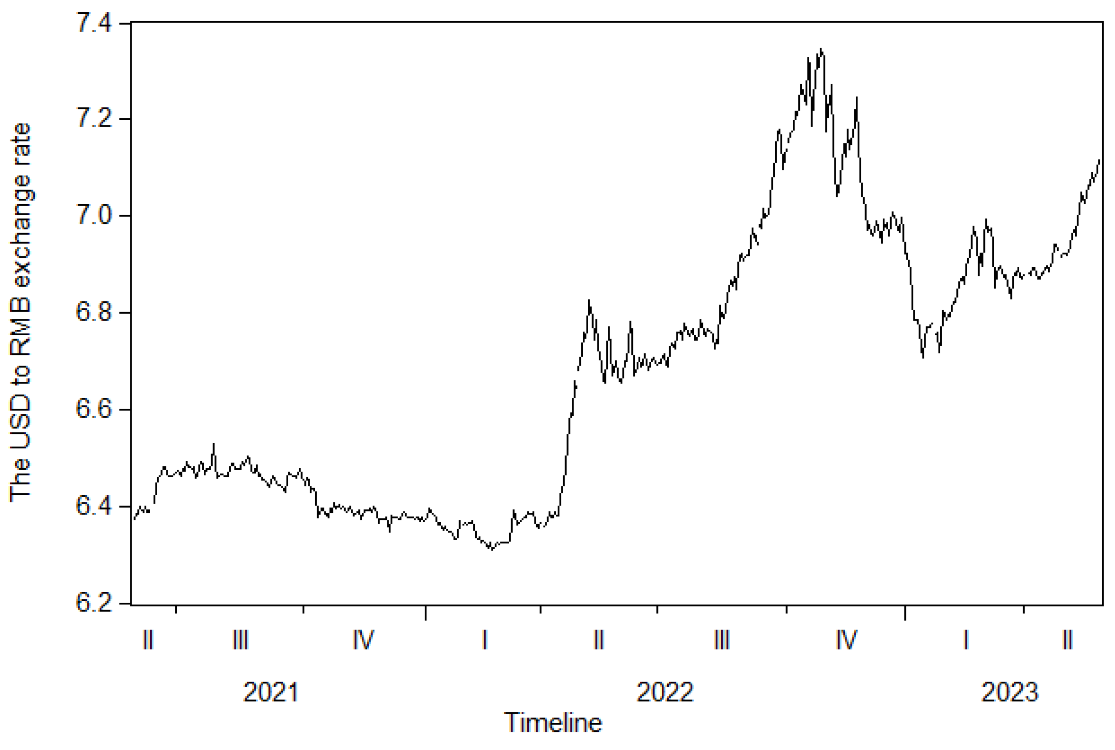
It can be seen in
Figure 1 and
Figure 2 that in the same period, under the influence of macroeconomic factors, when the price of the offshore RMB exchange rate rose, it represents a depreciation of the value of the people’s currency to a certain extent, the domestic macroeconomy was weakened, and the price of stock index futures declined. According to the calculations, the correlation coefficient is
, the offshore RMB exchange rate and stock index futures showed a certain negative correlation.
4.3. Descriptive Statistics
It can be seen in
Table 1 that the skewness of the return rate of stock index futures and the return rate of the offshore RMB exchange rate was less than zero, and the kurtosis was greater than 3, showing left-skewed, peak, and fat-tailed characteristics. The JB statistic illustrated that the stock index futures return series did not follow a normal distribution. The stationarity test of the return rate, relative trading volume, absolute return rate, volatility, and return of the offshore RMB exchange rate of stock index futures showed that all series were stationary according to the ADF value.
4.4. Determining the System’s Stability
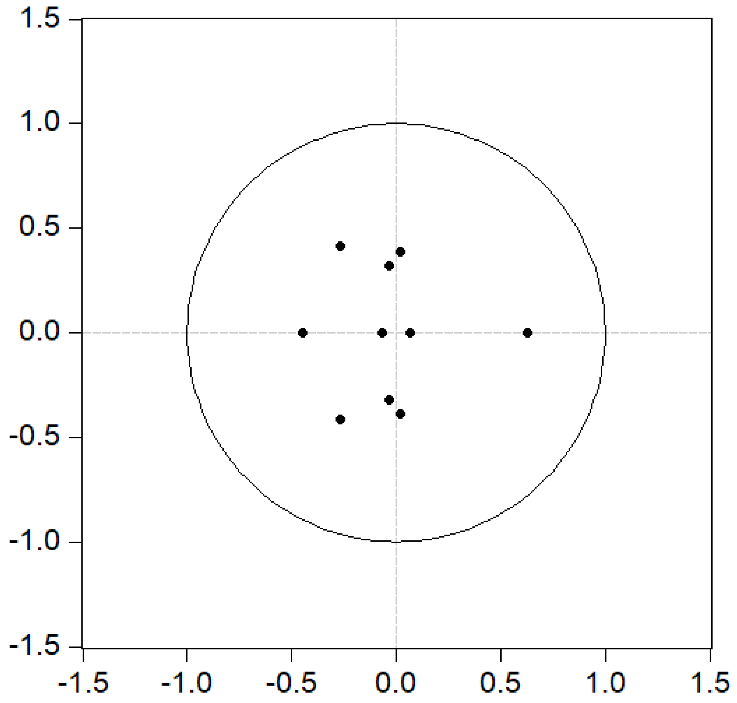
We constructed a VAR model to observe the dynamic relationship between the interactions and influences of these variables. Firstly, it was necessary to determine the lag order of the VAR model, and the optimal lag order could be determined by minimizing the AIC value and SC value of the information criterion at the same time. Then, a stationarity test of the established VAR model was carried out. It can be seen in the AR root diagram in
Figure 3 that all points fell within the unit circle, which indicated that the established VAR model was stationary, so the impulse response and variance decomposition analysis could be carried out. Further insight into the dynamic relationships among the variables is provided in the following.
4.5. Granger Causality Test
In order to understand the mutual guidance relationship between the return of stock index futures and the return of the offshore RMB exchange rate, stock index futures’ absolute return, price volatility, trading volume, and price volatility, it was necessary to conduct the Granger causality test after determining the best lag period. The test results are shown in
Table 2.
According to the results of the Granger causality test, it could be concluded that the offshore RMB exchange rate return was the Granger cause of the return of stock index futures, but the return of stock index futures was not the Granger cause of the offshore RMB exchange rate return, which indicated that the offshore RMB exchange rate return had a predictive effect on the return of stock index futures, but the return of stock index futures has no predictive effect on the offshore RMB exchange rate return.
There was bidirectional Granger causality between the volume of stock index futures and the volatility, that is, the volume of stock index futures was the Granger cause of the volatility, and the volatility was also the Granger cause of the volume of stock index futures, which indicated that the volume of stock index futures had a predictive effect on the volatility, and the volatility of stock index futures had a predictive effect on the volume.
There was bidirectional Granger causality between the absolute return and volatility of stock index futures. That is, the absolute return of stock index futures was the Granger cause of volatility, and the volatility of stock index futures was also the Granger cause of the absolute return of stock index futures, which indicated that the absolute return of stock index futures had a predictive effect on their volatility, and the volatility of stock index futures had a predictive effect on their absolute return.
There was no bidirectional Granger causality between the volatility of stock index futures and the offshore RMB exchange rate return. That is, the volatility of stock index futures is not the Granger cause of the offshore RMB exchange rate returns, and the offshore RMB exchange rate returns are not the Granger cause of the volatility of stock index futures, which indicates that there is no predictive effect between the volatility of stock index futures and the offshore RMB exchange rate returns.
4.6. Pulse Response Analysis
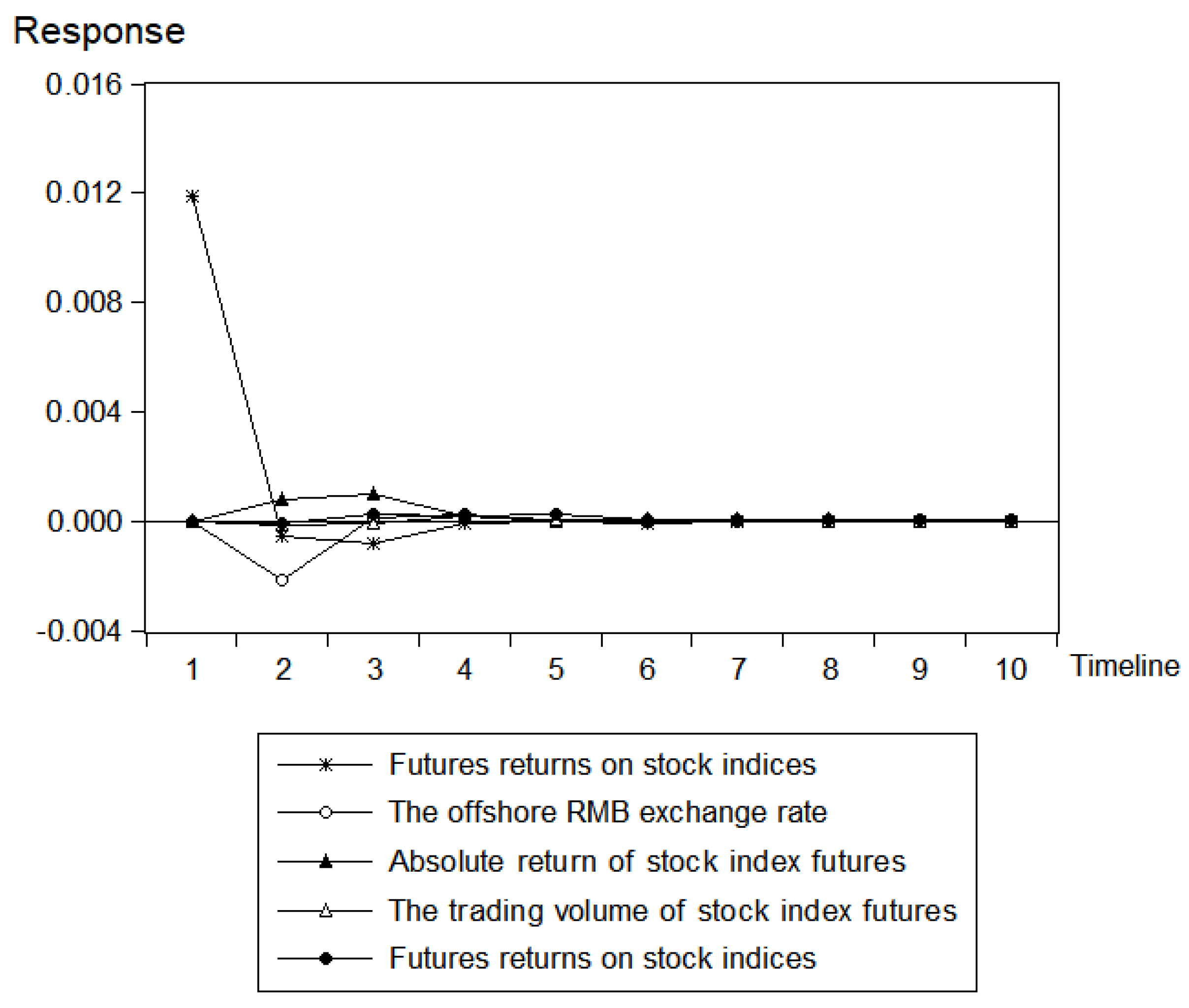
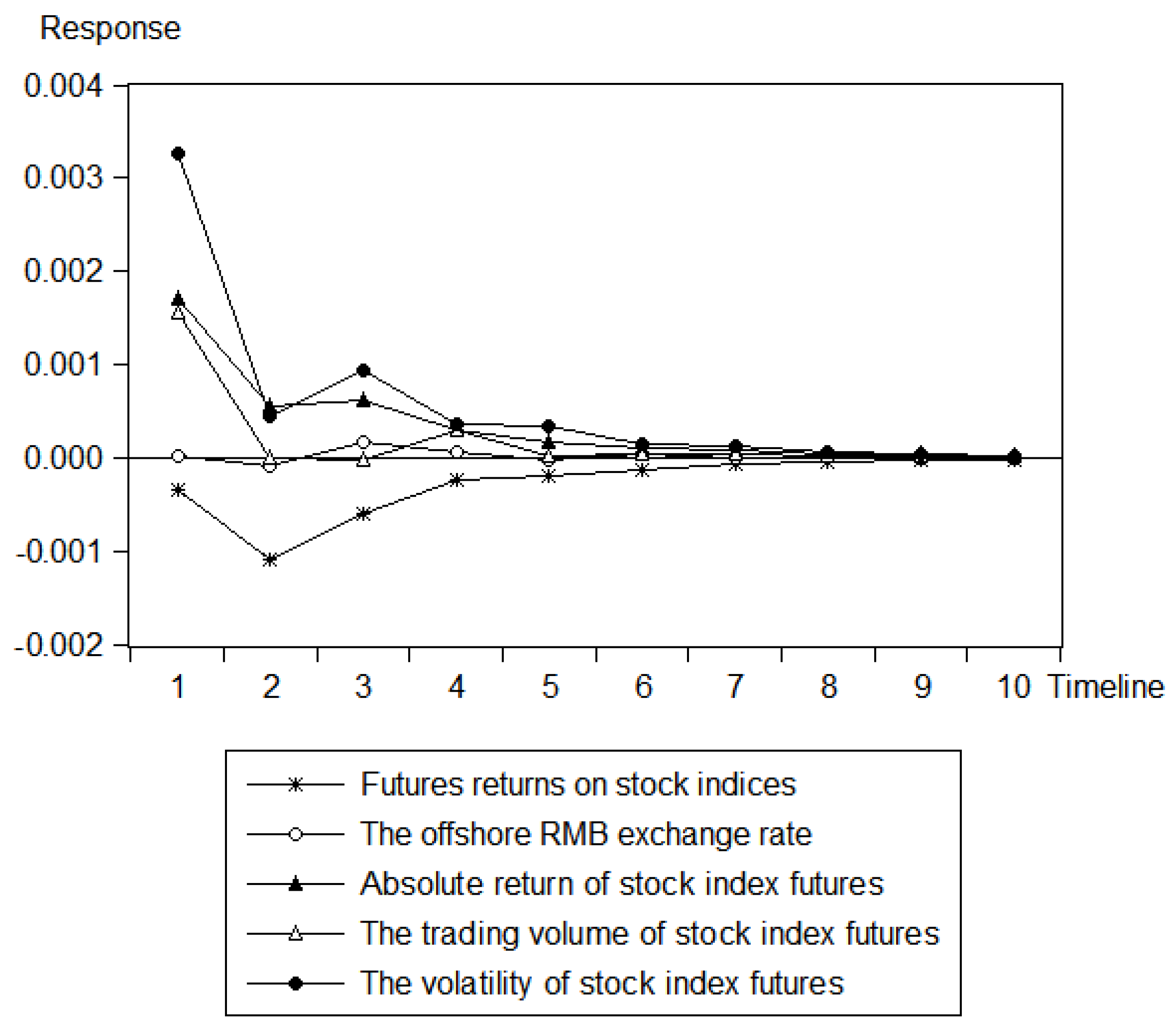
It can be seen in
Figure 4 that when the return rate of stock index futures was positively impacted by its own unit, the return rate of stock index futures rapidly decreased and became negative in the second period. Finally, the negative effect gradually disappeared, which indicates that the return rate of stock index futures was greatly influenced by itself. When the return of stock index futures was positively impacted by volatility and trading volume, the response of the return of stock index futures changed weakly on the zero axis, which indicated that volatility and trading volume had weak effects on it. When the return rate of stock index futures was positively impacted by the unit of the absolute return rate, the positive effect gradually became larger and reached the maximum in the third period, and the positive effect gradually decreased from the third period to the fourth period. This showed that the absolute return rate of stock index futures had a positive impact on the return rate of stock index futures at the beginning, and then the impact became smaller until the impact disappeared. When the return rate of stock index futures was negatively impacted by the return rate of the offshore RMB exchange rate, the return rate of stock index futures was 0 until the third period, which indicated that the offshore RMB exchange rate had a negative impact on stock index futures at the beginning, and the impact gradually disappeared after the third period.
It can be seen in
Figure 5 that the volatility of stock index futures was positively impacted by its own unit, and the volatility of stock index futures decreased from the first period to the second period. The response from the second period to the third period slowly rose, and the third period began to decline; finally, the impact disappeared, which indicated that the volatility from the first period to the second period had a great impact on itself; then, the volatility had a slow and continuous impact on itself. When the volatility of stock index futures was positively impacted by the volume unit, the volatility of stock index futures decreased from the first period to the second period, and the second period had a weak and slow response. This showed that the volume lags of one and two periods had a strong impact on volatility. When the volatility of stock index futures was positively impacted by the absolute return unit, the response of the volatility began to gradually and slowly decrease, which indicated that the absolute return rate had a continuous and slow impact on the volatility. When the volatility of stock index futures was positively impacted by the return of the offshore RMB exchange rate, the volatility had a weak positive response, which indicated that the return of the offshore RMB exchange rate had a weak impact on the volatility of stock index futures. When the volatility of stock index futures was negatively impacted by the return rate of stock index futures, the negative response of volatility gradually became larger from the first period to the second period, and the response gradually converged from the second period, which indicated that the return rate of stock index futures had a negative impact on the volatility of stock index futures.
4.7. Variance Decomposition
Variance decomposition is a method used to analyze time-series data. The basic idea is to decompose the total variance of a variable into variance components from different sources so as to reveal the degrees of influence of different factors on the variable. Specifically, variance decomposition divides the variance of a variable into two components: endogenous variance and exogenous variance. Endogenous variance represents the volatility of the variable itself, that is, the volatility component determined by itself, while the exogenous variance represents the volatility component of the variable that is affected by external factors. By performing variance decomposition, we can learn the extent to which different factors contribute to the volatility of the variables.
It can be seen in
Table 3 that with the increase in its own lag period, the contribution of the price volatility of stock index futures to its own volatility gradually decreased and, finally, basically stabilized the residual disturbance of about 61.46%. The contribution of the trading volume to volatility gradually decreased with the increase in its own lag order and, finally, stabilizes at the residual disturbance of 25.00%. With the increase in its own lag period, the contribution of the offshore RMB exchange rate to the volatility slowly increased and, finally, stabilized at the residual disturbance of about 0.896%. These five variable explanations were basically stable in period 8.
4.8. The Offshore RMB Exchange Rate and Stock Index Futures
To explore the impact of the offshore RMB exchange rate returns on the returns of stock index futures, we added offshore RMB exchange rate returns to the mean equation of GARCH (1,1) with the following model:
It can be concluded from the estimation results that when the offshore RMB exchange rate return was introduced into the GARCH model, the corresponding coefficient decreased, indicating that there was a certain relationship between the two, which may mean that the newly introduced variables had a certain explanatory effect on the dependent variable. According to the AIC criterion, the smaller the AIC value is, the more accurate the model estimation is. The AIC value of the original GARCH model was −6.055281, but the AIC value of the GARCH model with the addition of the trading volume was −6.073892, which showed that the GARCH model with the addition of the offshore RMB exchange rate was more accurate than the original model (
Table 4).
4.9. Trading Volume and Volatility of Stock Index Futures
The GARCH models are divided into the mean equation and variance equation. In order to explore the impact of the trading volume on volatility, the lagged term of the trading volume was added to the variance equation of GARCH(1,1); the following model was obtained:
From the estimation results, it can be concluded that the corresponding coefficient was greater than zero and statistically significant when the trading volume was introduced into the GARCH model, which indicated that the trading volume played a good role in explaining the volatility of stock index futures prices. According to the AIC criterion, the smaller the AIC value is, the more accurate the model’s estimation. The AIC value of the original GARCH model was −6.053631, and the AIC value of the GARCH model with added turnover was −6.054083. It can be seen from the AIC value that the GARCH model with added variables was more accurate than the original model (
Table 5).
4.10. Absolute Return Rate and Volatility of Stock Index Futures
In order to explore the impact of the absolute return of stock index futures on volatility, the lagged term of the absolute return was added to the variance equation of GARCH(1,1), and the following model was obtained (
Table 6):
It can be concluded from the estimation results that when the trading volume was introduced into the GARCH model, the corresponding coefficient decreased and was statistically significant, indicating that there was a certain relationship between the two, which may mean that the newly introduced variable had a certain explanatory effect on the dependent variable, indicating that the absolute return rate had a good explanatory effect on the volatility of stock index futures prices. According to the AIC criterion, the smaller the AIC value is, the more accurate the model’s estimation. The AIC value of the original GARCH model was −6.053631, and the AIC value of the GARCH model with the absolute return was −6.589577. It can be seen from the AIC value that the GARCH model with the absolute return was more accurate than the original model.


