1. Introduction
Optimization refers to the design of existing schemes and parameters under given conditions so that a problem can obtain a more satisfactory answer. Optimization problems are often encountered in scientific research and production practice [
1]. For a long time, scholars have conducted a lot of research on optimization problems and expanded optimization problems, making this a critical discipline. In the 17th century, Newton and Leibniz founded calculus and successfully solved a difficult problem, which can be regarded as a milestone in optimization theory. Then, the Lagrange multiplier method, the steepest descent method, the linear programming method, and the simplex method were proposed. These mathematical theories have been widely used in various engineering systems, economic systems, and social systems. However, these methods are aimed at particular problems and have specific requirements for their searching spaces. The objective function must be set as convex, continuously differentiable, and differentiable. With the development of science and technology, there are a large number of optimization problems to be solved in many practical application fields, such as the distribution center location problem, the layout optimization of factory production, the optimal allocation of equipment resources, the product scheduling problem, etc. [
2,
3,
4].
These practical problems are generally large-scale, nonlinear, and multipolar, and many industrial optimization problems should be solved under complex variable conditions and over large search ranges. The traditional optimization method cannot carry out mathematical modeling. Therefore, exploring intelligent optimization methods for large-scale computing has become an important research direction in related disciplines. Therefore, industry and mathematics need strong computing power and high-precision optimization strategies to solve complex optimization problems, including nonlinear, multivariable, multi-constraint, and multi-dimensional problems. As an important branch of artificial intelligence fields, the intelligent optimization algorithm is a new evolutionary computing technology that has attracted more and more attention from scholars. The main idea of the intelligent optimization algorithm is to construct a searching algorithm according to natural characteristics. To create an intelligent optimization algorithm, metaheuristic optimization algorithms have been applied to mathematical methods to search for feasible solutions to linear and nonlinear function problems [
5,
6,
7]. In recent years, intelligent optimization algorithms have been widely applied in different fields [
8,
9,
10]. Many optimization algorithms have been designed by scholars to solve complex optimization problems, such as, Poor and Rich Optimization (PRO) [
11], Beluga Whale Optimization (BWO) [
12], Monarch Butterfly Optimization (MBO) [
13], Student Psychology-Based Optimization (SPBO) [
14], Jellyfish Search (JS) [
15], etc. [
16,
17,
18,
19,
20].
These algorithms can obtain acceptable solutions in a limited computing time and can obtain empirical information in the searching process. Additionally, optimization algorithms rely on optimization rules, which makes them less demanding in terms of mathematical properties. At the same time, due to the algorithms’ searching ability, they can significantly reduce searching times for large-scale problems. The Flow Direction Algorithm (FDA), which was proposed by Hojat Karami in 2021, is physics-based. FDA is inspired by the movement of water into the outflow in a catchment area. The FDA shows the flow direction to the outlet point with the lowest height in a drainage basin. The flow moves to the neighbor with the best objective function [
21,
22]. To further improve the searching ability, iteration speed, and jumping out power of the optimal local solution in the basic FDA, this paper proposed an improved FDA based on the Lévy flight strategy and the self-renewable method (LSRFDA). New coefficient factors based on the Lévy flight strategy and the self-renewable method were added to the basic FDA. These two methods enabled the LSFDA to find better feasible solutions and achieve a faster speed. To weaken the disadvantages of the standard FDA, this paper proposed an improved FDA based on the Lévy flight strategy and the self-renewable method (LSRFDA)., which could effectively improve its solving accuracy and the convergence performance of complex functions in spaces with different dimensions. Secondly, we introduced the LSRFDA to engineering optimization problems, and compared it with other algorithms to show that the model proposed in this paper has good robustness and generalization ability. The LSRFDA uses the Lévy flight strategy and the self-renewable method to strengthen its searching ability and iteration speed, and can jump out of the optimal local solution. In this paper, an improved FDA algorithm is proposed to solve engineering optimization problems. The LSRFDA focuses on improving upon some disadvantages of basic FDA in the searching process, and on solving engineering optimization problems; thus, it could provide new methods of solving engineering optimization problems. For function experiments, this paper applied different functions to test the proposed algorithm. Iteration curves, box plot charts, and search path figures were created, and the Wilcoxon rank sum test conducted. The rest of this paper is organized as follows: In
Section 2, this paper introduces the basic FDA. In
Section 3, this paper presents the proposed LSRFDA. In
Section 4, the function experimental parameters, function experimental environments, numerical calculation results analysis, algorithm sub-sequence calculation results analysis, Wilcoxon rank sum test results analysis, iteration results analysis, box plot results analysis, and searching path results analysis are shown. In
Section 5, the engineering optimization problems are given. In
Section 6, the discussion is presented. In
Section 7, the conclusion is given.
2. Flow Direction Algorithm
Concerning the FDA, the position of the initial flow is determined based on the following relationship:
where
Flow_X(
i) means the position of the
i-th flow,
lb and
ub mean the lower and upper limits of the decision variables, and the parameter rand is in the range of [0, 1]. There are neighborhoods around each flow, and the neighbor flow position is created based on the following relationship:
where
Neighbor_X(
i) represents the
j-th neighbor position, and
randn is a random value with a normal distribution in the range of [0, 1].
where the parameter rand is in the range of [0, 1],
Best_X is the global optimal solution, and
Xrand is a random position that is created based on the following relationship:
where the parameters
rd,
Rm, Δ
t, and
M mean the amount of direct runoff, rainfall, time interval, and the number of time steps, respectively.
where
is a random vector with uniform distribution,
iter means the current iteration, and
Max_iter means the global iteration.
The following relationship is applied to complete the new position of the flow:
where Flow
_newX(
i) shows the
i-th new flow position.
where
Flow_fitness(
i) and
Neighbor_fitness(
j) represent different values of the
i-th flow and the
j-th neighbor, respectively. The parameter d represents the problem dimension. Then, we generate a random integer number
r.The flow will move to the
r-
th flow if the fitness of the
r-
th flow is less than the fitness of the current flow. The following relationship shows how to mimic the flow direction in these conditions:
The FDA’s iterative process is as follows:
Step 1. In the initialization phase, the algorithm randomly generates an initial population of flows, defines the objective function and its solution space, and finds the best objective function and the best solution. Set the maximum iterations Max_Iter. Set iter = 1.
Step 2. Create the neighbor flow position in Formula (2) and Δ in Formula (3) for each individual of the population or flows.
Step 3. Calculate each objective function value. Record the best neighbor solution value, and the best global optimal solution value in the current generation. If the best neighbor has a better objective function than the current flow, proceed to step 5. Otherwise, go to step 6.
Step 5. Find the new flow position according to Formula (6).
Step 6. Update the flow position according to Formula (9).
Step 7. Find the best objective function value and the best solution in the current generation. Replace the global solution and the global value if there is a better solution.
Step 8. Calculate iter = iter + 1. Judge whether iter equals Max_Iter. If not, return to step 2 and continue. Otherwise, stop the iteration.
3. The Proposed Algorithm
To obtain a better search result in the FDA, this paper introduces an improved FDA based on the Lévy flight strategy and the self-renewable method (LSRFDA). The Lévy flight strategy and the self-renewable method are added the original algorithm. In the proposed algorithm, iteration is optimized through mutual cooperation and a global information sharing mechanism. Global searching enables the algorithm to quickly find the optimal solution, while local searching enables the algorithm to thoroughly use the information around the optimal solution to find a better solution. The Lévy flight strategy was proposed by French mathematician Lévy according to non-Gaussian random moving in 1925. Lévy flight defines a scale-invariant walking model, which can be redefined by connecting the long gait with the small gait since the Lévy distribution is a non-Gaussian random process [
23,
24]. The probability density distribution of the Lévy flight strategy can be calculated based on the following relationship:
where
sL is the Lévy flight length and
β is the power law index, where 1 <
β ≤ 3. The Lévy flight strategy step is determined according to a random probability, showing a dynamic motion process. The parameters can be calculated as follows:
where
u~
N (0,
),
v~
N (0,
), and
σv = 1.
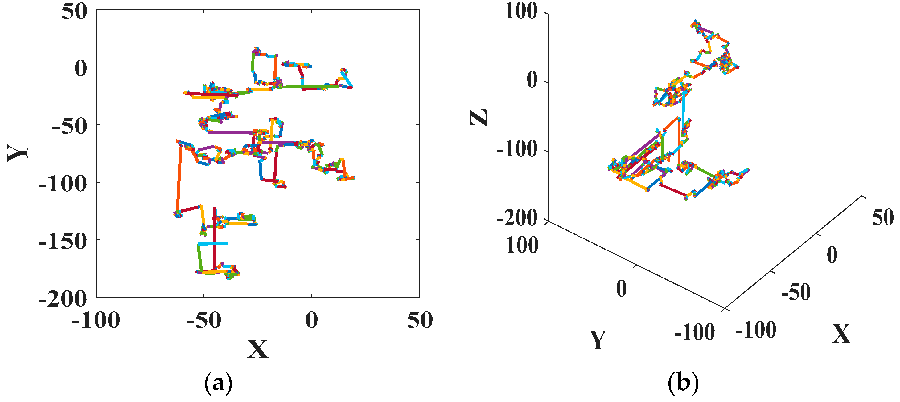
In this paper, the Lévy flight strategy is the most important stage of the methodology. So, this paper shows a two-dimensional Lévy flight path and a three-dimensional Lévy flight path in
Figure 1.
Thus, the Δ direction based on the Lévy flight strategy in this paper can be updated as follows:
This new
V based on the Lévy flight strategy can be updated using (14).
The self-renewable method can enable the algorithm to quickly obtain a better feasible solution, and can conduct a more detailed search for a feasible solution. The relationship that illustrates how to simulate the flow direction can be updated as follows:
The LSRFDA steps are summarized in the pseudo-code shown in Algorithm 1.
| Algorithm 1: LSRFDA |
1: Input: Function f(.). Searching range. Max_Iter. Set iter = 1. Flows N, Neighbors M.
2: Initial optimum solution Best_X. lb, ub, β = 1.5.
3: Output: Best_X.
4: While (iter < Max_Iter)
5: For 1 i = 1:N
6: For 2 j = 1:M
7: sL = u/(|v|1/β)
8: Flow_X(j) = lb + rand × (ub − lb)
9: Δnew = (rand × Xrand − rand × Flow_X(j)) × ||Best_X − Flow_X(j)|| × sL
10: Determining the best neighbor.
11: End For 2
12: If 1 the best neighbor has a better objective function than that of the current flow
13: Vnew = sL × So
14: Else
15: Generate random integer number r
16: If 2 Flow_fitness(r) < Flow_fitness(i)
17: Flow_newX(i) = sL × Best_X
18: Else
19: Flow_newX(i) = Flow_X(i) + sL × (Best_X − Flow_X(i))
20: End If 2
21: End If 1
22: Update Best_X if there is a better solution
23: End For 1
24: iter = iter + 1
25: End While |
The LSRFDA iterative process can be presented as follows:
Step 1. In the initialization phase, the algorithm randomly generates an initial population of flows, defines the objective function and its solution space, and finds the best objective function and best solution. Set the maximum number of iterations Max_Iter. Set iter = 1.
Step 2. Create the neighbor flow position, and the new Δ can be updated using Formula (13).
Step 3. Calculate each function value. Record the best neighbor solution value and the best global optimal solution value. If the best neighbor has a better objective function than that of the current flow, proceed to step 5, otherwise, jump to step 6.
Step 5. Calculate Formula (14) and find the new flow position according to Formula (15).
Step 6. Update the flow position according to Formula (16).
Step 7. Find the best objective function value and the best solution in the current generation. Replace the global solution and the global function value if there is a better solution.
Step 8. Calculate iter = iter + 1. Judge whether iter equals Max_Iter. If not, return to step 2 and continue. Otherwise, stop the iteration.
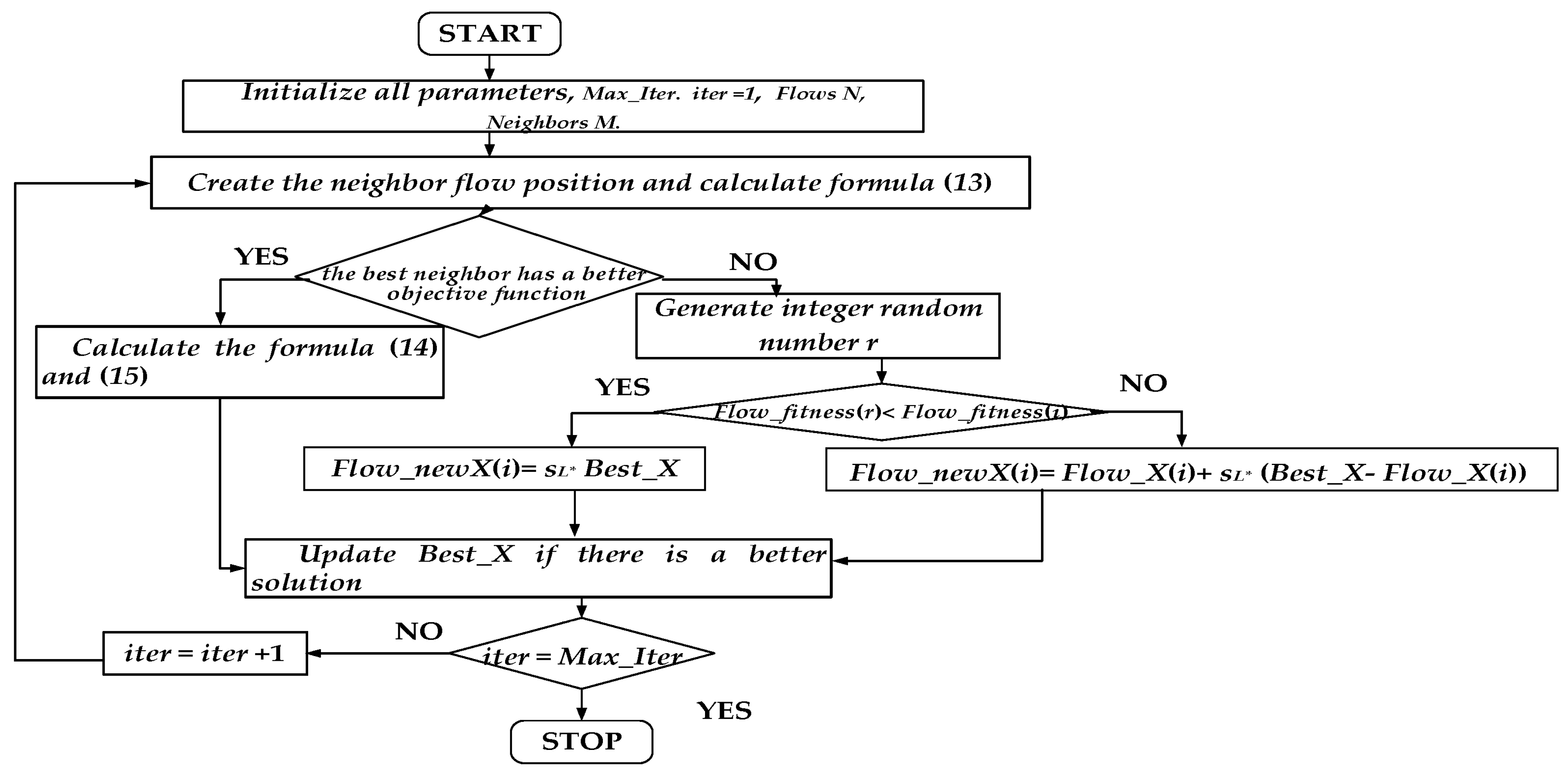
The main SRLFDA flow chart is shown in
Figure 2.
4. Function Experiments
4.1. Testing Environments
To verify the searching ability of the proposed algorithm for solving complex functions with different dimensions, this paper carried out mathematical benchmark function experiments.
Table 1 shows the low-dimensional and variable-dimensional benchmark functions, where
f1 to
f10 are low-dimensional functions and
f11 to
f16 are variable-dimensional functions.
In
Table 1,
D represents the dimension,
fmin is the ideal optimal value, and
Range is the searching scope. The original FDA literature already compared some intelligence algorithms, so this paper selects other algorithms for comparative experiments to avoid repeated and unnecessary experiments. The compared algorithms include Moth–Flame Optimization (MFO) [
25], a Multi-Verse Optimizer (MVO) [
26], Simulated Annealing (SA) [
27], and basic FDA. MFO, which was proposed in 2015 by Seyedali Mirjalili, is based on the moth navigation method in nature called transverse orientation. The inspirations for MVO are based on three concepts, including the white hole, the black hole, and the wormhole. In MVO,
r2,
r3, and
r4 are in the range of [0, 1]. SA is a probability algorithm derived from the solid annealing principle. SA includes two initial parameters, including initial temperature
t0 and attenuation factor k. In this paper,
t0 is set at 100, and k is set at 0.95. All the iterative processes and details of the compared algorithms can be found in the original algorithm literature. All the initial parameters of the compared algorithms were selected based on the original algorithm literature. This paper sets the population size of all the algorithms to 50 and sets the maximum iteration number of all the algorithms to 200. To obtain a fair result and remove randomness, all the algorithms were run independently 10 times. All the programs, data, and figures were accomplished in MATLAB (R2014b). The key feature parameters of all the algorithms used in this comparative study are shown in
Table 2. Max_Iter is the maximum iteration number. N means the population size.
4.2. Numerical Calculation Results Analysis
To verify the effectiveness of the improved algorithm in this paper, this chapter selects the four indicators to comprehensively evaluate the competitiveness of the different algorithms. The three indicators include the highest searching value (Min), the lowest searching value (Max), and the average searching value (Ave).
Table 3 shows the two-dimensional function results.
Table 4 shows the high-dimensional function results (30/60/150). It can be seen from
Table 3 and
Table 4, that most of the calculated optimal values of the proposed algorithms in this paper are very close to the ideal optimal values in
Table 1. For the Min indicator, the LSRFDA has all the best searching values of all the comparison algorithms. For the Max indicator and the Ave indicator, the LSRFDA has the best searching values across all the benchmark function results, except
f10. In
f10, the FDA has the best Max indicator and the best Ave indicator. From
Table 3 and
Table 4, it can be seen that except for
f10, the LSRFDA proposed in this article is significantly superior to the other four comparison algorithms. For the
f10 function, the search result is not the best value, and the maximum value and the average value are slightly worse than the FDA but are better than MFO, MVO, and SA. Although the searching accuracy of the proposed algorithm will decrease with an increase in the test function dimension, the optimization efficiency and calculation power of the proposed algorithm are always better than those of the other comparison algorithms. The search results show that the LSRFDA can not only obtain the best target, but also has strong searchability. The optimization accuracy of the original FDA is low in the searching process, and the individual population in the FDA quickly falls into the local optimal solution area in the searching space. Although the basic FDA can obtain better results in some benchmark functions, when the benchmark function dimension is increased, the solution accuracy of the feasible solution in the FDA is significantly reduced. The numerical results of benchmark functions of different dimensions show that the proposed algorithms in this paper can efficiently find the optimal value of the benchmark function in a multi-dimensional searching space. The improved algorithm has high searchability, strong detection accuracy, and a fast iteration speed.
4.3. Sub-Sequence Run Results Analysis
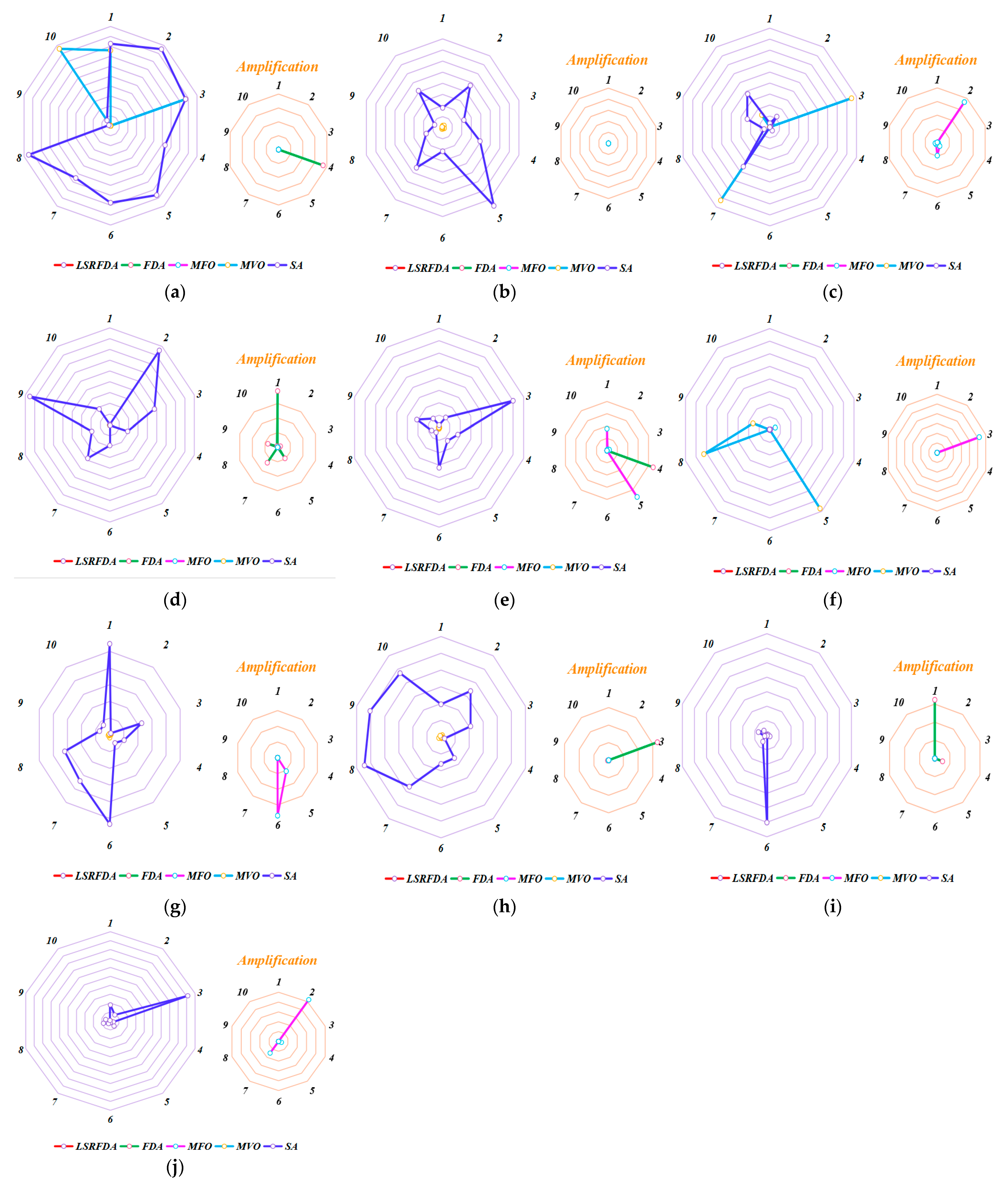
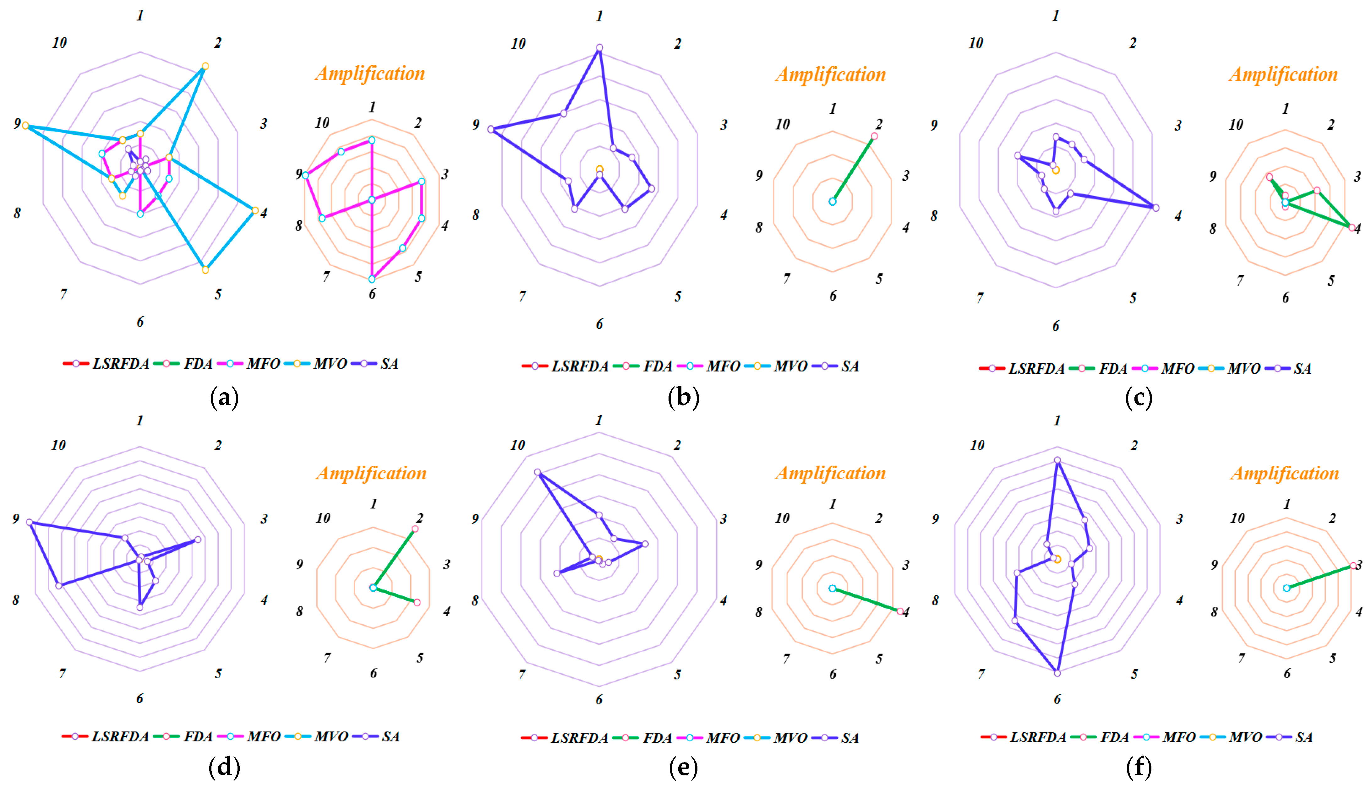
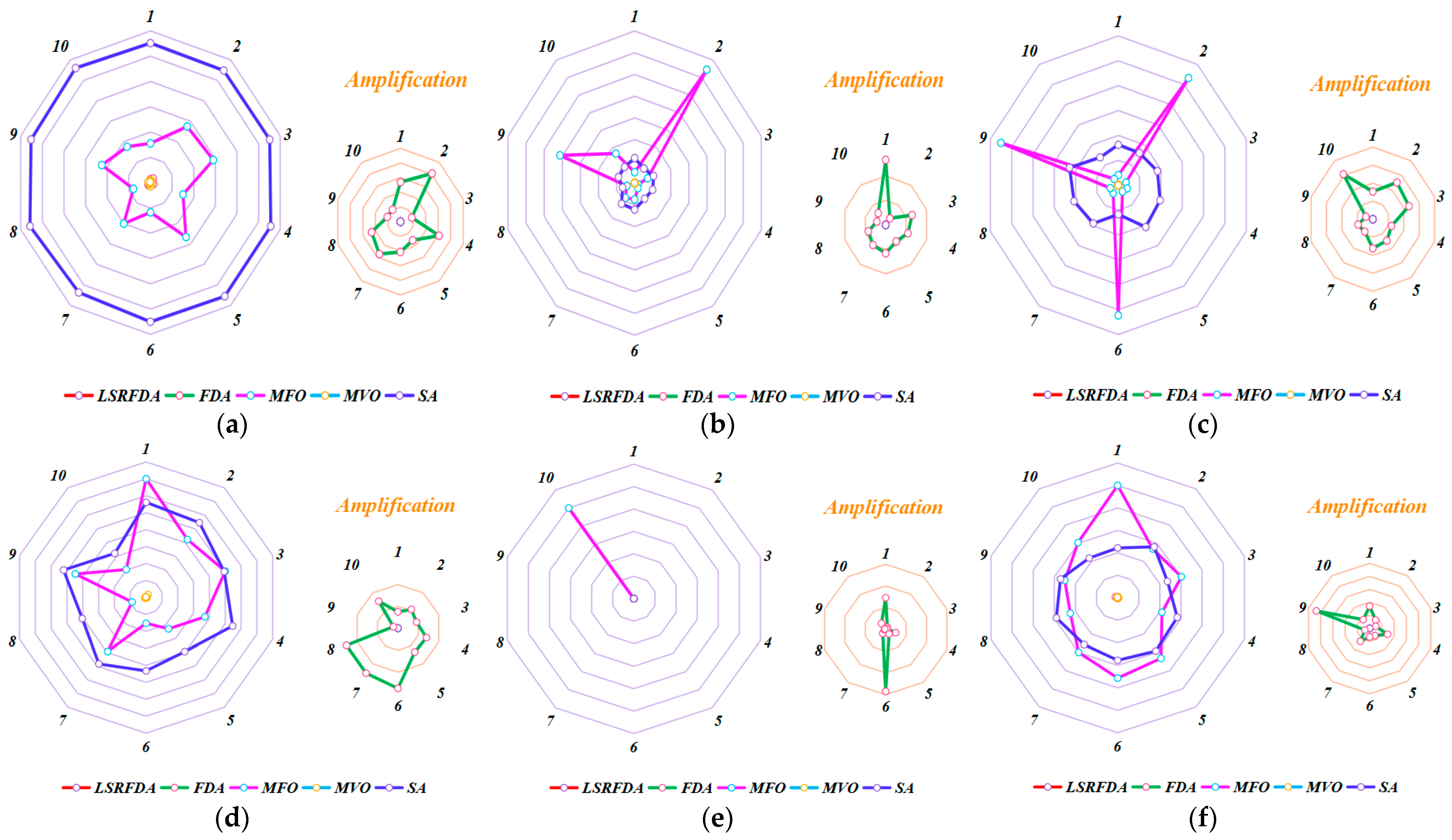
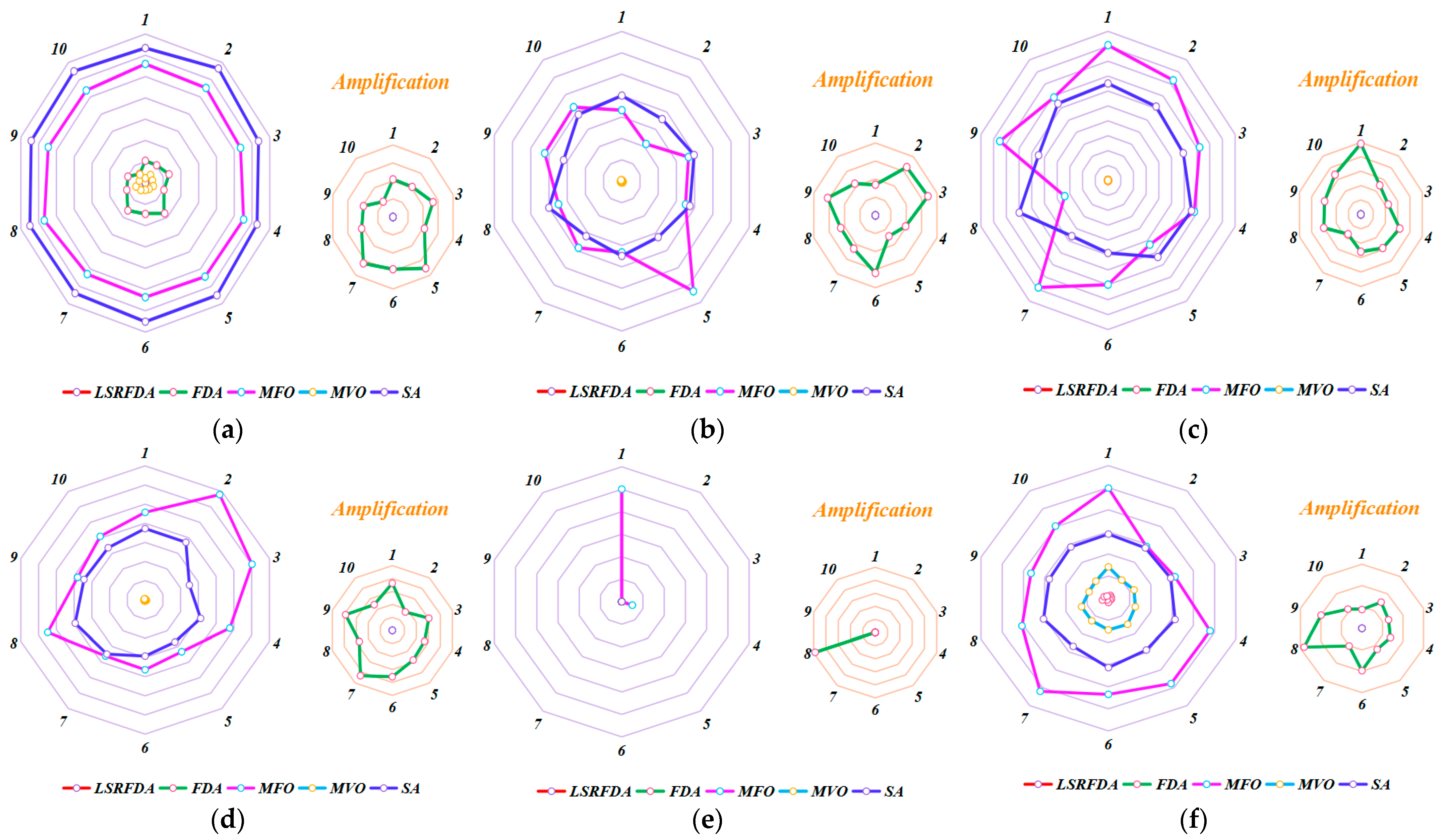
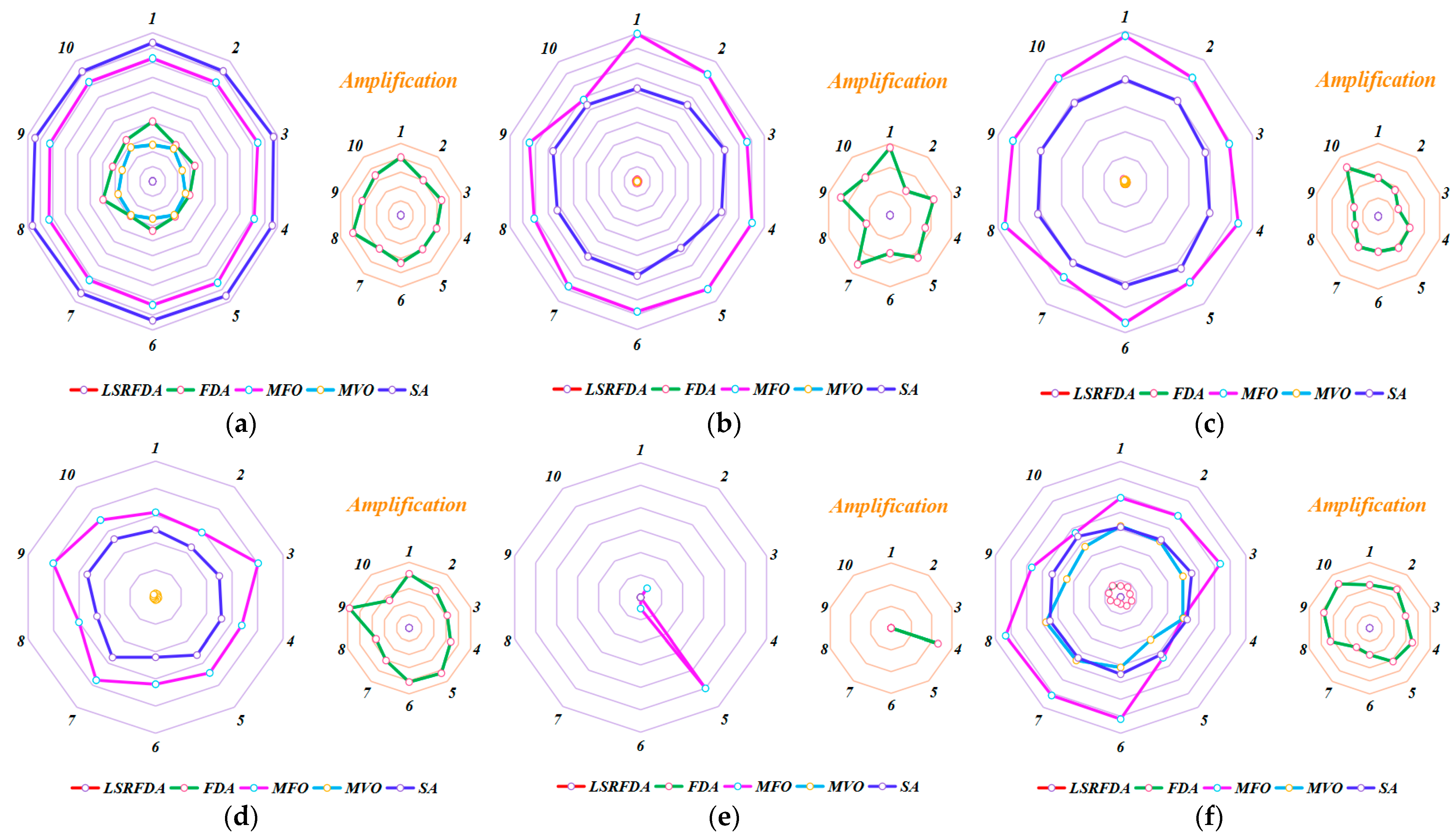
We conducted a basic statistical assessment of the results obtained in the sub-sequence runs of the algorithm. Radar charts of the algorithm’s 10 sub-sequence runs are shown in
Figure 3,
Figure 4,
Figure 5,
Figure 6 and
Figure 7. A radar chart is a graphical method used to display multivariable data in the form of a two-dimensional chart on an axis from the same point. The relative position and the angle of an axis are usually uninform. A radar chart is also called a network map, a spider map, a star map, a polar coordinate map, and a Kiviat map. The method involves draw corresponding function value ratio lines in a radial form, starting from the center of a circle, in different regions. Then, by connecting the corresponding function value ratio lines with lines, an irregular closed-loop graph is formed. In this paper, the radar chart clearly shows the running results of the algorithm sub-sequences and shows differences in the algorithm sub-sequences. If the edge of the radar chart is wider, the accuracy of the algorithm operation is lower. For two-dimensional functions, SA sub-sequences have large radar charts, except for
f3,
f6, and
f11(D=2). For high-dimensional functions (
D = 30/60/150), MFO and SA sub-sequences have large radar charts. LSRFDA sub-sequences have the smallest radar charts of all the functions. The radar charts show that LSRFDA can improve the searching ability of the basic FDA for in terms of its global searching and local exploration capabilities, can avoid the algorithm getting stuck in the local optimal solution, and can jump out of the local optimal region, which can improve the performance and solution accuracy of the basic FDA.
4.4. Wilcoxon Rank Sum Test Results Analysis
In the case of arbitrary distribution, the mathematical analysis method often uses symbol testing methods to verify whether there is a significant difference in the distribution positions of the paired experimental data. However, the symbol testing method only considers positive and negative signs of differences, without considering absolute differences in differences, which can result in the partial loss of experimental information and inaccurate results. To avoid this flaw in the symbol testing method, this paper uses the Wilcoxon rank sum test. This method considers both the direction and magnitude of differences, making it more effective than symbol testing. Similar methods can also be used to test whether there are differences in the distribution positions of the group of experimental data. The Wilcoxon rank sum test is based on the rank sum of sample data. First, two samples are regarded as a single sample. Then, observations are ranked from small to large. If it is true to assume that the two independent samples are from the same population, the rank will be approximately distributed from the two samples. If it is true to assume that the two independent samples come from different populations, one will have smaller rank values. The other sample will have larger rank values, so a large rank sum will be obtained. The Wilcoxon rank sum test can give
p values; if the
p value is less than 0.05, there is a significant difference at a level of 0.05. To further compare the proposed algorithm with the other algorithms, the Wilcoxon rank sum test was used in this paper. All of the algorithm’s
p values are given in
Table 5, and
NO means that the calculation results are not a number. For the FDA, the
p values of
f3,
f5,
f10,
f11(D=2), and
f16(D=2) are larger than 0.05. The other algorithms’
p values are less than 0.05. The Wilcoxon rank sum test shows that the LSRFDA has a large searching ability, which further shows that the LSRFDA has good searching performance. The LSRFDA performs significantly better than other comparison algorithms in solving different function problems. The Wilcoxon rank sum test results show that the range of optimal value fluctuation is very small, and the LSRFDA’s stability is strong. It can be seen that the proposed algorithm in this paper has good optimization performance for various typical functions, and has broad adaptability and strong robustness.
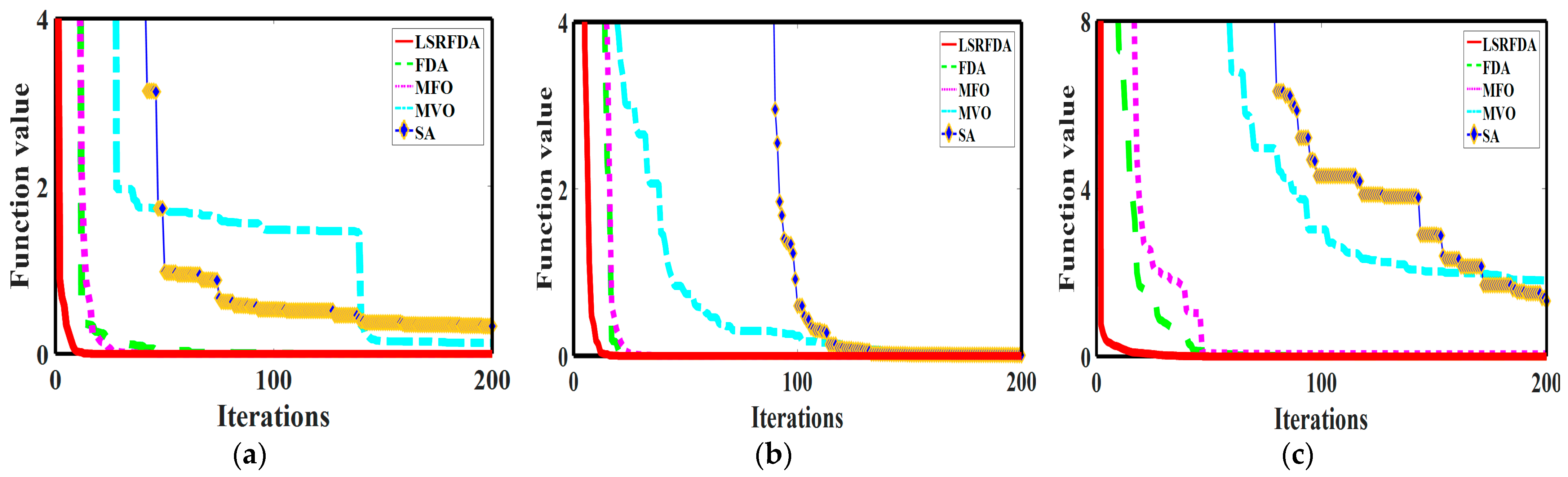
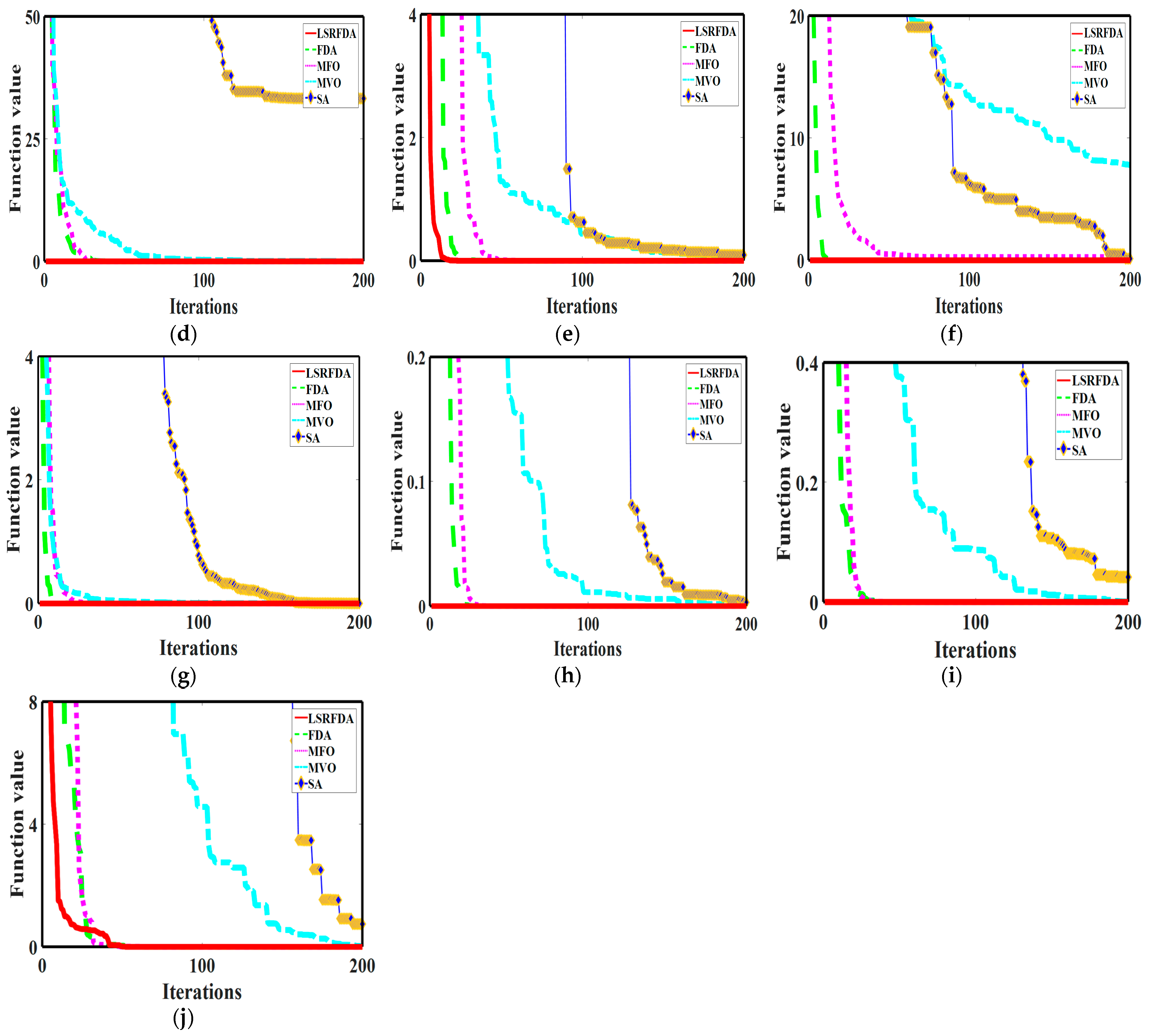
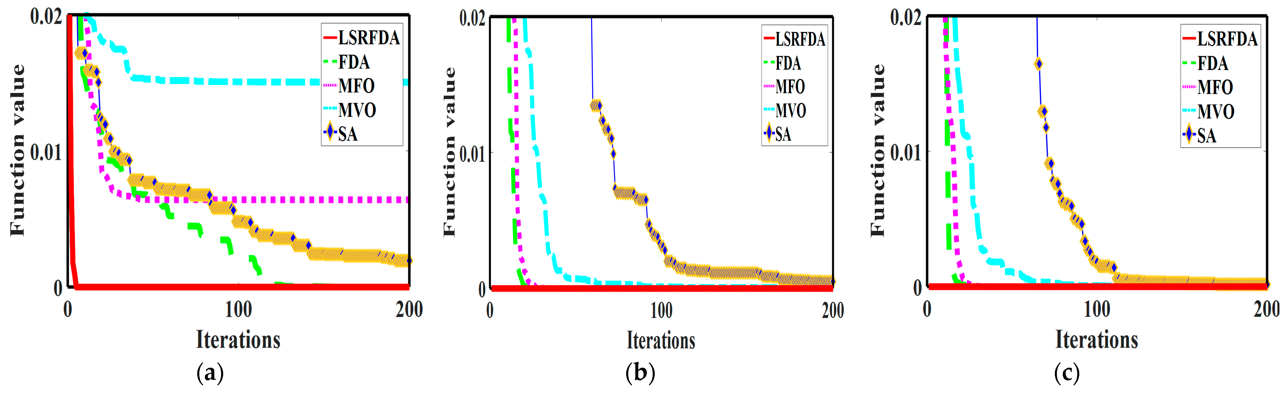
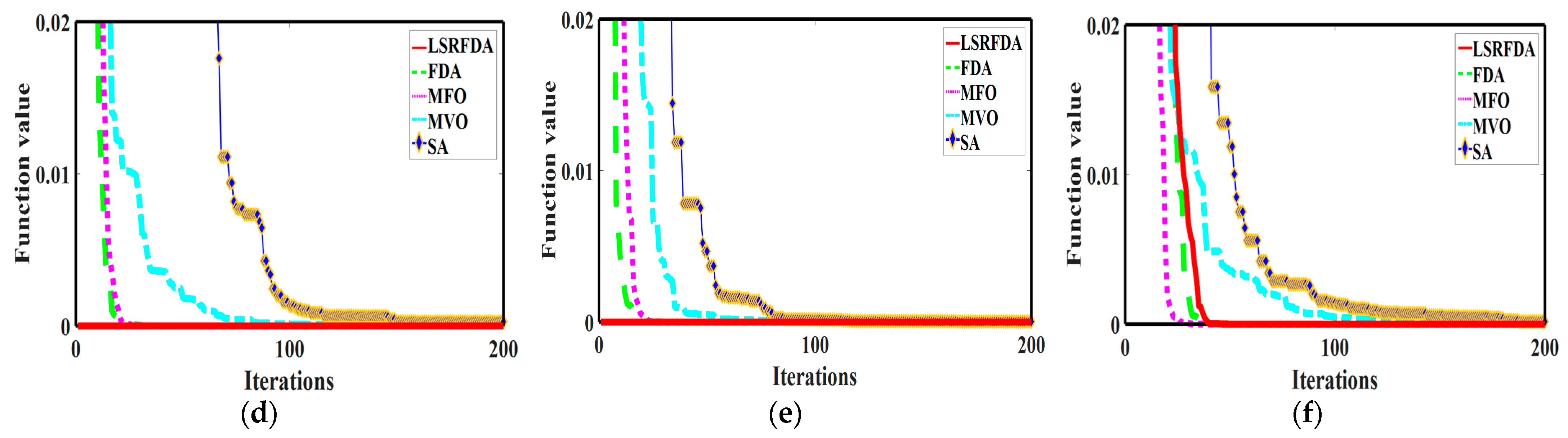
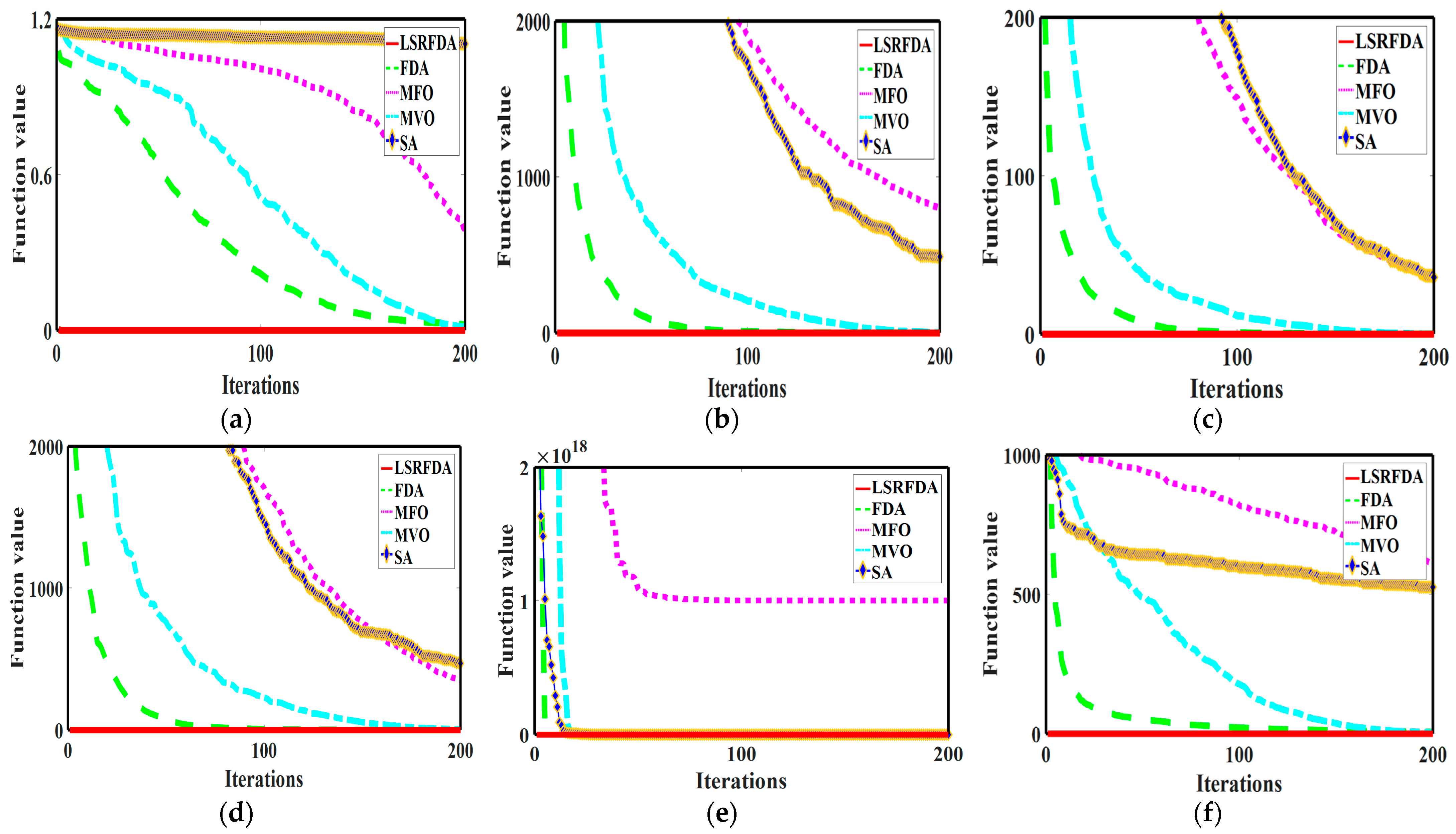
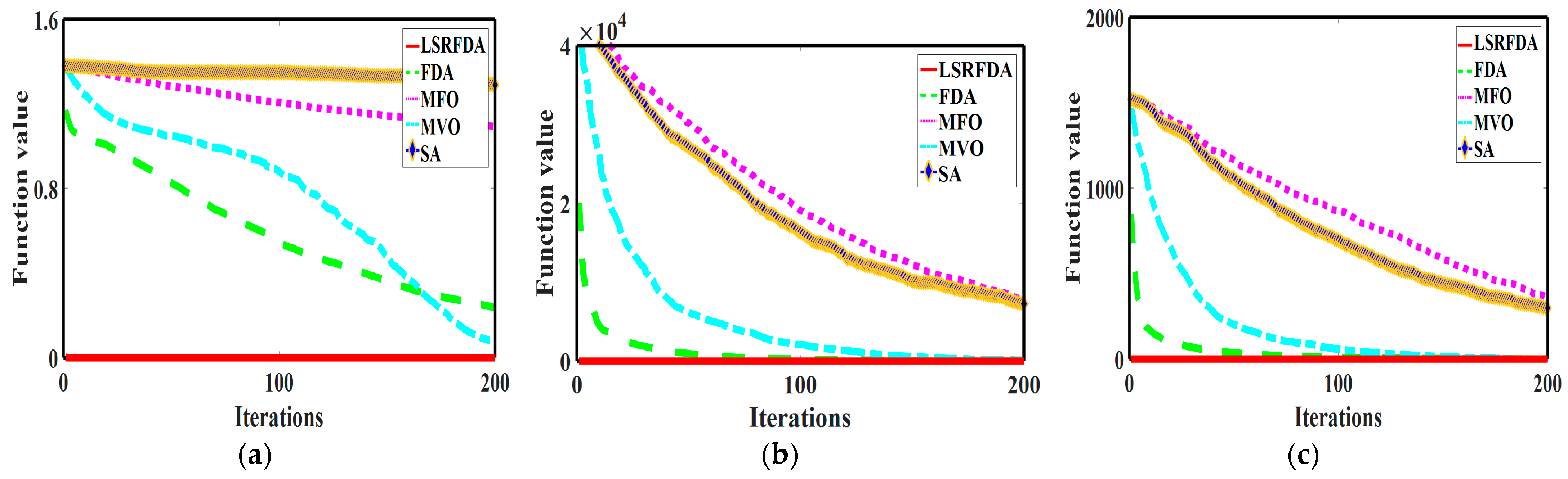
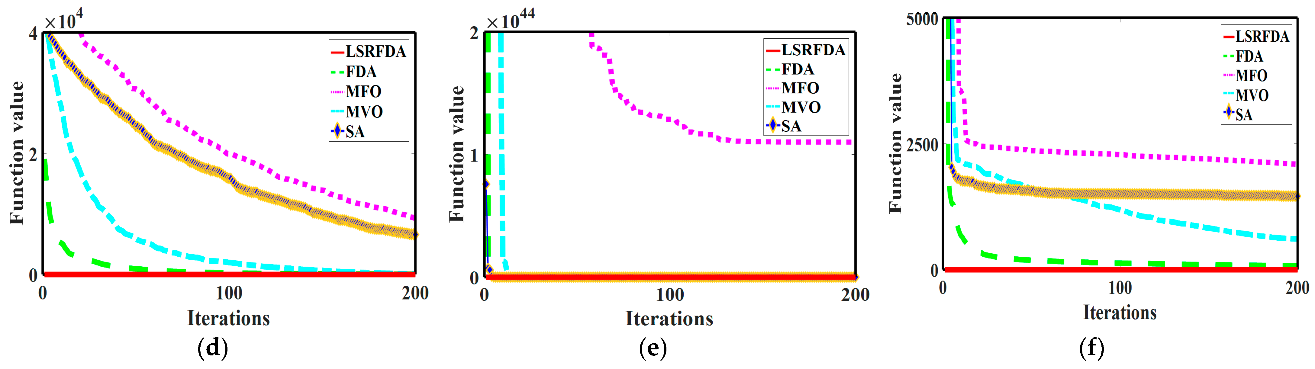
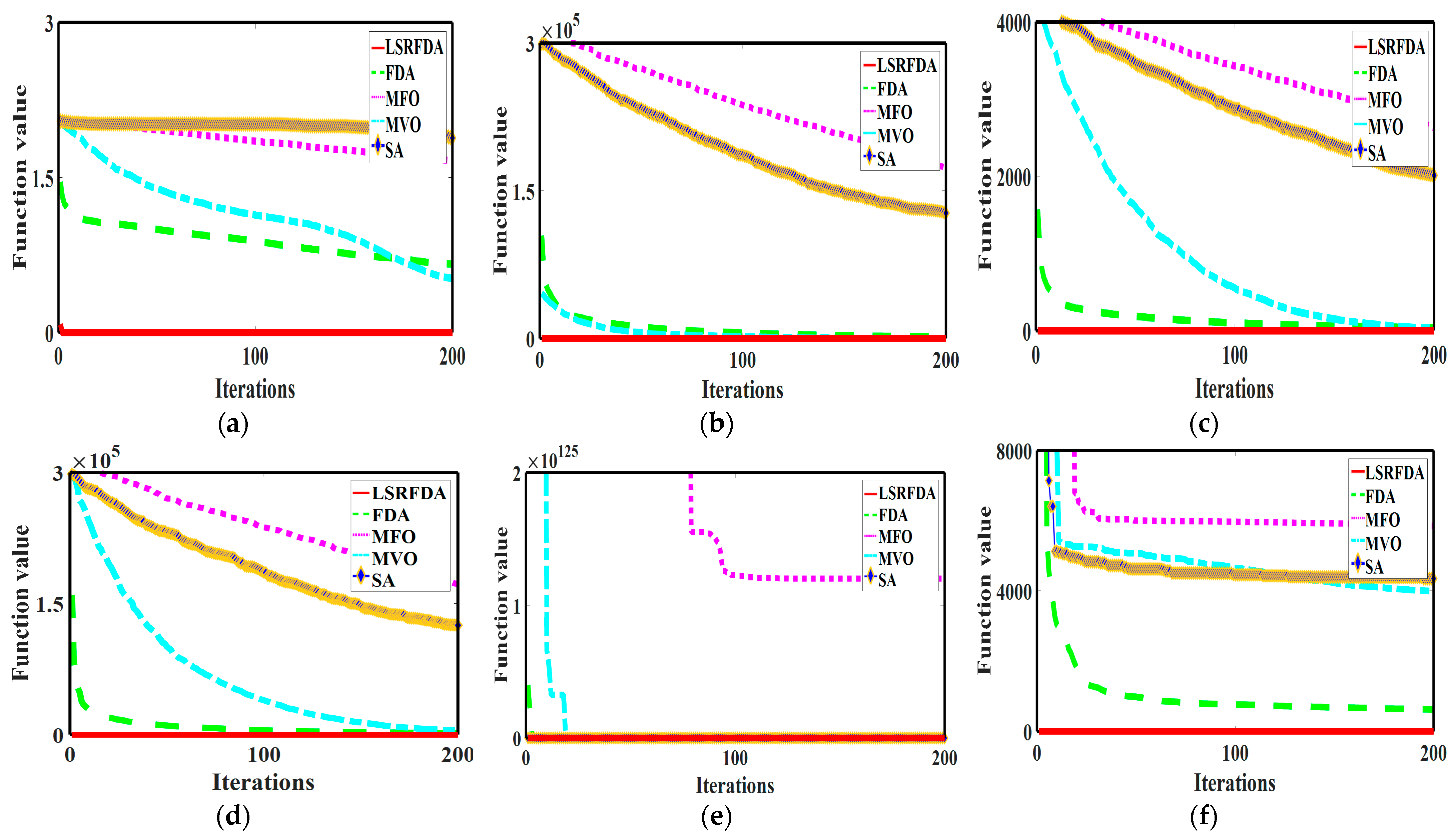
4.5. Iteration Results Analysis
Figure 8,
Figure 9,
Figure 10,
Figure 11 and
Figure 12 show the iterative results of different algorithms in benchmark functions of different dimensions. For all the functions, the iteration speed of the proposed algorithm is significantly faster than that of the basic algorithm. The LSRFDA can search on the left and right sides of the optimal value through the initial large searching step, and can skip a certain range of obstacles in the process. The convergence speed of the basic FDA algorithm is fast in the initial stage of iteration. Still, the individual population in the FDA will fall into the local optimal solution region and cannot jump out with the optimization iteration. The LSRFDA significantly improves the population diversity, meaning it can quickly locate the global optimal solution region and jump out of the local optimal area. It can be seen that the improved algorithm always quickly approaches the optimal value in the process of search optimization, and then, the LSRFDA skillfully avoids the local optimal region in the later optimization process. For the LSRFDA, the Lévy flight mechanism forces the search path to change continuously in the testing function. Additionally, the LSRFDA also uses the disturbance weight mechanism to find the global optimal value of the solution space with greater probability, and applies the multidirectional cross-search strategy to make the population drift randomly.
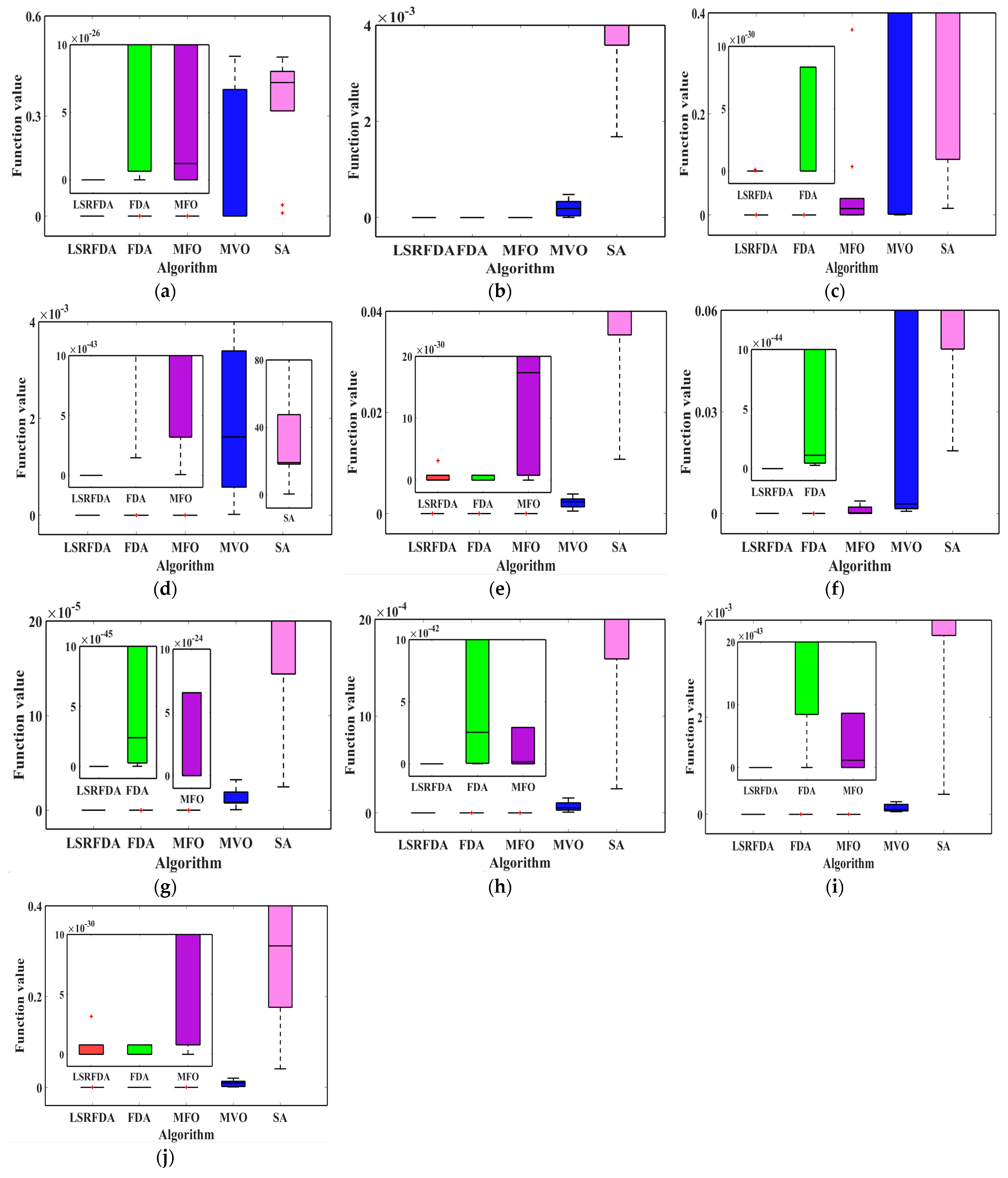
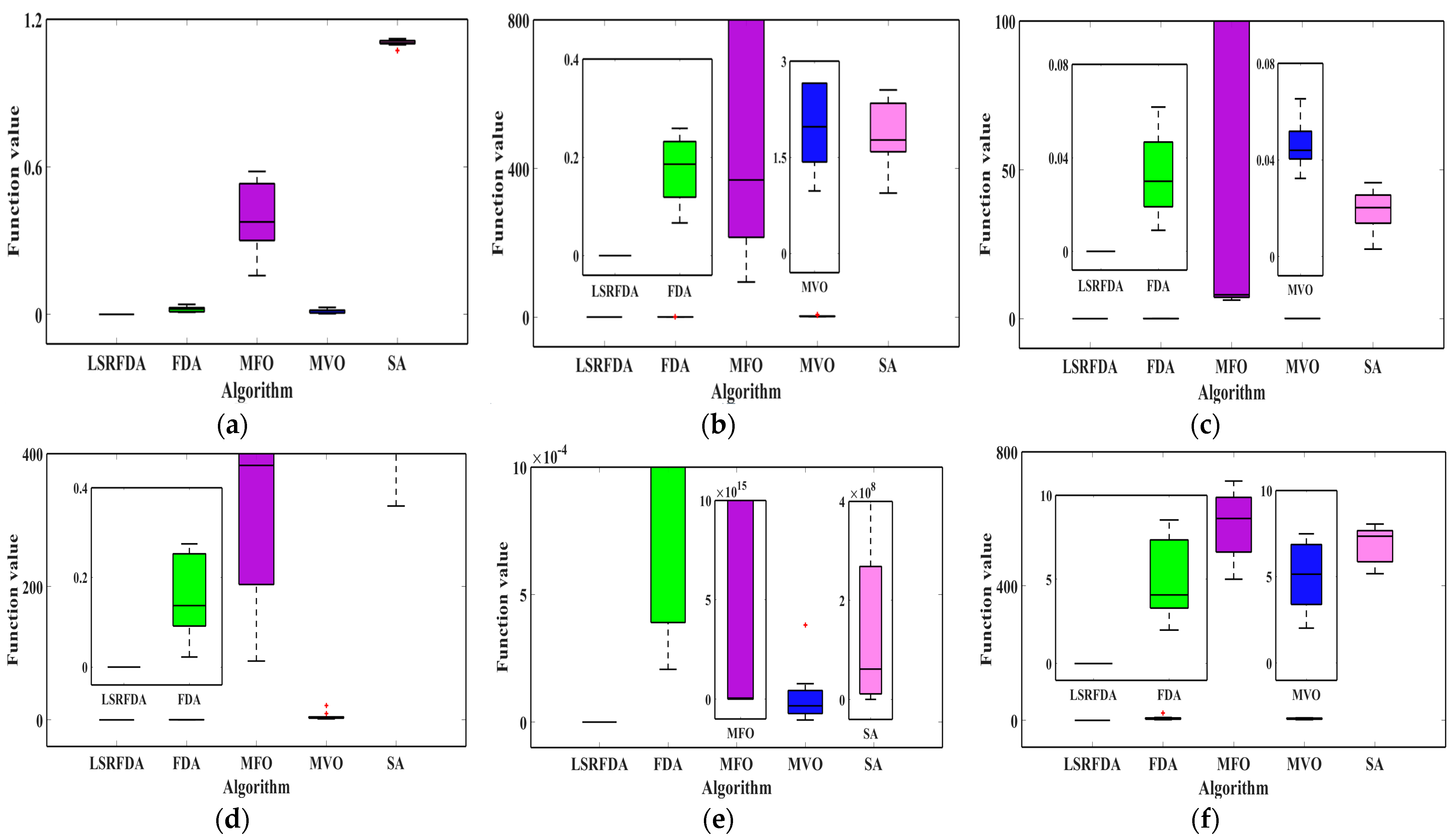
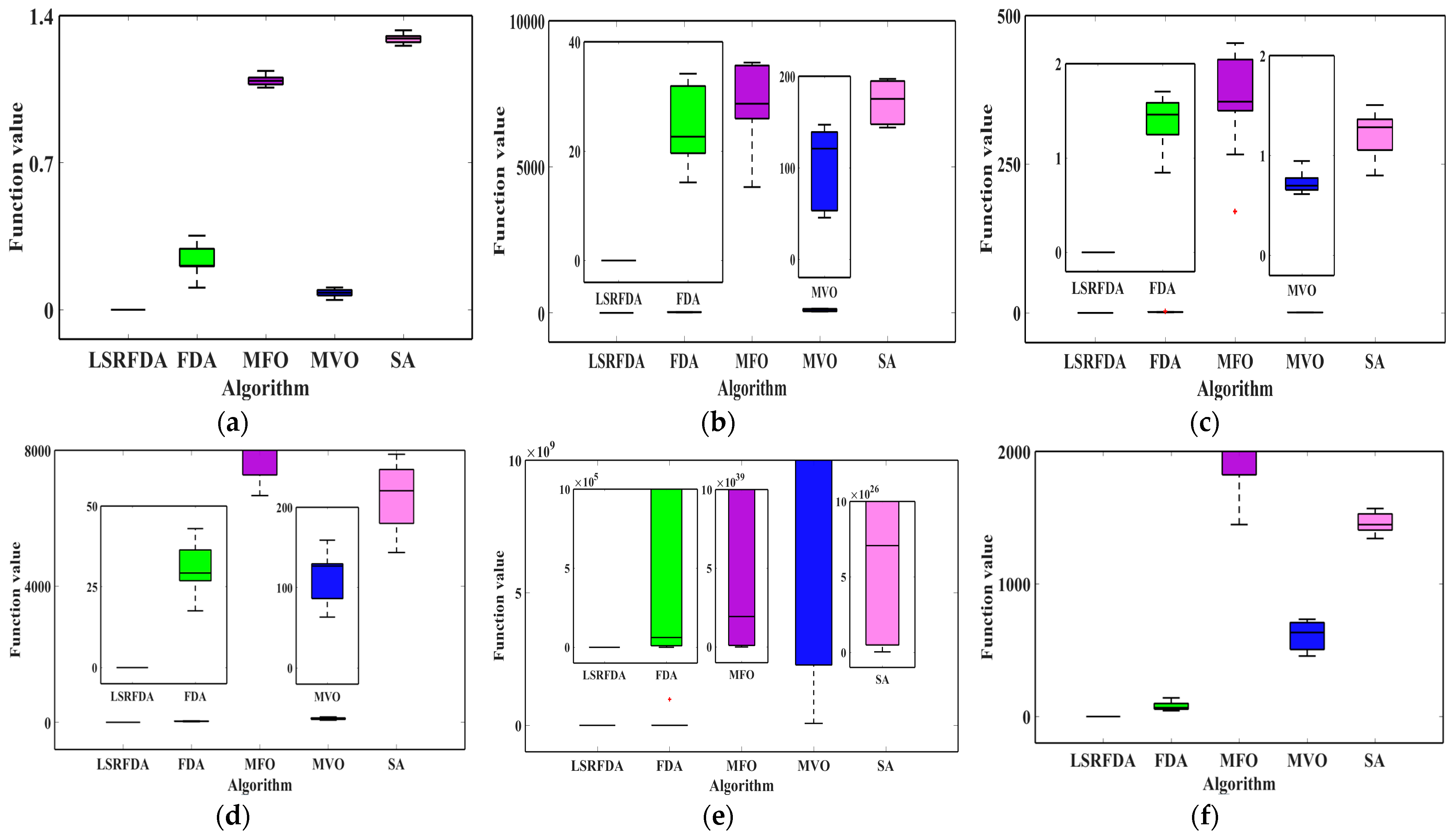
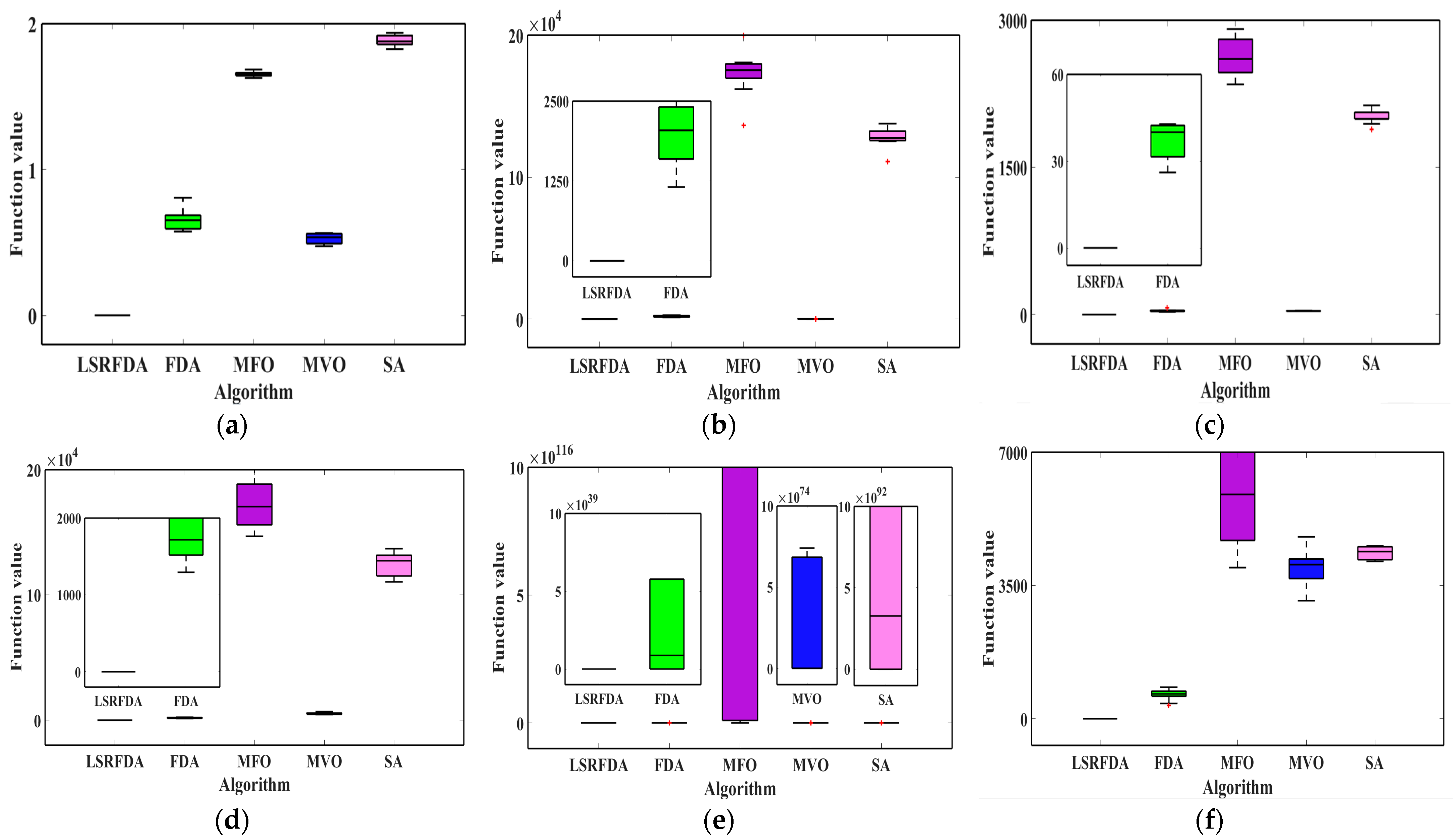
4.6. Box Plot Results Analysis
The box plot is a statistical figure used to show data dispersion information. It is mainly applied to show the distribution characteristics of original data and can also compare their distribution characteristics. In the plot, the box includes the highest value, the lowest value, the median value, the upper and lower quartiles, and the discrete value.
Figure 13,
Figure 14,
Figure 15,
Figure 16 and
Figure 17 are all box plots of different algorithms after 10 independent runs. For most benchmark functions, the LSRFDA has the narrowest box plot, the fewest outliers, the lowest median, and the closest upper and lower quartiles. If the box plot is a straight line, the algorithm has achieved the theoretical optimal value after 10 independent runs. From the above analysis results, it can be seen that the detection step size of individuals in the population affects the final solution accuracy of the algorithm. When the algorithm is in an unknown environment, the population must have a large detection step in the early detection stage to expand the initial searching range. The algorithm should have a small detection step in the late iteration stage for a more accurate and detailed local searching phase. Differently-colored bars represent box plot charts of different algorithms, and red dots represents discrete outlier data in
Figure 13,
Figure 14,
Figure 15,
Figure 16 and
Figure 17.
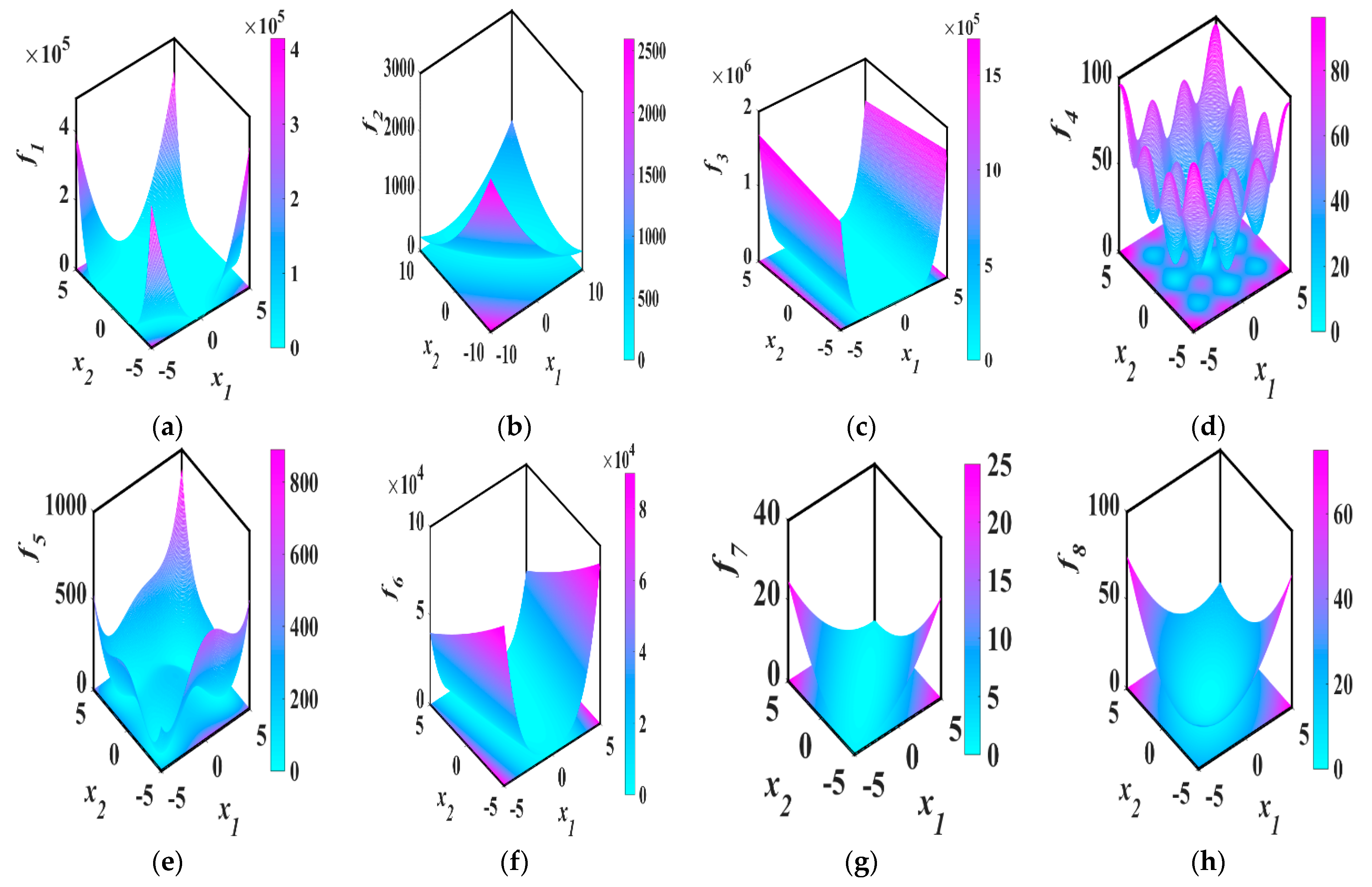
4.7. Search Path Results Analysis
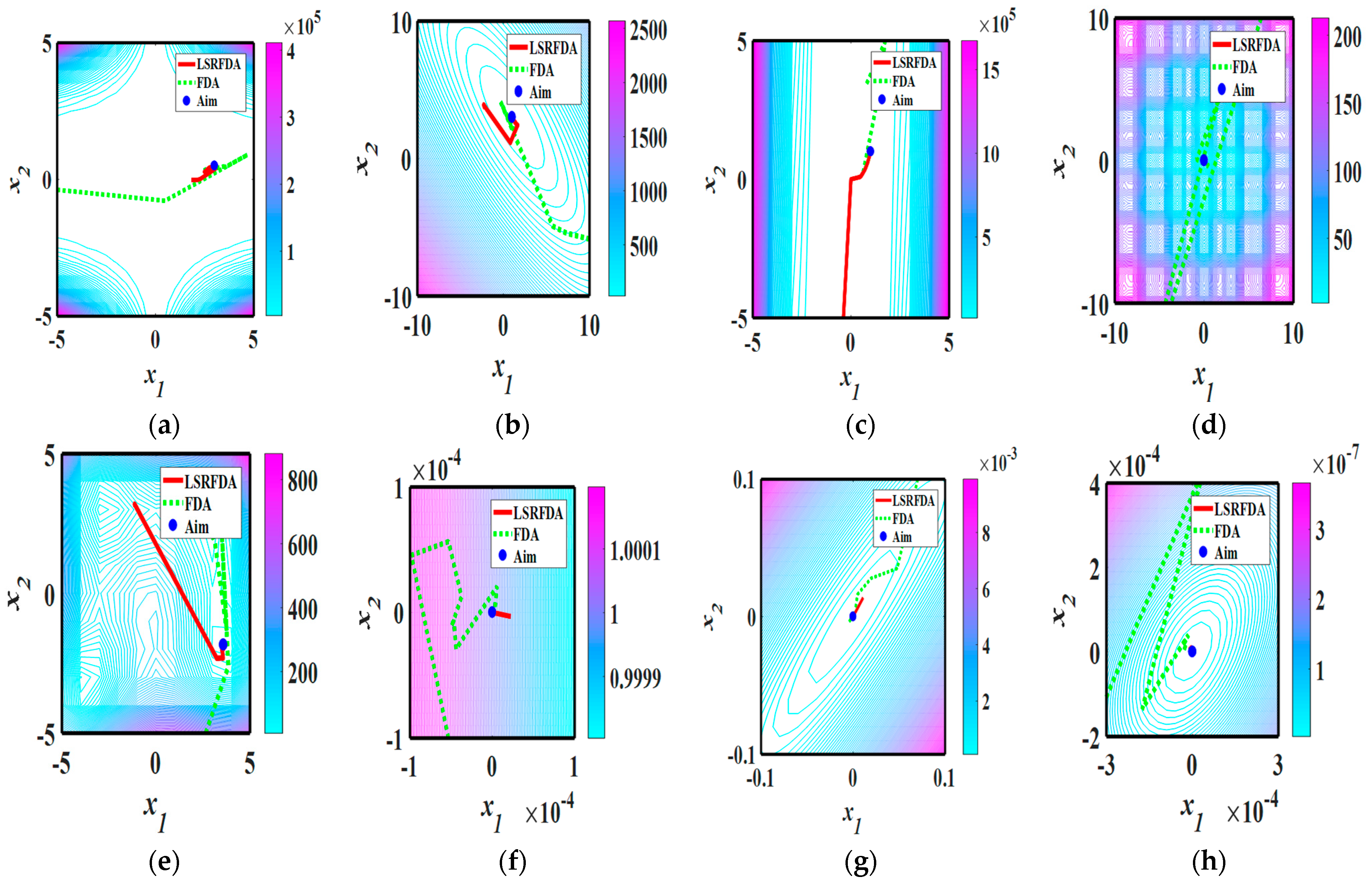
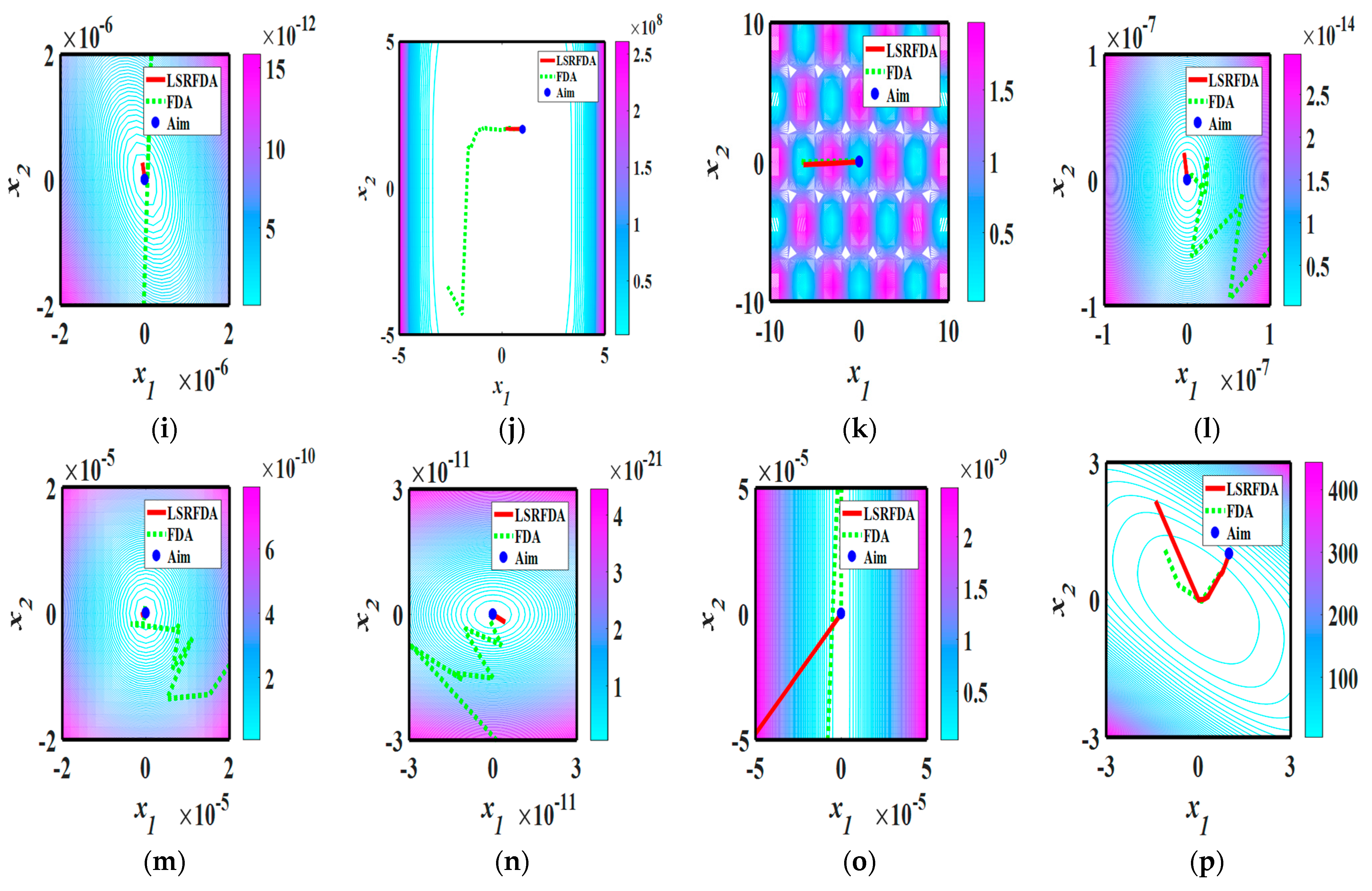
To test the searching speed, the searching efficiency, and the searching accuracy of the LSRFDA, the LSRFDA search path and the original FDA search path are given.
Figure 18 and
Figure 19 show three-dimensional graphs of the benchmark functions and comparison figures of the search path between the LSRFDA and FDA in two-dimensional benchmark functions. The comparison figures are a search path refracted to the two-dimensional plane and a contour map in the two-dimensional plane. The red straight line is the LSRFDA search path. The green dashed line is the FDA search path. The blue origin in the figure is the theoretical optimal position. As can be seen from
Figure 1, the FDA search path is larger than the LSRFDA search path in most search paths. The LSRFDA search path is larger than that of the FDA in
f16. The LSRFDA search path is similar to that of the FDA in
f3,
f11, and
f15. When using the LSRFDA and FDA for search path analysis, there is a significant difference in searching effectiveness. The LSRFDA has significant path advantages, and its planned path length is significantly reduced, indicating significant improvement compared to the basic FDA. After adopting the LSRFDA, during the initial search path, the LSRFDA uses a smaller field of view and fragmented step size to find paths, and can refine and adjust paths to improve their smoothness, which helps to reduce the search path’s length. This is due to the high random jumping characteristic of the LSRFDA, which makes it easy to jump from one region to another region. It can be seen from the figure that the LSRFDA search path cannot easily fall into the local optimal region in the searching process, and its solution accuracy is high, which shows that the LSRFDA can guide and restrict its performance through self-growth strategies to achieve the expected target effect. The search path experiment shows that the proposed algorithm has better solution accuracy and strong searching stability, and its solution quality is higher than that of the basic FDA algorithm. The proposed algorithm can find the optimal solution for the testing function under fewer search paths. Secondly, the proposed algorithm has a high initial global searching ability at the beginning of the search action. At the same time, it can have high solution accuracy and iteration speed.
5. Engineering Optimization Problems
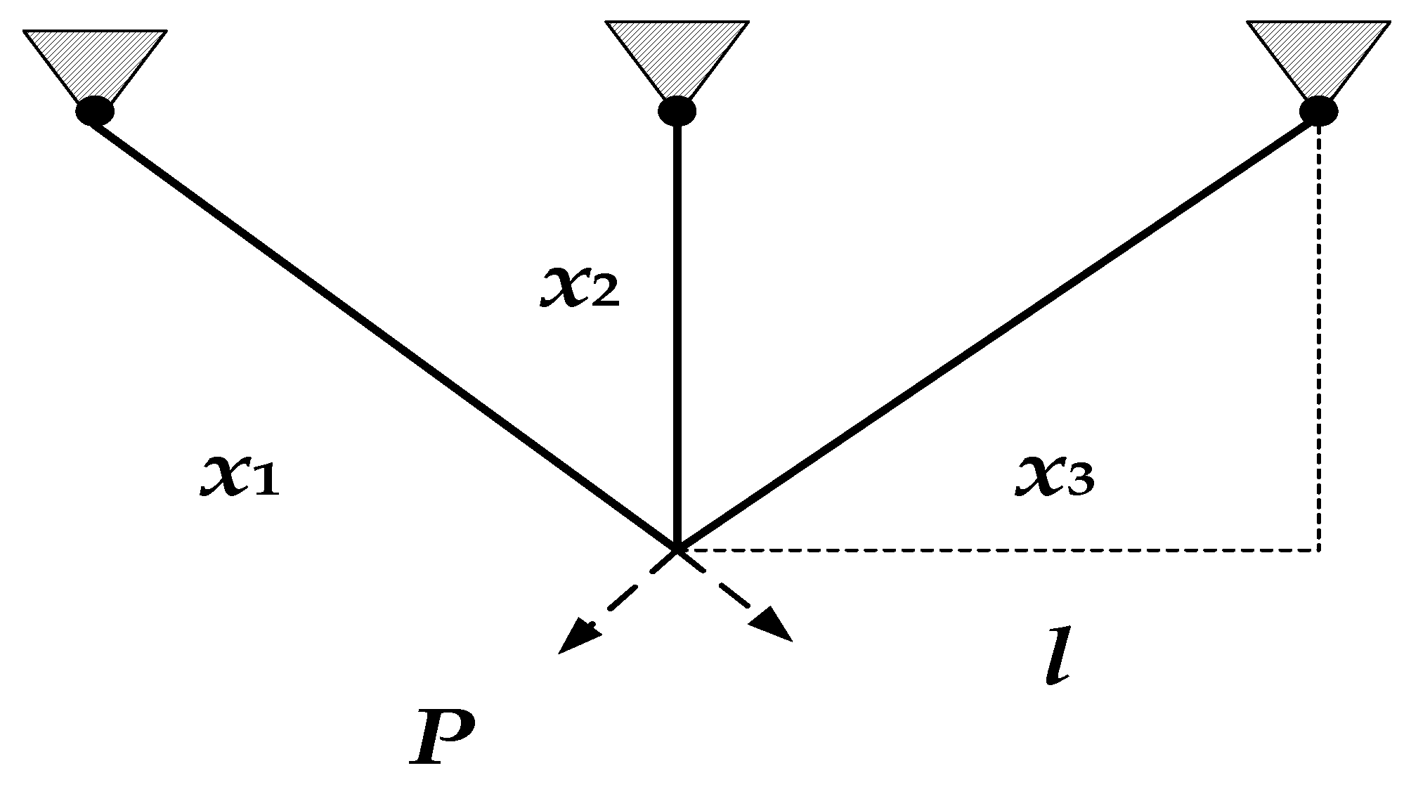
5.1. The Three-Bar Truss Problem
The aim of the three-bar truss problem is to find the optimal value under different constraints including stress, bending, and buckling. This problem has two different decision variables, including the area of the three bars.
Figure 20 shows the structure of the truss and the loads applied to the truss, arrows represent the direction of the force extension. In this figure,
x1 =
x3.
The three-bar truss problem can be formulated as follows:
To solve the three-bar truss problem, the population size, number of neighbors, and number of iterations selected via sensitivity analysis are equal to 25, 3, and 200 in the basic FDA literature. In this paper, all the algorithm parameters were selected based on the basic FDA literature. The LSFDA search results were compared with different algorithms by considering 10 random runs [
28,
29,
30,
31,
32,
33]. The results of the highest and lowest values, the means, and the standard deviation are given in
Table 6. The LSRFDA search result is better than that of the basic FDA. In comparison to this algorithm, the LSRFDA can find the same optimal solution.
5.2. The Tensile/Compression Spring Problem
The tensile/compression spring problem aims is to find the minimum spring weight under different constraints, including pressure, surge frequency, and deflection. In this problem, arrows represent the stretching direction, the three decision variables are the wire diameter (d), the mean spring coil diameter (D), and the number of active spring coils (P), which are denoted by
x1,
x2,
x3.
Figure 21 means the structure of the tensile/compression spring.
The tensile/compression spring problem can be formulated as follows:
To solve the tensile/compression spring problem, the population size, number of neighbors, and number of iterations determined via sensitivity analysis are equal to 50, 1, and 200 in the basic FDA literature. In this paper, all the algorithm parameters were selected based on the basic FDA literature [
28,
29,
30,
31,
32,
33,
34,
35,
36,
37,
38,
39,
40,
41,
42,
43,
44,
45]. The LSRFDA search results were compared with different algorithms by considering 10 random runs. In
Table 7, NO means that the literature does give the value of the algorithm. The LSRFDA search’s highest value, mean value, and standard deviation are higher than those of the FDA’s search result, but the lowest value is lower than that of the FDA search result.
5.3. The Speed Reducer Design Problem
The aim of the speed reducer design problem is to find the minimum cost under different constraints. The objective function can be presented as follows:
To solve the tensile/compression spring problem, the population size, number of neighbors, and number of iterations determined via sensitivity analysis are equal to 50, 1, and 200 in the basic FDA literature. In this paper, all the algorithm parameters were selected based on the basic FDA literature, and the different results are shown in
Table 8. In
Table 8, NO means that the literature does give the value of the algorithm [
28,
29,
30,
31,
32,
33,
34,
35,
36,
37,
38,
39,
40,
41,
42,
43,
44,
45,
46].
The LSRFDA search’s highest value, lowest value, mean value, and standard deviation are higher than those of the FDA search result. Although the test results of the FDA are better than those of the LSRFDA, there is no one algorithm that can solve all engineering problems. Different algorithms have different advantages, and are fit for different object functions.
5.4. The Gear Train Problem
The aim of the gear train design problem is to minimize the cost of the gear ratio in the gear train.
Figure 22 shows the structure of the gear train design problem. The decision variables of the problem are
nA,
nB,
nD, and
nF which are denoted as
x1,
x2,
x3, and
x4, respectively. A, B, D, and F mean centre points. In order to address the discrete variables, all the solutions are rounded to the nearest integer.
The objective function can be presented as follows:
To solve the gear train design problem, the population size, number of neighbors, and number of iterations determined via sensitivity analysis are equal to 50, 1, and 200 in the basic FDA literature. In this paper, all the algorithm parameters were selected based on the basic FDA literature, and the different results are shown in
Table 9. In
Table 9, NO means that the literature does give the value of the algorithm [
33,
34,
35,
36,
37,
38,
39,
40,
41,
42,
43,
44,
45,
46,
47,
48].
The LSRFDA search’s highest value is the same as that of the FDA search result, but the other three values are higher than those of the basic FDA.
6. Discussion
The original FDA literature compared some intelligence algorithms with regard to their functions and engineering optimization problems. The research objective of this paper was to enhance the searching ability, iteration speed, and jumping out power of the optimal local solution in the basic FDA. To discuss this research objective, this paper first tests 16 different functions, and performs numerical calculation results analysis, algorithm sub-sequence calculation results analysis, Wilcoxon rank sum test results analysis, iteration results analysis, box plot results analysis, and searching path results analysis. Then, this paper computes engineering optimization problems, including the three-bar truss problem, the tensile/compression spring problem, the speed reducer design problem, and the gear train problem. To better discuss and analyze the algorithms’ performance, exploratory discussion radar charts are depicted in
Figure 23 to show the ranking of algorithms for each function. If the point of the algorithm in the radar chart is close to the center of the circle, the algorithm has a higher search accuracy. If an algorithm forms a smaller polygon shape in the radar chart, the algorithm has better performance. It can be seen that the LSRFDA surrounds the radar chart center in functions of all dimensions. Additionally, it can be seen that the proposed algorithm ranks first among the other compared algorithms for all the test functions. Regarding the LSRFDA’s limitations and disadvantages, the LSRFDA’s computational complexity is higher than that of the original algorithm, because of the Lévy flight strategy. Because Lévy flight defines the scale-invariant walking model connecting the long gait with the small gait, some engineering optimization problems that require less computationally complex results may generate restrictions. In some search paths, the LSRFDA search path is larger than that of the FDA. In some engineering optimization problems, some testing results of other algorithms are better than those of the proposed method. However, there is no single algorithm that can solve all problems. The LSRFDA has its advantages and disadvantages.
7. Conclusions
In this paper, an LSRFDA algorithm was proposed to solve the optimization problem, which has strong exploitation ability. This proposed algorithm mixed the Lévy flight strategy with the self-renewable method, which can enhance the searching ability, iteration speed, and jumping out power of the optimal local solution of the basic FDA. The combination of the two strategies enables the LSRFDA to effectively follow the correct direction based on the given information, and can increase the robustness and the adaptability of the algorithm. It can generate a uniform distribution in the searching space in the form of a random distribution at the beginning of the algorithm. This paper focused on some difficulties encountered by the FDA in the iterative optimization process and applied the improved FDA to engineering optimization problems. We provide some new methods and ideas for use in the field of engineering optimization problems.
The mathematical testing function experiment results show that the proposed algorithm has better searching ability than the basic FDA algorithm in different benchmark functions, including low-dimensional functions and high-dimensional functions, which shows that the proposed algorithm can enhance the searching ability and iteration speed. Then, this paper selected four engineering optimization problems to further test the performance of the proposed algorithm. For the mathematical testing function experiment, we drew iterative figures, box plots, and search paths to show different performances of the LSRFDA, and the different results show that LSRFDA can jump out of the local optimal solution area and explore a larger solution area in the searching space. In general, the LSFDA has better searchability than the basic FDA algorithm. In the future, the LSRFDA will be used in practical industrial problems. Additionally, we will develop more LSRFDA functions. For future work, we will establish a fusion model based on the FDA and pattern recognition technology, and will deeply integrate the intelligent optimization technology of the hybrid FDA with pattern recognition technology; this could not only achieve the adaptive configuration of model parameters but could also use its superior global convergence performance to further improve the standard training and learning algorithms in pattern recognition models, enhancing their computational accuracy and convergence speed. Then, we will research methods of fault diagnosis based on the FDA, integrate new fault diagnosis methods, and carry out engineering application research based on these FDA fault diagnosis methods, especially for the engineering application of large and complex mechanical systems, expanding the scope for new applications of fault diagnosis.
Author Contributions
Conceptualization, Y.W.; formal analysis, Q.Z.; investigation, Y.W.; resources, Y.W.; writing—original draft preparation, Y.F., S.Z. and D.X.; writing—review and editing, Q.Z.; funding acquisition, Y.W. All authors have read and agreed to the published version of the manuscript.
Funding
This research was funded by basic research business fee projects of provincial undergraduate universities in Heilongjiang Province, grant number: 2022-KYYWF-0144, and the National Natural Science Foundation of China, grant number: 52175502.
Data Availability Statement
The data used to support the findings of this study are available from the corresponding author upon request.
Conflicts of Interest
The authors declare no conflict of interest.
References
- Marseglia, G.; Mesa, J.A.; Ortega, F.A.; Piedra-de-la-Cuadra, R. A heuristic for the deployment of collecting routes for urban recycle stations (eco-points). Socio-Econ. Plan. Sci. 2022, 82, 101222. [Google Scholar] [CrossRef]
- Qin, A.K.; Huang, V.L.; Suganthan, P.N. Differential Evolution Algorithm with Strategy Adaptation for Global Numerical Optimization. IEEE Trans. Evol. Comput. 2009, 13, 398–417. [Google Scholar] [CrossRef]
- Askari, Q.; Saeed, M.; Younas, I. Heap-based optimizer inspired by corporate rank hierarchy for global optimization. Expert Syst. Appl. 2020, 161, 113702. [Google Scholar] [CrossRef]
- Halimu, Y.; Zhou, C.; You, Q.; Sun, J. A Quantum-Behaved Particle Swarm Optimization Algorithm on Riemannian Manifolds. Mathematics 2022, 10, 4168. [Google Scholar] [CrossRef]
- Hou, Y.; Zhang, Y.; Lu, J.; Hou, N.; Yang, D. Application of improved multi-strategy MPA-VMD in pipeline leakage detection. Syst. Sci. Control. Eng. 2023, 11, 2177771. [Google Scholar] [CrossRef]
- Abdollahzadeh, B.; Gharehchopogh, F.S.; Mirjalili, S. African vultures optimization algorithm: A new nature-inspired metaheuristic algorithm for global optimization problems. Comput. Ind. Eng. 2021, 158, 107408. [Google Scholar] [CrossRef]
- You, J.; Jia, H.; Wu, D.; Rao, H.; Wen, C.; Liu, Q.; Abualigah, L. Modified Artificial Gorilla Troop Optimization Algorithm for Solving Constrained Engineering Optimization Problems. Mathematics 2023, 11, 1256. [Google Scholar] [CrossRef]
- Liang, X.; Cai, Z.; Wang, M.; Zhao, X.; Chen, H.; Li, C. Chaotic oppositional sine–cosine method for solving global optimization problems. Eng. Comput. 2020, 38, 1223–1239. [Google Scholar] [CrossRef]
- Wang, G.-G.; Gandomi, A.H.; Alavi, A.H. An effective krill herd algorithm with migration operator in biogeography-based optimization. Appl. Math. Model. 2014, 38, 2454–2462. [Google Scholar] [CrossRef]
- Goldanloo, M.J.; Gharehchopogh, F.S. A hybrid OBL-based firefly algorithm with symbiotic organisms search algorithm for solving continuous optimization problems. J. Supercomput. 2021, 78, 3998–4031. [Google Scholar] [CrossRef]
- Moosavi, S.H.S.; Bardsiri, V.K. Poor and rich optimization algorithm: A new human-based and multi populations algorithm. Eng. Appl. Artif. Intell. 2019, 86, 165–181. [Google Scholar] [CrossRef]
- Zhong, C.; Li, G.; Meng, Z. Beluga whale optimization: A novel nature-inspired metaheuristic algorithm. Knowl.-Based Syst. 2022, 251, 109215. [Google Scholar] [CrossRef]
- Wang, G.-G.; Deb, S.; Cui, Z. Monarch butterfly optimization. Neural Comput. Appl. 2015, 31, 1995–2014. [Google Scholar] [CrossRef]
- Das, B.; Mukherjee, V.; Das, D. Student psychology based optimization algorithm: A new population based optimization algorithm for solving optimization problems. Adv. Eng. Softw. 2020, 146, 102804. [Google Scholar] [CrossRef]
- Chou, J.-S.; Truong, D.-N. A novel metaheuristic optimizer inspired by behavior of jellyfish in ocean. Appl. Math. Comput. 2021, 389, 125535. [Google Scholar] [CrossRef]
- Zervoudakis, K.; Tsafarakis, S. A mayfly optimization algorithm. Comput. Ind. Eng. 2020, 145, 106559. [Google Scholar] [CrossRef]
- Arora, S.; Singh, S. Butterfly optimization algorithm: A novel approach for global optimization. Soft Comput. 2018, 23, 715–734. [Google Scholar] [CrossRef]
- Zainel, Q.M.; Darwish, S.M.; Khorsheed, M.B. Employing Quantum Fruit Fly Optimization Algorithm for Solving Three-Dimensional Chaotic Equations. Mathematics 2022, 10, 4147. [Google Scholar] [CrossRef]
- Cheng, M.-Y.; Prayogo, D. Symbiotic Organisms Search: A new metaheuristic optimization algorithm. Comput. Struct. 2014, 139, 98–112. [Google Scholar] [CrossRef]
- Liu, Z.; Peng, Y. Study on Denoising Method of Vibration Signal Induced by Tunnel Portal Blasting Based on WOA-VMD Algorithm. Appl. Sci. 2023, 13, 3322. [Google Scholar] [CrossRef]
- Karami, H.; Anaraki, M.V.; Farzin, S.; Mirjalili, S. Flow Direction Algorithm (FDA): A Novel Optimization Approach for Solving Optimization Problems. Comput. Ind. Eng. 2021, 156, 107224. [Google Scholar] [CrossRef]
- Abualigah, L.; Almotairi, K.H.; Elaziz, M.A.; Shehab, M.; Altalhi, M. Enhanced Flow Direction Arithmetic Optimization Algorithm for mathematical optimization problems with applications of data clustering. Eng. Anal. Bound. Elem. 2022, 138, 13–29. [Google Scholar] [CrossRef]
- Jourdain, B.; Méléard, S.; Woyczynski, W.A. Lévy flights in evolutionary ecology. J. Math. Biol. 2012, 65, 677–707. [Google Scholar] [CrossRef] [PubMed]
- Pavlyukevich, I. Lévy flights, non-local search and simulated annealing. J. Comput. Phys. 2007, 226, 1830–1844. [Google Scholar] [CrossRef]
- Mirjalili, S. Moth-flame optimization algorithm: A novel nature-inspired heuristic paradigm. Knowl.-Based Syst. 2015, 89, 228–249. [Google Scholar] [CrossRef]
- Mirjalili, S.; Mirjalili, S.M.; Hatamlou, A. Multi-Verse Optimizer: A nature-inspired algorithm for global optimization. Neural Comput. Appl. 2016, 27, 495–513. [Google Scholar] [CrossRef]
- Osman, I.H. Metastrategy simulated annealing and tabu search algorithms for the vehicle routing problem. Ann. Oper. Res 1993, 41, 421–451. [Google Scholar] [CrossRef]
- Ray, T.; Liew, K.M. Society and civilization: An optimization algorithm based on the simulation of social behavior. IEEE Trans. Evol. Comput. 2003, 7, 386–396. [Google Scholar] [CrossRef]
- Liu, H.; Cai, Z.; Wang, Y. Hybridizing particle swarm optimization with differential evolution for constrained numerical and engineering optimization. Appl. Soft. Comput. 2010, 10, 629–640. [Google Scholar] [CrossRef]
- Zhang, M.; Luo, W.; Wang, X. Differential evolution with dynamic stochastic selection for constrained optimization. Inf. Sci. 2008, 178, 3043–3074. [Google Scholar] [CrossRef]
- Wang, Y.; Cai, Z.; Zhou, Y.; Fan, Z. Constrained optimization based on hybrid evolutionary algorithm and adaptive constraint-handling technique. Struct. Multidiscip. Optim. 2008, 37, 395–413. [Google Scholar] [CrossRef]
- Eskandar, H.; Sadollah, A.; Bahreininejad, A.; Hamdi, M. Water cycle algorithm—A novel metaheuristic optimization method for solving constrained engineering optimization problems. Comput. Struct. 2012, 110–111, 151–166. [Google Scholar] [CrossRef]
- Sadollah, A.; Bahreininejad, A.; Eskandar, H.; Hamdi, M. Mine blast algorithm: A new population based algorithm for solving constrained engineering optimization problems. Appl. Soft. Comput. 2013, 13, 2592–2612. [Google Scholar] [CrossRef]
- Coello Coello, C.A. Use of a self-adaptive penalty approach for engineering optimization problems. Comput. Ind. 2000, 41, 113–127. [Google Scholar] [CrossRef]
- Coello Coello, C.A.; Mezura Montes, E. Constraint-handling in genetic algorithms through the use of dominance-based tournament selection. Adv. Eng. Inf. 2002, 16, 193–203. [Google Scholar] [CrossRef]
- He, Q.; Wang, L. A hybrid particle swarm optimization with a feasibility-based rule for constrained optimization. Appl. Math. Comput. 2007, 186, 1407–1422. [Google Scholar] [CrossRef]
- Zahara, E.; Kao, Y.-T. Hybrid Nelder–Mead simplex search and particle swarm optimization for constrained engineering design problems. Expert Syst. Appl. 2009, 36, 3880–3886. [Google Scholar] [CrossRef]
- Coelho, L.d.S. Gaussian quantum-behaved particle swarm optimization approaches for constrained engineering design problems. Expert Syst. Appl. 2010, 37, 1676–1683. [Google Scholar] [CrossRef]
- Wang, L.; Li, L.-p. An effective differential evolution with level comparison for constrained engineering design. Struct. Multidiscip. Optim. 2009, 41, 947–963. [Google Scholar] [CrossRef]
- Parsopoulos, K.E.; Vrahatis, M.N. Unified Particle Swarm Optimization for Solving Constrained Engineering Optimization Problems. In Proceedings of the Advances in Natural Computation, Changsha, China, 27–29 August 2005; pp. 582–591. Available online: https://link.springer.com/chapter/10.1007/11539902_71 (accessed on 29 August 2005).
- Huang, F.-z.; Wang, L.; He, Q. An effective co-evolutionary differential evolution for constrained optimization. Appl. Math. Comput. 2007, 186, 340–356. [Google Scholar] [CrossRef]
- Mezura-Montes, E.; Coello, C.A.C. Useful Infeasible Solutions in Engineering Optimization with Evolutionary Algorithms. In Proceedings of the MICAI 2005: Advances in Artificial Intelligence, Monterrey, Mexico, 14–18 November 2005; pp. 652–662. Available online: https://link.springer.com/chapter/10.1007/11579427_66 (accessed on 18 November 2005).
- Akay, B.; Karaboga, D. Artificial bee colony algorithm for large-scale problems and engineering design optimization. J. Intell. Manuf. 2010, 23, 1001–1014. [Google Scholar] [CrossRef]
- Rao, R.V.; Savsani, V.J.; Vakharia, D.P. Teaching–learning-based optimization: A novel method for constrained mechanical design optimization problems. Comput.-Aided Des. 2011, 43, 303–315. [Google Scholar] [CrossRef]
- Askarzadeh, A. A novel metaheuristic method for solving constrained engineering optimization problems: Crow search algorithm. Comput. Struct. 2016, 169, 1–12. [Google Scholar] [CrossRef]
- Zhao, W.; Zhang, Z.; Wang, L. Manta ray foraging optimization: An effective bio-inspired optimizer for engineering applications. Eng. Appl. Artif. Intell. 2020, 87, 103300. [Google Scholar] [CrossRef]
- Gandomi, A.H.; Yang, X.-S.; Alavi, A.H. Cuckoo search algorithm: A metaheuristic approach to solve structural optimization problems. Eng. Comput. 2011, 29, 17–35. [Google Scholar] [CrossRef]
- Mirjalili, S. The Ant Lion Optimizer. Adv. Eng. Softw. 2015, 83, 80–98. [Google Scholar] [CrossRef]
Figure 1.
Lévy flight path. (a) Two dimensional Lévy flight path; (b) Three dimensional Lévy flight path.
Figure 1.
Lévy flight path. (a) Two dimensional Lévy flight path; (b) Three dimensional Lévy flight path.
Figure 2.
The flowchart for LSRFDA.
Figure 2.
The flowchart for LSRFDA.
Figure 3.
Sub-sequence run radar charts for low−dimensional functions. (a) f1.; (b) f2; (c) f3; (d) f4; (e) f5; (f) f6; (g) f7; (h) f8; (i) f9; (j) f10.
Figure 3.
Sub-sequence run radar charts for low−dimensional functions. (a) f1.; (b) f2; (c) f3; (d) f4; (e) f5; (f) f6; (g) f7; (h) f8; (i) f9; (j) f10.
Figure 4.
Sub-sequence run radar charts for variable–dimensional functions (D = 2). (a) f11(D=2); (b) f12(D=2); (c) f13(D=2); (d) f14(D=2); (e) f15(D=2); (f) f16(D=2).
Figure 4.
Sub-sequence run radar charts for variable–dimensional functions (D = 2). (a) f11(D=2); (b) f12(D=2); (c) f13(D=2); (d) f14(D=2); (e) f15(D=2); (f) f16(D=2).
Figure 5.
Sub-sequence run radar charts for variable–dimensional functions (D = 30). (a) f11(D=30); (b) f12(D=30); (c) f13(D=30); (d) f14(D=30); (e) f15(D=30); (f) f16(D=30).
Figure 5.
Sub-sequence run radar charts for variable–dimensional functions (D = 30). (a) f11(D=30); (b) f12(D=30); (c) f13(D=30); (d) f14(D=30); (e) f15(D=30); (f) f16(D=30).
Figure 6.
Sub-sequence run radar charts for variable–dimensional functions (D = 60). (a) f11(D=60); (b) f12(D=60); (c) f13(D=60); (d) f14(D=60); (e) f15(D=60); (f) f16(D=60).
Figure 6.
Sub-sequence run radar charts for variable–dimensional functions (D = 60). (a) f11(D=60); (b) f12(D=60); (c) f13(D=60); (d) f14(D=60); (e) f15(D=60); (f) f16(D=60).
Figure 7.
Sub-sequence run radar charts for variable–dimensional functions (D = 150). (a) f11(D=150); (b) f12(D=150); (c) f13(D=150); (d) f14(D=150); (e) f15(D=150); (f) f16(D=150).
Figure 7.
Sub-sequence run radar charts for variable–dimensional functions (D = 150). (a) f11(D=150); (b) f12(D=150); (c) f13(D=150); (d) f14(D=150); (e) f15(D=150); (f) f16(D=150).
Figure 8.
Convergence curves for low−dimensional functions. (a) f1.; (b) f2; (c) f3; (d) f4; (e) f5; (f) f6; (g) f7; (h) f8; (i) f9; (j) f10.
Figure 8.
Convergence curves for low−dimensional functions. (a) f1.; (b) f2; (c) f3; (d) f4; (e) f5; (f) f6; (g) f7; (h) f8; (i) f9; (j) f10.
Figure 9.
Convergence curves for variable–dimensional functions (D = 2). (a) f11(D=2); (b) f12(D=2); (c) f13(D=2); (d) f14(D=2); (e) f15(D=2); (f) f16(D=2).
Figure 9.
Convergence curves for variable–dimensional functions (D = 2). (a) f11(D=2); (b) f12(D=2); (c) f13(D=2); (d) f14(D=2); (e) f15(D=2); (f) f16(D=2).
Figure 10.
Convergence curves for variable–dimensional functions (D = 30). (a) f11(D=30); (b) f12(D=30); (c) f13(D=30); (d) f14(D=30); (e) f15(D=30); (f) f16(D=30).
Figure 10.
Convergence curves for variable–dimensional functions (D = 30). (a) f11(D=30); (b) f12(D=30); (c) f13(D=30); (d) f14(D=30); (e) f15(D=30); (f) f16(D=30).
Figure 11.
Convergence curves for variable–dimensional functions (D = 60). (a) f11(D=60); (b) f12(D=60); (c) f13(D=60); (d) f14(D=60); (e) f15(D=60); (f) f16(D=60).
Figure 11.
Convergence curves for variable–dimensional functions (D = 60). (a) f11(D=60); (b) f12(D=60); (c) f13(D=60); (d) f14(D=60); (e) f15(D=60); (f) f16(D=60).
Figure 12.
Convergence curves for variable–dimensional functions (D = 150). (a) f11(D=150); (b) f12(D=150); (c) f13(D=150); (d) f14(D=150); (e) f15(D=150); (f) f16(D=150).
Figure 12.
Convergence curves for variable–dimensional functions (D = 150). (a) f11(D=150); (b) f12(D=150); (c) f13(D=150); (d) f14(D=150); (e) f15(D=150); (f) f16(D=150).
Figure 13.
Box plot charts for low dimension functions. (a) f1.; (b) f2; (c) f3; (d) f4; (e) f5; (f) f6; (g) f7; (h) f8; (i) f9; (j) f10.
Figure 13.
Box plot charts for low dimension functions. (a) f1.; (b) f2; (c) f3; (d) f4; (e) f5; (f) f6; (g) f7; (h) f8; (i) f9; (j) f10.
Figure 14.
Box plot charts for variable–dimensional functions (D = 2). (a) f11(D=2); (b) f12(D=2); (c) f13(D=2); (d) f14(D=2); (e) f15(D=2); (f) f16(D=2).
Figure 14.
Box plot charts for variable–dimensional functions (D = 2). (a) f11(D=2); (b) f12(D=2); (c) f13(D=2); (d) f14(D=2); (e) f15(D=2); (f) f16(D=2).
Figure 15.
Box plot charts for variable–dimensional functions (D = 30). (a) f11(D=30); (b) f12(D=30); (c) f13(D=30); (d) f14(D=30); (e) f15(D=30); (f) f16(D=30).
Figure 15.
Box plot charts for variable–dimensional functions (D = 30). (a) f11(D=30); (b) f12(D=30); (c) f13(D=30); (d) f14(D=30); (e) f15(D=30); (f) f16(D=30).
Figure 16.
Box plot charts for variable–dimensional functions (D = 60). (a) f11(D=60); (b) f12(D=60); (c) f13(D=60); (d) f14(D=60); (e) f15(D=60); (f) f16(D=60).
Figure 16.
Box plot charts for variable–dimensional functions (D = 60). (a) f11(D=60); (b) f12(D=60); (c) f13(D=60); (d) f14(D=60); (e) f15(D=60); (f) f16(D=60).
Figure 17.
Box plot charts for variable–dimensional functions (D = 150). (a) f11(D=150); (b) f12(D=150); (c) f13(D=150); (d) f14(D=150); (e) f15(D=150); (f) f16(D=150).
Figure 17.
Box plot charts for variable–dimensional functions (D = 150). (a) f11(D=150); (b) f12(D=150); (c) f13(D=150); (d) f14(D=150); (e) f15(D=150); (f) f16(D=150).
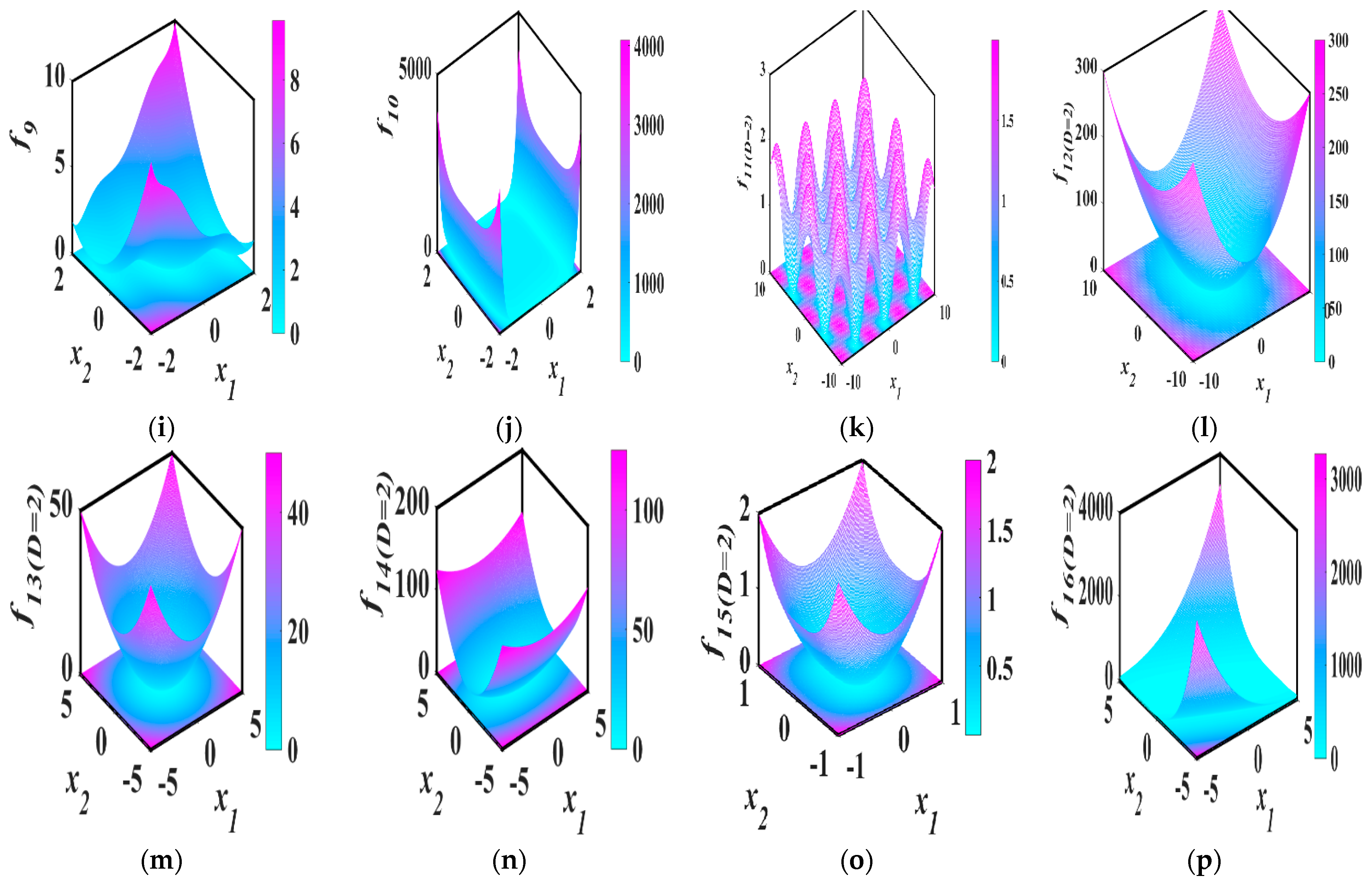
Figure 18.
Three−dimensional graphs of benchmark functions. (a) f1.; (b) f2; (c) f3; (d) f4; (e) f5; (f) f6; (g) f7; (h) f8; (i) f9; (j) f10; (k) f11(D=2); (l) f12(D=2); (m) f13(D=2); (n) f14(D=2); (o) f15(D=2); (p) f16(D=2).
Figure 18.
Three−dimensional graphs of benchmark functions. (a) f1.; (b) f2; (c) f3; (d) f4; (e) f5; (f) f6; (g) f7; (h) f8; (i) f9; (j) f10; (k) f11(D=2); (l) f12(D=2); (m) f13(D=2); (n) f14(D=2); (o) f15(D=2); (p) f16(D=2).
Figure 19.
Algorithm search paths. (a) f1.; (b) f2; (c) f3; (d) f4; (e) f5; (f) f6; (g) f7; (h) f8; (i) f9; (j) f10; (k) f11(D=2); (l) f12(D=2); (m) f13(D=2); (n) f14(D=2); (o) f15(D=2); (p) f16(D=2).
Figure 19.
Algorithm search paths. (a) f1.; (b) f2; (c) f3; (d) f4; (e) f5; (f) f6; (g) f7; (h) f8; (i) f9; (j) f10; (k) f11(D=2); (l) f12(D=2); (m) f13(D=2); (n) f14(D=2); (o) f15(D=2); (p) f16(D=2).
Figure 20.
Schematic of the three-bar truss problem.
Figure 20.
Schematic of the three-bar truss problem.
Figure 21.
Schematic of the tensile/compression spring problem.
Figure 21.
Schematic of the tensile/compression spring problem.
Figure 22.
Schematic of the gear train problem.
Figure 22.
Schematic of the gear train problem.
Figure 23.
Algorithm ranking. (a) Algorithm ranking in two-dimensional functions; (b) Algorithm ranking in 30-dimensional functions; (c) Algorithm ranking in 60-dimensional functions; (d) Algorithm ranking in 150-dimensional functions.
Figure 23.
Algorithm ranking. (a) Algorithm ranking in two-dimensional functions; (b) Algorithm ranking in 30-dimensional functions; (c) Algorithm ranking in 60-dimensional functions; (d) Algorithm ranking in 150-dimensional functions.
Table 1.
Basic information on benchmark functions.
Table 1.
Basic information on benchmark functions.
| Name | Function | D | Range | fmin |
|---|
| Beale | f1(x) = (1.5 − x1 + x1x2)2 + (2.25 − x1 + x1)2
+ (2.625 − x1+ x1)2 | 2 | [−100, 100] | 0 |
| Booth | f2(x) = (x1 + 2x2 − 7)2 + (2x1 + x2 − 5)2 | 2 | [−100, 100] | 0 |
| Cube | f3(x) = 100(x2 − )2 + (1 − x1)2 | 2 | [−100, 100] | 0 |
| Egg Crate | f4(x) = + + 25(sin2(x1) + sin2(x2)) | 2 | [−100, 100] | 0 |
| Himmelblau | f5(x) = ( + x2 − 11)2 + (x1 + − 7)2 | 2 | [−100, 100] | 0 |
| Leon | f6(x) = 100(x2 − )2 + (1 − x1)2 | 2 | [−100, 100] | 0 |
| Matyas | f7(x) = 0.26( + ) −0.48x1x2 | 2 | [−100, 100] | 0 |
| RotatedEllipse02 | f8(x) = − x1x2 + | 2 | [−100, 100] | 0 |
| Three-Hump Camel | f9(x) = 2 − 1.05 + /6 + x1x2 + | 2 | [−100, 100] | 0 |
| Wayburn Seader01 | f10(x) = ( + − 17)2 + (2x1 + x2 − 4)2 | 2 | [−100, 100] | 0 |
| Griewank | | 2/30/60/150 | [−10, 10] | 0 |
| Rotated Hyper-Ellipsoid | | 2/30/60/150 | [−10, 10] | 0 |
| Sphere | | 2/30/60/150 | [−10, 10] | 0 |
| Sum Squares | | 2/30/60/150 | [−10, 10] | 0 |
| Sum of Different Powers | | 2/30/60/150 | [−10, 10] | 0 |
| Zakharov | | 2/30/60/150 | [−10, 10] | 0 |
Table 2.
Basic information on benchmark functions.
Table 2.
Basic information on benchmark functions.
| Algorithm | Key Feature Parameter | Max_Iter | N |
|---|
| LSRFDA | Lévy flight length: Sl. Power law index: β. | 200 | 50 |
| FDA | Random vector: . Random position: Xrand. Random number: rand. |
| MFO | Random number: t. Constant: b. |
| MVO | Random number: r1, r2, r3, r4. Coefficient number: TDR, WEP. Exploitation accuracy: p. Minimum and maximum numbers: min, max. |
| SA | Initial temperature: t0. Attenuation factor: k. |
Table 3.
Comparison of results for two-dimensional functions.
Table 3.
Comparison of results for two-dimensional functions.
| Function | Metric | LSRFDA | FDA | MFO | MVO | SA |
|---|
| f1 | Min | 0 | 0 | 0 | 2.6946 × 10⁻⁵ | 0.0096 |
| Max | 0 | 7.3704 × 10⁻⁷ | 1.4092 × 10⁻¹⁶ | 0.4792 | 0.4769 |
| Ave | 0 | 7.3704 × 10⁻⁸ | 1.4092 × 10⁻¹⁷ | 0.1294 | 0.3301 |
| f2 | Min | 0 | 0 | 0 | 2.2357 × 10⁻⁶ | 0.0017 |
| Max | 0 | 0 | 0 | 0.0005 | 0.0174 |
| Ave | 0 | 0 | 0 | 0.0002 | 0.0069 |
| f3 | Min | 0 | 0 | 9.5342 × 10⁻⁵ | 0.0003 | 0.0132 |
| Max | 1.1093 × 10⁻³¹ | 1.6575 × 10⁻¹⁶ | 0.3662 | 8.4851 | 4.4566 |
| Ave | 1.6024 × 10⁻³² | 1.6575 × 10⁻¹⁷ | 0.0538 | 1.8117 | 1.3225 |
| f4 | Min | 0 | 1.4725 × 10−43 | 6.9502 × 10−45 | 1.8314 × 10⁻⁵ | 0.3767 |
| Max | 0 | 1.9320 × 10⁻³⁴ | 4.0349 × 10−38 | 0.0066 | 85.3771 |
| Ave | 0 | 3.6561 × 10⁻³⁵ | 4.0399 × 10−39 | 0.0023 | 33.2411 |
| f5 | Min | 0 | 0 | 0 | 0.0005 | 0.0108 |
| Max | 3.1554 × 10⁻³⁰ | 8.8920 × 10⁻²⁶ | 9.3983 × 10⁻²⁶ | 0.0039 | 0.3501 |
| Ave | 7.0998 × 10⁻³¹ | 8.8922 × 10⁻²⁷ | 1.3632 × 10⁻²⁶ | 0.0021 | 0.0934 |
| f6 | Min | 0 | 2.7794 × 10−45 | 1.4127 × 10⁻⁹ | 0.0006 | 0.0185 |
| Max | 0 | 1.3670 × 10−42 | 2.6005 | 38.6167 | 0.3772 |
| Ave | 0 | 2.6631 × 10−43 | 0.2607 | 7.7896 | 0.1339 |
| f7 | Min | 0 | 1.2152 × 10−47 | 1.9600 × 10−39 | 4.9588 × 10⁻⁷ | 2.4612 × 10⁻⁵ |
| Max | 0 | 1.7254 × 10−40 | 1.8402 × 10⁻¹⁸ | 3.2146 × 10⁻⁵ | 0.0011 |
| Ave | 0 | 1.7603 × 10−41 | 2.3675 × 10⁻¹⁹ | 1.2289 × 10⁻⁵ | 0.0005 |
| f8 | Min | 0 | 8.3261 × 10−45 | 4.0001 × 10−47 | 7.4928 × 10⁻⁶ | 0.0002 |
| Max | 0 | 6.6272 × 10−37 | 2.2733 × 10−39 | 0.0001 | 0.0054 |
| Ave | 0 | 6.8364 × 10−38 | 2.3244 × 10−40 | 6.6311 × 10⁻⁵ | 0.002970385 |
| f9 | Min | 0 | 7.3650 × 10−46 | 4.5065 × 10−47 | 5.4736 × 10⁻⁵ | 0.0004 |
| Max | 0 | 1.6197 × 10−38 | 4.4818 × 10−42 | 0.0003 | 0.3006 |
| Ave | 0 | 1.9097 × 10−39 | 8.7414 × 10−43 | 0.0001 | 0.0416 |
| f10 | Min | 0 | 0 | 0 | 0.0009 | 0.0408 |
| Max | 1.3411 × 10⁻²⁹ | 7.8886 × 10⁻³¹ | 2.6225 × 10⁻²¹ | 0.0202 | 4.5708 |
| Ave | 1.9722 × 10⁻³⁰ | 3.1554 × 10⁻³¹ | 3.5098 × 10⁻²² | 0.0086 | 0.7425 |
| f11(D=2) | Min | 0 | 0 | 0 | 7.2263 × 10⁻⁷ | 0.0006 |
| Max | 0 | 3.6366 × 10⁻¹¹ | 0.0099 | 0.0296 | 0.0050 |
| Ave | 0 | 5.5746 × 10⁻¹² | 0.0064 | 0.0150 | 0.0019 |
| f12(D=2) | Min | 0 | 2.4682 × 10−41 | 2.1456 × 10−49 | 8.3964 × 10⁻⁸ | 4.3981 × 10⁻⁵ |
| Max | 0 | 6.8949 × 10⁻³⁵ | 3.3578 × 10−44 | 3.8819 × 10⁻⁶ | 0.0011 |
| Ave | 0 | 6.9221 × 10−36 | 3.4030 × 10−45 | 1.3765 × 10⁻⁶ | 0.0005 |
| f13(D=2) | Min | 0 | 1.3668 × 10−39 | 2.1177 × 10−49 | 2.0121 × 10⁻⁷ | 2.5717 × 10⁻⁵ |
| Max | 0 | 4.4792 × 10−36 | 1.2284 × 10−44 | 2.0760 × 10⁻⁶ | 0.0005 |
| Ave | 0 | 9.0174 × 10−37 | 2.8524 × 10−45 | 1.3137 × 10⁻⁶ | 0.0002 |
| f14(D=2) | Min | 0 | 3.3512 × 10−41 | 4.8850 × 10−53 | 4.4806 × 10⁻⁸ | 2.2747 × 10⁻⁷ |
| Max | 0 | 3.6176 × 10⁻³⁵ | 2.8707 × 10−45 | 4.4295 × 10⁻⁶ | 0.0008 |
| Ave | 0 | 6.0365 × 10−36 | 3.0331 × 10−46 | 1.1654 × 10⁻⁶ | 0.0003 |
| f15(D=2) | Min | 0 | 9.3840 × 10−61 | 4.2891 × 10−58 | 7.1028 × 10⁻¹⁰ | 1.4138 × 10⁻⁶ |
| Max | 0 | 2.2466 × 10−49 | 1.2316 × 10−52 | 1.4890 × 10⁻⁷ | 0.0001 |
| Ave | 0 | 2.2469 × 10−50 | 1.3073 × 10−53 | 2.7849 × 10⁻⁸ | 2.8356 × 10⁻⁵ |
| f16(D=2) | Min | 0 | 0 | 1.5809 × 10−49 | 1.3379 × 10⁻⁸ | 1.5844 × 10⁻⁵ |
| Max | 0 | 1.0366 × 10⁻²⁹ | 8.0164 × 10−45 | 4.5850 × 10⁻⁶ | 0.0004 |
| Ave | 0 | 1.0366 × 10⁻³⁰ | 1.9613 × 10−45 | 1.4956 × 10⁻⁶ | 0.0002 |
Table 4.
Comparison of results for 30-, 60-, and 150-dimensional functions.
Table 4.
Comparison of results for 30-, 60-, and 150-dimensional functions.
| Function | Metric | LSRFDA | FDA | MFO | MVO | SA |
|---|
| f11(D=30) | Min | 0 | 0.0090 | 0.1578 | 0.0031 | 1.0736 |
| Max | 0 | 0.0407 | 0.5812 | 0.0283 | 1.1207 |
| Ave | 0 | 0.0215 | 0.3867 | 0.0142 | 1.1042 |
| f12(D=30) | Min | 0 | 0.0664 | 94.4089 | 0.9747 | 3.3371 × 10² |
| Max | 0 | 0.5313 | 3.2261 × 10³ | 6.0745 | 6.1136 × 10² |
| Ave | 0 | 0.2051 | 7.9935 × 10² | 2.4544 | 4.8891 × 10² |
| f13(D=30) | Min | 0 | 0.0090 | 6.24125 | 0.0323 | 23.3850 |
| Max | 0 | 0.0617 | 1.1021 × 10² | 0.0653 | 45.6998 |
| Ave | 0 | 0.0321 | 37.2880 | 0.0459 | 35.8305 |
| f14(D=30) | Min | 0 | 0.0225 | 88.5232 | 1.4932 | 3.2128 × 10² |
| Max | 0 | 0.2746 | 7.0043 × 10² | 21.2344 | 5.6142 × 10² |
| Ave | 0 | 0.1501 | 3.5094 × 10² | 5.5779 | 4.7041 × 10² |
| f15(D=30) | Min | 0 | 0.0002 | 1.6312 × 10¹⁰ | 8.3515 × 10⁻⁶ | 5.3366 × 10⁵ |
| Max | 0 | 0.0143 | 1.0000 × 10¹⁹ | 0.0004 | 1.0801 × 10⁹ |
| Ave | 0 | 0.0030 | 1.0021 × 10¹⁸ | 9.7982 × 10⁻⁵ | 2.2005 × 10⁸ |
| f16(D=30) | Min | 0 | 1.9756 | 4.2004 × 10² | 2.0136 | 4.3655 × 10² |
| Max | 0 | 21.7968 | 1.0012 × 10³ | 7.4879 | 5.8471 × 10² |
| Ave | 0 | 6.3128 | 6.0961 × 10² | 5.1488 | 5.2551 × 10² |
| f11(D=60) | Min | 0 | 0.1052 | 1.0575 | 0.0465 | 1.2566 |
| Max | 0 | 0.3525 | 1.1369 | 0.1060 | 1.3302 |
| Ave | 0 | 0.2363 | 1.0920 | 0.0798 | 1.2894 |
| f12(D=60) | Min | 0 | 14.2737 | 4.3071 × 10³ | 45.4171 | 6.3446 × 10³ |
| Max | 0 | 34.1611 | 1.2711 × 10⁴ | 1.4704 × 10² | 8.0107 × 10³ |
| Ave | 0 | 24.7841 | 7.6325 × 10³ | 1.0367 × 10² | 7.2494 × 10³ |
| f13(D=60) | Min | 0 | 0.8442 | 1.7026 × 10² | 0.6110 | 2.3061 × 10² |
| Max | 0 | 2.4553 | 4.5365 × 10² | 0.9425 | 3.4922 × 10² |
| Ave | 0 | 1.4675 | 3.5684 × 10² | 0.7346 | 2.9886 × 10² |
| f14(D=60) | Min | 0 | 17.5099 | 6.6668 × 10³ | 63.1508 | 4.9899 × 10³ |
| Max | 0 | 43.0130 | 1.3593 × 10⁴ | 1.5904 × 10² | 7.8820 × 10³ |
| Ave | 0 | 30.8744 | 9.2256 × 10³ | 1.1490 × 10² | 6.5872 × 10³ |
| f15(D=60) | Min | 0 | 1.7966 × 10² | 1.1223 × 1031 | 7.3723 × 10⁷ | 3.4568 × 1024 |
| Max | 0 | 9.7602 × 10⁸ | 1.0011 × 1045 | 1.1733 × 10¹² | 1.5364 × 1028 |
| Ave | 0 | 9.7971 × 10⁷ | 1.1012 × 1044 | 2.5344 × 10¹¹ | 2.4717 × 1027 |
| f16(D=60) | Min | 0 | 43.9151 | 1.4475 × 10³ | 4.5691 × 10² | 1.3422 × 10³ |
| Max | 0 | 1.4094 × 10² | 2.5997 × 10³ | 7.3221 × 10² | 1.5686 × 10³ |
| Ave | 0 | 75.8951 | 2.0931 × 10³ | 6.1012 × 10² | 1.4595 × 10³ |
| f11(D=150) | Min | 0 | 0.5745 | 1.6283 | 0.4738 | 1.8267 |
| Max | 0 | 0.8067 | 1.6862 | 0.5651 | 1.9380 |
| Ave | 0 | 0.6626 | 1.6565 | 0.5266 | 1.8827 |
| f12(D=150) | Min | 0 | 1.1559 × 10³ | 1.3637 × 10⁵ | 45.9185 | 1.1103 × 10⁵ |
| Max | 0 | 2.8335 × 10³ | 1.9966 × 10⁵ | 1.8621 × 10² | 1.3772 × 10⁵ |
| Ave | 0 | 1.9815 × 10³ | 1.7309 × 10⁵ | 97.3272 | 1.2739 × 10⁶ |
| f13(D=150) | Min | 0 | 26.1026 | 2.3455 × 10³ | 33.6426 | 1.8881 × 10³ |
| Max | 0 | 66.3179 | 2.9093 × 10³ | 40.1903 | 2.1316 × 10³ |
| Ave | 0 | 39.6319 | 2.6249 × 10⁵ | 36.4699 | 2.0106 × 10³ |
| f14(D=150) | Min | 0 | 1.2931 × 10³ | 1.4680 × 10⁵ | 4.4758 × 10³ | 1.1027 × 10⁵ |
| Max | 0 | 2.4220 × 10³ | 2.0119 × 10⁵ | 6.8221 × 10³ | 1.3683 × 10⁵ |
| Ave | 0 | 1.7784 × 10³ | 1.7194 × 10⁵ | 5.3490 × 10³ | 1.2501 × 10⁵ |
| f15(D=150) | Min | 0 | 9.7063 × 1028 | 1.0102 × 10111 | 1.5854 × 1065 | 4.0170 × 1085 |
| Max | 0 | 1.1564 × 1045 | 1.0000 × 10126 | 2.1031 × 1076 | 2.1882 × 1094 |
| Ave | 0 | 1.1564 × 1044 | 1.2000 × 10125 | 2.2457 × 1075 | 2.9493 × 1093 |
| f16(D=150) | Min | 0 | 3.5503 × 10² | 3.9665 × 10³ | 3.0960 × 10³ | 4.1307 × 10³ |
| Max | 0 | 8.3240 × 10² | 7.3505 × 10³ | 4.7742 × 10³ | 4.5396 × 10³ |
| Ave | 0 | 6.3080 × 10² | 5.8527 × 10³ | 3.9971 × 10³ | 4.3493 × 10³ |
Table 5.
Comparison of the Wilcoxon rank sum test results.
Table 5.
Comparison of the Wilcoxon rank sum test results.
| Function | FDA | MFO | MVO | SA |
|---|
| f1 | 0.0002 | 0.0022 | 6.39 × 10⁻⁵ | 6.39 × 10⁻⁵ |
| f2 | NO | NO | 6.39 × 10⁻⁵ | 6.39 × 10⁻⁵ |
| f3 | 0.2838 | 0.0001 | 0.0001 | 0.0001 |
| f4 | 6.39 × 10⁻⁵ | 6.39 × 10⁻⁵ | 6.39 × 10⁻⁵ | 6.39 × 10⁻⁵ |
| f5 | 0.2885 | 0.0416 | 0.0002 | 0.0002 |
| f6 | 6.39 × 10⁻⁵ | 6.39 × 10⁻⁵ | 6.39 × 10⁻⁵ | 6.39 × 10⁻⁵ |
| f7 | 6.39 × 10⁻⁵ | 6.39 × 10⁻⁵ | 6.39 × 10⁻⁵ | 6.39 × 10⁻⁵ |
| f8 | 6.39 × 10⁻⁵ | 6.39 × 10⁻⁵ | 6.39 × 10⁻⁵ | 6.39 × 10⁻⁵ |
| f9 | 6.39 × 10⁻⁵ | 6.39 × 10⁻⁵ | 6.39 × 10⁻⁵ | 6.39 × 10⁻⁵ |
| f10 | 0.2577 | 0.0447 | 0.0002 | 0.0002 |
| f11(D=2) | 0.0779 | 0.0007 | 6.39 × 10⁻⁵ | 6.39 × 10⁻⁵ |
| f12(D=2) | 6.39 × 10⁻⁵ | 6.39 × 10⁻⁵ | 6.39 × 10⁻⁵ | 6.39 × 10⁻⁵ |
| f13(D=2) | 6.39 × 10⁻⁵ | 6.39 × 10⁻⁵ | 6.39 × 10⁻⁵ | 6.39 × 10⁻⁵ |
| f14(D=2) | 6.39 × 10⁻⁵ | 6.39 × 10⁻⁵ | 6.39 × 10⁻⁵ | 6.39 × 10⁻⁵ |
| f15(D=2) | 6.39 × 10⁻⁵ | 6.39 × 10⁻⁵ | 6.39 × 10⁻⁵ | 6.39 × 10⁻⁵ |
| f16(D=2) | 0.3681 | 6.39 × 10⁻⁵ | 6.39 × 10⁻⁵ | 6.39 × 10⁻⁵ |
| f11(D=30) | 6.39 × 10⁻⁵ | 6.39 × 10⁻⁵ | 6.39 × 10⁻⁵ | 6.39 × 10⁻⁵ |
| f12(D=30) | 6.39 × 10⁻⁵ | 6.39 × 10⁻⁵ | 6.39 × 10⁻⁵ | 6.39 × 10⁻⁵ |
| f13(D=30) | 6.39 × 10⁻⁵ | 6.39 × 10⁻⁵ | 6.39 × 10⁻⁵ | 6.39 × 10⁻⁵ |
| f14(D=30) | 6.39 × 10⁻⁵ | 6.39 × 10⁻⁵ | 6.39 × 10⁻⁵ | 6.39 × 10⁻⁵ |
| f15(D=30) | 6.39 × 10⁻⁵ | 6.39 × 10⁻⁵ | 6.39 × 10⁻⁵ | 6.39 × 10⁻⁵ |
| f16(D=30) | 6.39 × 10⁻⁵ | 6.39 × 10⁻⁵ | 6.39 × 10⁻⁵ | 6.39 × 10⁻⁵ |
| f11(D=60) | 6.39 × 10⁻⁵ | 6.39 × 10⁻⁵ | 6.39 × 10⁻⁵ | 6.39 × 10⁻⁵ |
| f12(D=60) | 6.39 × 10⁻⁵ | 6.39 × 10⁻⁵ | 6.39 × 10⁻⁵ | 6.39 × 10⁻⁵ |
| f13(D=60) | 6.39 × 10⁻⁵ | 6.39 × 10⁻⁵ | 6.39 × 10⁻⁵ | 6.39 × 10⁻⁵ |
| f14(D=60) | 6.39 × 10⁻⁵ | 6.39 × 10⁻⁵ | 6.39 × 10⁻⁵ | 6.39 × 10⁻⁵ |
| f15(D=60) | 6.39 × 10⁻⁵ | 6.39 × 10⁻⁵ | 6.39 × 10⁻⁵ | 6.39 × 10⁻⁵ |
| f16(D=60) | 6.39 × 10⁻⁵ | 6.39 × 10⁻⁵ | 6.39 × 10⁻⁵ | 6.39 × 10⁻⁵ |
| f11(D=150) | 6.39 × 10⁻⁵ | 6.39 × 10⁻⁵ | 6.39 × 10⁻⁵ | 6.39 × 10⁻⁵ |
| f12(D=150) | 6.39 × 10⁻⁵ | 6.39 × 10⁻⁵ | 6.39 × 10⁻⁵ | 6.39 × 10⁻⁵ |
| f13(D=150) | 6.39 × 10⁻⁵ | 6.39 × 10⁻⁵ | 6.39 × 10⁻⁵ | 6.39 × 10⁻⁵ |
| f14(D=150) | 6.39 × 10⁻⁵ | 6.39 × 10⁻⁵ | 6.39 × 10⁻⁵ | 6.39 × 10⁻⁵ |
| f15(D=150) | 6.39 × 10⁻⁵ | 6.39 × 10⁻⁵ | 6.39 × 10⁻⁵ | 6.39 × 10⁻⁵ |
| f16(D=150) | 6.39 × 10⁻⁵ | 6.39 × 10⁻⁵ | 6.39 × 10⁻⁵ | 6.39 × 10⁻⁵ |
Table 6.
Results of three-bar truss problem.
Table 6.
Results of three-bar truss problem.
| Algorithm | Highest | Lowest | Mean | Std |
|---|
| SC | 263.895846 | 263.969756 | 263.903356 | 1.3 × 10⁻² |
| PSO–DE | 263.895843 | 263.895843 | 263.895843 | 4.5 × 10⁻¹⁰ |
| DSS-MDE | 263.895843 | 263.895849 | 263.895843 | 9.7 × 10⁻⁷ |
| HEA-ACT | 263.895843 | 263.896099 | 263.895865 | 4.9 × 10⁻⁵ |
| WCA | 263.895843 | 263.896201 | 263.895903 | 8.71 × 10⁻⁵ |
| MBA | 263.895852 | 263.915983 | 263.897996 | 3.93 × 10⁻³ |
| FDA | 263.895843 | 263.906102 | 263.896416 | 0.019 |
| LSRFDA | 263.89584341 | 263.89588457 | 263.89585579 | 1.521133 × 10⁻⁵ |
Table 7.
Results of the tensile/compression spring problem.
Table 7.
Results of the tensile/compression spring problem.
| Algorithm | Highest | Lowest | Mean | Std |
|---|
| GA3 | 0.0127048 | 0.0128220 | 0.0127690 | 3.94 × 10⁻⁵ |
| GA4 | 0.0126810 | 0.0129730 | 0.0127420 | 5.90 × 10⁻⁵ |
| HPSO | 0.0126652 | 0.0127190 | 0.0127072 | 1.58 × 10⁻⁵ |
| NM-PSO | 0.0126302 | 0.0126330 | 0.0126314 | 8.47 × 10⁻⁷ |
| G-QPSO | 0.012665 | 0.017759 | 0.013524 | 0.001268 |
| QPSO | 0.012669 | 0.018127 | 0.013854 | 0.001341 |
| PSO | 0.012857 | 0.071802 | 0.019555 | 0.011662 |
| DELC | 0.012665233 | 0.012665575 | 0.012665267 | 1.3 × 10⁻⁷ |
| DSS-MDE | 0.012665233 | 0.012738262 | 0.012669366 | 1.3 × 10⁻⁵ |
| HEA-ACT | 0.012665233 | 0.012665240 | 0.012665234 | 1.4 × 10⁻⁹ |
| PSO-DE | 0.012665233 | 0.012665304 | 0.012665244 | 1.2 × 10⁻⁸ |
| SC | 0.012669249 | 0.016717272 | 0.012922669 | 5.9 × 10⁻⁴ |
| UPSO | 0.01312 | 0.0503651 | 0.02294 | 7.20 × 10⁻³ |
| CDE | 0.01267 | NO | 0.012703 | NO |
| (λ + µ)-ES | 0.012689 | NO | 0.013165 | 3.9 × 10⁻⁴ |
| ABC | 0.012665 | NO | 0.012709 | 0.012813 |
| TLBO | 0.012665 | NO | 0.01266576 | NO |
| MBA | 0.012665 | 0.012900 | 0.012713 | 6.30 × 10⁻⁵ |
| WCA | 0.012665 | 0.012665 | 0.012665 | 8.06 × 10⁻⁵ |
| CSA | 0.0126652328 | 0.0126701816 | 0.0126659984 | 1.357079 × 10⁻⁶ |
| FDA | 0.0126652761 | 0.0177770845 | 0.0127895914 | 2.0881 × 10⁻⁴ |
| LSRFDA | 0.012665351461 | 0.013588874352 | 0.012834281713 | 2.873818 × 10⁻⁴ |
Table 8.
Results of the speed reducer design problem.
Table 8.
Results of the speed reducer design problem.
| Algorithm | Highest | Lowest | Mean | Std |
|---|
| SC | 2994.744241 | 3009.964736 | 3001.758264 | 4.0000 |
| PSO-DE | 2996.348167 | 2996.348204 | 2996.348174 | 6.4 × 10⁻⁶ |
| DELC | 2994.471066 | 2994.471066 | 2994.471066 | 1.9 × 10⁻¹² |
| DSS-MDE | 2994.471066 | 2994.471066 | 2994.471066 | 3.6 × 10⁻¹² |
| HEA-ACT | 2994.499107 | 2994.752311 | 2994.613368 | 7.0 × 10⁻² |
| (λ + µ)-ES | 2996.348 | NO | 2996.348 | 0 |
| ABC | 2997.058 | NO | 2997.058 | 0 |
| TLBO | 2996.34817 | NO | 2996.34817 | 0 |
| MBA | 2994.482453 | 2999.652444 | 2996.769019 | 1.56 |
| MRFO | 2994.4800 | 2994.5248 | 2994.4928 | 0.0146 |
| FDA | 2749.5830 | 2749.5830 | 2749.5830 | 5.6753 × 10⁻⁶ |
| LSRFDA | 2996.05139942 | 3014.17940440 | 3005.20935624 | 5.821036 |
Table 9.
Results of the gear train design problem.
Table 9.
Results of the gear train design problem.
| Algorithm | Highest | Lowest | Mean | Std |
|---|
| UPSO | 2.700857 × 10⁻¹² | NO | 3.80562 × 10⁻⁸ | 1.09 × 10⁻⁷ |
| ABC | 2.700857 × 10⁻¹² | NO | 3.641339 × 10⁻¹⁰ | 5.52 × 10⁻¹⁰ |
| MBA | 2.700857 × 10⁻¹² | 2.062904 × 10⁻⁸ | 2.471635 × 10⁻⁹ | 3.94 × 10⁻⁹ |
| CSA | 2.70 × 10⁻¹² | 3.18 × 10⁻⁸ | 2.06 × 10⁻⁹ | 5.06 × 10⁻⁹ |
| CS | 2.7009 × 10⁻¹² | 2.3576 × 10⁻⁹ | 1.9841 × 10⁻⁹ | 3.5546 × 10⁻⁹ |
| ALO | 2.7009 × 10⁻¹² | NO | NO | NO |
| FDA | 2.700857 × 10⁻¹² | 3.2999 × 10⁻⁹ | 7.5614 × 10⁻¹⁰ | 8.0465 × 10⁻¹⁰ |
| LSRFDA | 2.70085715 × 10⁻¹² | 6.19334585 × 10⁻⁹ | 1.20815960 × 10⁻⁹ | 2.052122 × 10⁻⁹ |
| Disclaimer/Publisher’s Note: The statements, opinions and data contained in all publications are solely those of the individual author(s) and contributor(s) and not of MDPI and/or the editor(s). MDPI and/or the editor(s) disclaim responsibility for any injury to people or property resulting from any ideas, methods, instructions or products referred to in the content. |
© 2023 by the authors. Licensee MDPI, Basel, Switzerland. This article is an open access article distributed under the terms and conditions of the Creative Commons Attribution (CC BY) license (https://creativecommons.org/licenses/by/4.0/).


