Parameter Identification of Lithium-Ion Battery Model Based on African Vultures Optimization Algorithm

Abstract

This paper establishes a study for an accurate parameter modeling method for lithium-ion batteries. A precise state space model generated from an equivalent electric circuit is used to carry out the proposed identification process, where parameter identification is a nonlinear optimization process problem. The African vultures optimization algorithm (AVOA) is utilized to solve this problem by simulating African vultures’ foraging and navigating habits. The AVOA is used to implement this strategy and improve the quality of the solutions. Four scenarios are considered to take the effect of loading, fading, and dynamic analyses. The fitness function is selected as the integral square error between the estimated and measured voltage in these scenarios. Numerical simulations were executed on a 2600 mAhr Panasonic Li-ion battery to demonstrate the effectiveness of the suggested parameter identification technique. The proposed AVOA was fulfilled with high accuracy, the least error, and high closeness with the experimental data compared with different optimization algorithms, such as the Nelder–Mead simplex algorithm, the quasi-Newton algorithm, the Runge Kutta optimizer, the genetic algorithm, the grey wolf optimizer, and the gorilla troops optimizer. The proposed AVOA achieves the lowest fitness function level of the scenarios studied compared with relative optimization algorithms.

1. Introduction

Due to the growing demand for transportation, the fossil fuel reserves for crude oil, ethanol, petrol, and diesel are being depleted daily [1]. As a result, their prices are rising, which is a driving force behind the transition to alternative-fuel vehicles, such as electric vehicles. These alternative-fuel vehicles need energy storage systems (ESSs) to store energy [2], and several types of ESSs, including supercapacitors, flywheels, and batteries, are implemented [3]. ESSs are highly demanded to reduce the carbon footprint and reliance on fossil fuels in transportation [4]. Supercapacitors are large-capacity capacitors with energy storage capacities ten to one hundred times greater than conventional capacitors [5].

However, because of their rapid charge and discharge rates, they are not suitable for long-term compact applications such as electric vehicles. Flywheels are mechanical storage devices that store energy as kinetic energy; however, because of mechanical issues, they are not ideal [6]. The battery is an energy storage system for electric vehicles because all these other systems have drawbacks [7]. The battery has many benefits, including the ability to store energy for an exceptionally long time, serve as a clean energy source, and be the most economical storage device [7].

Batteries for electric vehicles can be made of nickel metal hydride, lead acid, nickel cadmium, or lithium-ion [8,9], due to their promised qualities as a new clean energy source, particularly in the sectors of electric-propelled train vehicles. Lithium-ion batteries have received much attention for their use in electric cars [10]. While lithium-ion batteries have several benefits, including great energy, power density, a long lifespan, reduced weight, and quick charging [11], they also have some drawbacks, including thermal runaway, age degradation at low temperatures, and overcharging and over-discharging performance [12]. The main difficulties of a lithium-ion battery are that the lithium metal is extremely reactive due to its electron configuration. It has a long charging time. The main form of lithium corrosion is caused by dendrites, which are branched lithium structures that grow from the electrode and can pierce through the separator. While lithium-ion batteries are seen as sufficiently efficient, they still lack the range that would make EVs a viable alternative to the internal combustion engine. One of the most significant difficulties of lithium-ion batteries is the highly nonlinear and complex electrochemical nature that makes an accurate parameter estimation a difficult task that may lead to inaccurate SOC estimation that causes overcharging and over-discharging that can damage the battery. Battery statuses, including state of charge (SOC), state of health (SOH), state of life (SOL), and state of power (SOP) [13], are tracked using the battery management system (BMS) to repair this harm [14,15]. The battery management system (BMS) is an electronic device with several features, including managing and monitoring the battery’s critical status, fault diagnosis, thermal management, preventing the battery from running outside of its safe operating range, keeping an eye on its states (SOC, SOH, SOL, and SOP), computing and reporting the data, and controlling the environment [16].

1.1. Problem under Study

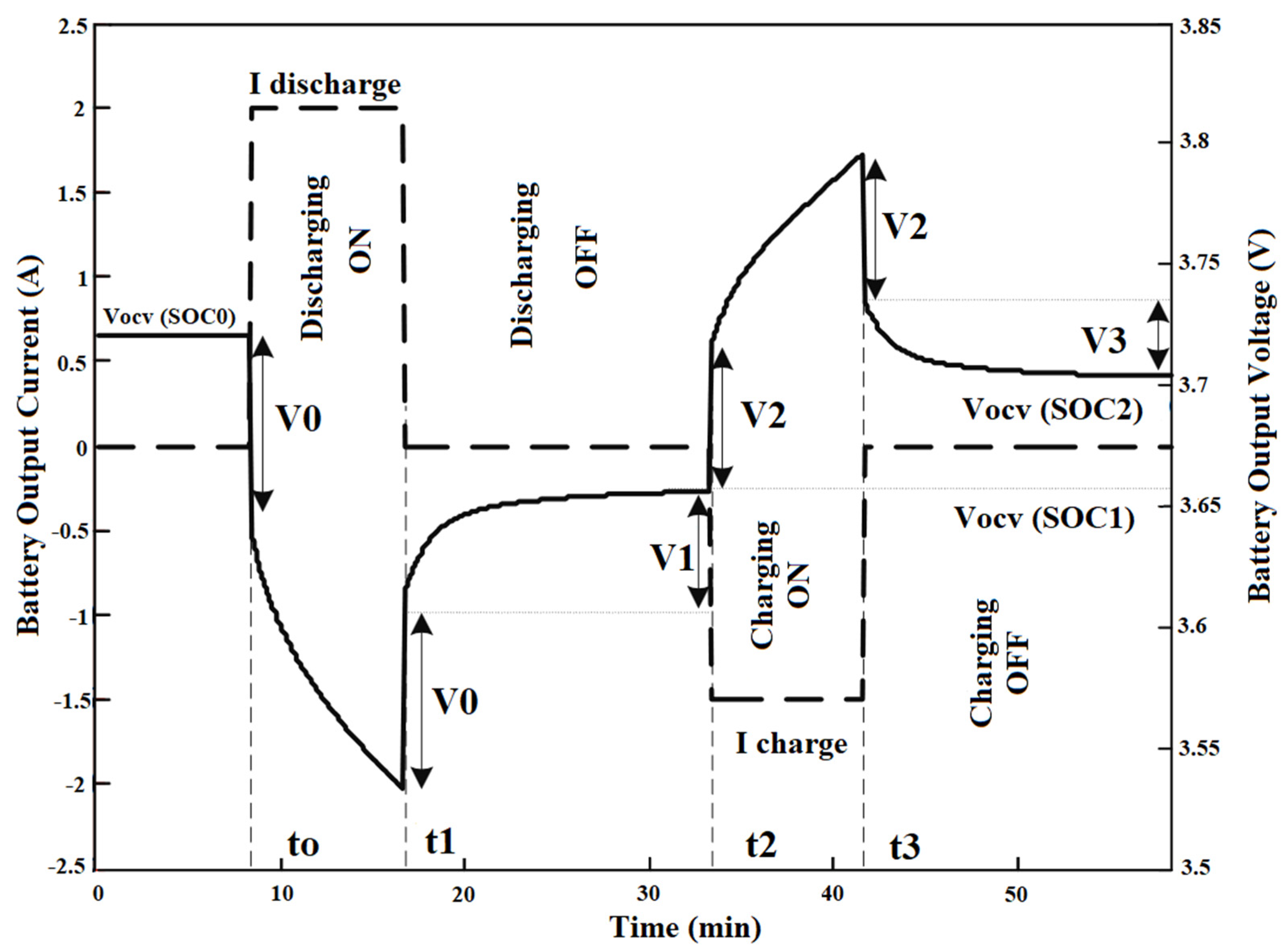
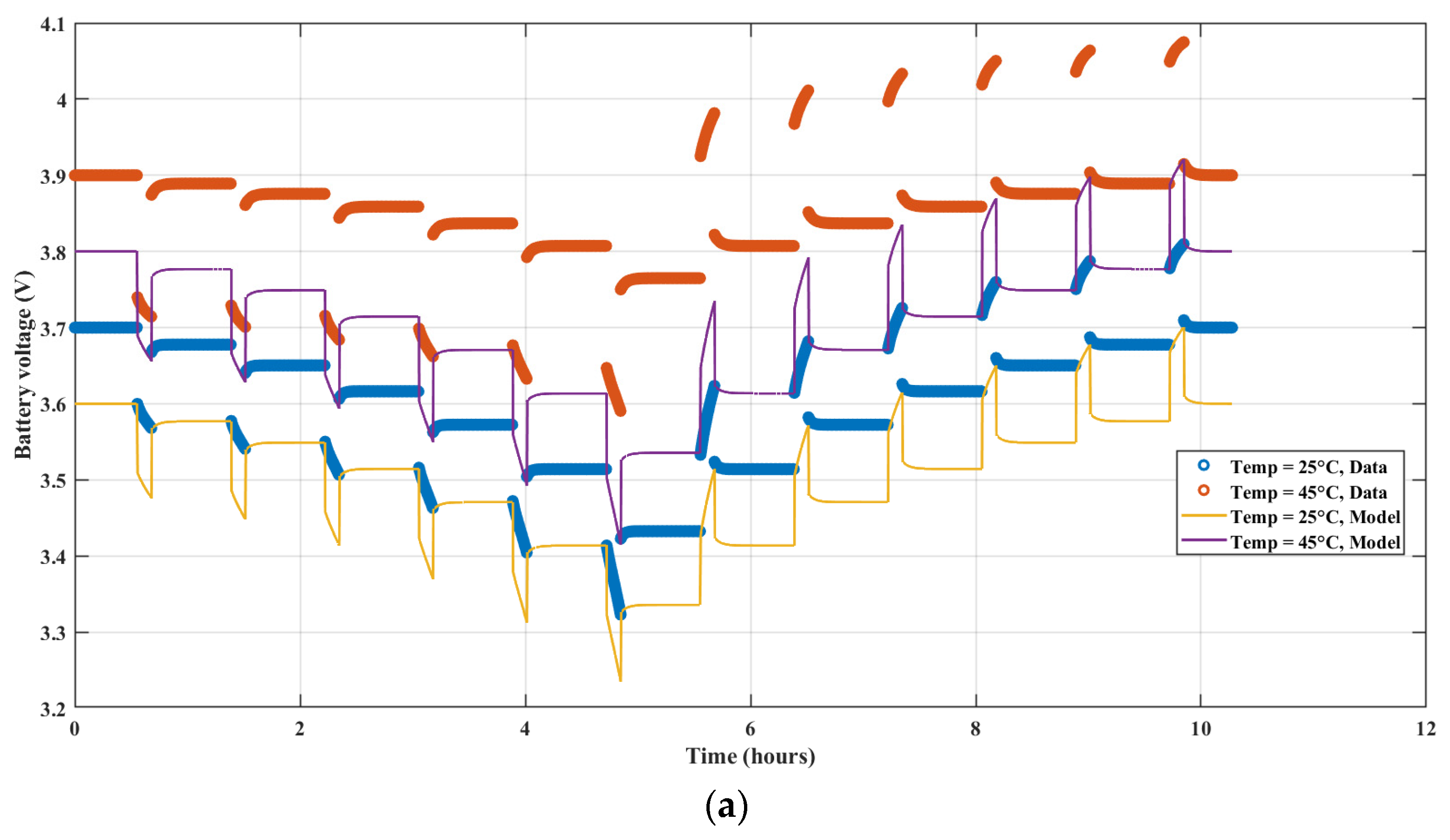
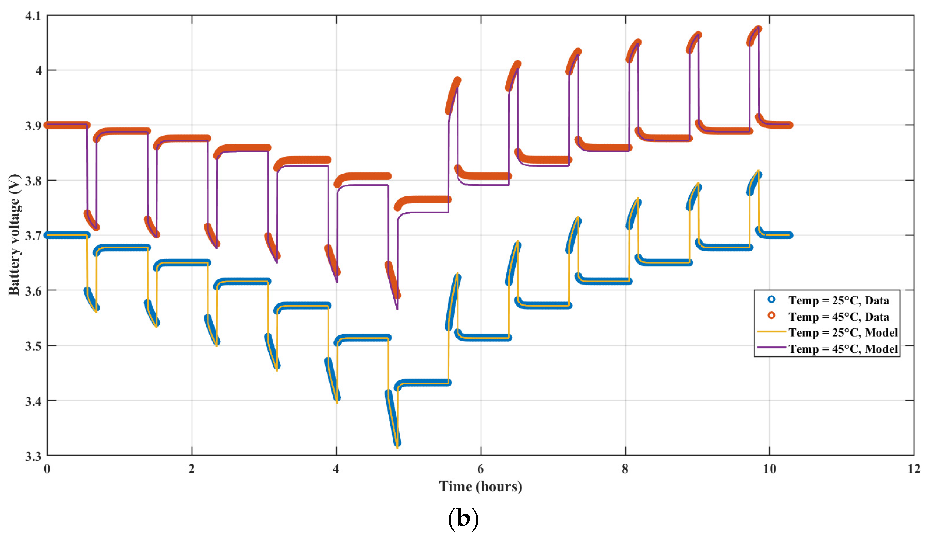
Battery model parameter estimation has emerged as a significant obstacle to correctly modeling these components’ effects on the entire system’s operation. Finding the most appropriate prediction to simulate the battery is still an active area of research. Since the battery is presented in a nonlinear problem, the state of charge is a factor in this problem, which is a critical requirement for achieving the proper supervision and control of battery charging and discharging. The battery parameters are determined for the different modeling forms using experimental approaches. In addition, accurate prediction of the battery’s properties and SOC is essential for several reasons, including extending battery life, controlling the battery’s state of charge, improving battery performance, improving energy management, and monitoring and reporting on battery safety.

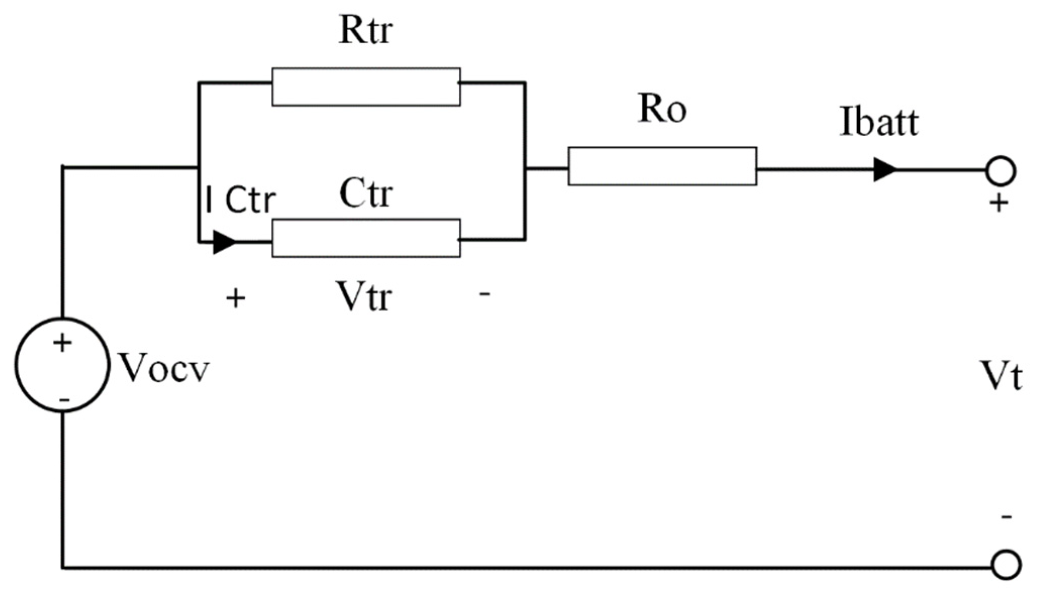
Lithium-ion battery modeling is carried out by estimating the parameters of the battery’s equivalent circuit: the battery’s internal resistance, the polarization branches consisting of resistances and capacitances, and the battery’s open-circuit voltage at different states of charge. The parameters of lithium-ion batteries need to be adequately estimated to extend the battery’s lifespan and to ensure the safe and dependable operation of lithium-ion batteries [17]. To guarantee the safety, longevity, and optimum performance of the battery, the Li-ion battery needs precise parameter estimation of the battery since accurate parameter estimation for the battery results in minimizing the error between the real data and the experimental data, which results in accurate modeling for the battery which helps in the stage of studying the dynamic analysis of the battery [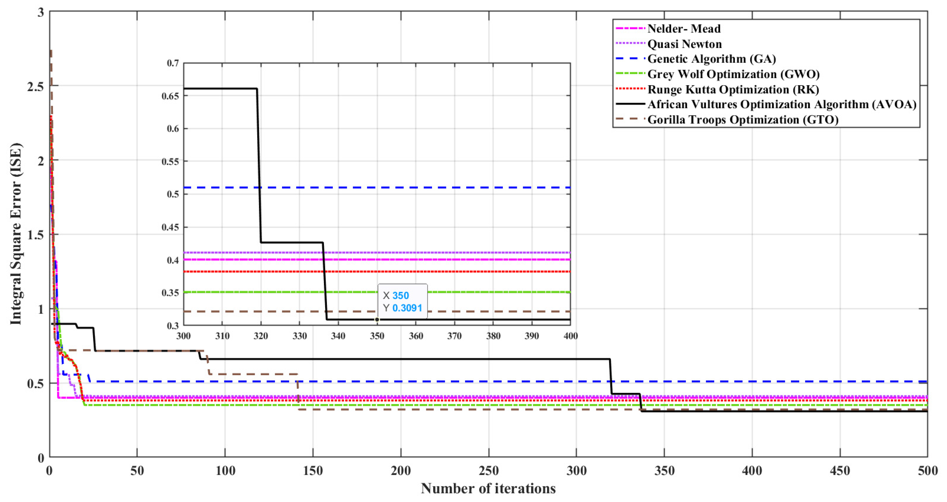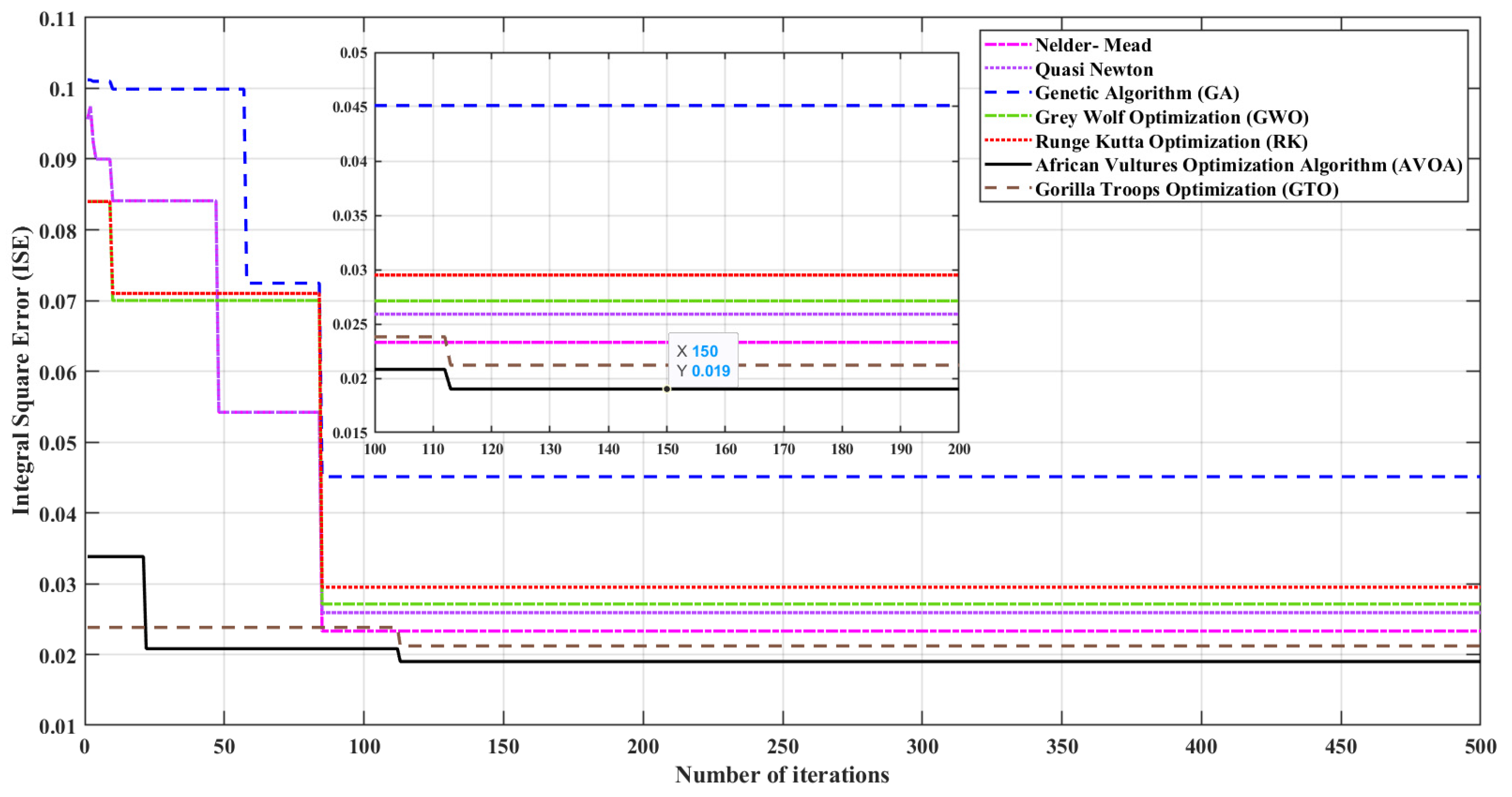18]. The main goal is to acquire an accurate parameter model for lithium-ion batteries by using a precise state space model produced from an equivalent electric circuit where the parameter identification process is nonlinear because of the high complexity of the electrochemical process inside the lithium-ion battery. The African vultures optimization algorithm (AVOA) was used to solve this problem by simulating African vultures’ foraging and navigating habits. The AVOA was used to implement this strategy and improve the quality of the solutions. Four scenarios varied between considering the loading and fading effect of a lithium-ion battery, and its dynamics were considered. 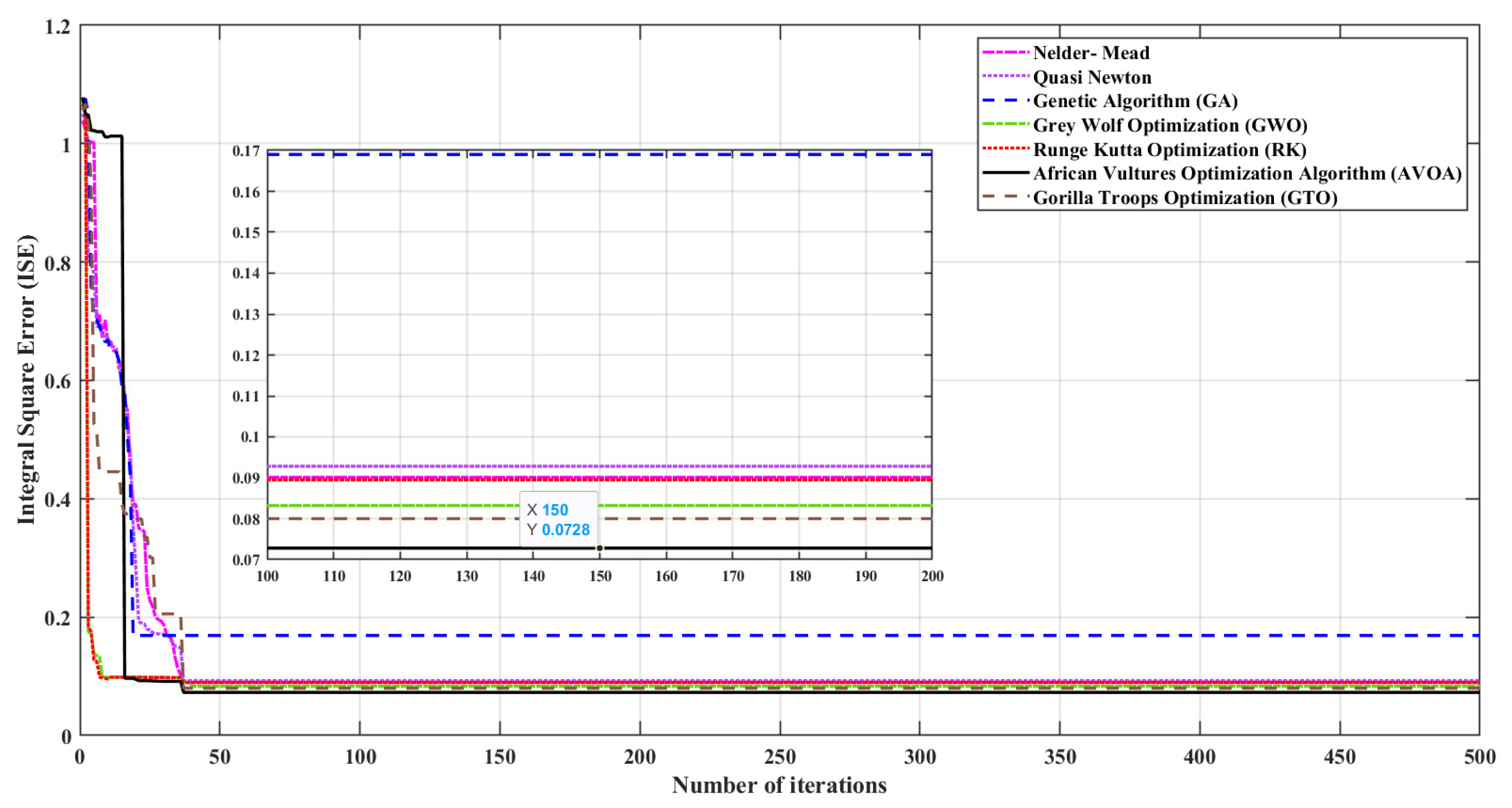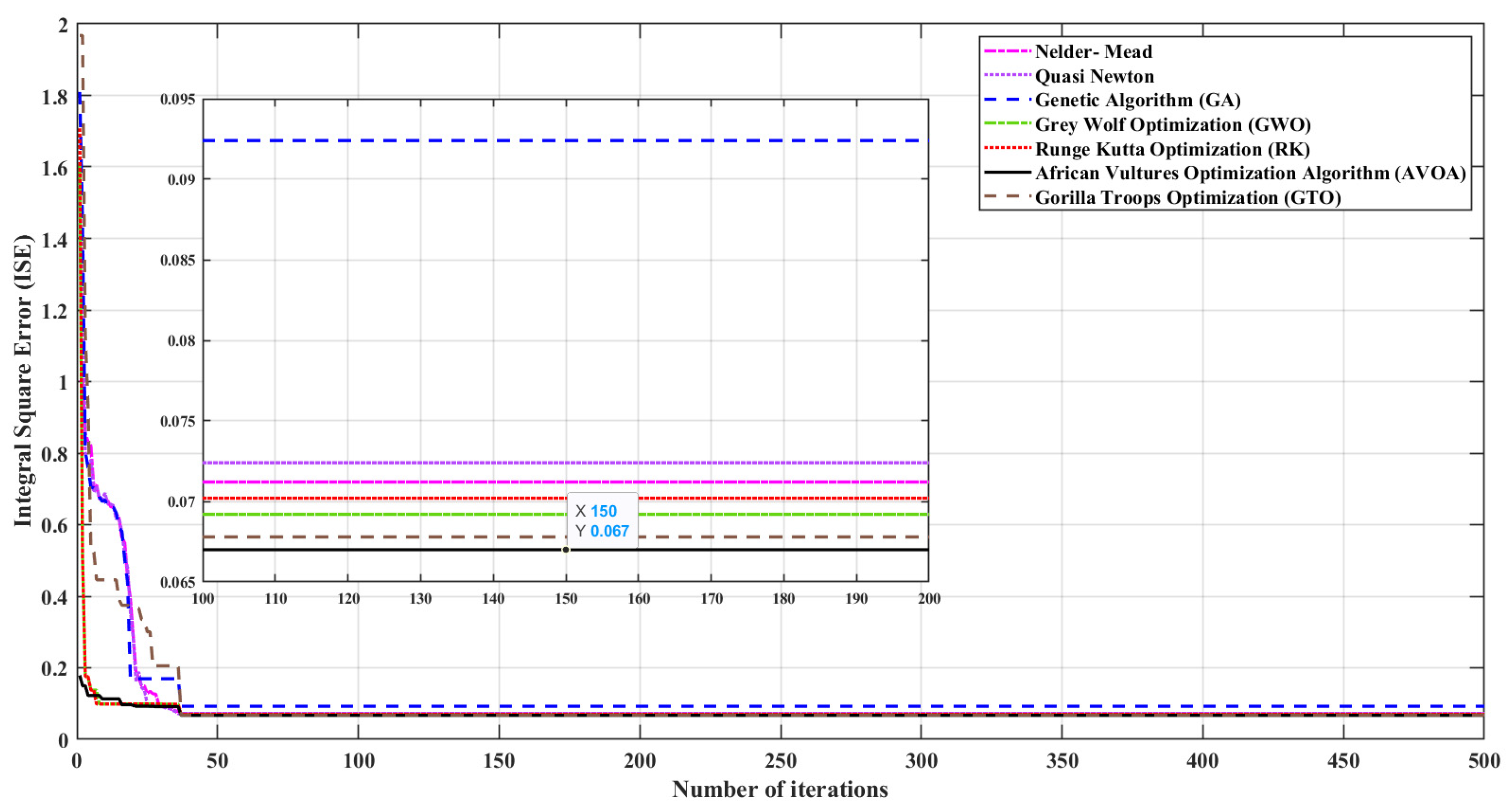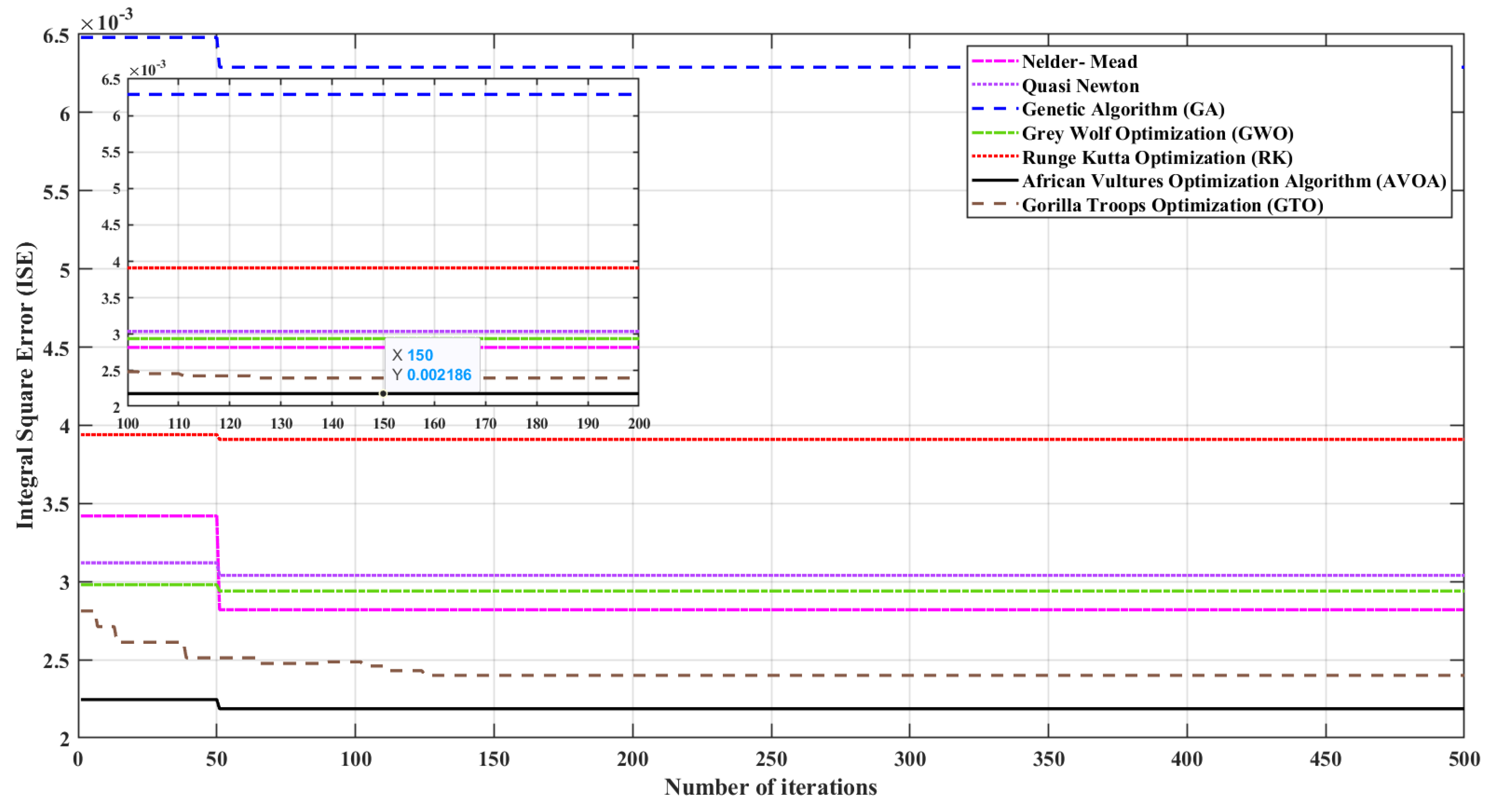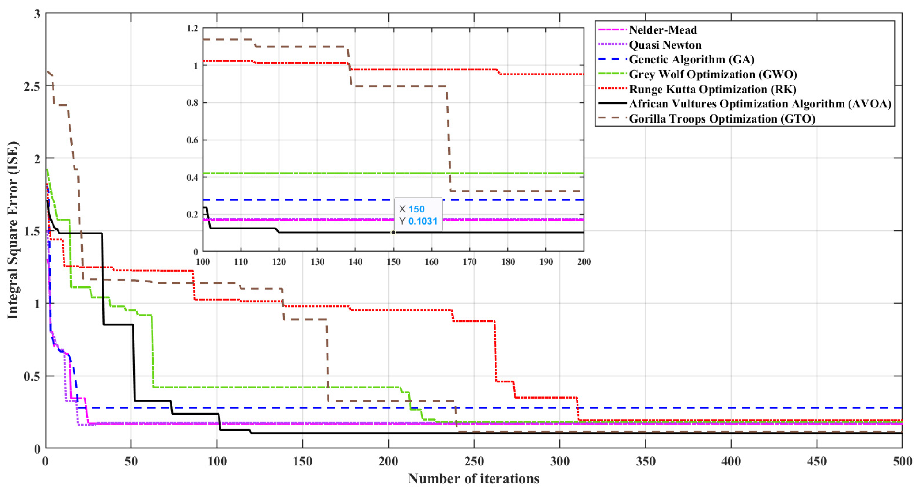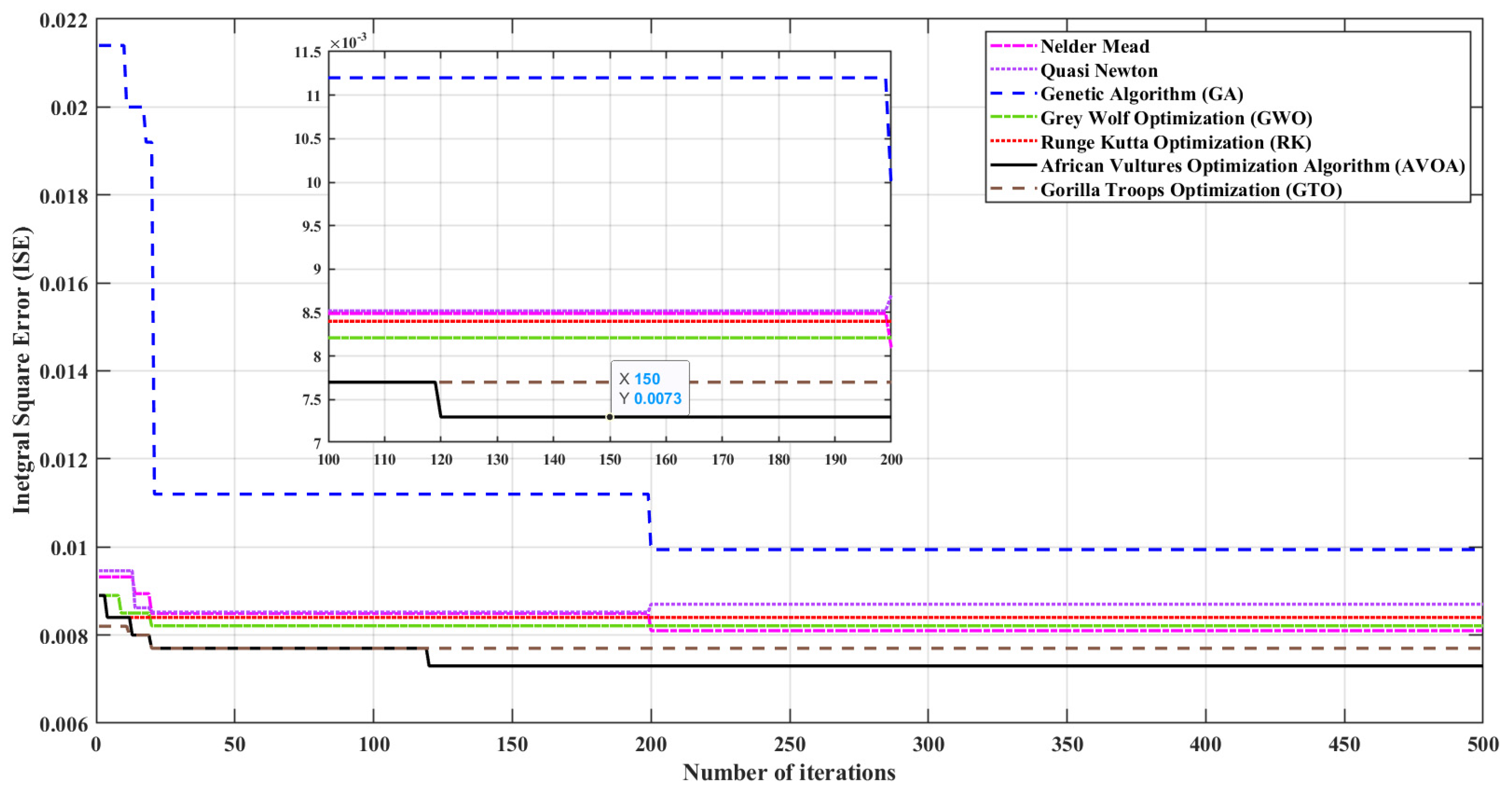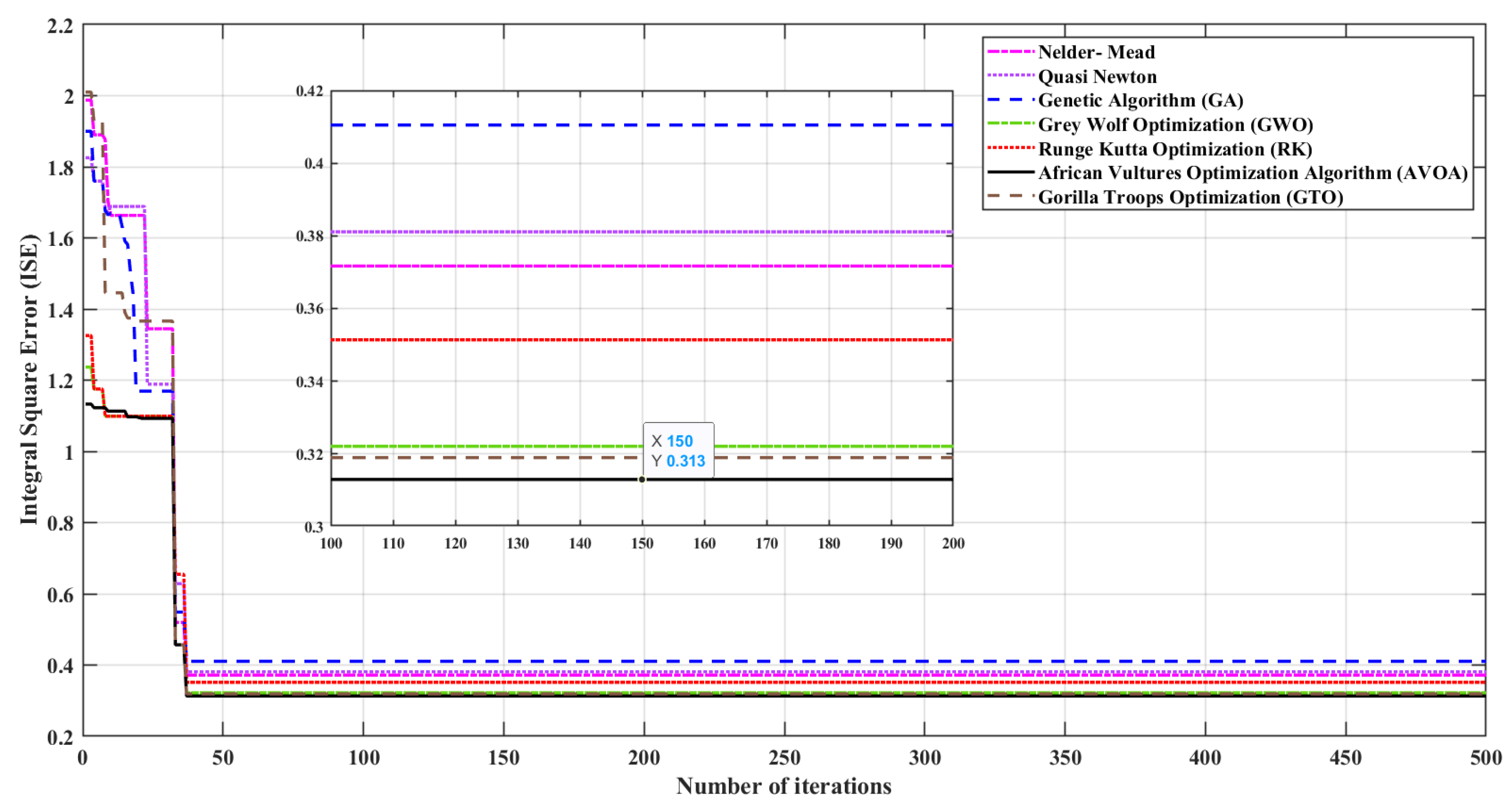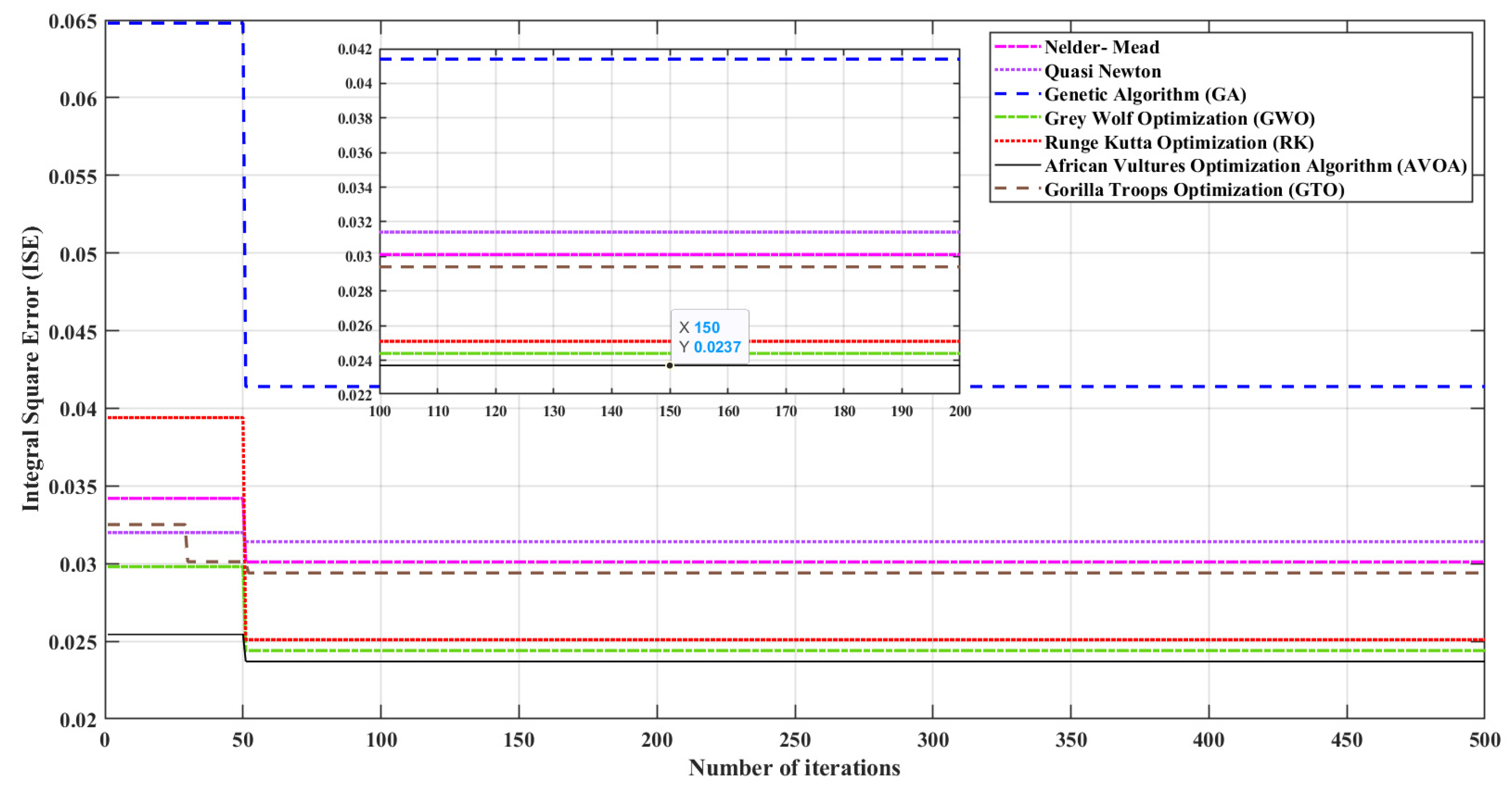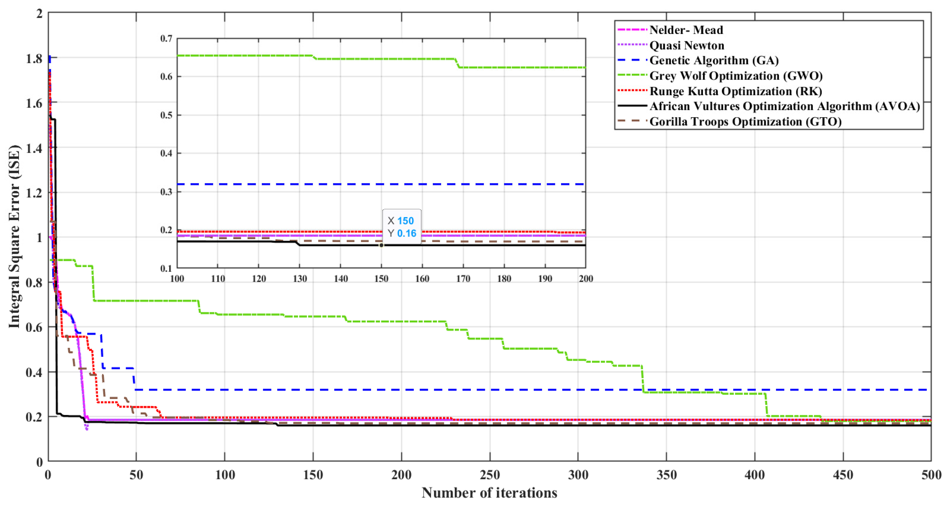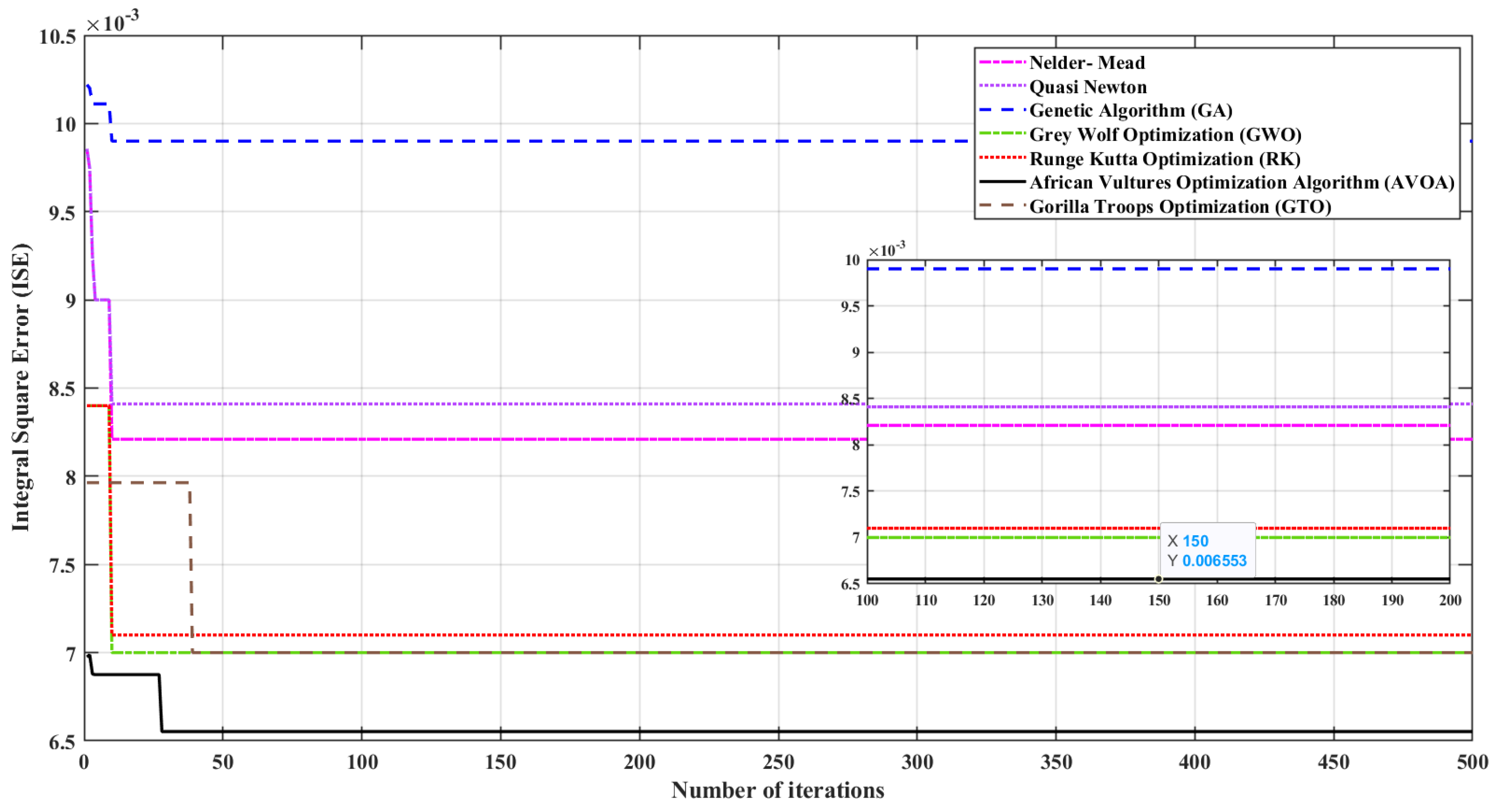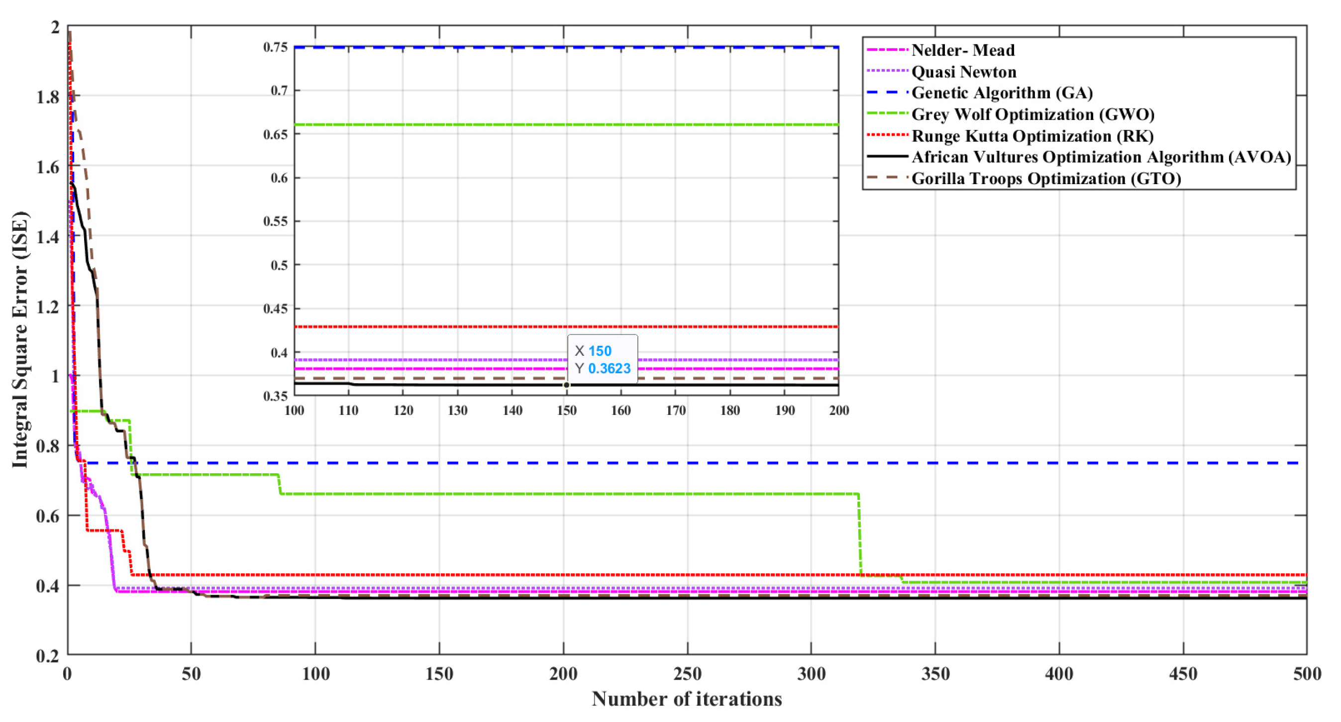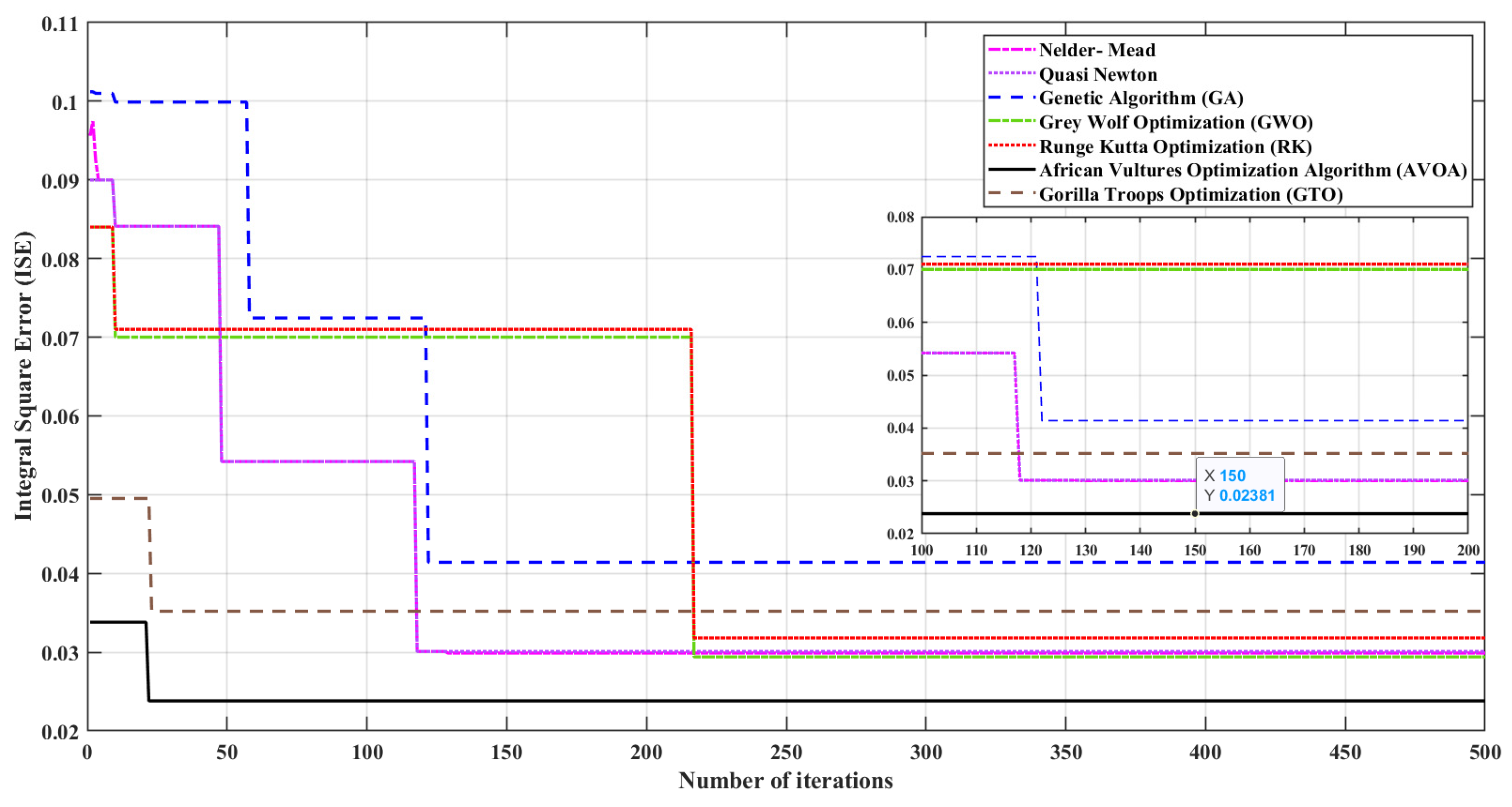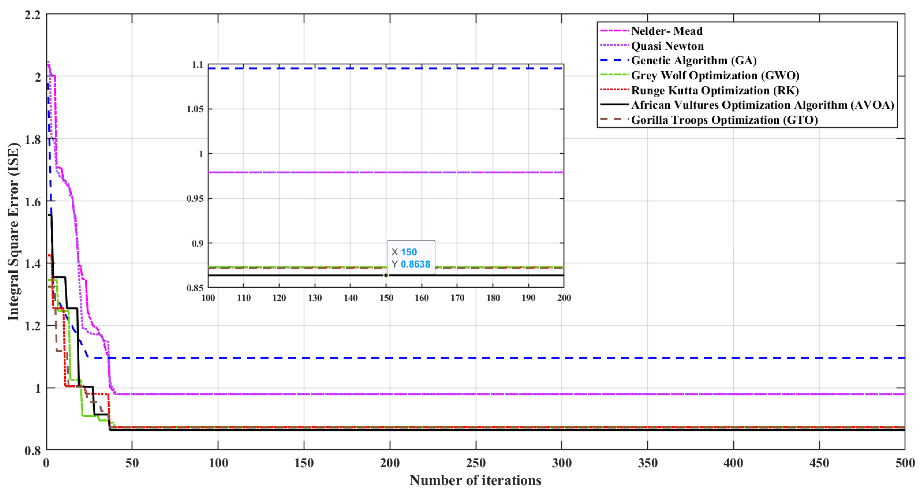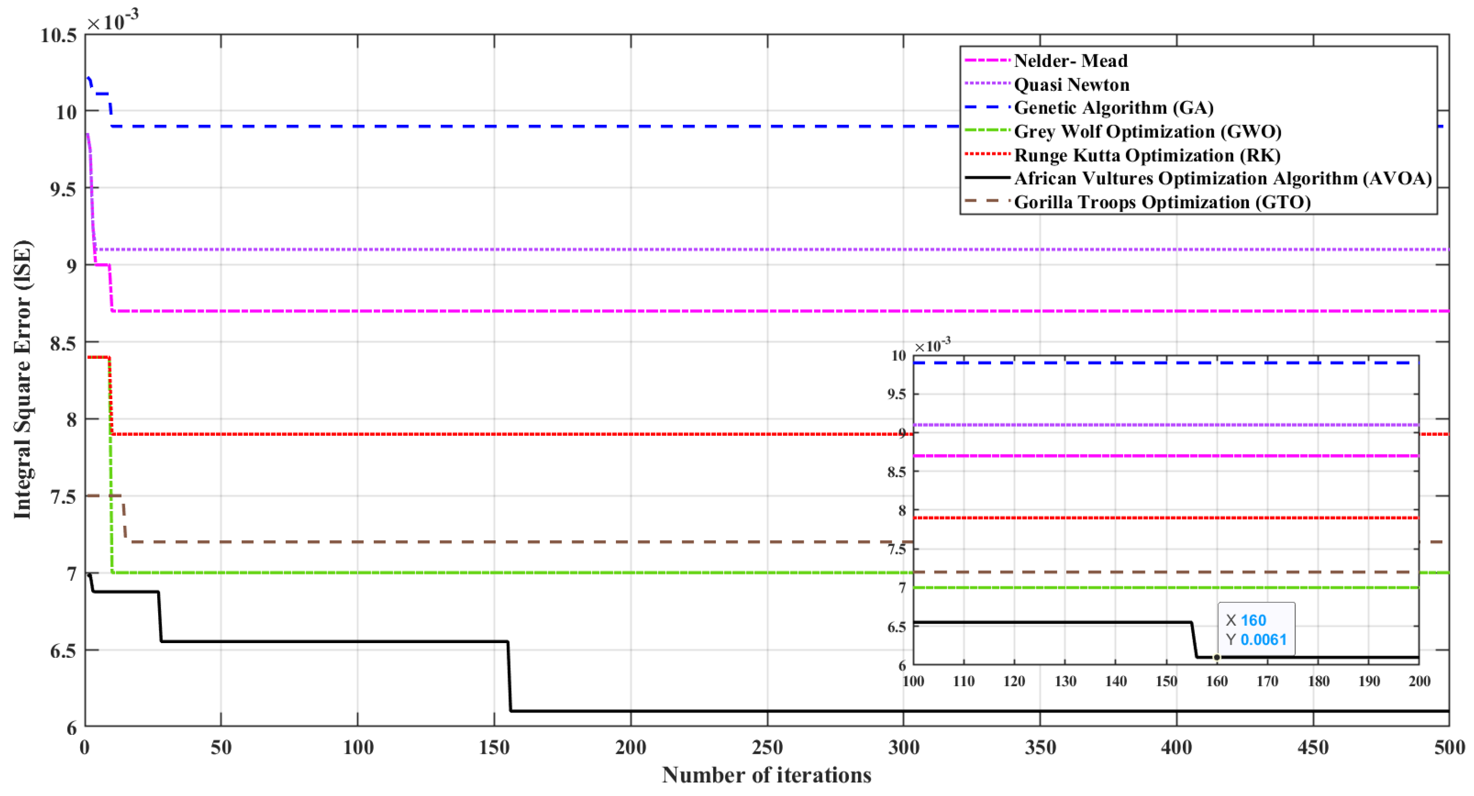The ISE is the fitness function. Numerical simulations were executed on Li-ion batteries to demonstrate the effectiveness of the suggested parameter identification technique. The proposed AVOA was compared with different algorithms such as the Nelder–Mead simplex algorithm, the quasi-Newton algorithm, the Runge Kutta optimizer, the genetic algorithm, the grey wolf optimizer, and the gorilla troops optimizer.

1.2. Literature Review

Accurate parameter estimation for SOC estimation is a challenging problem due to lithium-ion batteries’ very nonlinear and complicated electrochemical nature [19]. Several techniques have been used for the parameter and SOC estimates, including the data-driven approach, non-model-based techniques, and model-based techniques [20]. Despite the computational efficiency of these approaches, they have the drawbacks of gathering sensor errors and taking a long time to process precise parameter and SOC estimates. Technologies based on artificial intelligence that are inspired by biology, including genetic algorithms [21], bacterial foraging algorithms [22], particle swarm optimization [23], and firefly algorithms [24], are mainly used.

Lai et al. [25] performed a comparative analysis to identify the most effective global optimization techniques for identifying the parameters of several lithium-ion battery types. They demonstrated that exact algorithms are the best option for first-order resistance–capacitance (RC) models. At the same time, the particle swarm optimization method is the best identification approach for second-order RC models. The firefly algorithm has the maximum accuracy for third- and fourth-order RC models. The computational complexity of genetic and bacterial foraging methods is high, whereas parameter tuning for particle swarm requires a significant effort. The approaches based on computer intelligence give advantages, including noise cancellation, high accuracy, and quick convergence rate, by utilizing adaptive strategies for SOC estimation.

Single- and double-RC-branch circuit models are widely used in model-based methods to simulate the lithium-ion battery [26]. The battery model’s parameters are determined either offline or online. When determined offline [27,28], a hybrid pulse power characteristic approach is utilized to calculate the battery model parameters, which are then used to estimate the parameters. Using the fixed experiments as a reference, these parameters are calculated. However, in real time, these factors alter due to aging, temperature, dynamic working circumstances, etc., which directly impacts SOC estimates [29,30]. Consequently, for proper SOC estimation, these parameters should be evaluated online. Data-driven strategies have been presented to address the shortcomings of the two prior approaches [31]. Through artificial intelligence techniques [32], neural networks [33], machine learning [34], support vector machines [35], and fuzzy logic [36], this method determines the most exact correlation between the battery’s state of charge and its measurable data, such as current, voltage, and temperature [37]. Because of their excellent learning capacity, these approaches could comprehend the battery’s internal dynamics via several charging and discharging cycles. The emergence of the latest deep-learning algorithms has led to a gradual improvement in learning accuracy thanks to the accumulation of previously learned data that enable precise SOC estimates [38]. These methods do, however, have significant drawbacks. They first require a large amount of data to train and evaluate the model [39]. The complicated topology of such a neural network makes it challenging to adjust the deep-learning parameters [40]. These methods also use up a large amount of memory space and take longer to calculate. There are more parameters and SOC estimating techniques in the literature. The internal electrochemical reactions of the battery have frequently used electrochemical impedance spectroscopy [41]. The internal resistance technique uses rapid voltage and current readings to measure the battery’s capacity. It is used to evaluate the battery’s state of charge [42]. A detailed battery model is required for model-based SOC estimation. This model can improve the simulation efficiency in addition to the SOC estimation [43]. The literature might separate equivalent circuit and electrochemical models [44]. Due to its simplicity, the first category is frequently used for state-of-charge estimation and electric vehicle simulation.

Nonetheless, the number of RC branches employed determines how accurate this model is; however, the model becomes increasingly difficult for users when the number of RC branches is increased to attain accuracy, affecting parameter identification and SOC estimation [45]. Parameter identification interests many academics due to its significance for various model-based SOC estimations [46,47], such as the neural network, genetic algorithm [48], optimization algorithm, and least square identification [49]. Optimization algorithms are better suited for parameter identification than neural network algorithms due to their simplicity and ease of setting. The study that goes along with it illustrates the significant efforts made to accurately and methodically assess the features of energy storage devices powered by Li-ion batteries. Although these methods have produced acceptable results, they lack precision and consistency. This paper suggests the involvement of loading and fading in identifying lithium-ion battery parameters by minimizing the error between the measured and experimental voltage using the integral square error method $\left(ISE\right)$. Identifying the battery model parameters ensures the best battery performance and a long lifetime. The design parameters are identified using old and new optimization techniques under different loading, fading, and temperature conditions. The design parameters identified are the open-circuit voltages under different SOC, internal resistance, and polarization branches, which were identified by establishing the African vultures optimization algorithm (AVOA) [50,51], a metaheuristic algorithm with natural inspiration. The African vultures optimizer simulates the foraging and navigational habits of African vultures. According to experimental findings, the AVOA performs better than any other algorithm on 30 of 36 benchmark functions and most engineering case studies. The AVOA was created to validate the integrated square error (ISE) of the objective function of the dynamic lithium-ion battery model. These specific skills provide the AVOA with an exceptional ability to find the best solutions. Despite its advantages, it has not yet been applied to engineering optimization problems.

1.3. Main Contributions

The following are this paper’s main contributions:

• This study considers different loading, fading, and temperature conditions.
• This study uses the AVOA to uncover the Li-ion battery model’s unknown parameters.
• A robust nonlinear link shows the relationship between the open-circuit voltage and the SOC by evaluating the first-order resistive–capacitive version of the Li-ion battery dynamic model.
• Investigations using simulations and Li-ion battery experiments are coupled.
• The AVOA findings are compared with several algorithms, such as the Nelder–Mead simplex algorithm [52], the quasi-Newton method [53], and the Runge Kutta optimizer (RK) [54], and metaheuristic algorithms such as the genetic algorithm (GA) [55], the grey wolf optimizer (GWO) [56], and the gorilla troops optimizer (GTO) [57].
• This study covers the gap of not including loading, battery aging, and temperature conditions in previous research.

1.4. Paper Organization

The remainder of this paper is presented as follows: Section 2 describes a dynamic representation of the Li-ion battery issue using optimization. Section 3 introduces the AVOA methodology. Section 4 reveals the results of the AVOA’s simulation when used to address the problem with Li-ion batteries. Section 5 explains the study’s key conclusions.

2. Problem Identification

Several factors are considered for modeling the battery parameters’ identification and SOC estimate, and the literature’s earlier research did not consider nonlinear modeling’s effects. In addition, a complex state space model is the foundation for many models reported in the literature. The linear model does not require much calculation time for parameter identification. Nevertheless, because the Li-ion battery model is a nonlinear system, nonlinear models can provide excellent parameter estimate accuracy but take more time to compute. Compared with traditional nonlinear models, the suggested technique has resulted in the development of a simplified nonlinear model with high identification accuracy and less computing time. Then, the solution approach has a significant impact on parameter estimates. A simplified model with sufficient accuracy for parameter estimates must be proposed to solve this issue. The previously identified research gaps in the literature are the subject of the current study. In this regard, a nonlinear representation of the relationship between open-circuit voltage and the state of charge is considered due to the instability of the internal chemical processes within the battery.

2.1. Modeling of Lithium-Ion Batteries

To comprehend the dynamic behavior of lithium-ion batteries, a thorough battery model must be chosen [58]. Various lithium-ion battery models were displayed and compared in terms of their complexity and accuracy; the more advantageous choice was a network-based battery model with single and double RC branches and lumped parameters. The single-order RC model, the one-time constant model of the lithium-ion battery, is the most frequently used and was chosen for this paper, as shown in Figure 1 [59].

This model mainly consists of three parts, which are as follows: a battery voltage source, which is called battery open-circuit voltage ($V_{ocv}$), internal ohmic resistance ($R_o$), and a resistance and capacitance branch, which describes the battery’s transient behavior while being charged and discharged ($R_{tr},C_{tr}$) and is called the charge dynamics of the battery. ($V_{tr}$) and ($I_{Ctr}$) are the voltage across and the current of the transient capacitance ($C_{tr}$) and ${(I}_{batt})$ is the battery’s terminal current.

The one-time constant model’s electrical behavior may be described by Equations (1) and (2):

$$V_{tr}=\frac{-1}{R_{tr}\times C_{tr}}{V}_{tr}+\frac{1}{C_{tr}}{I}_{batt}$$

(1)

$$V_t=V_{ocv}-V_{tr}-R_o\times I_{batt}$$

(2)

The discrete-time description is shown in Equations (3) and (4) as follows:

$$V_{tr},k+1=V_{tr},k{e}^{\frac{-{\tau }_s}{{\tau }_{tr}}}+R_{tr}\left(1-e^{\frac{-{\tau }_s}{{\tau }_{tr}}}\right)I_{batt},k$$

(3)

$$V_t,k=V_{ocv}\left(SOC,k\right)-V_{tr},k-R_o\times I_{batt},k$$

(4)

where ${\tau }_s$ is the sampling time and ${\tau }_{tr}$ is the transient branch time constant.

Equation (5) describes how the battery’s open-circuit voltage depends on its charge level ($SOC$).

$$V_{ocv}=V_{nom}\left(\frac{SOC}{1-\beta (1-SOC)}\right)$$

(5)

where ${(V}_{ocv})$ is the open-circuit voltage of the battery, which is equal to ${(V}_{nom})$, which is the open-circuit voltage when the battery is fully charged ($SOC=1$), which is the voltage which is called nominal voltage, and it is equal to ${(V}_{dis})$, which is the open-circuit voltage when the battery begins to discharge $(SOC<1)$ at constant battery discharge capacity ($Q_{dis}$), and (β) is the battery fade coefficient.

To calculate the state of charge of the battery, Equation (6) is used as follows:

$$SOC=SO{C}_{°}-\frac{1}{Q}{\int }_0^t{I}_{batt}dt$$

(6)

where $\left(Q\right)$ is the battery capacity in ampere-hours. By using Equation (6), $SOC$ is calculated to calculate $V_{ocv}$ in Equation (5) and then calculate the value of terminal voltage $\left(V_t\right)$ in Equation (4).

• Battery Fade Calculation

The term “battery fade” refers to the degradation of battery performance over several charge and discharge cycles, which is modeled as follows:

According to Equation (7), the open-circuit voltage across the basic battery model decreases proportionately to the number of discharge cycles $n$.

$$V_{nom,fade}=V_{nom}\left(1+\frac{{\delta }_{vnom}\times n}{100\times N}\right)$$

(7)

where ${\delta }_{vnom}$ is the percent change in open-circuit voltage after $N$ discharge cycles.

According to Equation (8), the nominal charge, from which the state of charge is determined, decreases with the square root of the number of discharge cycles:

$$Q_{fade}=Q\left(1+\frac{{\delta }_Q}{100}\sqrt{\frac{n}{N}}\right)$$

(8)

where ${\delta }_Q$ is the percent change in battery capacity after $N$ discharge cycles.

All resistances in the battery model also fade with the square root of the number of discharge cycles, as presented in Equation (9):

$$R_{i,fade}=R_i\left(1+\frac{{\delta }_{Ri}}{100}\sqrt{\frac{n}{N}}\right)$$

(9)

where $R_i$ is the $i\mathrm{t}\mathrm{h}$ resistance, which is $R_o$ (internal resistance of the battery) and $R_{tr}$ (transient resistance of the battery), and ${\delta }_{Ri}$ is the percent change in battery internal/transient resistance after $N$ discharge cycles.

This part shows how to estimate the model parameters using battery readings. The battery’s experimental parameters were identified using the first method at a temperature of 25 °C; the temperature, aging, and loading are considered as this work progresses. As the battery is being charged and discharged, the output voltage and current characteristic curves are shown in Figure 2, and different intervals of the curves are explained.

• Interval $i_0(t<t_o$): In this interval, for a long enough period, the battery output current can be taken to be zero, even though the output voltage might equal the open-circuit voltage value $\left(V_{ocv}\left(SO{C}_0\right)\right)$, and the ($SOC)$ value remains constant when the output current is zero.
• Interval $i_1(t_o\le t\le t_1)$: In this interval, constant current discharges the battery $(I_{discharge}>0)$; due to the internal resistance ${(R}_o)$, the battery output voltage first drops significantly, then it keeps decreasing exponentially under the control of the $OCV$ (during the $SOC$ decrease).
• Interval $i_2(t_1\le t\le t_2)$: In this interval, the value of the battery output current is zero $(I_{batt}=0)$, hence $\left(R_o\right)$ initially causes a sharp increase in the battery output voltage and, after that, an exponential rise until it reaches ${(V}_{ocv}\left(SO{C}_1\right))$ can be observed.
• Interval $i_3(t_2\le t\le t_3)$: In this interval, constant current charges the battery $(I_{charge}<0)$; due to internal resistance ${(R}_o)$, the battery output voltage gradually increases, and then it continues to increase exponentially under the control of the $OCV$ (during the $SOC$ increase).
• Interval $i_4(t\ge t_3)$: In this interval, the value of the battery output current is zero ${(I}_{batt}=0)$, hence ${(R}_o)$ initially causes a sharp decrease in the battery output voltage and, after that, an exponential fall until it reaches ${(V}_{ocv}\left(SO{C}_2\right))$ is observed.

For the internal ohmic resistance of the battery $\left(R_o\right)$, the voltage drops across $\left(R_o\right)$ during the initial moment of charging $\left(V_2\right)$ and discharging $\left(V_0\right)$; this may be used to compute $\left(R_o\right)$ according to Equation (10):

$$R_o=\left\{\begin{array}{c}\frac{V_0}{I_{discharge}}, For discharging\hfill \\ \frac{-V_2}{I_{charge}}, For charging\hfill \end{array}\right.$$

(10)

Readings of the battery’s output voltage at periodic intervals $i_2$ and $i_4$ are used, as $OCV$ remains constant during these times, and the battery’s dynamic properties are the only factors that affect the output voltage. The output voltage $V_t$ during $i_2$ and $i_4$ can be computed according to the model by setting $I_{batt}$ to zero in Equations (3) and (4); the differential equation is then resolved as indicated in Equation (11):

$$\left\{\begin{array}{c}i2:V_t(t)=V_{ocv}(SO{C}_1)-V_{tr}(t_1)e^{\frac{-t}{{\tau }_{tr}}}\\ i4:V_t(t)=V_{ocv}(SO{C}_2)-V_{tr}(t_3)e^{\frac{-t}{{\tau }_{tr}}}\end{array}\right.$$

(11)

where ${\tau }_{tr}=R_{tr}\ast C_{tr}$.

2.2. Objectives of Lithium-Ion Battery Parametrization Problem

• Constraints

Applying the battery’s dynamic model covered in the previous part, the battery parameters are recognized, and the state of charge is approximated. An objective function must be developed to fit the predicted output voltages with the corresponding observed voltage in the experimental testing to optimize the Li-ion battery model’s features. The recommended objective function is founded on reducing the integrated square error $\left(ISE\right)$ between experimental data and the outcomes of model-based simulations. The proposed optimization issue is represented as the following in Equation (12).

$$\begin{gathered} Mi{n}_{u}Fi\left(u\right),i=\mathrm{1,2},\dots n\_obf \\ Umin\le U\le Umax \end{gathered}$$

(12)

$F_i\left(u\right)$ is the objective function, and $i$ and $u$ represent the parameters that need to be estimated in the battery. The control variable vector’s parameter boundaries, which reflect the permitted research domain, are $Umin$ and $Umax$, and $n_{obf}$ is the total number of objective functions. The model’s input parameters are determined using the data from the battery experiment.

The primary objective of the challenge at hand is to minimize the integral square error between the experimental and estimated battery voltage $F_i\left(u\right)$ using Equation (13).

$$F_i\left(u\right)=\sum {\left(V_{estimated}–V_{experimental}\right)}^2$$

(13)

where $V_{estimated}$ is the expected battery model voltage in volts and $V_{experimental}$ is the recorded experimental battery voltage.

The model input parameters are represented as follows: $V_{nom}$: battery open-circuit voltage at $SOC=1$, which is called nominal voltage; $V_{dis}$: battery open-circuit voltage when the battery begins to discharge $(SOC<1)$ at constant battery discharge capacity ($Q_{dis}$); $R_o$: internal ohmic resistance; $R_{tr}$: transient resistance of the battery; ${\tau }_{tr}$: transient time constant; $Q$: battery capacity in ampere-hours.

The objective function is solved under the following constraints:

$Qmin\le Q\le Qmax$
$R_{o}min\le R_o\le R_{o}max$	$\mathrm{at} T_1=25 °\mathrm{C} \mathrm{and} T_2=45 °\mathrm{C}$
$R_{tr}min\le R_{tr}\le R_{tr}max$	$\mathrm{at} T_1=25 °\mathrm{C} \mathrm{and} T_2=45 °\mathrm{C}$
${\tau }_{tr}min\le {\tau }_{tr}\le {\tau }_{tr}max$	$\mathrm{at} T_1=25 °\mathrm{C} \mathrm{and} T_2=45 °\mathrm{C}$

where $min$ and $max$ are the minimum and maximum operators of the parameters, respectively.

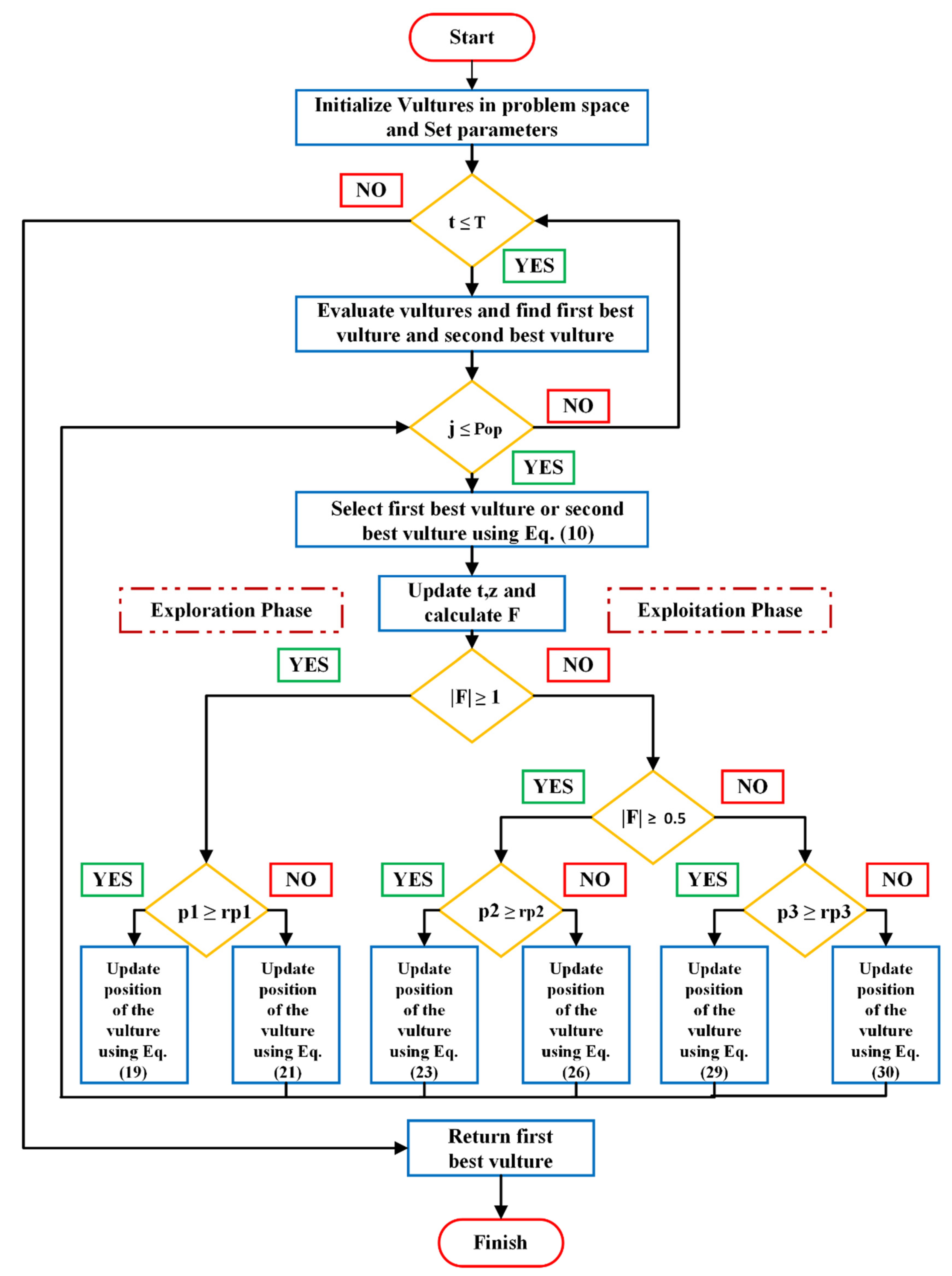
3. African Vultures Optimizer Methodology

Abdollahzadeh et al. introduced the AVOA metaheuristic algorithm in 2021, and it has since been used in numerous real-world engineering projects [60]. By replicating and modeling the feeding activity and dwelling habits of African vultures, AVOA was first proposed. African vultures’ daily routines and foraging behavior are replicated in AVOA.

The population of African vultures consists of $N$ vultures, and the algorithm user determines the size of $N$ based on the current circumstances. Each vulture’s position space has $D$ dimensions, with the size of $D$ varying according to the dimension of the problem being handled. It is crucial to decide on a maximum number of iterations T in advance proportional to the complexity of the issue that needs to be solved and represents the most activities the vulture can perform. As a result, each vulture’s position $i\left(1\le i\le N\right)$ at various iterations $t\left(1\le t\le T\right)$ can be written as Equation (14):

$$x_i^t=\left[x_{i1}^t\dots x_{id}^t\dots x_{iD}^t\right]$$

(14)

where $x_i^t$ is the vulture’s position, t is the number of iterations, and D is the dimension of each vulture’s position. Vultures in the population can be split into three types based on their lifestyles in Africa. The first flock is tasked with identifying the best viable solution among all vultures if the fitness value of the feasible solution is being utilized to gauge the quality position of the vultures. According to the second flock, the practical solution is the second-best vulture overall. The remaining vultures are grouped into a third flock in addition to the first two flocks mentioned, and they all forage together throughout the population. As a result, different vulture species have different functions within the population. If it is thought that the population’s fitness value can depict the benefits and drawbacks of vultures; the worst vultures are the ones that are the most vulnerable and voracious. The best vulture at this time, though, is the one that is strongest and most prevalent. All vultures in AVOA attempt to approach the superior vulture and avoid the poor vultures. To mimic various vulture actions during the foraging phase, AVOA can be separated into five stages according to the four rules of behavior.

Stage 1: Population Grouping: The second rule states that the vultures must be categorized according to their quality after startup or before beginning the subsequent action. The vulture representing the ideal solution is put in the first flock, while the vulture representing the runner-up is put in the second flock. The third flock has the remaining vultures. Due to the directing effects of the best and second-best vultures, Equation (15) aims to choose the vulture the current iteration should advance towards and move towards the best solutions for the first and second groups. In each fitness iteration, the entire population is recalculated.

$$R_i^t=\left\{\begin{array}{c}BestVultur{e}_1^t,p_i^t=L_1\\ BestVultur{e}_2^t,p_i^t=L_2\end{array}\right.$$

(15)

where $BestVultur{e}_1^t=\left[b_{11}^t\dots b_{1d}^t\dots .b_{1D}^t\right]$ means the best vulture, and $BestVultur{e}_2^t=\left[b_{21}^t\dots b_{2d}^t\dots .b_{2D}^t\right]$ is the second-best vulture. In Equation (15), the likelihood of picking the chosen vultures to steer the other vultures towards one of the best options in each group is computed, in which L₁ and L₂ are variables that must be measured before the search procedure. The probability of choosing the best solution is gained using the roulette wheel to choose each of the best solutions for each group ($p_i^t$). $p_i^t$ is obtained using a random strategy, and its calculation formula is stated in Equation (16). $L_1$ and $L_2$ are two random values in the range [0, 1], and their sum is 1.

$$p_i^t=\frac{f_i^t}{\sum _{i=1}^m{f}_i^t}$$

(16)

where m is the overall number of the first-flock and second-flock vultures, and the $f_i^t$ is the fitness rating of the first-flock and second-flock vultures. The first flock of vultures is symbolized by $\alpha$, the second flock by $\beta$, and the third flock by $\gamma$. The target vulture is then located using pertinent parameters.

Stage 2: The Vultures’ Hunger: The vulture can go further in search of food if it is not overly hungry. On the other hand, if the vulture is currently very hungry, it lacks the physical stamina to facilitate its regional travel. Therefore, vultures that are starving become highly hostile. Thus, they remain close to the vultures carrying food rather than going out searching for food on their own. Consequently, vultures’ exploration and exploitation stages can be built based on their behavior. Hunger levels indicate when vultures are moving from the exploration stage to the exploitation stage. Equation (17) can be used to determine the degree of hunger $F_i^t$ of the $\left(t\right)\mathrm{t}\mathrm{h}$ vulture at the $\left(T\right)\mathrm{t}\mathrm{h}$ iteration and it is also used to transfer from the exploration phase to the exploitation phase, which is inspired by the hunger behavior of vultures if they are hungry or satisfied.

$$F_i^t=\left(2\times ran{d}_{i1}t+1\right)\times z^t\times \left(1-\frac{t}{T}\right)+g^t$$

(17)

where $ran{d}_{i1}^t$ is a chance number in the range of [0, 1] and $z^t$ is a chance number in the range of [−1, 1]. There is no assurance that when complex optimization issues are solved, the final population after the exploration stage contains precise estimates for the global optimum. Because of this, it results in an early convergence of the best local site. $g^t$ is used to improve efficiency while addressing complex optimization issues, which raises the likelihood that one will successfully escape from local optimum locations. $g^t$ is determined using Equation (18).

$$g^t=h^t\times \left({\sin }^k\left(\frac{\pi }{2}\times \frac{t}{T}\right)+\cos \left(\frac{\pi }{2}\times \frac{t}{T}\right)-1\right)$$

(18)

where $k$ is a predetermined parameter that determines the likelihood that the vulture will carry out the exploitation stage, and $h^t$ is a random number in the [−2, 2] range. A higher $k$ value suggests that the exploration stage is more likely to be entered after the final optimization step. A lower $k,$ on the other hand, suggests that the exploitation stage is more likely to be reached after the final optimization stage. The formula’s design principle states that as the number of iterations increases, $F_i^t$ gradually declines while the decreasing range continues to grow. Vultures start the period of exploration and look for new food in diverse places when $\left|F_i^t\right|$ is greater than 1. Vultures enter the stage of exploitation to pursue better prey around their present position when |$F_i^t$| is lower than 1.

Stage 3: Exploration Stage: In the wild, vultures have superb vision, allowing them to locate dead animals and food quickly. Hence, when searching for food, vultures take a minute to survey their surroundings before starting a long trip to find the food. To determine the vulture’s behavior at this time, the creator of AVOA creates two exploring behaviors and employs a parameter called $p1$. The range of this parameter, $p1$, which is initialized with the algorithm, is [0, 1]. A random value in the range of [0, 1] that is more than or less than $p1$ is used by AVOA to define the vulture’s exploring strategy. To select any of the strategies in the $ran{d}_{p1}$ exploration phase, a random number between 0 and 1 is generated. If this number is greater than or equal to the $p1$ parameter, the first part of Equation (19) is used, but if $ran{d}_{p1}$ is smaller than the $p1$ parameter, the second part of Equation (19) is used. Therefore, Equation (19) can be used to describe the vulture’s exploratory phase.

$$X_i^{t+1}=\left\{\begin{array}{c}{R}_i^t-D_i^t\times F_i^t,p1\ge ran{d}_{p1}^t\\ R_i^t-F_i^t+ran{d}_{i2}^t\times \left(\left(ub-lb\right)\times ran{d}_{i3}^t+lb\right), p1<ran{d}_{p1}^t\end{array}\right.$$

(19)

$X_i^{t+1}$ represents the location of the $\left(i\right)\mathrm{t}\mathrm{h}$ vulture at the $(t+1)\mathrm{t}\mathrm{h}$ iteration, and the random numbers $ran{d}_{p1}^t$, $ran{d}_{i2}^t$, and $ran{d}_{i3}^t$ are uniformly distributed in the range of [0, 1]. $R_i^t$ is acquired by Equation (15), and $F_t$ is acquired by Equation (7). The problem’s solution’s upper and lower limits are represented by $ub$ and $lb$, respectively, and $D_i^t$ is calculated by Equation (20) to show the separation between the existing vulture and its ideal state.

$$D_i^t=\left|C\times R_i^t–X_i^t\right|$$

(20)

In Equation (20), $R_i^t$ is one of the best vultures, selected by using Equation (2) in the current iteration. Moreover, C represents the vultures moving randomly to protect their food from other vultures, where $C$ is inside the range [0, 2] and is obtained by using the formula $C=2\times rand$, where rand is a random number between 0 and 1 and $X_i^t$ denotes the location of the $\left(i\right)\mathrm{t}\mathrm{h}$ vulture at the $\left(t\right)\mathrm{t}\mathrm{h}$ iteration.

Stage 4: Exploitation Stage (Medium): To avoid the imbalance between exploration and exploitation abilities caused by a too-rapid transition of the algorithm in the medium term, the vulture enters the medium-term exploitation stage when the value of $\left|F_i^t\right|$ is between 0.5 and 1. In the medium-term exploitation stage, $p2$, a parameter with a [0, 1] range, is still employed. This parameter decides whether the vulture engages in circular flight or feeding competition. As a result, before the vulture’s act, a random number $ran{d}_{p2}^t$ in the range [0, 1] is created at the beginning of the medium-term exploitation stage. The vultures compete for food when $ran{d}_{p2}^t$ is larger than or equal to parameter $p2$. In contrast, the rotational flying behavior is used when $ran{d}_{p2}^t$ is less than parameter $p2$.

(1)

Food Competition

The vulture becomes full and active when the value of $\left|F_i^t\right|$ is between 0.5 and 1. As a result, when vultures congregate, weak vultures seek to group up and attack the strong vultures to gain food since they are unwilling to share their meal. The weaker vultures try to tire and obtain food from the healthy vultures by gathering around healthy vultures and causing small conflicts, calculated in Equation (21) to model this step.

$$X_i^{t+1}=D_i^t\times \left(F_i^t+ran{d}_{i4}^t\right)–d_i^t$$

(21)

where $D_i^t$ is calculated by Equation (20), $F_i^t$ is calculated by Equation (7), and $ran{d}_{i4}^t$ is an evenly distributed random number in the range of [0, 1]; $d_i^t$ is calculated by Equation (22).

$$d_i^t=R_i^t-X_i^t$$

(22)

(2)

Rotating Flight

In addition to engaging in food rivalry, stuffed and energized vultures also hover above. AVOA uses a spiral model to simulate this behavior. As a result, Equation (23) can represent the vultures’ location update formula in their circular flight behavior.

$$X_i^{t+1}=R_i^t–\left(S_{i1}^t+S_{i2}^t\right)$$

(23)

The spiral model is used to model rotational flight mathematically. A spiral equation is created between all vultures and one of the two best vultures in this method. The rotational flight is expressed using Equations (24) and (25), in which $S_{i1}^t$ and $S_{i2}^t$ are calculated.

$$S_{i1}^t=R_i^t\times \left(\frac{ran{d}_{i5}^t\times X_i^t}{2\pi }\right)\times \cos \left(X_i^t\right)$$

(24)

$$S_{i2}^t=R_i^t\times \left(\frac{ran{d}_{i6}^t\times X_i^t}{2\pi }\right)\times \sin \left(X_i^t\right)$$

(25)

In Equations (24) and (25), $R_i^t$ represents the position vector of one of the best vultures in the current iteration, which is obtained by using Equation (2); $ran{d}_{i5}^t$ and $ran{d}_{i6}^t$ are evenly distributed random numbers in the range of [0, 1], and after obtaining $S_{i1}^t$ and $S_{i2}^t$, the location of the vulture is updated.

Stage 5: Exploitation Stage: Nearly all vultures in the population are satisfied while the value of $\left|F_i^t\right|$ is less than 0.5, but the best two vulture types grow weak and hungry after prolonged exercise. During this time, vultures attack food and congregate around one food source. As a result, there is also a parameter $p3$ inside the range [0, 1] at the subsequent exploitation stage. With this characteristic, researchers can tell if vultures engage in attack or aggregation behavior. Therefore, before the vulture acts during the latter exploitation stage, a random value $ran{d}_{p3}^t$ in the range of [0, 1] is generated at random. The vultures display aggregation behavior when $ran{d}_{p3}^t$ is higher than or equal to parameter $p3$. In contrast, the vulture engages in attack behavior when $ran{d}_{p3}^t$ is less than parameter $p3$.

(1)

Aggregation Behavior

When AVOA is in its advanced stages, vultures have already digested many items. If there is food, vultures congregate in large numbers, and aggressive behavior develops. The equation for updating the vultures’ location may now be expressed in Equation (26), where all vultures are finally aggregated.

$$X_i^{t+1}=\frac{A_{i1}^t+A_{i2}^t}{2}$$

(26)

$X_i^{t+1}$ is the vector of the vulture position in the next iteration. $A_{i1}^t$ and $A_{i2}^t$ are calculated by Equations (27) and (28), respectively.

$$A_{i1}^t=BestVultur{e}_1^t–\frac{BestVultur{e}_1^t\times X_i^t}{BestVultur{e}_1^t-{\left(X_i^t\right)}^2}\times F_i^t$$

(27)

$$A_{i2}^t=BestVultur{e}_{21}^t–\frac{BestVultur{e}_2^t\times X_i^t}{BestVultur{e}_2^t-{\left(X_i^t\right)}^2}\times F_i^t$$

(28)

In Equation (26), $BestVultur{e}_1^t$ is the best vulture of the first group in the current iteration, $BestVultur{e}_2^t$ is the best vulture of the second group in the current iteration, $F_i^t$ is the rate of satisfaction and is calculated using Equation (17), and $X_i^t$ is the current vector position of a vulture.

(2)

Attack Behavior

When |F| < 0.5, the head vultures become starved and weak and do not have enough energy to deal with the other vultures. On the other hand, other vultures also become aggressive in their quest for food. They move in different directions towards the head vulture, which is like how they move towards the best vulture when AVOA is nearing the end to obtain what little food is still available. To model this motion, Equation (29) is used.

$$X_i^{t+1}=R_i^t-\left|d_i^t\right|\times F_i^t\times Levy\left(dim\right)$$

(29)

In Equation (29), $\left|d_i^t\right|$ represents the distance of the best vulture in each group, whereas $d_i^t$ is determined using Equation (21), the dimension of the problem solution is represented by $dim$, and $Levy\left(·\right)$ represents the Lévy flight, whose patterns are used to increase the effectiveness of AVOA. Its calculation formula is shown in Equation (30):

$$Levy\left(dim\right)=0.01\times \frac{r_1\times \sigma }{{\left|r_2\right|}^{\frac{1}{\sigma }}}$$

(30)

where $r_1$ and $r_2$ are equally distributed random numbers in the range of [0, 1], and $\delta$ is a constant, which is set to 1.5. The calculation’s formula for σ is shown in Equation (31).

$$\sigma ={\left(\frac{\Gamma \left(1+\delta \right)\times \sin \left(\frac{\pi \delta }{2}\right)}{\Gamma \left(1+\delta \right)\times \delta \times 2^{\left(\frac{\delta -1}{2}\right)}}\right)}^{\frac{1}{\delta }}$$

(31)

In Equations (30) and (31), dim represents the problem dimensions, $r_1, \mathrm{and} r_2$ are random numbers between 0 and 1, and $\delta$ is a fixed default number of 1.5, where $\Gamma \left(x\right)=\left(x-1\right)!$

For a better understanding, the AVOA flowchart is shown in Figure 3.

4. Simulation Results

In this section, a Panasonic UR18650ZY 3.7 V, 2600 $\mathrm{m}\mathrm{A}\mathrm{h}$, Li-ion rechargeable battery is presented as an industrial battery in this market that significantly improves driving reliability and performance. Its specifications include the following qualities, shown in

Table 1. Characteristics of Panasonic Li-ion battery.

Battery	Panasonic UR18650ZY
$\mathrm{Nominal} \mathrm{voltage} \left(\mathrm{V}\right)$	3.7
$\mathrm{Minimum} \mathrm{capacity} \left(\mathrm{m}\mathrm{A}\mathrm{h}\right)$	2450
$\mathrm{Typical} \mathrm{capacity} \left(\mathrm{m}\mathrm{A}\mathrm{h}\right)$	2600
Internal resistance (Ω)	0.05
$\mathrm{Max}. \mathrm{current} \mathrm{charging}/\mathrm{discharging} \left(\mathrm{A}\right)$	2/2
$\mathrm{Charging} \mathrm{CC}/\mathrm{CV} (\mathrm{m}\mathrm{A},\mathrm{V})$	1750, 4.20
$\mathrm{Charging} \mathrm{time} \left(\mathrm{h}\right)$	3
$\mathrm{Ambient} \mathrm{temperature} (°\mathrm{C})$	$\mathrm{Charge}: (0~+45 °\mathrm{C})$
	$\mathrm{Discharge}: (-20~+60 °\mathrm{C})$
$\mathrm{Weight} \left(\mathrm{g}\right)$	48

.

There are also constants considered while simulating the battery model, and their values are presented in

Table 2. Parameter constants of lithium-ion battery.

Parameter	Value
$\mathrm{Battery} \mathrm{discharge} \mathrm{capacity} \left(Q_{dis}\right)$$\left(\mathrm{Ahr}\right)$	1.4
$\mathrm{Number} \mathrm{of} \mathrm{discharge} \mathrm{cycles} \left(N\right)$	100
$\mathrm{Battery} \mathrm{capacity}\left(Q_{fade}\right)$$\mathrm{after} \left(N\right)$$\mathrm{discharge} \mathrm{cycles} \left(\mathrm{Ahr}\right)$	2
$\mathrm{Internal} \mathrm{resistance} \left(R_o\right)$$\mathrm{after} \left(N\right)$$\mathrm{discharge} \mathrm{cycles} \left(\mathrm{\Omega }\right)$	0.15
$\mathrm{Battery} \mathrm{discharge} \mathrm{voltage} \left(V_{dis}\right)$$\mathrm{after} \left(N\right)$$\mathrm{discharge} \mathrm{cycles} \left(V\right)$	3
Population size	20
Number of iterations	500

.

The boundaries of the estimated battery parameters that are taken into consideration for the calculated battery cell properties are shown in

Table 3. Boundaries of a lithium-ion battery’s parameters.

Parameters	Lower Bound	Upper Bound	Parameters	Lower Bound	Upper Bound
$\mathrm{At} T_1=25$ °C			$\mathrm{At} T_2=45$ °C
$V_{nom} \left(\mathrm{V}\right)$	3.7	3.8	$V_{nom} \left(\mathrm{V}\right)$	3.7	3.8
$Q \left(\mathrm{A}\mathrm{h}\mathrm{r}\right)$	2.5	2.6	$Q \left(\mathrm{A}\mathrm{h}\mathrm{r}\right)$	2.5	2.6
$V_{dis}|T_1 (\mathrm{V})$	3.5	3.6	$V_{dis}|T_2 (\mathrm{V})$	3.8	3.9
$R_o|T_1 (\Omega )$	0.05	0.06	$R_o|T_2 (\Omega )$	0.08	0.09
$R_{tr}|T_1 (\Omega )$	0.005	0.006	$R_{tr}|T_2 (\Omega )$	0.008	0.009
${\tau }_{tr}|T_1 (\mathrm{s})$	109	110	${\tau }_{tr}|T_2 (\mathrm{s})$	160	161

.

Battery cells are put inside the climatic chamber to carry out the test at a specified temperature. For four situations and their four cases, the proposed estimating method is used:

• Scenario (1): No load or battery fading is considered.
• Scenario (2): Although battery fade is considered, no load is included.
• Scenario (3): Only the load is included; battery fading is not.
• Scenario (4): Load and battery fade are included.

The same cases are used in each of these scenarios, which are as follows:

• Case (1): No charge dynamics included at $T_1=25$ °C.
• Case (2): Charge dynamics are included at $T_1=25$ °C.
• Case (3): No charge dynamics included at $T_2=45$ °C.
• Case (4): Charge dynamics are included at $T_2=45$ °C.

4.1. Simulation of Scenario (1)

The battery model is studied in this scenario, as neither loading nor battery aging are included.

Table 4. Scenario (1)—Case (1) Electrical parameters and error for lithium-ion battery adopting the comparative algorithms.

Parameters	Nelder–Mead	Quasi-Newton	GA	GWO	RK	AVOA	GTO
$V_{nom}|T_1$	3.7001	3.745	3.7	3.7	3.7001	3.7	3.7001
$R_o|T_1$	0.05391	0.0545	0.0592	0.054	0.0539	0.0539	0.0542
$Q$	2.5962	2.555	2.5303	2.5892	2.5958	2.5935	2.5958
$V_{dis}|T_1$	3.5281	3.545	3.5	3.5298	3.5282	3.5282	3.5282
$ISE$	0.0901	0.0928	0.169	0.0832	0.0895	0.0728	0.0800

,

Table 5. Scenario (1)—Case (2) Electrical parameters and error for lithium-ion battery adopting the comparative algorithms.

Parameters	Nelder–Mead	Quasi-Newton	GA	GWO	RK	AVOA	GTO
$V_{nom}|T_1$	3.7001	3.745	3.7	3.7	3.7001	3.7	3.7001
$R_o|T_1$	0.06	0.0512	0.06	0.0524	0.054	0.0528	0.0539
$V_{dis}|T_1$	3.5281	3.545	3.5	3.5298	3.5282	3.5282	3.5282
$R_{tr}|T_1$	0.0053	0.00594	0.005	0.00549784	0.0053427	0.0056	0.0056
${\tau }_{tr}|T_1$	109.28	109.72	109.34	109.78	109.29	109.71	110
$ISE$	0.00849	0.00852	0.0109	0.00804	0.00812	0.0069	0.0075

,

Table 6. Scenario (1)—Case (3) Electrical parameters and error for lithium-ion battery adopting the comparative algorithms.

Parameters	Nelder–Mead	Quasi-Newton	GA	GWO	RK	AVOA	GTO
$V_{nom}|T_2$	3.9261	3.9114	3.9342	3.9291	3.9131	3.9009	3.9009
$R_o|T_2$	0.081294	0.080428	0.081429	0.082940	0.08391	0.080951	0.082
$V_{dis}|T_2$	3.8102	3.8242	3.8529	3.8291	3.82	3.8	3.83
$ISE$	0.0712	0.0724	0.0924	0.0692	0.0702	0.0670	0.0678

and

Table 7. Scenario (1)—Case (4) Electrical parameters and error for lithium-ion battery adopting the comparative algorithms.

Variables	Nelder–Mead	Quasi-Newton	GA	GWO	RK	AVOA	GTO
$V_{nom}|T_2$	3.9261	3.9114	3.9342	3.9291	3.9131	3.9009	3.9009
$R_o|T_2$	0.08197	0.08159	0.08041	0.08251	0.08261	0.08	0.083
$V_{dis}|T_2$	3.8102	3.8242	3.8529	3.8291	3.82	3.8	3.83
$R_{tr}|T_2$	0.00824	0.00831	0.00829	0.00810	0.00804	0.008	0.00862
${\tau }_{tr}|T_2$	160.78	160.23	160.94	160.31	160.26	160	160.84
$ISE$	0.00282	0.00304	0.00629	0.00294	0.00391	0.002186	0.0024

represent all the results of the four cases, which include charge dynamics or their absence at the temperatures $25$ °C and $45$ °C, for the Li-ion battery’s parameters and the integral square error $\left(ISE\right)$, and the results are implemented in convergence curves between the compared algorithms in Figure 4, Figure 5, Figure 6 and Figure 7.

Figure 4 shows the convergence curve between the number of iterations and the integral square error ($ISE$) of this case, which does not include battery fade and loading, with no charge dynamics included at $T_1=25$ °C.

Figure 5 shows the convergence curve between the number of iterations and the integral square error $\left(ISE\right)$ of this case, which does not include battery fade and loading, including charge dynamics at $T_1=25$ °C.

Figure 6 shows the convergence curve between the number of iterations and integral square error $\left(ISE\right)$ of this case, which does not include battery fade and loading, without charge dynamics at $T_2=45$ °C.

Figure 7 shows the convergence curve between the number of iterations and integral square error $\left(ISE\right)$ of this case, which does not include battery fade and loading, including charge dynamics at $T_2=45$ °C.

4.2. Simulation of Scenario (2)

In this scenario, the battery fade is included. Internal capacity and resistance are both impacted by aging. In particular, the formation of solid electrolyte interfaces $\left(SEI\right)$ at the anode and cathode and the corrosion of the current collector are two factors contributing to the rise in resistance. Battery fading results from these processes, which depend on storage temperature, storage charge state, and time.

Table 8. Scenario (2)—Case (1) Electrical parameters and error for lithium-ion battery adopting the comparative algorithms.

Parameters	Nelder–Mead	Quasi-Newton	GA	GWO	RK	AVOA	GTO
$V_{nom}|T_1$	3.7001	3.7001	3.7	3.7	3.7	3.724	3.7
$R_o|T_1$	0.053914	0.053914	0.05001	0.0549	0.05	0.0529	0.05
$Q$	2.5962	2.5962	2.5915	2.5863	2.6	2.6	2.6
$V_{dis}|T_1$	3.5281	3.5281	3.5321	3.5274	3.5298	3.5298	3.5298
$ISE$	0.1692	0.1744	0.2791	0.1824	0.1933	0.1031	0.1133

,

Table 9. Scenario (2)—Case (2) Electrical parameters and error for lithium-ion battery adopting the comparative algorithms.

Parameters	Nelder–Mead	Quasi-Newton	GA	GWO	RK	AVOA	GTO
$V_{nom}|T_1$	3.7001	3.7001	3.7	3.7	3.7	3.724	3.7
$R_o|T_1$	0.05481	0.0521	0.0598	0.0531	0.05487	0.0555	0.0537
$V_{dis}|T_1$	3.5281	3.5281	3.5321	3.5274	3.5298	3.5298	3.5298
$R_{tr}|T_1$	0.0059	0.0057	0.00591	0.005281	0.005294	0.00542	0.0054
${\tau }_{tr}|T_1$	109.7818	109.6921	109.544	109.261	109.197	109.2108	109.8858
$ISE$	0.0081	0.0087	0.00994	0.00821	0.00840	0.0073	0.0077

,

Table 10. Scenario (2)—Case (3) Electrical parameters and error for lithium-ion battery adopting the comparative algorithms.

Parameters	Nelder–Mead	Quasi-Newton	GA	GWO	RK	AVOA	GTO
$V_{nom}|T_2$	3.9001	3.9241	3.9143	3.9014	3.9021	3.9210	3.9
$R_o|T_2$	0.08245	0.08152	0.08314	0.08512	0.08212	0.08426	0.0855
$V_{dis}|T_2$	3.8214	3.8261	3.8197	3.8159	3.8410	3.8138	3.8138
$ISE$	0.3717	0.3811	0.4105	0.3221	0.3514	0.3130	0.3190

and

Table 11. Scenario (2)—Case (4) Electrical parameters and error for lithium-ion battery adopting the comparative algorithms.

Parameters	Nelder–Mead	Quasi-Newton	GA	GWO	RK	AVOA	GTO
$V_{nom}|T_2$	3.9001	3.9241	3.9143	3.9014	3.9021	3.9210	3.9
$R_o|T_2$	0.08214	0.08391	0.08652	0.0849	0.0854	0.0852	0.0849
$V_{dis}|T_2$	3.8214	3.8261	3.8197	3.8159	3.8410	3.8138	3.8138
$R_{tr}|T_2$	0.008297	0.008254	0.00872	0.00821	0.00811	0.00855	0.008
${\tau }_{tr}|T_2$	160.6584	160.581	160.911	160.749	160.654	160.251	160.7331
$ISE$	0.03011	0.03141	0.0414	0.0244	0.0251	0.0237	0.0294

present all the results of the four cases, including charge dynamics or their absence at temperatures of 25 °C and 45 °C, for the Li-ion battery’s parameters. The integral square error is implemented in convergence curves between the compared algorithms in Figure 8, Figure 9, Figure 10 and Figure 11.

Figure 8 shows the convergence curve between the number of iterations and integral square error $\left(ISE\right)$ of this case, which does not include loading but includes battery fade, without charge dynamics at $T_1=25$ °C.

Figure 9 shows the convergence curve between the number of iterations and integral square error $\left(ISE\right)$ of this case, which does not include loading but includes battery fade, including charge dynamics at $T_1=25$ °C.

Figure 10 shows the convergence curve between the number of iterations and integral square error $\left(ISE\right)$ of this case, which does not include loading but includes battery fade, without charge dynamics at $T_2=45$ °C.

Figure 11 shows the convergence curve between the number of iterations and integral square error ($ISE$) of this case, which does not include loading but includes battery fade, including charge dynamics at T₂ = 45 °C.

4.3. Simulation of Scenario (3)

In this scenario, a resistive 1 kΩ load is considered while the battery fade is not considered.

Table 12. Scenario (3)—Case (1) Electrical parameters and error for lithium-ion battery adopting the comparative algorithms.

Parameters	Nelder–Mead	Quasi-Newton	GA	GWO	RK	AVOA	GTO
$V_{nom}|T_1$	3.7001	3.7001	3.7	3.7	3.7009	3.7115	3.7015
$R_o|T_1$	0.0514	0.05093	0.05	0.0545	0.0542	0.05245	0.054495
$Q$	2.5798	2.5301	2.5	2.6	2.5648	2.6	2.6
$V_{dis}|T_1$	3.5103	3.5214	3.5209	3.5325	3.5412	3.5322	3.5322

,

Table 13. Scenario (3)—Case (2) Electrical parameters and error for lithium-ion battery adopting the comparative algorithms.

Parameters	Nelder–Mead	Quasi-Newton	GA	GWO	RK	AVOA	GTO
$V_{nom}|T_1$	3.7001	3.7001	3.7	3.7	3.7009	3.7115	3.7015
$R_o|T_1$	0.05235	0.05756	0.0536	0.05123	0.05698	0.05421	0.0538
$V_{dis}|T_1$	3.5103	3.5214	3.5209	3.5325	3.5412	3.5322	3.5322
$R_{tr}|T_1$	0.005125	0.005456	0.00574	0.005321	0.005785	0.00522	0.0056
${\tau }_{tr}|T_1$	109.2354	109.9874	109.3214	109.0745	109.7452	109.1172	109.0782
$ISE$	0.00821	0.00841	0.0099	0.0070	0.0071	0.006553	0.007

,

Table 14. Scenario (3)—Case (3) Electrical parameters and error for lithium-ion battery adopting the comparative algorithms.

Parameters	Nelder–Mead	Quasi-Newton	GA	GWO	RK	AVOA	GTO
$V_{nom}|T_2$	3.9245	3.9547	3.9812	3.9072	3.9019	3.9113	3.9013
$R_o|T_2$	0.08325	0.08456	0.08475	0.08545	0.08577	0.08452	0.08552
$V_{dis}|T_2$	3.8248	3.8234	3.8752	3.8284	3.8236	3.8267	3.8167
$ISE$	0.3810	0.3911	0.7491	0.4075	0.4291	0.3623	0.3700

and

Table 15. Scenario (3)—Case (4) Electrical parameters and error for lithium-ion battery adopting the comparative algorithms.

Parameters	Nelder–Mead	Quasi-Newton	GA	GWO	RK	AVOA	GTO
$V_{nom}|T_2$	3.9245	3.9547	3.9812	3.9072	3.9019	3.9113	3.9013
$R_o|T_2$	0.0854	0.08324	0.08754	0.08245	0.08421	0.0854	0.085
$V_{dis}|T_2$	3.8248	3.8234	3.8752	3.8284	3.8236	3.8267	3.8167
$R_{tr}|T_2$	0.00862	0.008234	0.008241	0.008845	0.008965	0.00871	0.0086
${\tau }_{tr}|T_2$	160.4426	160.2142	160.6987	160.964	160.4532	160.8211	160.8426
$ISE$	0.0299	0.0301	0.0414	0.0294	0.0318	0.02381	0.0352

represent all the results of the four cases, including charge dynamics or their absence at temperatures of $25$ °C and $45$ °C, for the Li-ion battery’s parameters and the integral square error, which are implemented in convergence curves between the compared algorithms in Figure 12, Figure 13, Figure 14 and Figure 15.

Figure 12 shows the convergence curve between the number of iterations and integral square error $\left(ISE\right)$ of this case, which includes loading but does not include battery fade, without charge dynamics at $T_1=25$ °C.

Figure 13 shows the convergence curve between the number of iterations and integral square error $\left(ISE\right)$ of this case, which includes loading but does not include battery fade, including charge dynamics at $T_1=25$ °C.

Figure 14 shows the convergence curve between the number of iterations and integral square error $\left(ISE\right)$ of this case, which includes loading but does not include battery fade, without charge dynamics at $T_2=45$ °C.

Figure 15 shows the convergence curve between the number of iterations and integral square error $\left(ISE\right)$ of this case, which includes loading but does not include battery fade, including charge dynamics at $T_2=45$ °C.

4.4. Simulation of Scenario (4)

In this scenario, the resistive load and battery fade are considered.

Table 16. Scenario (4)—Case (1) Electrical parameters and error for lithium-ion battery adopting the comparative algorithms.

Parameters	Nelder–Mead	Quasi-Newton	GA	GWO	RK	AVOA	GTO
$V_{nom}|T_1$	3.7	3.7	3.7001	3.7	3.7	3.711	3.7
$R_o|T_1$	0.05	0.05	0.0539	0.05	0.05	0.0531	0.05
$Q$	2.6	2.6	2.5	2.6	2.6	2.6	2.6
$V_{dis}|T_1$	3.5409	3.5409	3.5937	3.5320	3.5321	3.5218	3.5208
$ISE$	0.9791	0.9791	1.0954	0.8730	0.8728	0.8638	0.8720

,

Table 17. Scenario (4)—Case (2) Electrical parameters and error for lithium-ion battery adopting the comparative algorithms.

Parameters	Nelder–Mead	Quasi-Newton	GA	GWO	RK	AVOA	GTO
$V_{nom}|T_1$	3.7	3.7	3.7001	3.7	3.7	3.711	3.7
$R_o|T_1$	0.05304	0.05841	0.05587	0.05741	0.05012	0.05211	0.05201
$V_{dis}|T_1$	3.5409	3.5409	3.5937	3.5320	3.5321	3.5218	3.5208
$R_{tr}|T_1$	0.005411	0.005785	0.005984	0.005881	0.005007	0.00521	0.00531
${\tau }_{tr}|T_1$	109.2531	109.2631	109.5644	109.6711	109.9321	109.1131	109.1031
$ISE$	0.0087	0.0091	0.0099	0.0070	0.0079	0.0061	0.0072

,

Table 18. Scenario (4)—Case (3) Electrical parameters and error for lithium-ion battery adopting the comparative algorithms.

Parameters	Nelder–Mead	Quasi-Newton	GA	GWO	RK	AVOA	GTO
$V_{nom}|T_2$	3.9123	3.9412	3.9425	3.9654	3.9421	3.9001	3.9
$R_o|T_2$	0.08451	0.0821	0.08632	0.08784	0.0863	0.0861	0.0851
$V_{dis}|T_2$	3.8241	3.8385	3.8412	3.8002	3.8325	3.8141	3.8041
$ISE$	0.4005	0.4111	0.5101	0.3511	0.3822	0.3091	0.3214

and

Table 19. Scenario (4)—Case (4) Electrical parameters and error for lithium-ion battery adopting the comparative algorithms.

Parameters	Nelder–Mead	Quasi-Newton	GA	GWO	RK	AVOA	GTO
$V_{nom}|T_2$	3.9123	3.9412	3.9425	3.9654	3.9421	3.9001	3.9
$R_o|T_2$	0.08481	0.08415	0.08652	0.08021	0.08321	0.0831	0.0821
$V_{dis}|T_2$	3.8241	3.8385	3.8412	3.8002	3.8325	3.8141	3.8041
$R_{tr}|T_2$	0.008572	0.008032	0.008196	0.008035	0.008470	0.008175	0.008170
${\tau }_{tr}|T_2$	160.4125	160.3574	160.965	160.0954	160.7874	160.7111	160.7201
$ISE$	0.0233	0.0259	0.0451	0.02712	0.0295	0.0190	0.0212

represent all the results of the four cases, which include charge dynamics or their absence at temperatures of $25$ °C and $45$ °C, for the Li-ion battery’s parameters and the integral square error, and the results are implemented in convergence curves between the compared algorithms in Figure 16, Figure 17, Figure 18 and Figure 19.

Figure 16 shows the convergence curve between the number of iterations and integral square error $\left(ISE\right)$ of this case, which includes loading and battery fade, without charge dynamics at $T_1=25$ °C.

Figure 17 shows the convergence curve between the number of iterations and integral square error $\left(ISE\right)$ of this case, which includes loading and battery fade, including charge dynamics at $T_1=25$ °C.

Figure 18 shows the convergence curve between the number of iterations and integral square error $\left(ISE\right)$ of this case, which includes loading and battery fade, without charge dynamics at $T_2=45$ °C.

Figure 19 shows the convergence curve between the number of iterations and integral square error ($ISE)$ of this case, which includes loading and battery fade, including charge dynamics at $T_2=45$ °C.

5. Discussion

This study demonstrates a correlation between the characteristics of lithium-ion batteries under different loading conditions, temperature conditions, and aging effects. Based on the findings of similar studies, the results met the expectations of minimizing the integral square error between measured and estimated voltage while using one of the best optimization techniques. However, although the results of the cases, including different temperature conditions, were within the findings of previous research and theory, the cases, including different loading and aging conditions, have not been considered before. This study provides new insight into the relationship between characteristics of the battery by taking into consideration the aging effect and applying load to it as battery aging is an essential factor that must be discussed in the case of batteries; however, every study has its limitations. As this study was only applied to batteries with low ampere-hours which were very sensitive to high temperatures, and as they were very fragile, the batteries required a protection circuit to maintain their safe operation. Therefore, lithium-ion batteries with large ampere-hours are recommended for future work to consider battery fading more. As for the optimization technique used to minimize the integral square error, the AVOA shows the best results based on the least integral square error and best convergence curve. However, in terms of the computational complexity of this technique and according to its calculation time, the AVOA takes less computational time. It is much faster than the compared algorithms. Therefore, the success rate is applied to brief the simulation section, which involves several best-optimized parameters within the total parameters in each case in each scenario.

Table 20. Objective values for Li-ion battery adopting the comparative algorithms for Scenario (1).

	Nelder–Mead	Quasi-Newton	GA	GWO	RK	AVOA	GTO
Case (1): No charge dynamics at $T_1=25$ °C	0.0901	0.0928	0.169	0.0832	0.0895	0.0728	0.0800
Rank	5	6	7 $(\mathit{M}\mathit{a}\mathit{x}.)$	3	4	1 $(\mathit{M}\mathit{i}\mathit{n}.)$	2
Case (2): Charge dynamics at $T_1=25$ °C	0.00849	0.00852	0.0109	0.00804	0.00812	0.0069	0.0075
Rank	5	6	7 $(\mathit{M}\mathit{a}\mathit{x}.)$	3	4	1 $(\mathit{M}\mathit{i}\mathit{n}.)$	2
Case (3): No charge dynamics at $T_2=45$ °C	0.0712	0.0724	0.0924	0.0692	0.0702	0.0670	0.0678
Rank	5	6	7 $(\mathit{M}\mathit{a}\mathit{x}.)$	3	4	1 $(\mathit{M}\mathit{i}\mathit{n}.)$	2
Case (4): Charge dynamics at $T_2=45$ °C	0.00282	0.00304	0.00629	0.00294	0.00391	0.002186	0.0024
Rank	3	6	7 $(\mathit{M}\mathit{a}\mathit{x}.)$	4	5	1 $(\mathit{M}\mathit{i}\mathit{n}.)$	2

,

Table 21. Objective values for Li-ion battery adopting the comparative algorithms for Scenario (2).

	Nelder–Mead	Quasi-Newton	GA	GWO	RK	AVOA	GTO
Case (1): No charge dynamics at $T_1=25$ °C	0.1692	0.1744	0.2791	0.1824	0.1933	0.1031	0.1133
Rank	3	4	7 $(\mathit{M}\mathit{a}\mathit{x}.)$	5	6	1 $(\mathit{M}\mathit{i}\mathit{n}.)$	2
Case (2): Charge dynamics at $T_1=25$ °C	0.0081	0.0087	0.00994	0.00821	0.00840	0.0073	0.0077
Rank	3	6	7 $(\mathit{M}\mathit{a}\mathit{x}.)$	4	5	1 $(\mathit{M}\mathit{i}\mathit{n}.)$	2
Case (3): No charge dynamics at $T_2=45$ °C	0.3717	0.3811	0.4105	0.3221	0.3514	0.3130	0.3190
Rank	5	6	7 $(\mathit{M}\mathit{a}\mathit{x}.)$	3	4	1 $(\mathit{M}\mathit{i}\mathit{n}.)$	2
Case (4): Charge dynamics at $T_2=45$ °C	0.03011	0.03141	0.0414	0.0244	0.0251	0.0237	0.0294
Rank	5	6	7 $(\mathit{M}\mathit{a}\mathit{x}.)$	2	3	1 $(\mathit{M}\mathit{i}\mathit{n}.)$	4

,

Table 22. Objective values for Li-ion battery adopting the comparative algorithms for Scenario (3).

	Nelder–Mead	Quasi-Newton	GA	GWO	RK	AVOA	GTO
Case (1): No charge dynamics at $T_1=25$ °C	0.1849	0.1852	0.3192	0.1799	0.1836	0.1600	0.1697
Rank	5	6	7 $(\mathit{M}\mathit{a}\mathit{x}.)$	3	4	1 $(\mathit{M}\mathit{i}\mathit{n}.)$	2
Case (2): Charge dynamics at $T_1=25$ °C	0.00821	0.00841	0.0099	0.0070	0.0071	0.006553	0.007
Rank	5	6	7 $(\mathit{M}\mathit{a}\mathit{x}.)$	2,3	4	1 $(\mathit{M}\mathit{i}\mathit{n}.)$	2,3
Case (3): No charge dynamics at $T_2=45$ °C	0.3810	0.3911	0.7491	0.4075	0.4291	0.3623	0.3700
Rank	3	4	7 $(\mathit{M}\mathit{a}\mathit{x}.)$	5	6	1 $(\mathit{M}\mathit{i}\mathit{n}.)$	2
Case (4): Charge dynamics at $T_2=45$ °C	0.0299	0.0301	0.0414	0.0294	0.0318	0.02381	0.0352
Rank	3	4	7 $(\mathit{M}\mathit{a}\mathit{x}.)$	2	5	1 $(\mathit{M}\mathit{i}\mathit{n}.)$	6

and

Table 23. Objective values for Li-ion battery adopting the comparative algorithms for Scenario (4).

	Nelder–Mead	Quasi-Newton	GA	GWO	RK	AVOA	GTO
Case (1): No charge dynamics at $T_1=25$ °C	0.9791	0.9791	1.0954	0.8730	0.8728	0.8638	0.8720
Rank	5,6	5,6	7 $(\mathit{M}\mathit{a}\mathit{x}.)$	4	3	1 $(\mathit{M}\mathit{i}\mathit{n}.)$	2
Case (2): Charge dynamics at $T_1=25$ °C	0.0087	0.0091	0.0099	0.0070	0.0079	0.0061	0.0072
Rank	5	6	7 $(\mathit{M}\mathit{a}\mathit{x}.)$	2	4	1 $(\mathit{M}\mathit{i}\mathit{n}.)$	3
Case (3): No charge dynamics at $T_2=45$ °C	0.4005	0.4111	0.5101	0.3511	0.3822	0.3091	0.3214
Rank	5	6	7 $(\mathit{M}\mathit{a}\mathit{x}.)$	3	4	1 $(\mathit{M}\mathit{i}\mathit{n}.)$	2
Case (4): Charge dynamics at $T_2=45$ °C	0.0233	0.0259	0.0451	0.02712	0.0295	0.0190	0.0212
Rank	3	4	7 $(\mathit{M}\mathit{a}\mathit{x}.)$	5	6	1 $(\mathit{M}\mathit{i}\mathit{n}.)$	2

show the Li-ion battery’s achieved objective value based on the compared methodologies.

As shown in Table 20, Table 21, Table 22 and Table 23, based on the integral square error $\left(ISE\right)$ and convergence curve, the AVOA gives the least $\left(ISE\right)$ and best convergence curves in all scenarios.

In terms of computational time, the AVOA has the best computational time, as it is much shorter than those of the other techniques, which are presented in

Table 24. Average computational time in second per iteration for Scenario (4)—Case (4).

	Nelder–Mead	Quasi-Newton	GA	GWO	RK	AVOA	GTO
$Time$	4.28	4.37	15.78	5.96	5.54	1.24	3.95

.

This computational time was calculated for Scenario (4)—Case (4), which is considered the most time-consuming scenario, as it includes loading, fading, and charge dynamics, which verify the effectiveness of the AVOA and its shorter computational time.

For more verification, the AVOA fits as the best optimization algorithm when comparing the measured voltage and experimental voltage in the last-case scenario (load, battery fade, and charge dynamics included) at different temperatures. Figure 20 and Figure 21 show the relation between measured and experimental voltage before and after optimization.

6. Conclusions

By applying the integral square error approach to reduce the difference between the measured and experimental voltage, this work proposes the participation of loading and fading in identifying lithium-ion battery parameters. This study determines lithium-ion battery model parameters by reducing the difference between measured and experimental voltage using the integral square error method (ISE), and considers the loading and fading effects. The African vultures optimization algorithm (AVOA), recently adopted, uses dynamic modeling of nonlinearity to investigate the unknown parameters of Li-ion batteries. The recommended model verification exhibits promising results. Using the AVOA, the dynamic model’s objective function and standard deviation error were effectively validated. In addition, thorough comparisons were made between several contemporary AVOA approaches, including the gorilla troops optimizer, the Runge Kutta optimizer, the genetic optimizer, the grey wolf optimizer, and the Nelder–Mead and quasi-Newton algorithms. For a 2600 $\mathrm{m}\mathrm{A}\mathrm{h}$ Li-ion rechargeable battery, simulation research was integrated with practical applications. The computational complexity and running time of the AVOA are much shorter than those of all the comparable algorithms. The AVOA still has some disadvantages, such as quickly falling into locally optimal solutions and having an imbalance between its exploration and exploitation abilities. It must be tested with complicated test functions to show the algorithm’s strengths and weaknesses. Therefore, an improved version of the proposed algorithm can be used for multiobjective or discrete optimization problems in future works. The proposed AVOA technique displays significant dynamic validation analysis and excellent capability for all circumstances. The statistical results demonstrate the significant potential of the proposed AVOA as an effective optimization approach. When compared with other methods, the fitness function reaches the lowest value. The AVOA produces the most reliable and effective solution. Moreover, the provided AVOA results affirm high accuracy between predicted and experimental voltages.

References

1. Hannan, M.A.; Azidin, F.A.; Mohamed, A. Hybrid electric vehicles and their challenges: A review. Renew. Sustain. Energy Rev. 2014, 29, 135–150. [Google Scholar] [CrossRef]
2. Khan, H.F.; Hanif, A.; Ali, M.U.; Zafar, A. A Lagrange multiplier and sigma point Kalman filter based fused methodology for the online state of charge estimation of lithium-ion batteries. J. Energy Storage 2021, 41, 102843. [Google Scholar] [CrossRef]
3. Mitali, J.; Dhinakaran, S.; Mohamad, A.A. Energy storage systems: A review. Energy Storage Sav. 2022, 1, 166–216. [Google Scholar] [CrossRef]
4. Varbanov, P.S.; Wang, B.; Klemeš, J.J.; Kabli, M.R.; Shahzad, K.; Ocłoń, P. Municipal power plan optimisation accounting for environmental footprints. Energy Convers. Manag. 2022, 254, 115296. [Google Scholar] [CrossRef]
5. Ren, H.; Huang, C. Progress in electrode modification of fibrous supercapacitors. J. Energy Storage 2022, 56, 106032. [Google Scholar] [CrossRef]
6. Dai, C.; Zhou, X.; Zhang, Z.; Wu, X.; Li, H.; Xu, P.; Jin, Z.; Li, D. A wave energy harvesting system based on the double-wing flywheel for unmanned surface vessels. Energy Convers. Manag. 2022, 269, 116120. [Google Scholar] [CrossRef]
7. Wang, Z.; Wei, H.; Xiao, G.; Zhang, Y. Real-time energy management strategy for a plug-in hybrid electric bus considering the battery degradation. Energy Convers. Manag. 2022, 268, 116053. [Google Scholar] [CrossRef]
8. Song, Z.; Nazir, M.S.; Cui, X.; Hiskens, I.A.; Hofmann, H. Benefit assessment of second-life electric vehicle lithium-ion batteries in distributed power grid applications. J. Energy Storage 2022, 56, 105939. [Google Scholar] [CrossRef]
9. Ciez, R.E.; Whitacre, J.F. Comparative techno-economic analysis of hybrid micro-grid systems utilizing different battery types. Energy Convers. Manag. 2016, 112, 435–444. [Google Scholar] [CrossRef]
10. Chen, S.; Xiong, J.; Qiu, Y.; Zhao, Y.; Chen, S. A bibliometric analysis of lithium-ion batteries in electric vehicles. J. Energy Storage 2023, 63, 107109. [Google Scholar] [CrossRef]
11. Tahir, M.W.; Merten, C. Multi-scale thermal modeling, experimental validation, and thermal characterization of a high-power lithium-ion cell for automobile application. Energy Convers. Manag. 2022, 258, 115490. [Google Scholar] [CrossRef]
12. Yang, Y.; Chen, S.; Chen, T.; Huang, L. State of Health Assessment of Lithium-ion Batteries Based on Deep Gaussian Process Regression Considering Heterogeneous Features. J. Energy Storage 2023, 61, 106797. [Google Scholar] [CrossRef]
13. Sheng, C.; Fu, J.; Li, D.; Jiang, C.; Guo, Z.; Li, B.; Lei, J.; Zeng, L.; Deng, Z.; Fu, X.; et al. Energy management strategy based on health state for a PEMFC/Lithium-ion batteries hybrid power system. Energy Convers. Manag. 2022, 271, 116330. [Google Scholar] [CrossRef]
14. Wang, H.; Pourmousavi, S.A.; Soong, W.L.; Zhang, X.; Ertugrul, N. Battery and energy management system for vanadium redox flow battery: A critical review and recommendations. J. Energy Storage 2023, 58, 106384. [Google Scholar] [CrossRef]
15. Khawaja, Y.; Shankar, N.; Qiqieh, I.; Alzubi, J.; Alzubi, O.; Nallakaruppan, M.K.; Padmanaban, S. Battery management solutions for li-ion batteries based on artificial intelligence. Ain Shams Eng. J. 2023, 102213. [Google Scholar] [CrossRef]
16. Raoofi, T.; Yildiz, M. Comprehensive review of battery state estimation strategies using machine learning for battery Management Systems of Aircraft Propulsion Batteries. J. Energy Storage 2023, 59, 106486. [Google Scholar] [CrossRef]
17. Nasajpour-Esfahani, N.; Garmestani, H.; Rozati, M.; Smaisim, G.F. The role of phase change materials in lithium-ion batteries: A brief review on current materials, thermal management systems, numerical methods, and experimental models. J. Energy Storage 2023, 63, 107061. [Google Scholar] [CrossRef]
18. Yakout, A.H.; Kotb, H.; AboRas, K.M.; Hasanien, H.M. Comparison among different recent metaheuristic algorithms for parameters estimation of solid oxide fuel cell: Steady-state and dynamic models. Alex. Eng. J. 2022, 61, 8507–8523. [Google Scholar] [CrossRef]
19. Wang, Z.; Zhao, X.; Zhang, H.; Zhen, D.; Gu, F.; Ball, A. Active acoustic emission sensing for fast co-estimation of state of charge and state of health of the lithium-ion battery. J. Energy Storage 2023, 64, 107192. [Google Scholar] [CrossRef]
20. Fan, Y.; Wang, H.; Zheng, Y.; Zhao, J.; Wu, H.; Wang, K.; Yang, S.; Tan, X. A novel state-of-health estimation method for fast charging lithium-ion batteries based on an adversarial encoder network. J. Energy Storage 2023, 63, 107087. [Google Scholar] [CrossRef]
21. Xue, A.; Yang, W.; Yuan, X.; Yu, B.; Pan, C. Estimating state of health of lithium-ion batteries based on generalized regression neural network and quantum genetic algorithm. Appl. Soft Comput. 2022, 130, 109688. [Google Scholar] [CrossRef]
22. Xiong, R.; Wang, S.; Yu, C.; Fernandez, C.; Xiao, W.; Jia, J. A novel nonlinear decreasing step-bacterial foraging optimization algorithm and simulated annealing-back propagation model for long-term battery state of health estimation. J. Energy Storage 2023, 59, 106484. [Google Scholar] [CrossRef]
23. Ansari, S.; Ayob, A.; Hossain Lipu, M.S.; Hussain, A.; Saad, M.H.M. Particle swarm optimized data-driven model for remaining useful life prediction of lithium-ion batteries by systematic sampling. J. Energy Storage 2022, 56, 106050. [Google Scholar] [CrossRef]
24. Goswami, A.; Kumar Sadhu, P. Stochastic firefly algorithm enabled fast charging of solar hybrid electric vehicles. Ain Shams Eng. J. 2021, 12, 529–539. [Google Scholar] [CrossRef]
25. Lai, X.; Gao, W.; Zheng, Y.; Ouyang, M.; Li, J.; Han, X.; Zhou, L. A comparative study of global optimization methods for parameter identification of different equivalent circuit models for Li-ion batteries. Electrochim. Acta 2019, 295, 1057–1066. [Google Scholar] [CrossRef]
26. Tran, M.-K.; Mathew, M.; Janhunen, S.; Panchal, S.; Raahemifar, K.; Fraser, R.; Fowler, M. A comprehensive equivalent circuit model for lithium-ion batteries, incorporating the effects of state of health, state of charge, and temperature on model parameters. J. Energy Storage 2021, 43, 103252. [Google Scholar] [CrossRef]
27. Chen, Z.; Yang, L.; Zhao, X.; Wang, Y.; He, Z. Online state of charge estimation of Li-ion battery based on an improved unscented Kalman filter approach. Appl. Math. Model. 2019, 70, 532–544. [Google Scholar] [CrossRef]
28. Li, W.; Cao, D.; Jöst, D.; Ringbeck, F.; Kuipers, M.; Frie, F.; Sauer, D.U. Parameter sensitivity analysis of electrochemical model-based battery management systems for lithium-ion batteries. Appl. Energy 2020, 269, 115104. [Google Scholar] [CrossRef]
29. Mocera, F.; Vergori, E. Study and identification of the thermo-electric behavior of lithium-ion batteries for electric vehicles. Procedia Struct. Integr. 2018, 8, 126–136. [Google Scholar] [CrossRef]
30. Shi, J.; Guo, H.; Chen, D. Parameter identification method for lithium-ion batteries based on recursive least square with sliding window difference forgetting factor. J. Energy Storage 2021, 44, 103485. [Google Scholar] [CrossRef]
31. Zhang, G.; Hu, W.; Cao, D.; Liu, W.; Huang, R.; Huang, Q.; Chen, Z.; Blaabjerg, F. Data-driven optimal energy management for a wind-solar-diesel-battery-reverse osmosis hybrid energy system using a deep reinforcement learning approach. Energy Convers. Manag. 2021, 227, 113608. [Google Scholar] [CrossRef]
32. Al-Othman, A.; Tawalbeh, M.; Martis, R.; Dhou, S.; Orhan, M.; Qasim, M.; Ghani Olabi, A. Artificial intelligence and numerical models in hybrid renewable energy systems with fuel cells: Advances and prospects. Energy Convers. Manag. 2022, 253, 115154. [Google Scholar] [CrossRef]
33. Shen, W.X.; Chan, C.C.; Lo, E.W.C.; Chau, K.T. A new battery available capacity indicator for electric vehicles using neural network. Energy Convers. Manag. 2002, 43, 817–826. [Google Scholar] [CrossRef]
34. ur Rehman, H.; Korvola, T.; Abdurafikov, R.; Laakko, T.; Hasan, A.; Reda, F. Data analysis of a monitored building using machine learning and optimization of integrated photovoltaic panel, battery and electric vehicles in a Central European climatic condition. Energy Convers. Manag. 2020, 221, 113206. [Google Scholar] [CrossRef]
35. Yu, C.; Li, Y.; Bao, Y.; Tang, H.; Zhai, G. A novel framework for wind speed prediction based on recurrent neural networks and support vector machine. Energy Convers. Manag. 2018, 178, 137–145. [Google Scholar] [CrossRef]
36. Liao, L.; Chen, H. Research on two-stage equalization strategy based on fuzzy logic control for lithium-ion battery packs. J. Energy Storage 2022, 50, 104321. [Google Scholar] [CrossRef]
37. García, A.; Monsalve-Serrano, J.; Martinez-Boggio, S.; Golke, D. Energy assessment of the ageing phenomenon in Li-Ion batteries and its impact on the vehicle range efficiency. Energy Convers. Manag. 2023, 276, 116530. [Google Scholar] [CrossRef]
38. Park, T.-R.; Park, H.; Kim, K.; Im, C.-N.; Cho, J.-H. Heat and weight optimization methodology of thermal batteries by using deep learning method with multi-physics simulation. Energy Convers. Manag. 2021, 236, 114033. [Google Scholar] [CrossRef]
39. Eckert, J.J.; Barbosa, T.P.; da Silva, S.F.; Silva, F.L.; Silva, L.C.A.; Dedini, F.G. Electric hydraulic hybrid vehicle powertrain design and optimization-based power distribution control to extend driving range and battery life cycle. Energy Convers. Manag. 2022, 252, 115094. [Google Scholar] [CrossRef]
40. Shen, W.X. State of available capacity estimation for lead-acid batteries in electric vehicles using neural network. Energy Convers. Manag. 2007, 48, 433–442. [Google Scholar] [CrossRef]
41. Ao, Y.; Laghrouche, S.; Depernet, D. Diagnosis of proton exchange membrane fuel cell system based on adaptive neural fuzzy inference system and electrochemical impedance spectroscopy. Energy Convers. Manag. 2022, 256, 115391. [Google Scholar] [CrossRef]
42. Fendri, D.; Chaabene, M. Dynamic model to follow the state of charge of a lead-acid battery connected to photovoltaic panel. Energy Convers. Manag. 2012, 64, 587–593. [Google Scholar] [CrossRef]
43. Saqli, K.; Bouchareb, H.; M’sirdi, N.K.; Oudghiri Bentaie, M. Lithium-ion battery electro-thermal modelling and internal states co-estimation for electric vehicles. J. Energy Storage 2023, 63, 107072. [Google Scholar] [CrossRef]
44. Rodríguez-Iturriaga, P.; Anseán, D.; Rodríguez-Bolívar, S.; González, M.; Viera, J.C.; López-Villanueva, J.A. A physics-based fractional-order equivalent circuit model for time and frequency-domain applications in lithium-ion batteries. J. Energy Storage 2023, 64, 107150. [Google Scholar] [CrossRef]
45. Wang, L.; Xu, Y.; Wang, E.; Zhao, X.; Qiao, S.; Li, G.; Sun, H. Modeling and state of charge estimation of inconsistent parallel lithium-ion battery module. J. Energy Storage 2022, 51, 104565. [Google Scholar] [CrossRef]
46. Tang, R.; Zhang, S.; Zhang, S.; Zhang, Y. Model parameter identification for lithium-ion batteries using adaptive multi-context cooperatively co-evolutionary parallel differential evolution algorithm. J. Energy Storage 2023, 58, 106432. [Google Scholar] [CrossRef]
47. Choi, C.; Park, S.; Kim, J. Uniqueness of multilayer perceptron-based capacity prediction for contributing state-of-charge estimation in a lithium primary battery. Ain Shams Eng. J. 2023, 14, 101936. [Google Scholar] [CrossRef]
48. Kim, J.; Chun, H.; Baek, J.; Han, S. Parameter identification of lithium-ion battery pseudo-2-dimensional models using genetic algorithm and neural network cooperative optimization. J. Energy Storage 2022, 45, 103571. [Google Scholar] [CrossRef]
49. Ge, C.; Zheng, Y.; Yu, Y. State of charge estimation of lithium-ion battery based on improved forgetting factor recursive least squares-extended Kalman filter joint algorithm. J. Energy Storage 2022, 55, 105474. [Google Scholar] [CrossRef]
50. Diab, A.A.Z.; Tolba, M.A.; El-Rifaie, A.M.; Denis, K.A. Photovoltaic parameter estimation using honey badger algorithm and African vulture optimization algorithm. Energy Rep. 2022, 8, 384–393. [Google Scholar] [CrossRef]
51. Soliman, M.A.; Hasanien, H.M.; Turky, R.A.; Muyeen, S.M. Hybrid African vultures–grey wolf optimizer approach for electrical parameters extraction of solar panel models. Energy Rep. 2022, 8, 14888–14900. [Google Scholar] [CrossRef]
52. Jarrraya, I.; Degaa, L.; Rizoug, N.; Chabchoub, M.H.; Trabelsi, H. Comparison study between hybrid Nelder-Mead particle swarm optimization and open circuit voltage—Recursive least square for the battery parameters estimation. J. Energy Storage 2022, 50, 104424. [Google Scholar] [CrossRef]
53. Chauhan, R.; Sharma, S.; Pachauri, R.; Dumka, P.; Mishra, D.R. Experimental and theoretical evaluation of thermophysical properties for moist air within solar still by using different algorithms of artificial neural network. J. Energy Storage 2020, 30, 101408. [Google Scholar] [CrossRef]
54. Yousri, D.; Fathy, A.; Rezk, H. A new comprehensive learning marine predator algorithm for extracting the optimal parameters of supercapacitor model. J. Energy Storage 2021, 42, 103035. [Google Scholar] [CrossRef]
55. Fan, Z.; Zi-xuan, X.; Ming-hu, W. State of health estimation for Li-ion battery using characteristic voltage intervals and genetic algorithm optimized back propagation neural network. J. Energy Storage 2023, 57, 106277. [Google Scholar] [CrossRef]
56. Asgari, A.; Yari, M.; Mahmoudi, S.M.S.; Desideri, U. Multi-objective grey wolf optimization and parametric study of a continuous solar-based tri-generation system using a phase change material storage unit. J. Energy Storage 2022, 55, 105783. [Google Scholar] [CrossRef]
57. Ahmed, M.; Magdy, G.; Khamies, M.; Kamel, S. An efficient coordinated strategy for frequency stability in hybrid power systems with renewables considering interline power flow controller and redox flow battery. J. Energy Storage 2022, 52, 104835. [Google Scholar] [CrossRef]
58. Mallick, S.; Gayen, D. Thermal behaviour and thermal runaway propagation in lithium-ion battery systems—A critical review. J. Energy Storage 2023, 62, 106894. [Google Scholar] [CrossRef]
59. Ye, M.; Guo, H.; Xiong, R.; Yang, R. Model-based State-of-charge Estimation Approach of the Lithium-ion Battery Using an Improved Adaptive Particle Filter. Energy Procedia 2016, 103, 394–399. [Google Scholar] [CrossRef]
60. Abdollahzadeh, B.; Gharehchopogh, F.S.; Mirjalili, S. African vultures optimization algorithm: A new nature-inspired metaheuristic algorithm for global optimization problems. Comput. Ind. Eng. 2021, 158, 107408. [Google Scholar] [CrossRef]
Figure 1. Lithium-ion battery model [59].
Mathematics 11 02215 g001
Figure 2. Lithium-ion battery output voltage versus output current during charging and discharging.
Mathematics 11 02215 g002
Figure 3. AVOA flowchart [56].
Mathematics 11 02215 g003
Figure 4. Scenario (1)—Case (1) Convergence curves for Li-ion battery.
Mathematics 11 02215 g004
Figure 5. Scenario (1)—Case (2) Convergence curves for Li-ion battery.
Mathematics 11 02215 g005
Figure 6. Scenario (1)—Case (3) Convergence curves for Li-ion battery.
Mathematics 11 02215 g006
Figure 7. Scenario (1)—Case (4) Convergence curves for Li-ion battery.
Mathematics 11 02215 g007
Figure 8. Scenario (2)—Case (1) Convergence curves for Li-ion battery.
Mathematics 11 02215 g008
Figure 9. Scenario (2)—Case (2) Convergence curves for Li-ion battery.
Mathematics 11 02215 g009
Figure 10. Scenario (2)—Case (3) Convergence curves for Li-ion battery.
Mathematics 11 02215 g010
Figure 11. Scenario (2)—Case (4) Convergence curves for Li-ion battery.
Mathematics 11 02215 g011
Figure 12. Scenario (3)—Case (1) Convergence curves for Li-ion battery.
Mathematics 11 02215 g012
Figure 13. Scenario (3)—Case (2) Convergence curves for Li-ion battery.
Mathematics 11 02215 g013
Figure 14. Scenario (3)—Case (3) Convergence curves for Li-ion battery.
Mathematics 11 02215 g014
Figure 15. Scenario (3)—Case (4) Convergence curves for Li-ion battery.
Mathematics 11 02215 g015
Figure 16. Scenario (4)—Case (1) Convergence curves for Li-ion battery.
Mathematics 11 02215 g016
Figure 17. Scenario (4)—Case (2) Convergence curves for Li-ion battery.
Mathematics 11 02215 g017
Figure 18. Scenario (4)—Case (3) Convergence curves for Li-ion battery.
Mathematics 11 02215 g018
Figure 19. Scenario (4)—Case (4) Convergence curves for Li-ion battery.
Mathematics 11 02215 g019
Figure 20. (a) Battery voltage characteristics before optimization. (b) Battery voltage characteristics after using AVOA.
Mathematics 11 02215 g020aMathematics 11 02215 g020b
Figure 21. (a) Comparison between measured voltage and experimental voltage before optimization. (b) Comparison between measured voltage and experimental voltage after using AVOA.
Mathematics 11 02215 g021