1. Introduction
Micro- and nanoelectromechanical systems (MEMS and NEMs) are two examples of micro- and nanostructures and systems that have significantly benefited from technological advancements in recent decades. It can be utilized in several fields, such as structural engineering, mobility, power, aeronautics, and motors from MEMS and NEMS. Many nanoscale and micromechanical devices also rely on it [
1]. Nanoscale particles, nanosensors, and nanobeams are building blocks for a wide range of nanostructured materials, micro- and nanocatalysts, and robots at all scales. Nonetheless, classical continuum mechanics cannot be used to examine such formations. For this reason, during the previous twenty years, models have been developed to anticipate such structures by accounting for the size impact of nanostructures [
2]. Such a scenario precludes the application of classical continuity mechanics concepts to the study of small-scale systems. Nanobeams are increasingly being used in the scientific and technical communities because they are useful in atomic force microscopy, nanosensors, nanomotors, etc. The nanobeam resonator is an important part of the architecture of microelectromechanical systems. Nanobeam resonators can also be used for a variety of purposes, such as ultrasonic scanning, viscosity testing, etc.
Beams that rotate or move along an axis are fundamental to many mechanical and aeronautical systems. There is a large variety of industrial and practical uses for axially moving beams, including but not limited to chain drives, band saws, power transmission belts, aerial cable tramways, textile fibers, and many more. Many recent scientific investigations have focused on the dynamics of axially moving structures. Due to their breadth of practical use, the dynamic properties of axially translating beams have been the subject of extensive research using both numerical and analytical methods. Additionally, excellent mechanical and physical features have been demonstrated for nanoscale beams that move in the axial direction. They are helpful in applications that are as diverse as high-velocity vehicles, spacecraft antennas, and flexible nanorobotic manipulators.
Experiments show that mechanical properties change with size, which is a significant factor in these sizes and applications. Because of the high cost, complexity, and time commitment of controlled experiments, atomic and molecular dynamic simulations, and the failure of the classical continuum theory to adequately characterize the effects of size on the mechanical interactions of micron- or sub-micron-sized structures, a revised classical contact mechanics theory is used. This theory is known as higher-order continuum mechanics and is widely applied to reconstruct and describe such dynamical systems [
3,
4]. Academics from all over the world have made nonclassical continuum mechanics models in recent decades to try to measure small-scale effects. Some examples are the strain gradient (SG) model [
5,
6], the nonlocal elasticity concept [
7,
8,
9], and the improved couple stress theory (MCST) [
10].
Yang et al. [
10] introduced a modified pair stress theory, which is one of the concepts of high-order continuity mechanics and is based on an MCST theory [
11,
12]. The first SG hypothesis proposed by Mindlin [
13] exclusively considers the first strain gradient. The most comprehensive treatment of strain gradients, which includes both the first and second gradients, was developed by Mindlin [
14] a year later. The nonlocal theory takes into account the long-range interatomic cohesive force but does not count it as one of the microstructure influences. The improved MCST model includes an equilibrium condition for a couple of moments, a symmetric couple stress tensor, and a single-length scale index, all of which are significant benefits. By taking these requirements into account, the strain energy function is independent of the stress tensor components, with the exception of strain and symmetrical components. In this regard, the MCST theory stands out among the other theories that take stiffness enhancement into account, such as the strain gradient theory, the revised SG theory, the CST model, and the MCST model [
15]. It is noted, however, that this model accounts for the effect of nonlocality. Hence, the micro- and nano-properties of materials vary greatly depending on size, and this is explained by two distinct theories: the MCST concept and the nonlocal elasticity theory. As the mechanical behavior of FGP plates is affected by both stiffness-softening and stiffness-hardening impacts, science needs to take into account these descriptions of materials concurrently and construct a more accurate size-dependent theory [
16].
The MCST starts with a symmetric couple–stress tensor, which is linked to the symmetric part of the curvature tensor. However, this assumption may break some of physics’ most fundamental rules [
17]. Consistent couple stress theory (CCST) was recently suggested by Hadjesfandiari and Dargush [
17,
18]. They demonstrated that the couple–stress tensor is asymmetric in nature. It was also conjugated with the asymmetric curvature tensor. The CCST has not seen extensive implementation to date.
In recent years, many studies have been carried out on the deflection, torsion, buckling, and resonance of nanoscale and microbeams using the above models. Using the MCST theory, Babaei and Arabghahestani [
19] analyzed the transverse vibrations of a revolving micro-beam. Microbeams with minimal supports are modeled using Euler–Bernoulli and Timoshenko beam concepts. To examine the bending and free vibration properties of elastically supported functionally graded (FG) nanoplates, Pham et al. [
20] developed an isogeometric investigation using the nonlocal MCST theory. Rahmani et al. [
21] performed a comprehensive analysis of the vibrations of spinning nanobeams on viscoelastic bases, accounting for thermal effects using the MCS and Eringen’s nonlocal elasticity models. This method successfully models the impacts of nonlocal stress and size. In order to better understand how a Bernoulli–Euler beam is bent, Park and Gao [
22] created a novel model based on an updated version of the pair stress theory. A variational formulation is used that is based on the idea of the least amount of total potential energy. Building on the nonlocal theory of elasticity and the MCS theory, Qi et al. [
23] introduced a non-Fourier heat transfer model that takes into account the memory-dependent effect. This model is used to describe thermoelastic responses in micro- and nanoscale systems. Abouelregal and Sedighi [
24] considered the Kelvin–Voigt viscoelastic model with fractional derivatives to provide a theoretical foundation for understanding the thermophysical properties of a moving viscoelastic nanobeam subject to a periodic thermal load. Using Eringen’s nonlocal elastic model, the pair stress hypothesis, and the standard Euler–Bernoulli beam concept, we can simulate the dynamic equation for a longitudinally movable nanobeam. Atta [
25] investigated the phenomenon of vibration in a nanobeam subjected to a time-varying heat flow. The material characteristics of the nanobeam are anticipated to change throughout its thickness according to a novel exponential distribution equation depending on the volume percentages of metal and ceramic components. Kaur et al. [
26] achieved state-of-the-art results in the field of thermoelasticity, specifically with regard to micro- and nanobeams, nanorods, and their associated conjugate models. They provided a synopsis of how many important ideas have been used and where they have fallen short. Hosseini et al. [
27] used the nonlocal Mindlin plate assumption to test the sensitivity of a nanosensor made of a functionally graded magneto-electro-elastic (FG-MEE) nanoplate with connected nanoparticles. In this study, we use a power law distribution model to illustrate the thickness-dependent changes in the FG-MEE nanoplate’s material properties. Chen et al. [
28] also accounted for the asymmetrical cross-ply of a trapezoidal carbon fiber-reinforced resin matrix composite laminate plate. The bi-stable composite laminate plate has a trapezoidal shape, and all four of its corners are assumed to be orthogonal to the assumed origin.
Xu et al. [
29] developed a transient thermomechanical sliding framework for the contact between elastic–plastic asperities to investigate the contact responses of micro-roughness during sliding. Material properties and the impact of temperature and strain rate interactions are considered. The nonlinear buckling behaviors of the restricted functionally graded porous (FGP) lining with polyhedral forms reinforced by graphene platelets (GPLs) were considered by Xiao et al. [
30]. A stiff medium surrounds the polyhedral interior of the FGP-GPL. The assumption is made that the lining and pipeline have a seamless interface. Ye et al. [
31] suggested a new approach called state damping control as an alternative to the standard PID technique. The structure of air resistance serves as a model for the suggested state damping regulation. The procedure is predicated on the principle that adding resistance will facilitate system stabilization.
Biot [
32] established the concept of classical thermoelasticity, which is based on Fourier’s law and conventional elastic theory. Yet, according to Fourier’s law, the speed of the thermal signal is unlimited, which contradicts our understanding of physics, especially in light of the extremely short action time and enormous heat flux. Several scientists have sought to improve upon Fourier’s law to address this issue. Using Fourier’s law and the relaxation period, Cattaneo [
33] and Vernotte [
34] developed a hyperbolic version of heat transfer in 1958. For this reason, the temperature gradient may have occurred before the heat flow. Tzou [
35,
36,
37] proposed two models to investigate this question, the single-phase-lag and dual-phase-lag systems, and these models focus on the delay between the onset of thermal equilibrium and the establishment of a stable temperature gradient. These theories of heat transfer can predict the behavior of heat waves traveling at a limited velocity. The Green–Lindsay theory [
38], the Green–Naghdi theory [
39,
40], and the Lord and Shulman [
41] theory are three examples of more extended thermoelastic theories that have found widespread use.
From the above literature summary, it is observed that more work needs to be carried out in order to better understand how changes in volume and temperature affect the softening toughness and strengthening elastic behaviors in nano- and microstructures. For this reason, the purpose of this study is to introduce a new nonlocal model of thermoelasticity by combining the nonlocal elasticity theory of Eringen with the two-phase lag theory in addition to the MCS theory. An advantage of the new theory is that it has internal material length scale coefficients and takes the effect of size into account, in contrast to the classical BE beam model. Additionally, this proposed model is applied to understand how small nanostructured thermoplastic structures that move at a constant speed behave under external environmental conditions.
As a concrete example of a size-dependent thermoelasticity model, the thermodynamic behavior of an axially moving nanobeam subjected to sinusoidal pulse heating has been studied. Following the derivation of the governing equations, the Laplace transform technique and its computational inversion are used to solve the systems. Variations in non-dimensional lateral deformation, bending moment, changes in temperature, and displacement were derived and graphically depicted. Regarding the thermodynamic properties of the moving nanobeam, the influences of the length scale index, nonlocality indicator, phase delay, and axial velocity of the beam were investigated. It was discovered that the aforementioned factors significantly affect the toughness properties of the nanobeams and their thermal response.
After the Introduction section, the outline of the present work is arranged as follows: In
Section 2, the governing partial differential equations of the dual theory of stress and the nonlocal theory, as well as the generalized theory of thermoelasticity, are introduced. The theoretical model of an axially moving nanobeam subjected to thermal loads is presented in
Section 3. In
Section 4, to simplify the proposed problem, an analytical method for the solution is presented in addition to dimensionless quantities. In order to solve the problem and calculate different domain variables, the Laplace transform and inverse transform approaches are used in the
Section 5. In the
Section 6, the validity of the proposed model is validated by comparisons, parametric discussions, and numerical examples. The effect of the nonlocal modulus, axial velocity, and material properties’ scale parameters on the behavior of the studied domains was also studied. In the
Section 7 of the manuscript, a summary of the most important conclusions obtained from the discussion and analysis is presented.
2. Governing Equations
Yang et al. [
10] and Hadjesfandiari and Dargush [
17], who built and proposed the modified couple stress model (MSC), provided that the constitutive equation and the parts of the rotation vector are determined by
In Equations (1)–(5), and are the stress and the couple stress (CS) tensors, respectively; and are Lamé’s constants; are the displacements; and are the strain and rotation fields, respectively; denotes the curvature tensor; is the Kronecker delta. The parameter is the length scale of the material and is related to the size influence. Additionally, denotes the temperature difference, represents the temperature increment above the environmental temperature , and , with being the coefficient of thermal expansion, symbolizing Young’s modulus, and signifying Poisson’s ratio. Constants and may be represented by equations and , respectively.
Eringen [
7,
8,
9] first established the idea of nonlocal elasticity using an integral constitutive equation, which might be written as follows [
8,
15].
In a body, at each given location , the nonlocal stress tensor is denoted by , is the nonlocality modulus, and denotes the Euclidean (neighborhood) distance. In addition, symbolizes the nonlocal coefficient, where is a constant that varies with different types of materials, whereas and are the internal and exterior characteristic lengths, respectively.
Nonlocal elasticity is described by integral–partial differential equations; however, Eringen [
8] claims these may be reduced to standard differential equations under specific conditions [
15]. This differential relationship may then be written as
The following equation is the heat transfer equation for an isotropic material according to the modified DPL thermoelasticity model [
42]:
where
is the density,
denotes the specific heat,
is the internal heat supply, and
denotes the dilatation.
Parameters
and
are the phase lags of the temperature gradient and heat flow, respectively. The impacts of heat inertia and microstructural interactions are also considered by introducing coefficients
and
. According to Quintanilla and Racke [
43], the system is stable if
and unstable if
.
The system’s average temperature responds to a change in the heat flux vector if , and the reverse is true if . In the limit when , the Lord and Shulman theory can be attained. Equation (23) simplifies the conventional parabolic heat equation at .
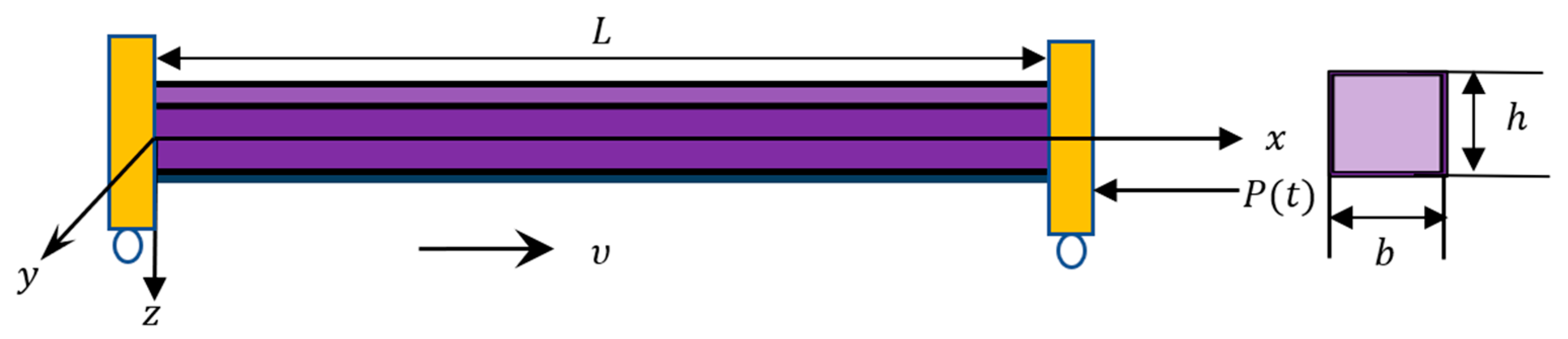
3. Problem Statement
A moving Euler–Bernoulli nanobeam, shown in
Figure 1, will be considered with length
and uniform cross-section
. To study the problem, a coordinate system
will be used, where the
-axis coincides with the central axis of the unqualified beam at first, and
is the neutral axis, while the axis
is the symmetry axis. The beam moves along its axis at a speed of
, and the beam is subject to an axial dynamic load. The bending stiffness of the beam is
, where
,
is the width, and
is the thickness.
In the theory of Bernoulli and Euler beams, the displacement components are addressed by [
44]
where
,
and
represent the components of displacement vector in
,
and
directions, respectively. It can be shown that
represents the beam’s deflection.
The following relations may be obtained using Equations (2), (3) and (10).
Substituting Equation (11) into Equations (1) and (4) yields
Following the Hamilton principle, the equation of the transverse vibration of the traveling nanobeam subjected to a longitudinal load
may be expressed as follows [
45,
46].
In this equation,
is the total bending moment. To calculate the resultant and a couple of moments (
and
), we use the given equations [
10,
17]:
Then, the total bending moment is given by
The nonlocal constitutive relations (7) of the Euler–Bernoulli nanostructure can be calculated as follows:
where
and
indicate the nonlocal thermal and couple stresses, respectively.
After applying Equations (14)–(17), the equation for total moment
, which is provided in Equation (11), is simplified to
Moreover,
stands for the thermal moment, which may be determined by the following relation.
Motion Equation (13) can be reformulated in its present form by substituting Equation (18) in Equation (13) to become
In addition, if we plug Equation (13) into Equation (18), we obtain the following.
If we substitute in the previous equations, we return the original local equation of motion for a moving Euler–Bernoulli beam.
By substituting Equation (10) into Equation (9), the following DPL heat transfer equation is obtained when no external heat source is present.
4. Analytical Solution
It will be considered that relationships
and
are fulfilled since heat is not transferred between the top and bottom of the nanobeam, which is isolated. Moreover, the nanoscale beam is skinny, and temperature changes (
) sinusoidally in the thickness direction (
). As a result, the temperature function can be written as the product of two functions: the first is
as a function of
in u only, and the second is a function
of axial distance
and time
as follows.
Equation (23) is substituted into Equations (20) and (21), and after some algebraic computations, we obtain the following:
where
.
Multiplying Equation (22) by
and integrating w.r. into variable
over the beam’s thickness from
to
leads to
We utilize the following non-dimensional variables to simplify the calculation:
where
and
.
In view of the use of Equation (27), Equations (24)–(26) can be presented in the following forms.
The primes have been excluded from the preceding equations for simplicity.
To find a solution to the problem at hand, it is necessary to take into account the starting conditions and limits. It will be assumed that all initial conditions in this scenario are homogeneous. The starting conditions will be as follows:
Moreover, the boundary conditions for the moving nanobeam are considered to be clamped at both edges. The following mechanical constraints may be considered in this case:
It will be assumed that the first edge of the beam (
) is thermally loaded, as in the following equation:
where
is a constant. It will be assumed that the load is a variable sinusoidal pulse function denoted by
. This assumption is capable of being mathematically represented as follows:
where
indicates the pulse width. Additionally, the other end of the beam (
) is supposed to be insulated. In this case, the thermal boundary condition can be written as follows:
In most of the previous literature, it was hypothesized that the axial force of transverse excitation was either non-existent or constant. The axial force is often variable with time as well as position. In the present work, it will be assumed that the dimensionless transverse axial tension will be a time-varying function as in the following relation [
47]:
where
is the loading frequency, and
and
represent the static and dynamic axial loads.
5. Solution Procedure
By using the initial condition from Equation (31) and the Laplace transform, the set containing Equations (28)–(30) can be simplified into the following set of equations:
where
Equations (37) and (38) can be doubled to obtain the following differential equation of the sixth order:
where
The expression representing the answer to Equation (41) can be expressed as follows:
where integral coefficients
and
were used, and constants
satisfy the following polynomial
Kulkarni [
48] developed a method for analyzing a six-degree polynomial problem into two cubic polynomials as components. Thus, the cubic polynomial is equal to zero and solved to give the six roots of the equivalent (44) in the roots. Importantly, when this method is used, the sum of the first three roots equals the sum of the last three roots. He established the prerequisites for the coefficients of such a solved equation.
Initially, the following polynomial will be taken into account:
In Equation (45),
,
,
,
,
, and
denote unknown coefficients in the component cubic and quadratic polynomials. If Equation (44), which can be written as Equation (45), can be factored into two cubic polynomial components, its solution is obtained. The following cubic equations are obtained by equating these polynomial components to zero:
The solution to the above issue consists of six cubic equations, each of which must be solved separately to obtain the six roots. Thus, in order to change Equation (44) into the form of Equation (46), the parameters of the two equations must be equivalent. This results in
All six roots of Equation (46) can be obtained by solving for the unknown parameters using the method shown above, which involves solving a cubic equation:
where
The compatibility between Equations (38) and (43) gives
With the help of the solution in (23), the expression for temperature
inside the converted domain can be found in the following form:
The axial displacement field can be produced after performing the Laplace transform and substituting Equation (43) in (6):
With the assistance of Equation (43), we can write the bending moment that is given in Equation (39) as follows:
Applying the Laplace transform to Equations (32)–(35), the boundary conditions of the problem can be expressed as follows:
Using the boundary conditions (54), we may solve for the functions of interest by substituting their solutions into the equations:
By solving this system of linear equations, we may determine the values of unknown coefficients , (). Here, the solution to the problem has been found in the Laplace transform field, and the system’s different areas have been postponed.
To obtain the expressions of the studied domain variables in the time domain, the Laplace transform of the transformed domains must be inverted. Obtaining these conversions may be a tedious and long process. In this case, we use approximate methods and numerical algorithms. In this denominator, the following Riemann sum approximation formula will be used to invert any function
in the Laplace domain to a function
in the time domain [
49]:
Many numerical tests prove that the value of must satisfy to obtain better accuracy in the rounding process. The software used for numerical calculations in this work is Mathematica.
6. Numerical Outcomes and Discussion
This section will compute and examine the numerical outcomes for the deflection,
; temperature change,
; flexural moment,
; and displacement
obtained in earlier sections of the paper. The modified couple stress (MCS) model will study the influences of parameters such as material length, nonlocality, time delay, and pulse width on field variables. While performing numerical calculations, the properties of the nickel (Ni) nanobeams will be taken into account and are as follows [
23]:
Calculations were performed to determine the numerical outcomes of non-dimensional thermo-physical fields, and the numerical values were generated based on the application of the non-dimensional physical parameters that were shown in Equation (29). All nanobeam lengths are taken to be dimensionless and will be given values of , , and . Additionally, the values of non-dimensional temporal parameters will be taken as , , and . Calculations and discussions are provided for three situations and examined in detail.
In the first scenario, we will look at how the behavior of thermophysical domains when the value of the dimensionless nonlocal parameter
is changed. These changes and numerical values will be represented in
Figure 2,
Figure 3,
Figure 4 and
Figure 5 in the case of applying the theory of couple stress (MCS). Two possible values of the nonlocal coefficient other than zero,
and
, will be taken into account for comparison and analysis. For the sake of comparison, it should be noted that the value of
represents the case of the local thermoelasticity model, which does not include the effect of a small length. Other non-zero values of this parameter refer to the nonlocal thermoelasticity theory. To obtain numerical results in this situation, it will be assumed that the pulse width parameter, as well as the phase delay parameters, and the axial velocity of the beam, are unchanged (
,
,
, and
).
From the graphs, it can be concluded that the impact of damping resulting from the nonlocal coefficient is remarkably prominent in all studied fields of physics. As the nonlocal factor is altered, the influence of responses on the beam may be observed more clearly. In addition, the effect of thermal vibration on the nanobeams becomes apparent when one of their edges is subjected to sinusoidally varying temperatures. In the same respect, the nonlocal properties of the nanobeams decrease with the increase in the nonlocal parameter of the nanobeam and vice versa. The study written in the literature [
50] agrees well with these results.
It should be noted that this model explains the effects of nonlocality within nanostructures. For this reason, the micro- and nanoscale properties of small-scale elastic materials are explained in two different ways by the MCS theory and the concept of nonlocal elasticity. As a result of this theory’s findings, different formulations of beams and structures that depend on their size have been made to accurately show how size affects them [
15]. As a result, there is an urgent need in the scientific community to simultaneously consider both physical explanations in order to create a more robust size-based model to predict the mechanical response of nanobeams that accounts for the effects of both softening and hardening stiffness.
Adding the idea of a nonlocal effect to the governing equations could lead to a decrease in stiffness, as shown in [
51], or an increase in stiffness, as shown in [
52]. According to [
53,
54], the current study discovers that as the value of the nonlocal constant increases, the flexural stiffness of moving nanobeams decreases dramatically.
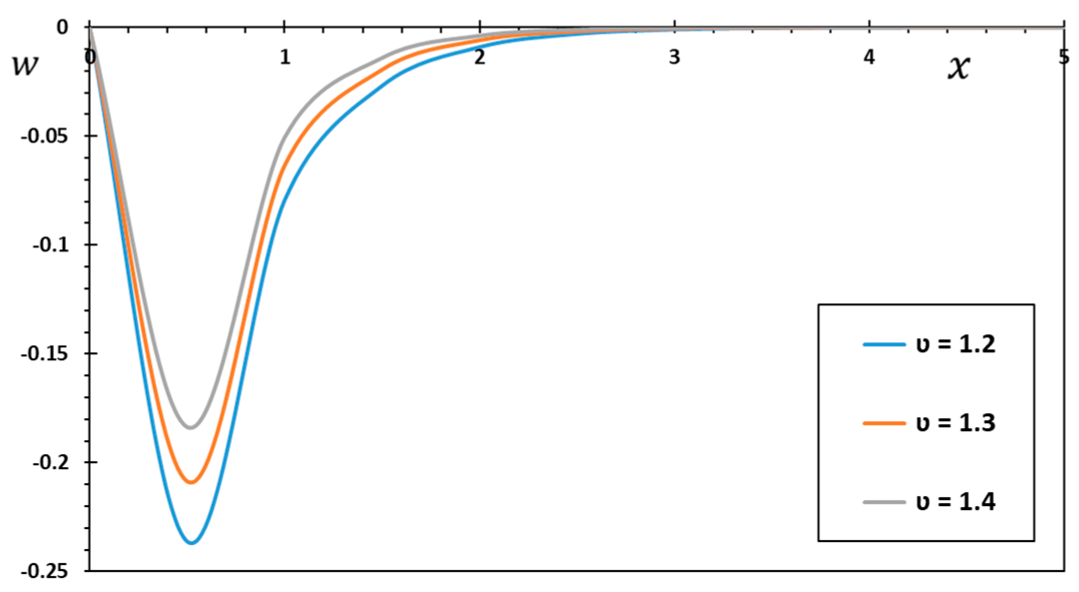
Figure 2 presents the variations in lateral deflection
of the nanobeam with changing axial distances. Based on the above, it is noted that the boundary conditions are met at both ends of the beam,
and
, where lateral deviation
begins and always ends at zero. This confirms the accuracy of the obtained results. On the other hand, it was discovered that lateral deviation
reaches its maximum value at a distance close to the edge of the first nanobeam and then decreases with the increase in length
. The reason for this is the presence of variable sinusoidal heating at that edge. It is noteworthy from the diagram that increasing the value of the nonlocal parameter causes deviation
to propagate slower and disappear more quickly. Nonlocal effects usually produce more pronounced vibration signals, unlike those obtained using the traditional vibrational notion.
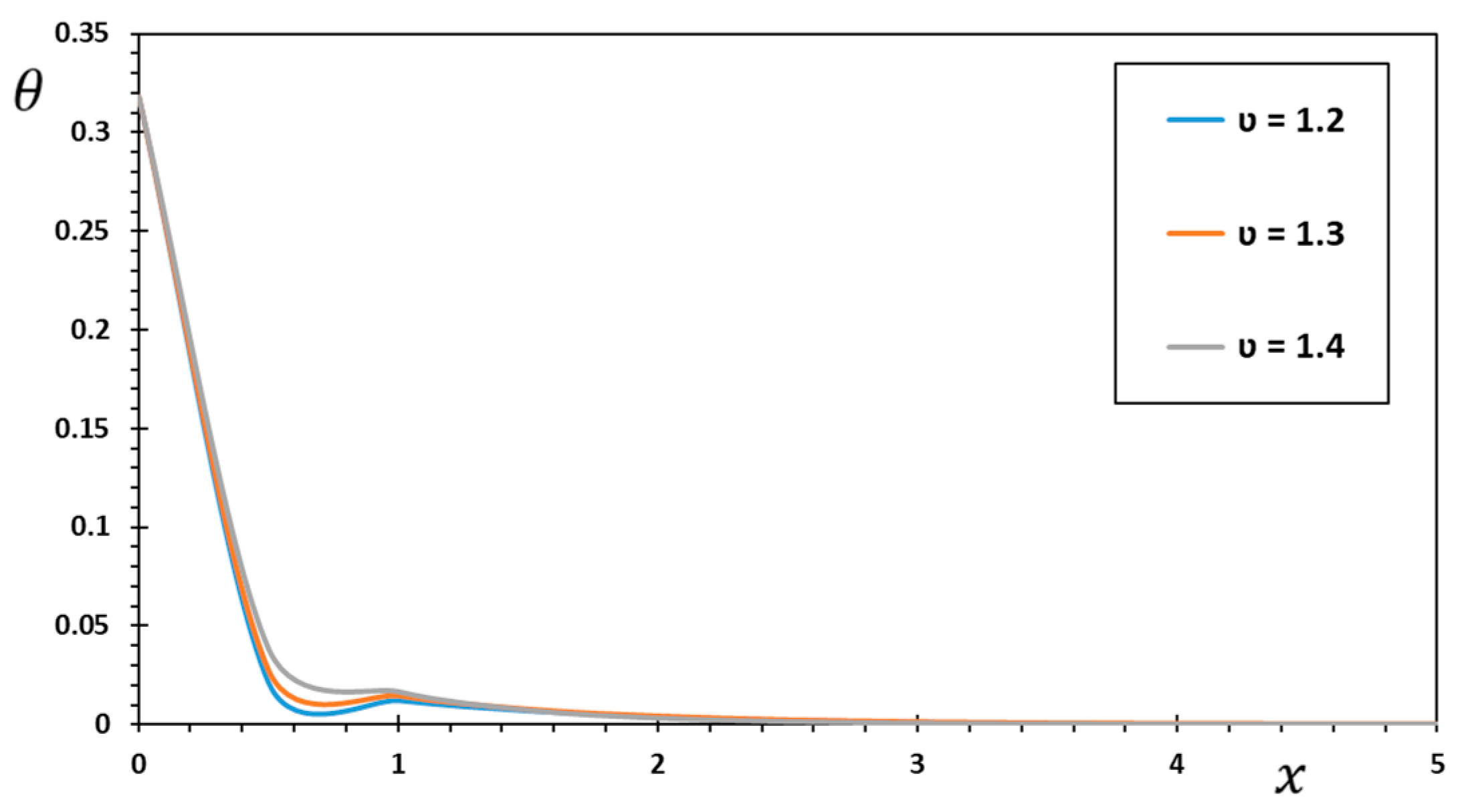
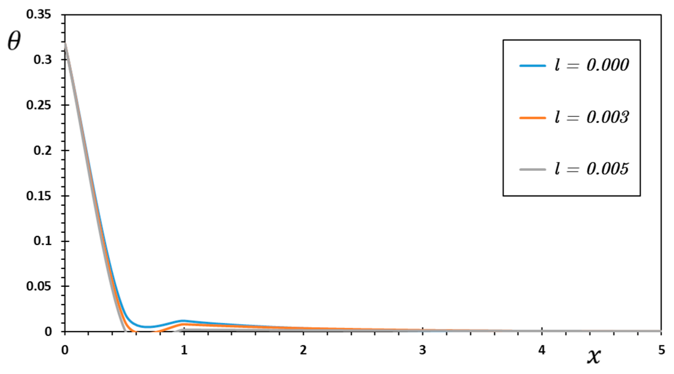
It is shown in
Figure 3 that changes in the values of nonlocal factors (
) have little effect on temperature profile
. This conclusion is consistent with many studies, as indicated in [
55,
56]. It is also clear from the diagram that as distance
increases in a direction opposite to the direction in which the heat wave travels away from the source, temperature decreases, which means that the spread of heat waves is limited. This observation contrasts with the traditional models of thermoelasticity, which predict infinite propagation speeds for thermal signals. On the other hand, these results confirm the importance of the proposed model in solving such physical conflicts.
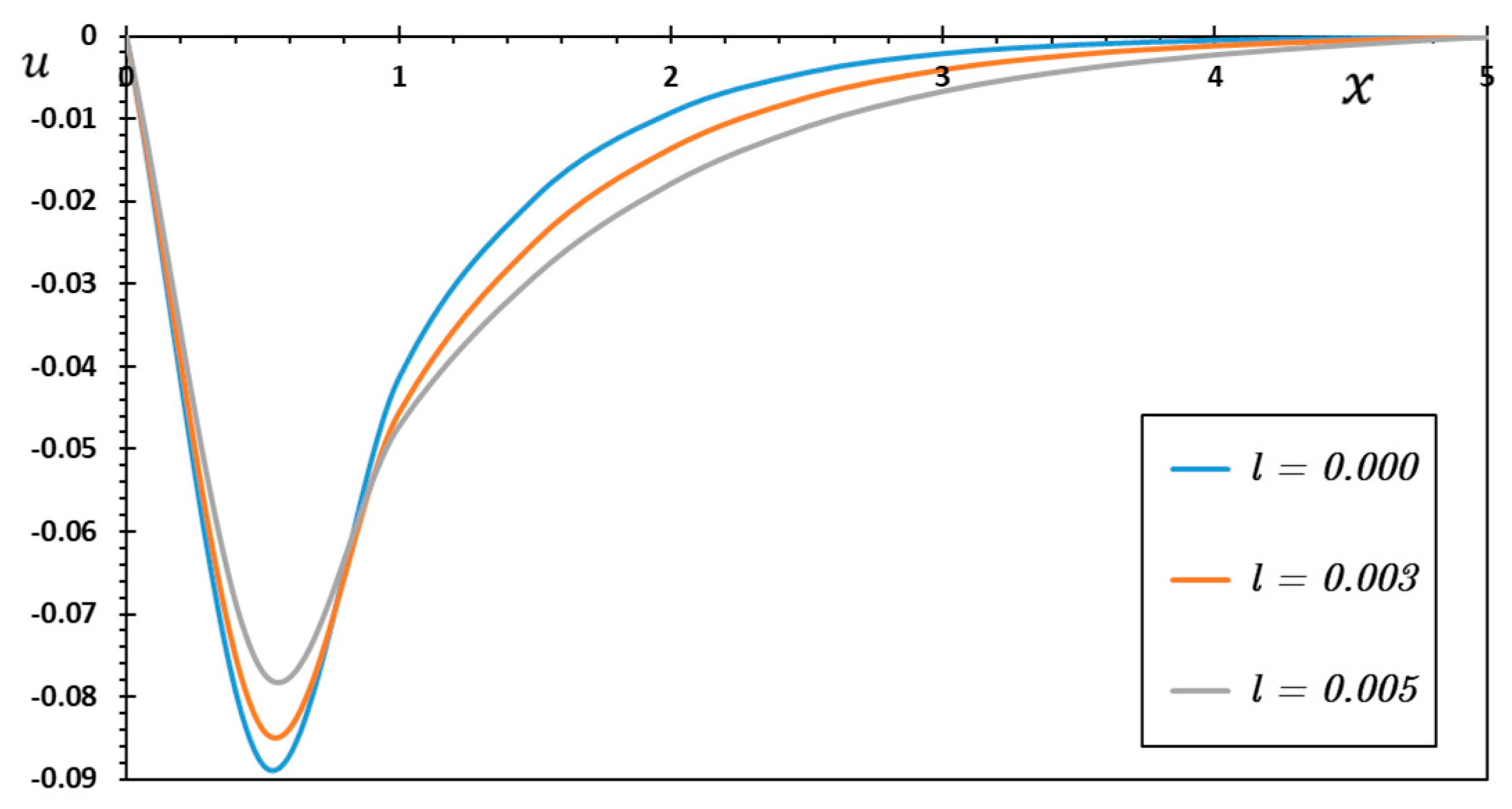
Figure 4 depicts the variations of the axial displacement
within the range of
at the instantaneous time,
, for different values of the nonlocal coefficient (
and
). In the schematic diagram, it is clear that displacement
starts with small values and increases rapidly to absolute values with an increasing beam length and then gradually decreases until it vanishes inside the medium. Notable in this figure is that deformation
was significantly affected by the nonlocal parameter change. It is observed that with increasing nonlocal values, distortion decreases. This is because the nonlocal indicator has a damping impact on the structure’s stiffness and is even more significant when employed to couple stress. Accordingly, a distinction must be made between local and nonlocal thermoelastic models in consideration.
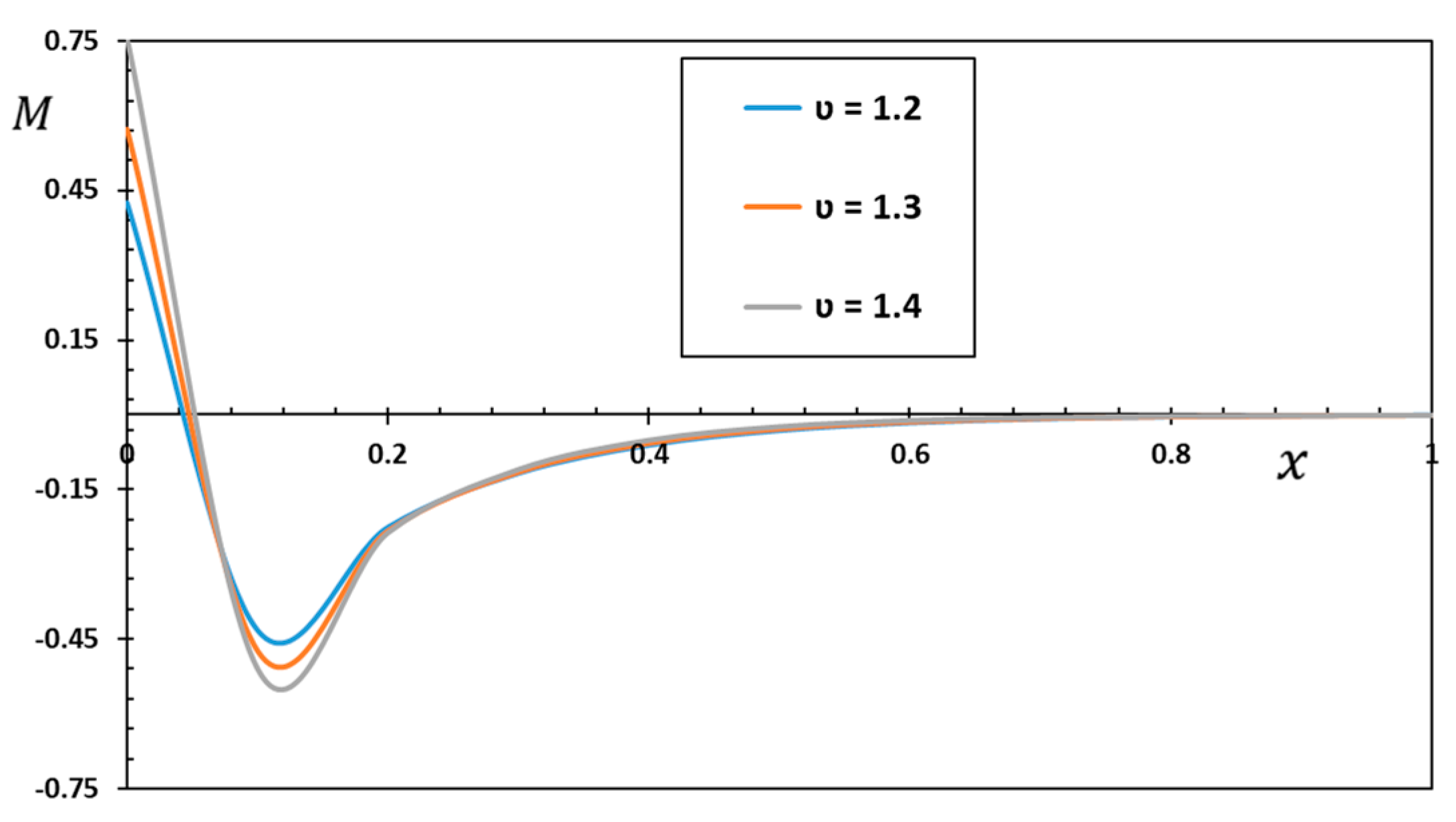
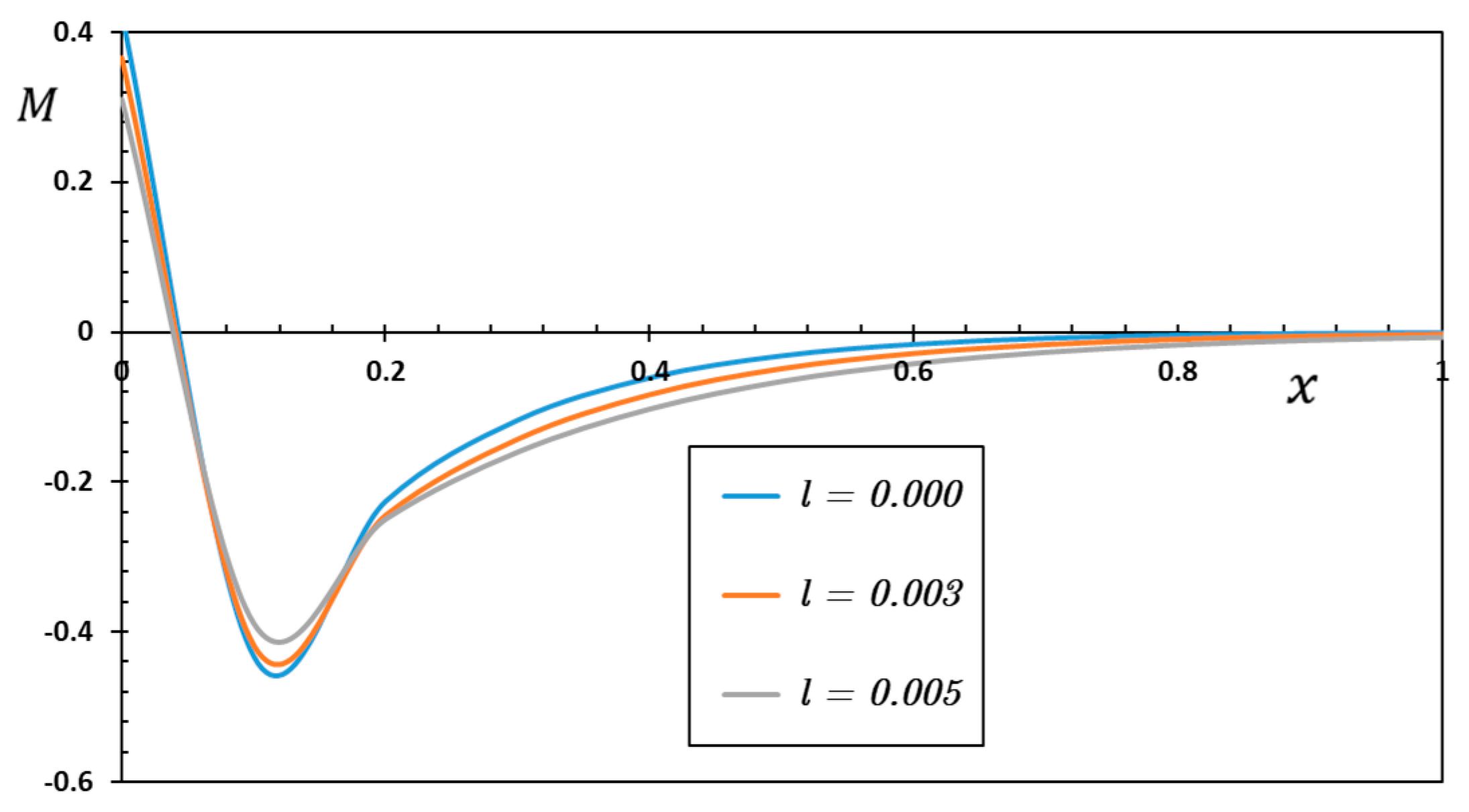
It can be observed in
Figure 5 how bending moment
changes with the variety of nonlocal parameter values and the change in distance. It can be observed from
Figure 5 that bending moment
starts with a value of zero at the first edge of the beam,
, increases to a constant maximum value at a distance close to it, and then gradually decreases to zero again. In
Figure 5, it can be observed that
is very sensitive to changes in the nonlocal parameter. This is due to the effect of hardening the stiffness of the length scale parameter, which corresponds with [
57]. Suppose one looks at the numerical numbers displayed in
Figure 5. In that case, one can see that the microstructure influence, here demonstrated by the couple stress effect, significantly increases the stiffness of the system, resulting in a significant reduction in bending moment
. This is why classical continuity models are insufficient for describing the patterns of microstructure behavior due to the lack of size-dependent variables. Nonclassical continuum models show that NEMS will have a particular set of physical properties and mechanical responses at the nanoscale and that minor effects in lattice dynamics are caused by the crystal’s structure [
58].
The second case from the discussion describes and analyzes how phase delays affect the change in the thermophysical fields under study. In this case, the other parameters are kept constant at
,
, and
.
Figure 6,
Figure 7,
Figure 8 and
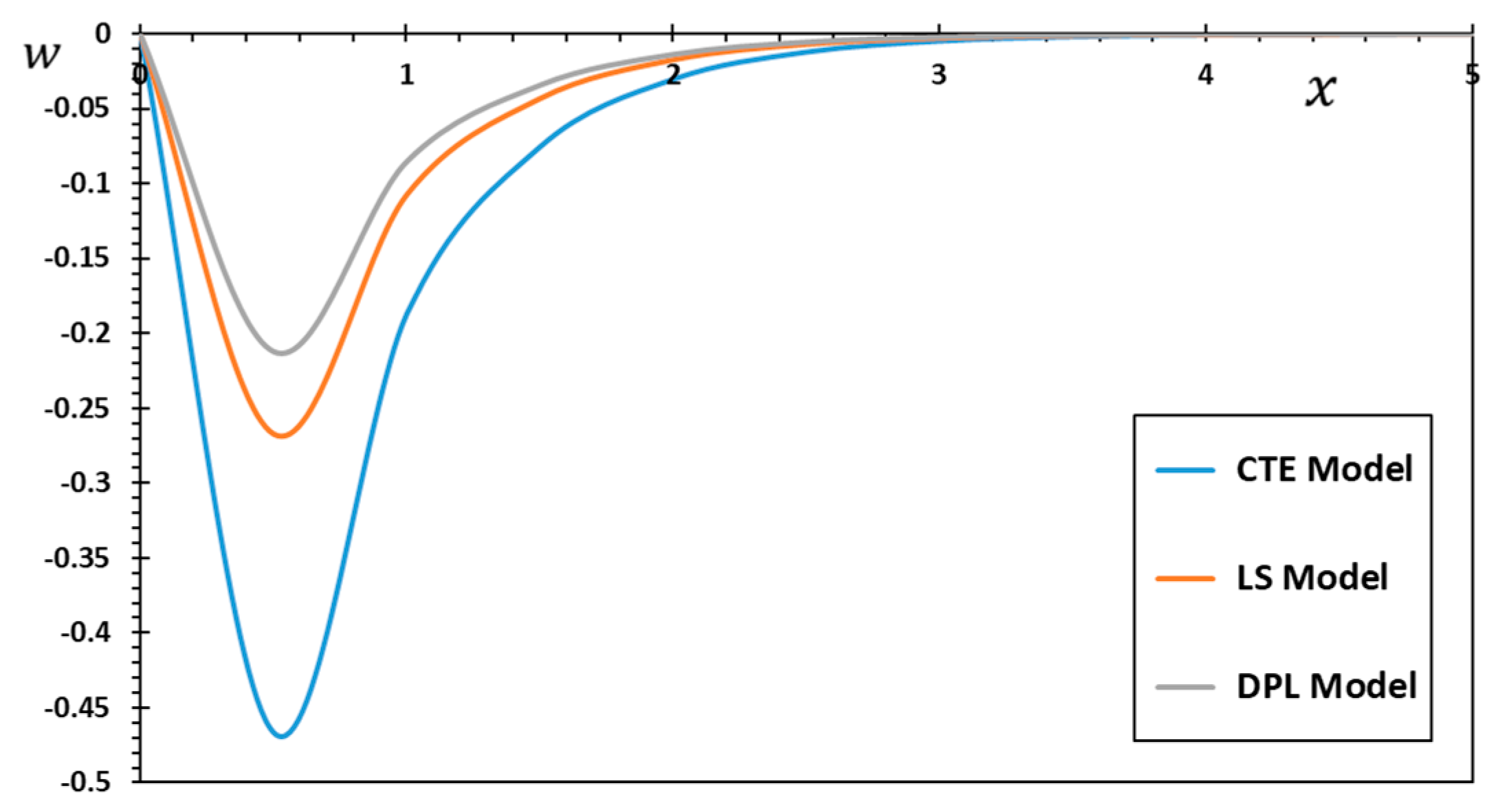
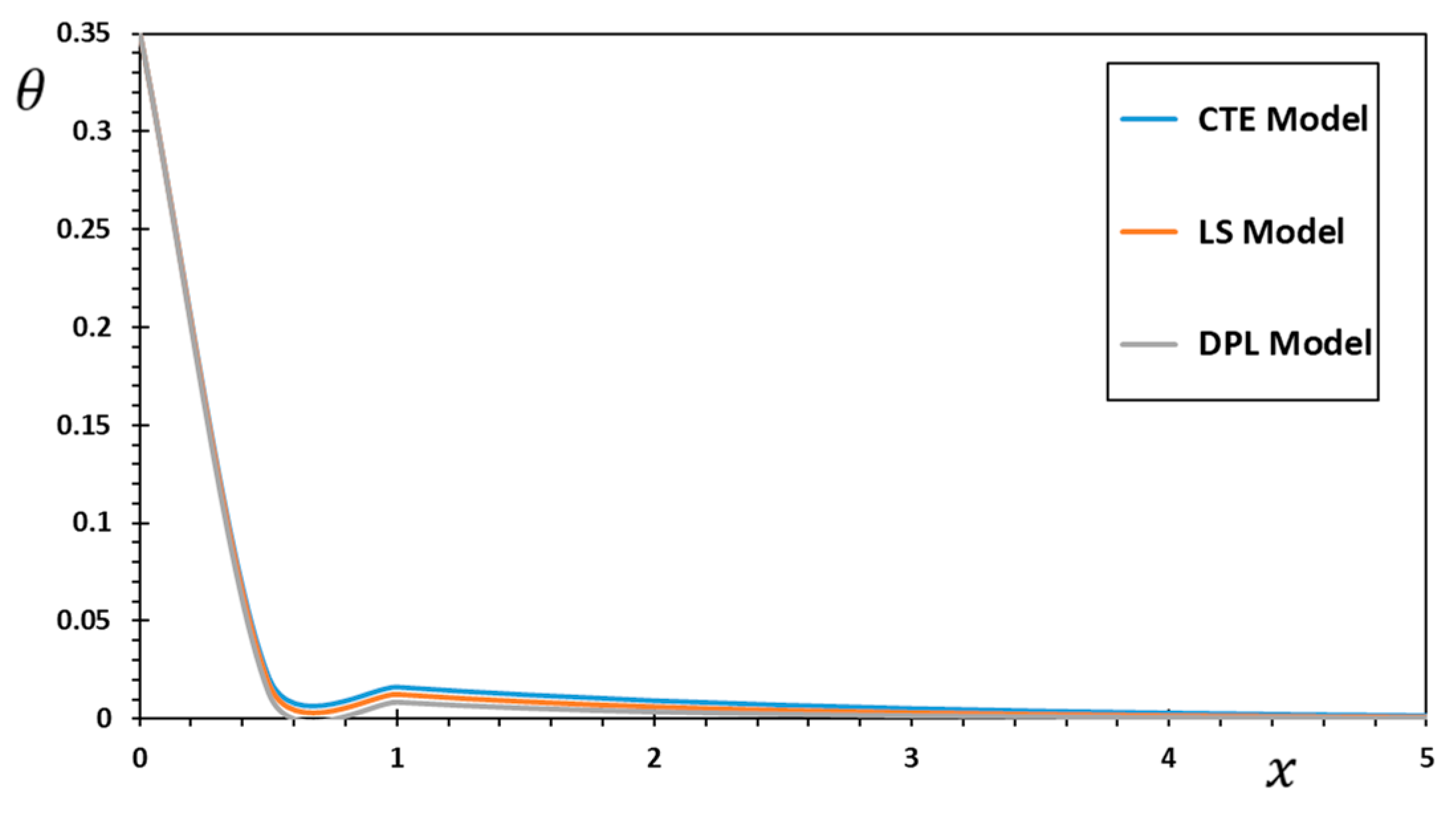
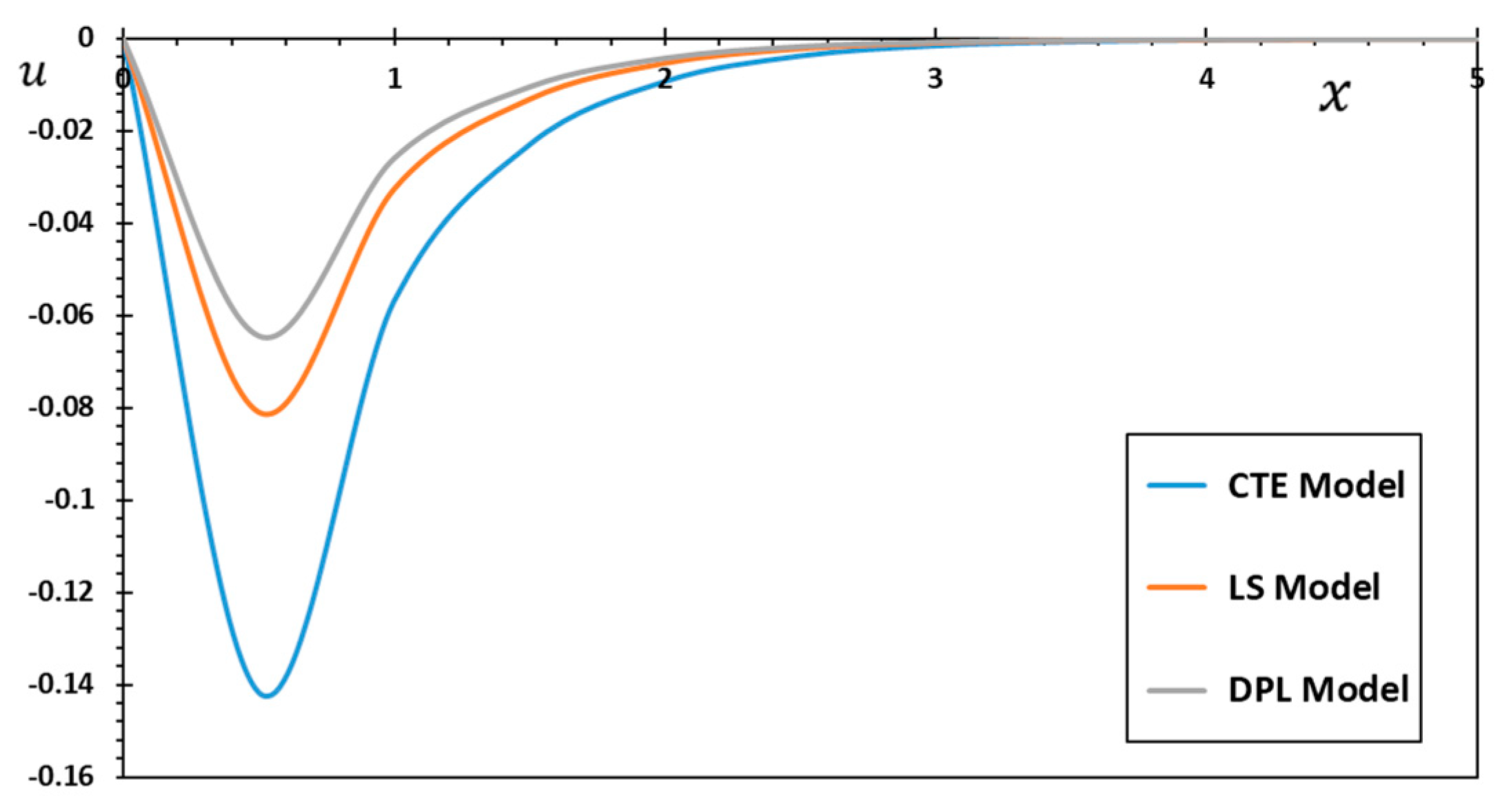
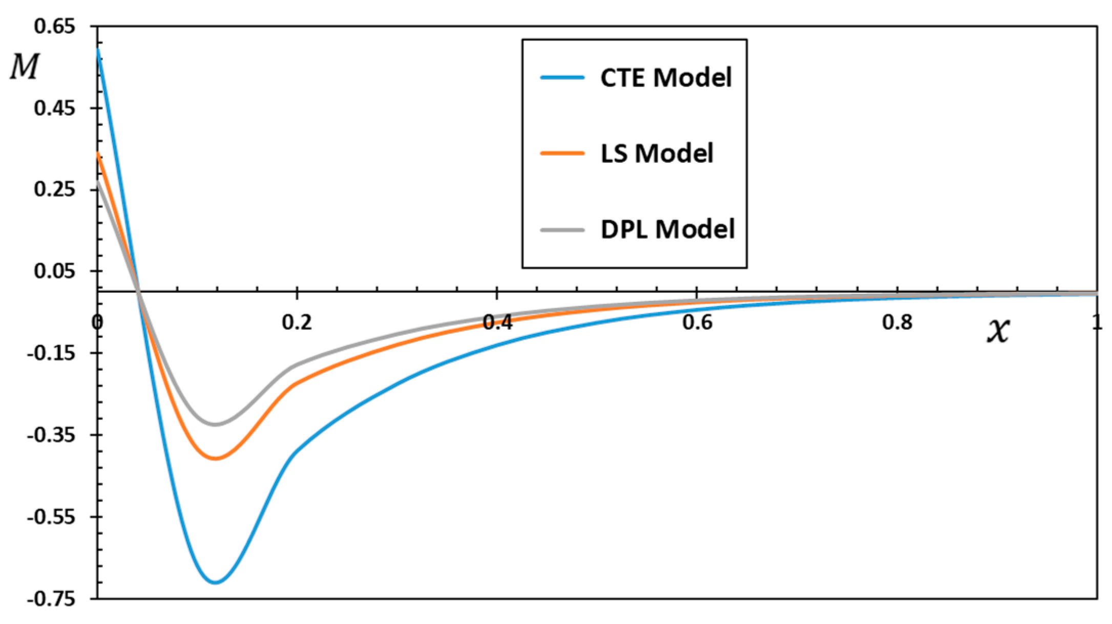
Figure 9 display the expected results for the system fields in the case of three different thermoelasticity theories derived from the suggested theory or that considered special examples of the current two-phase lag concept. The results of the conventional idea of thermoelasticity (CTE) can be obtained by setting
, while the predictions of Lord Shulman’s theory (LS) take
and
. Finally, in the case of Tzou’s extended theory of thermoelasticity, values
and
will be considered.
Figure 6,
Figure 7,
Figure 8 and
Figure 9 show how the behavior of the non-dimensional physical domains of the beam varies depending on the thermal model used. From the different shapes of curves, it can be observed that the phase delay factors (
and
) greatly affect how thermal physical quantities are distributed. The numerical results show that the classical thermoelastic model (CTE) has different values for the studied distributions than the other generalized thermal models. It also turns out that mechanical and thermal distributions do not disappear quickly inside the medium compared to other models. Extended theories of thermoelasticity were created to avoid the unrealistic physics predictions of the thermodynamic theory of thermoelasticity, according to which thermal signals move at an infinitely fast rate.
From the figures, it can be further concluded that the mechanical distributions move through the medium with a finite velocity according to the generalized thermoelastic theories (DPL and LS). Despite the difference in absolute values, most of the time, theories and models behave similarly. The results show that the theory of extended thermoelasticity is more in line with experimental findings for the material. The two-phase thermoelastic model also predicts that waves will travel at a limited rate within elastic media. It was further found that the heat flow phase delay and temperature gradient delay significantly affect the behavior of all domain variables. The presence of the temperature-gradient-induced heat flow phase delay, which is distinct from conventional Fourier diffusion, reduces the sharp wave velocity in the medium.
In the third case, the influences of the nanobeam’s axial velocity (
) on temperature change, flexural moment, axial displacement, and nonlocal thermal deflection are studied. In this case, different values of the axial velocities of the nanobeam (
, 1.3, and 1.4) will be taken when other effective physical parameters are fixed. The curves in
Figure 10,
Figure 11,
Figure 12 and
Figure 13 show how the axial velocity affects the moving nanobeams’ mechanical and thermal vibration properties. It is clear from the different figures that the mechanical fields, such as thermal deflection, axial deformation, and bending moment, increase with the increase in axial velocity while temperature decreases. From the different figures, it is clear how the changes in the behavior of the magnitudes of the fields correspond with the changes in the speed of movement (
) of the nanobeam and how these changes are susceptible.
The obtained results for a constant-velocity moving Euler–Bernoulli nanobeam and its corresponding results show good agreement with respect to behavior despite the different magnitudes. For example, when comparing the results of this work with those presented in references [
59,
60], it is possible to note the agreement between them. This behavioral agreement can confirm the current results’ validity and the proposed model’s accuracy. A sizeable transverse displacement may occur in the nanobeam under the action of axial velocity in a direction perpendicular to the speed, causing thermal and mechanical vibrations [
61]. As a result, unwanted noise can occur, limiting the structure’s ability to be used effectively, causing system stress, or driving a drop in quality. This is why such events must be considered in the industrial process to prevent stress or the performance degradation of the nanostructure due to deformations.
Because it does not consider small-size impacts, the traditional continuous theory of elasticity cannot describe dynamic vibrations in small beams and structures or predict how micromechanical systems with small dimensions will behave. In this last case of the discussion, the results of the modified couple stress model (MCS) will be compared with those of the conventional continuum theory. Comparing the couple stress theory with other classical models has two benefits. First, only one length scale parameter appears in the constituent equations. Secondly, the asymmetric bending and the pair stress tensor will be considered.
Figure 14,
Figure 15,
Figure 16 and
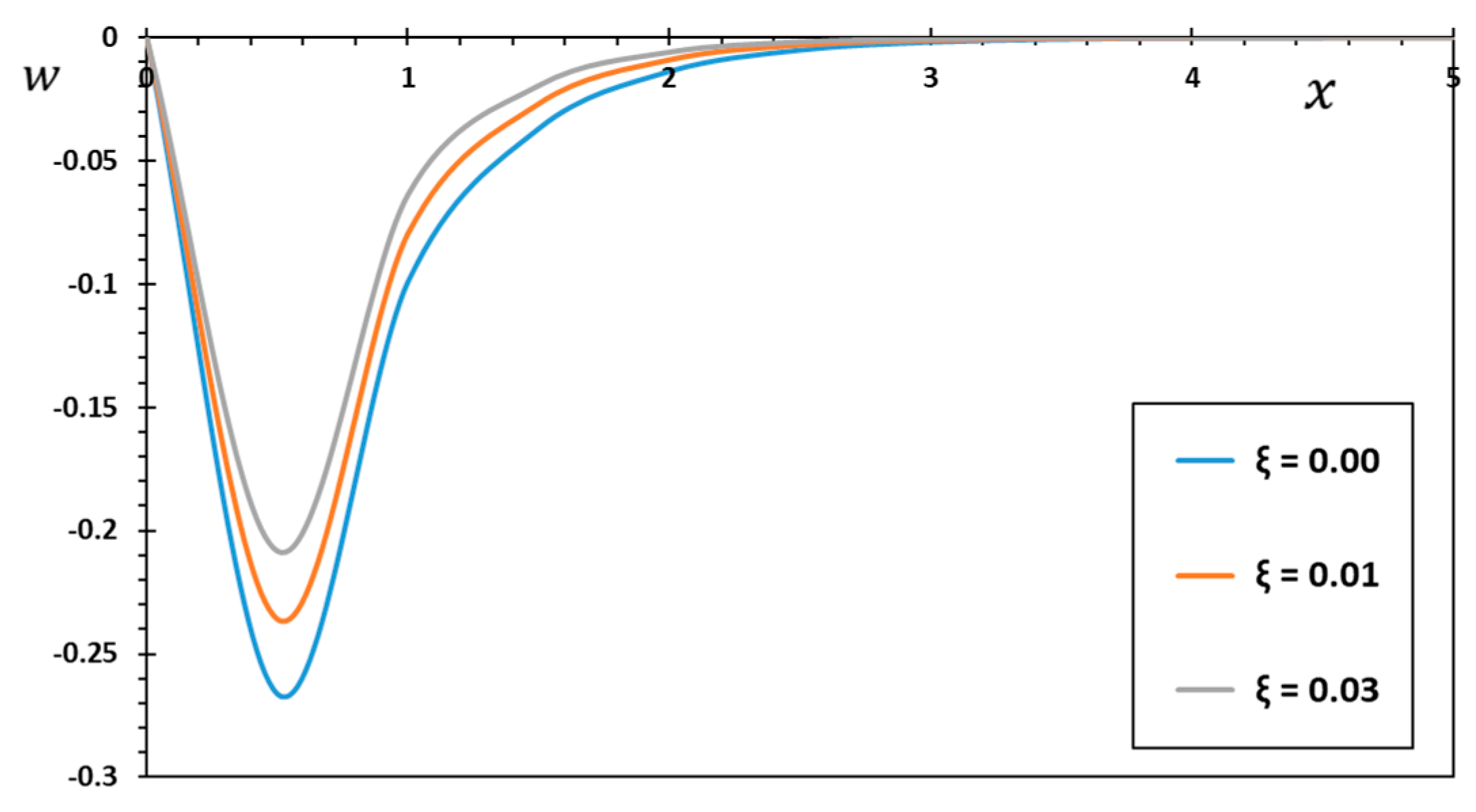
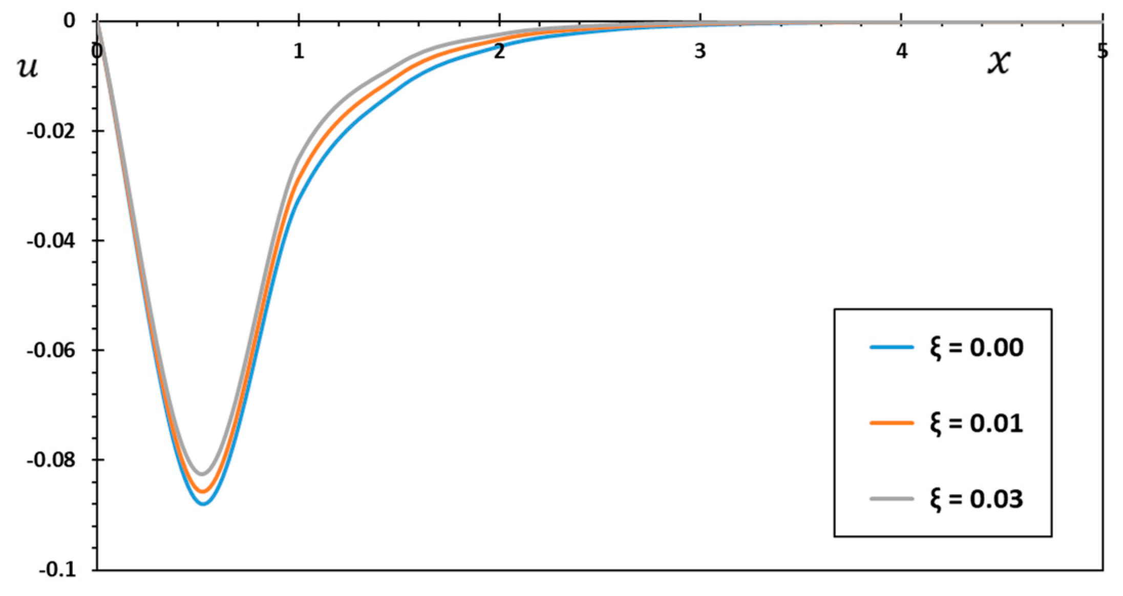
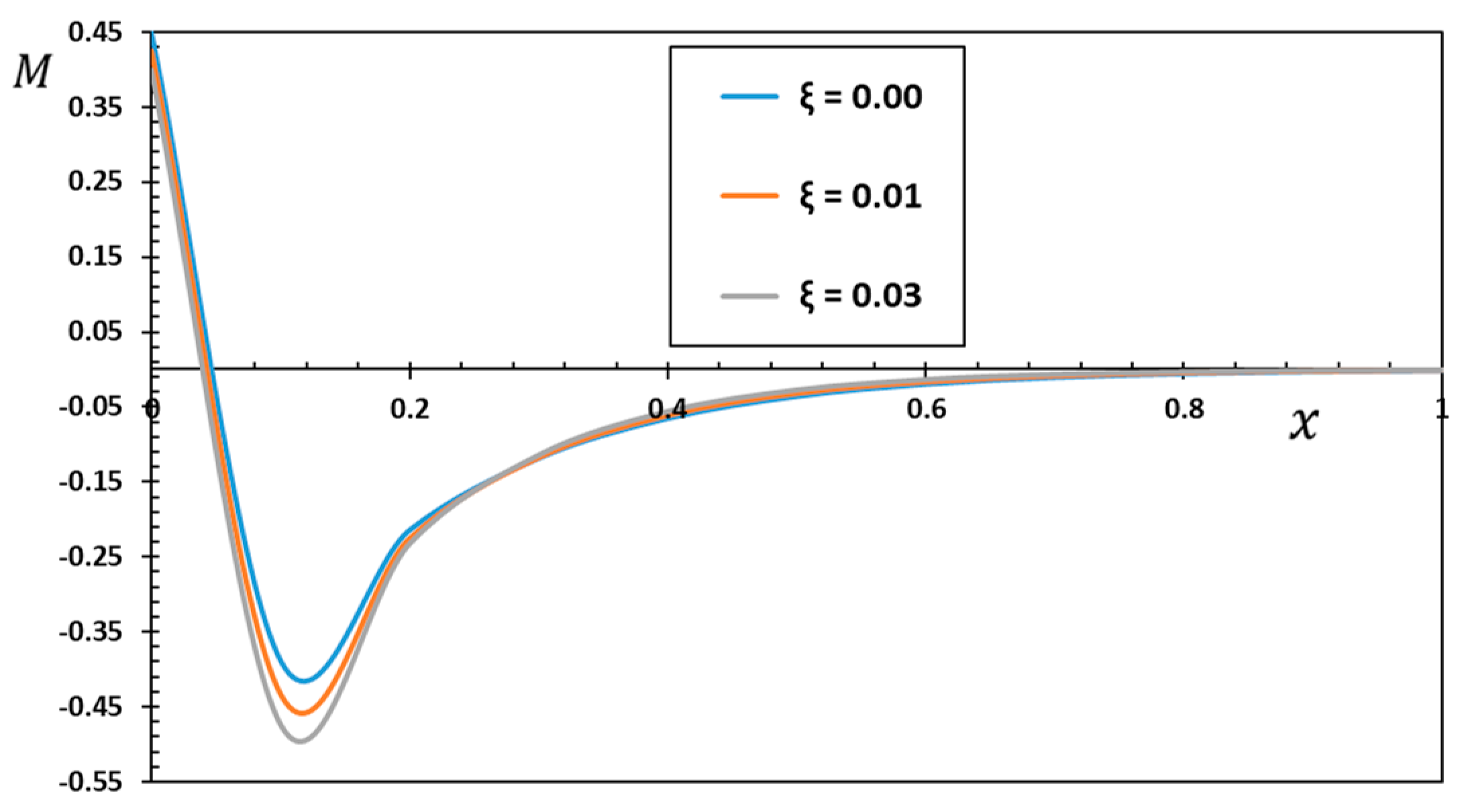
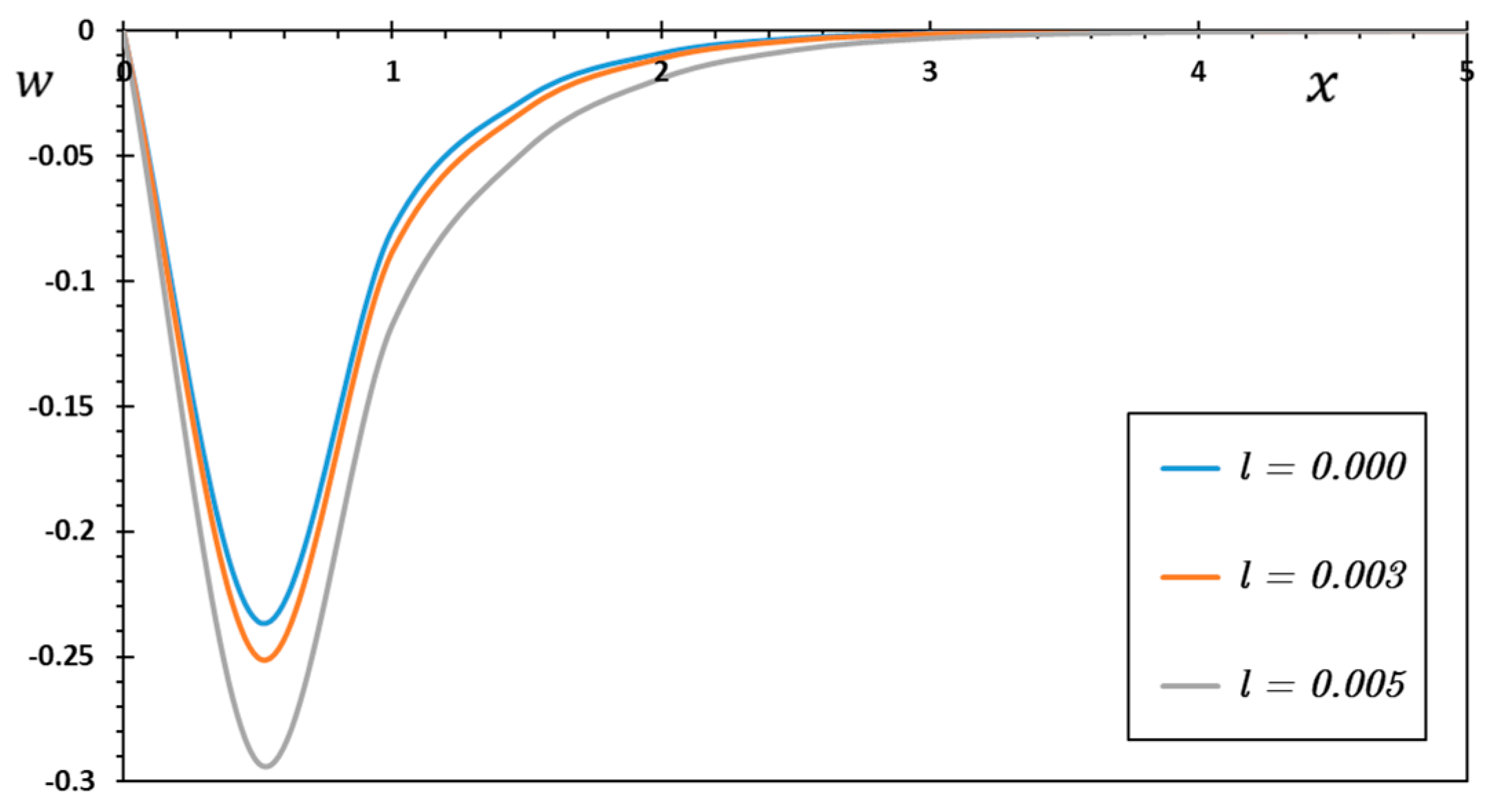
Figure 17 show the numerical results for domain variables under the MCS theory based on nonlocal Einstein elasticity. The results are then compared with each other and with the classical concept of continuum elasticity. The numerical results and graphs show how changing the material length scale parameter of the beam can change the patterns of entire physical fields and thermal and mechanical waves of the moving nanobeam.
Using the MCS concept, we obtain
when length scale index l is more significant than zero. Without the influence of the microscopic scale (
), we set
. Moreover, constants,
,
,
,
, and
are effective parameters. The domains taken into account are profoundly affected by the temporal scale parameter of the MCS theory. These results demonstrate that thinner nanobeams bend more severely than thicker ones due to the size effect. From the different forms of system domains, the numerical results in the MCS theory model show that the experimental values closely match. In contrast, Eringen’s nonlocal elasticity theory results are different [
62]. As a result, the dynamic and thermodynamic behaviors of micro- and nanobeams can be accurately modeled by the revised MCS theory [
2]. Additionally, from these illustrations, we can see that as the dimensionless length scale parameter increases, the size of the studied domains decreases, but it increases when the nonlocal parameter increases. The simulation results are in line with the pattern observed in refs. [
22,
63] and indicate that the smallest parameter value has the most significant impact on deformation and thermal deflection.
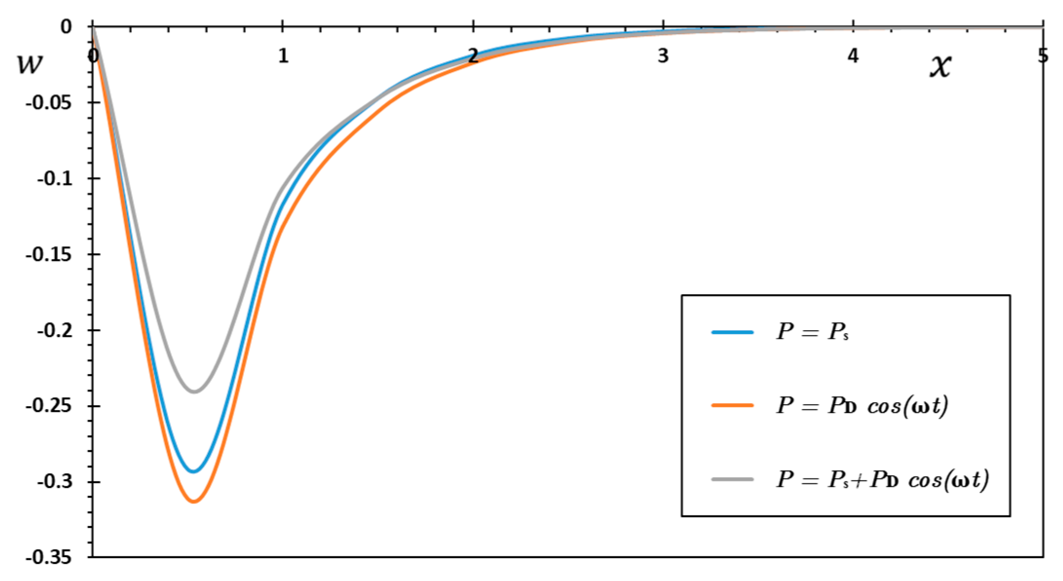
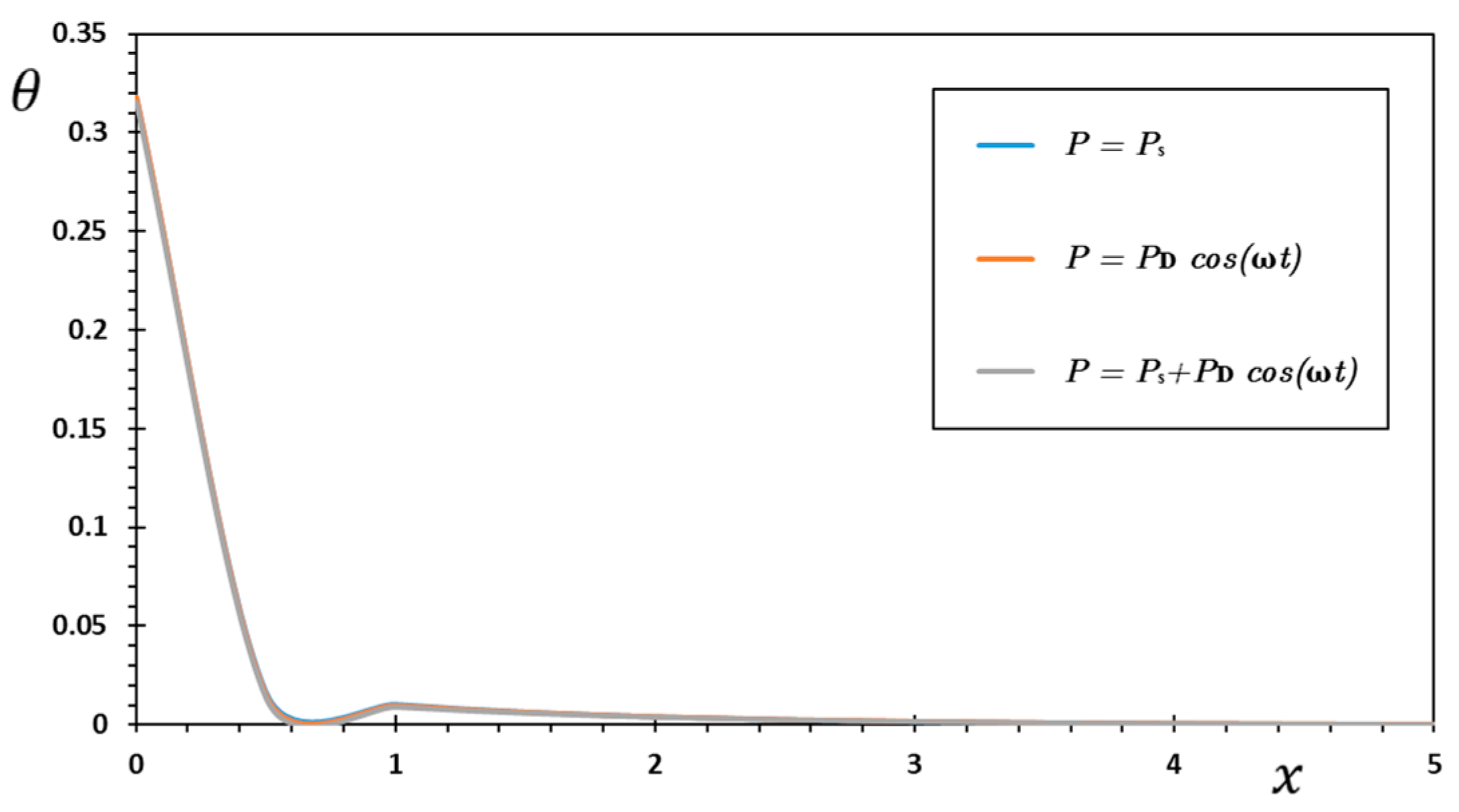
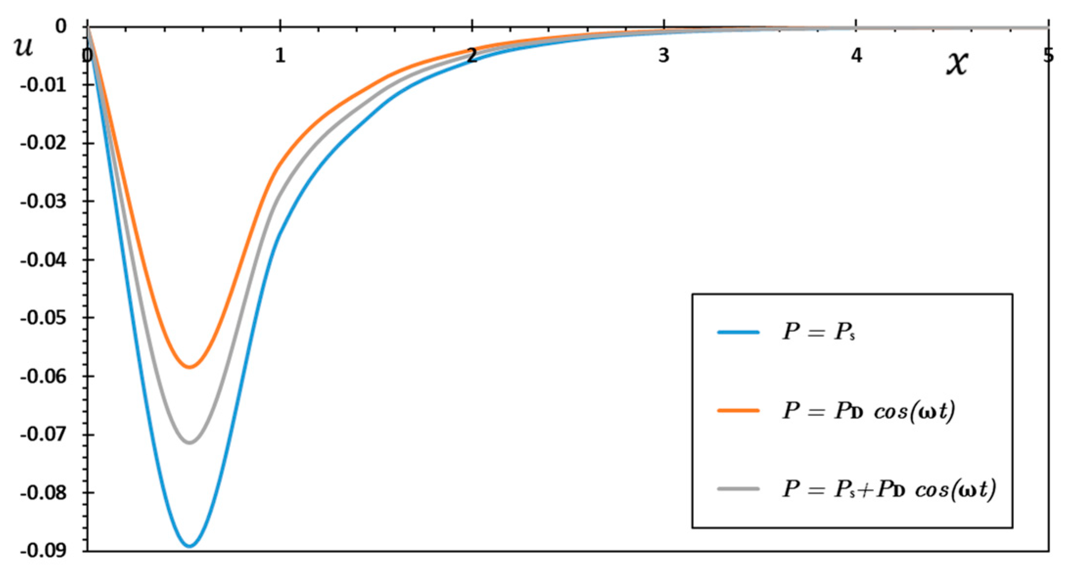
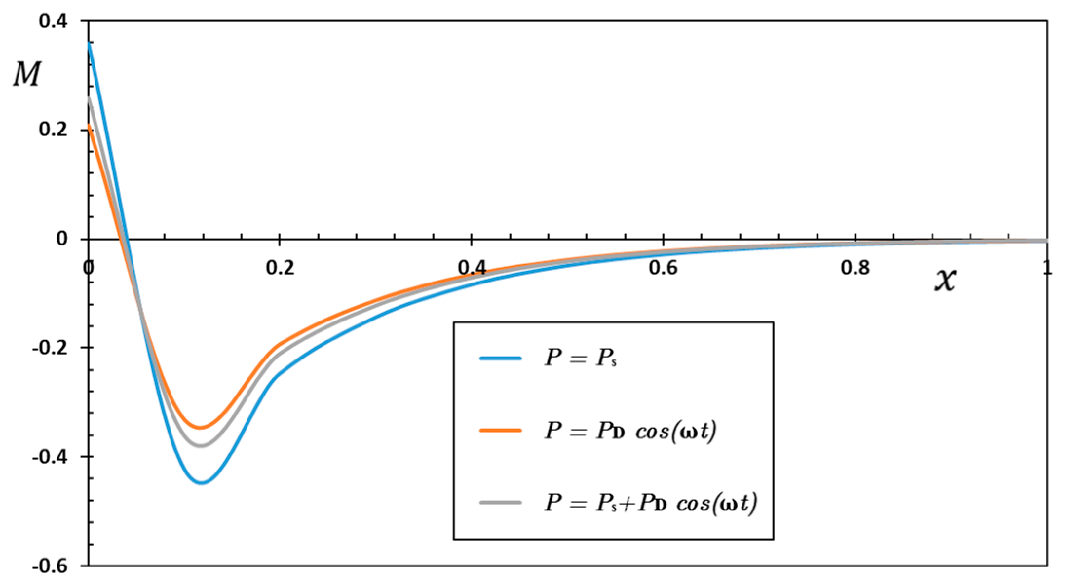
The thermodynamic stability studies of micro- or nanostructures subjected to time-dependent transverse external excitation are essential when researching the design and development of novel NEMS or MEMS devices.
Figure 18,
Figure 19,
Figure 20 and
Figure 21 show the effects of various transversal external stimuli on the group of studied physical fields. The responses of the checked domains will be validated by static (
), dynamic (
), and external transverse stimulation with amplitude (
). This part of the study will show how the axial tension force affects how the different domains in the moving nanobeam behave. Three other axial induction formula cases will be considered depending on the values of constants
and
: static, dynamic, or both.
In the different cases, the importance of axial force components and are considered, with the angular frequency of the applied transverse excitation remaining constant (). In this scenario, phase delay parameters and are assumed to remain constant along with nonlocal factor 1, axial motion velocity , pulse width , and other effective constants.
The graphs show how the axial tension force significantly affects different thermophysical fields’ behavior inside the nanobeam. Whether this external induction is static, dynamic, or both, it demonstrates the sensitivity of these fields to such changes. The curves of the analyzed fields display the same behavior in several scenarios to varying degrees. It is also evident from these graphs that the magnitudes of some areas increase under static external axial transverse excitation while others decrease with dynamic transverse excitation.


