Article

High-Enthalpy Geothermal Simulation with Continuous Localization in Physics

Faculty of Civil Engineering and Geosciences, Delft University of Technology, 2628 CN Delft, The Netherlands
*
Author to whom correspondence should be addressed.
Mathematics 2022, 10(22), 4328; https://doi.org/10.3390/math10224328
Submission received: 6 October 2022 / Revised: 12 November 2022 / Accepted: 16 November 2022 / Published: 18 November 2022

Abstract

:
Simulation of heat production in high-enthalpy geothermal systems is associated with a complex physical process in which cold water invades steam-saturated control volumes. The fully implicit, fully coupled numerical strategy is commonly adopted to solve the governing system composed of mass and energy conservation equations. A conventional nonlinear solver is generally challenged by the strong nonlinearity present during phase transition because of a huge contrast of thermodynamics between hot steam and cool water. In the process of solution, due to the steam condensation, the reduction in fluid volume reduces the pressure in the control volume. This generates multiple local minima in the physical parameter space, which indicates the Newton initial guess should be carefully selected to guarantee the nonlinear convergence. Otherwise, the Newton iteration will approach a local minimum and the solution based on Newton’s update cannot converge and needs to be repeated for a smaller timestep. This problem brings simulation to the stalling behavior where a nonlinear solver wastes a lot of computations and performs at a very small timestep. To tackle this problem, we formulated continuous localization of Newton’s method based on an Operator-Based Linearization (OBL) approach. In OBL, the physical space can be parameterized in terms of operators with supporting points at different levels of resolution. During the simulation, the operator values at supporting points are obtained through reference physics and the remaining part of the space is interpolated. In this way, the nonlinear physical parameter space can be flexibly characterized with different degrees of accuracy. In our proposed approach, the nonlinear Newton iterations are performed in parameter space with different resolutions from coarse to fine. Specifically, the Newton solution under coarser resolution is taken as the initial guess for that under finer resolution. A coarser parameter space represents more linear physics, under which the nonlinear solver quickly converges to a localized solution near the true solution. With refinement in physics, the Newton iteration will approach the true solution and the stalling behaviour in the simulation is avoided. Therefore, a larger timestep can be utilized in the simulation compared with the conventional nonlinear solvers.

1. Introduction

Against the background of global warming, geothermal energy [1], as a type of renewable energy, has been taken as an effective alternative for fossil fuels and utilized in power supply for decades [2,3]. During the development of geothermal reservoirs [4], the injected cold water will be heated by in situ fluid/rock and the heat can be carried up to the surface through water reinjection and cycling. For high-enthalpy geothermal systems [5], water can be present in the forms of vapor phase or vapor-liquid mixture under reservoir conditions. When developing the high-enthalpy geothermal reservoir with cold water injection, hot steam condensation happens after its contact with cold water. Therefore, multiphase flow and transport with phase changes appear in high-enthalpy geothermal systems.
Numerical simulation, as an efficient tool, can be used to model the mass and heat transfer processes happened in the subsurface reservoir. In geothermal simulation, the mass and energy conservation equations are usually tightly coupled since the fluid thermodynamics are functions of primary variables [6]. A fully coupled, fully implicit strategy is generally utilized in solving the coupled formulations. In a high-enthalpy geothermal simulation, numerical simulators can experience great difficulties, one of which is commonly known as ‘negative compressibility’. This problem was first described by Coats [7] with a single-cell numerical experiment, where a cell with saturated steam is invaded by cold water from the cell boundary with fixed pressure. Due to the invading of cold water, hot steam will condense, and the cell pressure will drop with steam shrinkage during phase transition. The cell pressure will constantly decrease until the steam is condensed and cell pressure then goes up to the injection pressure. To guarantee the convergence of a simulation, the timestep should be severely restricted which is often addressed as ‘stalling behavior’; see Pruess [8] for an example.
Pruess et al. [9] and Falta et al. [10] discussed the ‘negative compressibility’ problem. They concluded that the ‘negative compressibility’ effect is because of the idealization of complete thermodynamic equilibrium within the computational grids. Spurious pressure variation could occur in control volumes with the two-phase front because of the instantaneous thermodynamic equilibrium assumption, which will enforce severe limitations to the nonlinear convergence. Wang [11] made an analysis of the ‘negative compressibility’ problem in the fully implicit formulation. In that analysis, to ensure convergence of the fully implicit solution, a stability criterion for the timestep was developed and therefore, repeated timestep cuts were, to some extent, avoided. Nevertheless, the derived stability criterion is still quite restricted for simulations with larger timesteps. Wong et al. [12] applied a nonlinear preconditioner to the fully coupled, fully implicit solution. The formulations were first solved with a sequential fully implicit approach (SFI) and then the solutions were taken as the initial guess for the fully implicit method (FIM) [13]. Using this approach, the severe timestep restriction was reduced for some practical scenarios. However, there is still no robust strategy for converging a high-enthalpy nonlinear solution at a target timestep in the presence of the ‘negative compressibility’ phenomena. Therefore, it is of special interest to investigate an efficient way to tackle the issue of slow convergence appearing in the ‘negative compressibility’.
The partial differential equations included in a geothermal simulation are usually discretized within both spatial and temporal domains for approximate solutions. Generally, the governing system in discretized form has different degrees of nonlinearity and should be linearized. The discretized formulation is often linearized with a Newton-based procedure, where an assembly of the Jacobian matrix and residuals are needed. The values of fluid properties and their derivatives are involved in Jacobian assembly. With complex physical processes (i.e., multiphase compositional flow) involved in the setup, accurate physical properties should be evaluated through multiphase flash calculation [14]. This process is required to solve highly nonlinear local constraints in each Newton iteration for molar formulation [15]. Therefore, a heavy part of the overall simulation is occupied by the Jacobian assembly. Recently, the Operator-Based Linearization (OBL) approach was proposed by Voskov [16] to facilitate this process and therefore accelerate the linearization. Similar to discretization in spatial and temporal domains, the physics will be discretized within the domain of nonlinear unknowns in OBL.
In OBL, the governing equations are written in the form of operators with two categories: state-dependent and space-dependent. The state-dependent operators can be parameterized in physical space constructed by primary unknowns with different resolutions. The tables consist of pre-computed supporting points. By interpolation, the values and derivatives of the operators are evaluated with supporting points in parameter space. To further accelerate the linearization process, the adaptive parameterization technique has been proposed. In adaptive parameterization, operator values at the supporting points are evaluated along the simulation and stored for later reuse, which is especially efficient for parameterization in high-dimensional parameter space. In the meantime, it makes the Jacobian assembly simple and flexible even with complex physical processes. The OBL approach has been successfully utilized in simulating many kinds of physical processes in the subsurface [17]. The OBL technique also behaves as the underlying framework of the Delft Advanced Research Terra Simulator [18], whose robustness and efficiency have been sufficiently verified [19].
The OBL approach makes it possible to flexibly control the degree of physical nonlinearity by adjusting the resolution in parameter space. In other words, if fewer supporting points are chosen in parameter space, the nonlinear physics will become more linear, which makes it easier for the nonlinear solver to converge [16]. In this work, we follow the hierarchy of physical approximation in parameter space using the OBL formalism and construct a continuous solution in physics to solve the ‘negative compressibility’ problem. We start with general formulations and numerical strategies used in thermal-compositional simulations and briefly introduce the OBL approach. Next, the ‘negative compressibility’ problem in a single cell is described from the Newton path, residual distribution and operator surface. Afterward, the continuous localization in physics is adopted to solve the ‘negative compressibility’ problem. Finally, an idealized one-dimensional test case and a heterogeneous two-dimensional test case are used to verify the feasibility of the proposed method.

2. Methodology

During the production of a high-enthalpy geothermal reservoir containing aqueous phase, the mass and energy conservation equations are utilized to describe the governing system with two-phase thermal fluid flow and transport.
t ( ϕ j = 1 n p ρ j s j ) d i v j = 1 n p ρ j u j + j = 1 n p ρ j q j ˜ = 0 ,
t ( ϕ j = 1 n p ρ j s j U j + ( 1 ϕ ) U r ) d i v j = 1 n p h j ρ j u j + d i v ( κ T ) + j = 1 n p h j ρ j q j ˜ = 0 ,
where ϕ is reservoir porosity, ρ j refers to density of phase j , s j refers to saturation of phase j , U j refers to internal energy of phase j , U r is rock internal energy, h j is enthalpy of phase j , and κ is thermal conduction.
It is assumed that the fluid flow in the reservoir follows Darcy’s law,
u j = K k r j μ j ( p j γ j D ) ,
where u j refers to Darcy velocity, K is permeability tensor, k r j refers to relative permeability of phase j , μ j refers to viscosity of phase j , p j refers to pressure of phase j , γ j refers to specific weight of phase j and is defined as the product of the density of phase j and the gravity acceleration, and D is depth. In addition, to close the system, the summation of phase saturation should be equal to one,
j = 1 n p s j = 1
Next, Darcy’s law is substituted into the governing equation and the resulting nonlinear equations are discretized with a finite-volume method in space on a general unstructured mesh and with backward Euler approximation in time:
V [ ( ϕ j = 1 n p ρ j s j ) n + 1 ( ϕ j = 1 n p ρ j s j ) n ] Δ t l ( j = 1 n p ρ j l Γ j l Δ ψ l ) + Δ t j = 1 n p ρ j q j = 0
V ( ϕ j = 1 n p ρ j s j U j + ( 1 ϕ ) U r ) n + 1 ϕ j = 1 n p ρ j s j U j + ( 1 ϕ ) U r n Δ t l j = 1 n p h j l ρ j l Γ j l Δ ψ l + Γ c l Δ T l + Δ t j = 1 n p h j ρ j q j = 0
where V is the volume of the grid block and q j = q ˜ j V refers to the source and sink term of phase j . Δ ψ l is the phase pressure difference (including gravity and capillary pressure) between blocks connected via interface l , and Δ T l is a temperature difference between these neighboring blocks; Γ j l = Γ l k r j l / μ j l is cell transmissibility for phase j , and Γ l is the geometrical part of transmissibility, which is evaluated by the permeability and the geometry of the control volume. Γ c l = Γ l κ = ϕ ( j = 1 n p s j l λ j l κ r ) + κ r is the thermal transmissibility.
In the framework of molar formulation [12,20], pressure and enthalpy are selected as the primary variables for the nonlinear solution. In general, the Newton–Raphson method is used to solve a linearized system of equations in each nonlinear iteration in the following form:
J ( ω k ) ( ω k + 1 ω k ) + r ( ω k ) = 0
where J refers to the Jacobian matrix constructed within the k th nonlinear iteration. In the traditional method, the assembly of a Jacobian matrix requires accurate evaluation of the values and derivatives of physical properties. During this process, either different sets of interpolations (for properties such as relative permeabilities) or solution of a highly nonlinear system (e.g., multiphase flash) is needed. To meet the convergence requirement, the nonlinear solver has to undertake many iterations to resolve the minor variations in properties, which are sometimes unnecessary because of the numerical nature and uncertainties of physical properties. The Operator-Based Linearization approach, described below, is proposed to resolve this issue.

3. Operator-Based Linearization (OBL) Approach

The mass and energy conservation equations, in the OBL approach, are distinguished as different types of operators, the state-dependent and space-dependent operators. By name it can be recognized that the state-dependent operators are functions of a physical state ω , whereas the space-dependent operators are correlated as functions of a physical state   ω and a spatial coordinate ξ [16,21]. Pressure and enthalpy are selected as the primary state variables in geothermal simulations.
The discretized governing equation of mass in operator form is expressed as:
a ( ξ , ω ) ( α ( ω ) α ( ω n ) ) + l b ( ξ , ω ) β ( ω ) + θ ( ξ , ω , u ) = 0
a ( ξ , ω ) = ϕ V
α ( ω ) = j = 1 n p ρ j s j
  b ( ξ , ω ) =   Δ t Γ l ( p b p a )  
β ( ω ) = j = 1 n p ρ j l k r j l μ j l
where α ( ω ) 
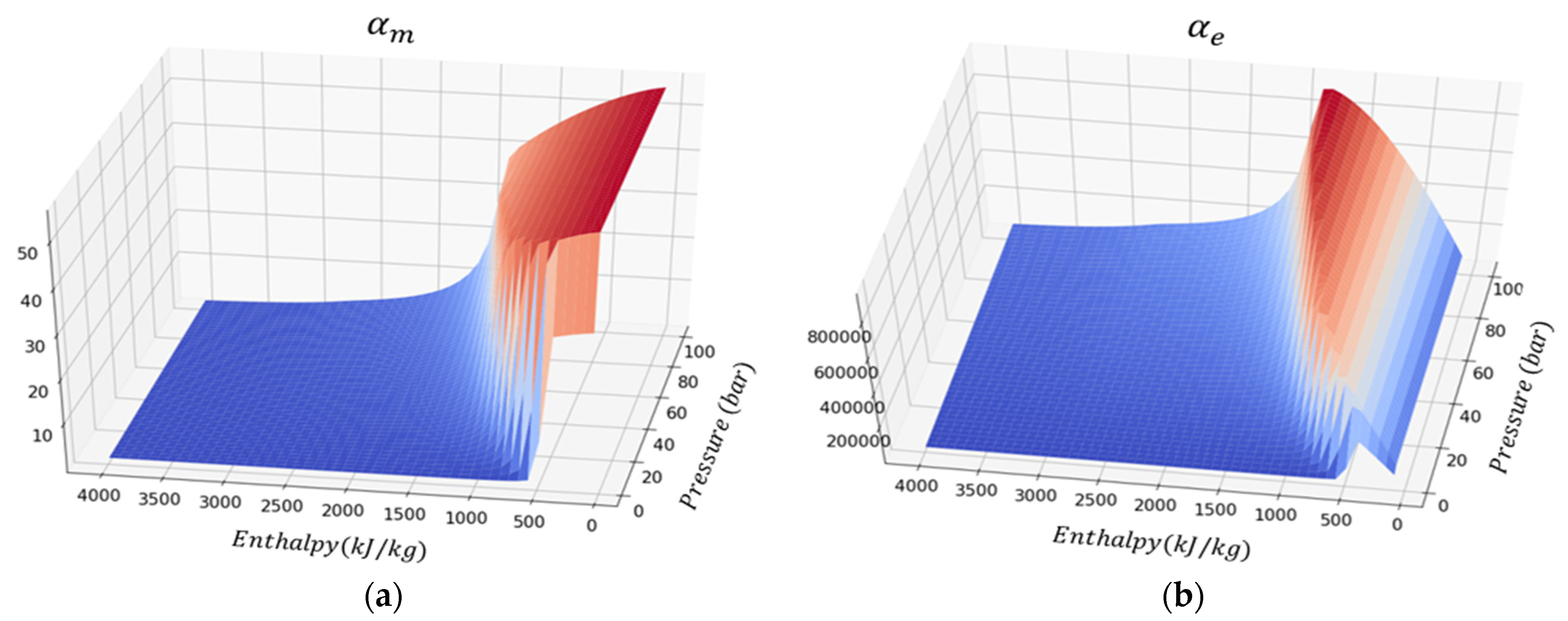
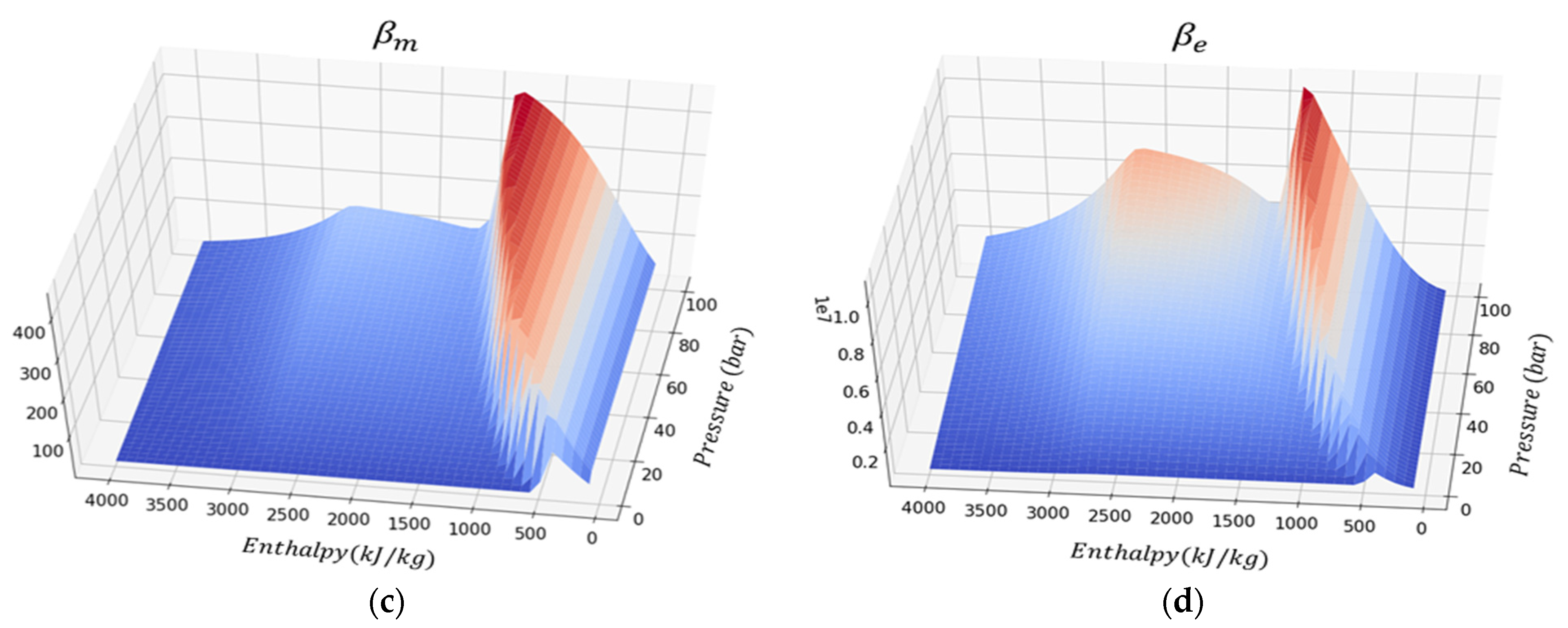
is defined as the mass accumulation operator, and β ( ω ) is called the mass flux operator.
The discretized governing equation of energy in operator form is expressed as follows:
a e ( ξ , ω ) ( α e ( ω ) α e ( ω n ) ) + l b e ( ξ , ω ) β e ( ω ) + l c e ( ξ , ω ) γ e ( ω ) + θ e ( ξ , ω , u ) = 0 ;
a e ( ξ ) = V ( ξ )
α e ( ω ) = ϕ ( j = 1 n p ρ j s j U j U r ) + U r  
b e ( ξ , ω ) = b ( ξ , ω )  
β e ( ω ) = j = 1 n p h j l ρ j l k r j l μ j l
c e ( ξ ) =   Δ t Γ l ( T b T a )
γ e ( ω ) = ϕ ( j = 1 n p s j λ j κ r ) + κ r
where α e ( ω ) is defined as the energy accumulation operator, and β ( ω ) is called the energy flux operator. This representation in operator form will be used to significantly simplify the general-purpose simulation framework. Without conducting complicated estimations of the value and derivatives of each property during the simulation, we can parameterize the state-dependent operators in the space of unknowns with a limited number of supporting points and use multilinear interpolation to evaluate them [16]. This not only makes the Jacobian assembly simpler but also improves the simulation performance since almost all expensive property evaluations are replaced by interpolations. In addition, due to the piece-wise multilinear approximation of physical operators, the system will become more linear and the performance of the nonlinear solver can be improved.

4. Single-Cell Problem with ‘Negative Compressibility’

4.1. Formulations

The ‘negative compressibility’ problem can be described using a single-cell model with a cold water injection at a fixed pressure [7,22]. To facilitate the description, the following assumptions are made:
1.
Neglect the rock energy;
2.
Heat conduction is ignored;
3.
Rock is incompressible.
Therefore, we get the following mass and energy conservation equations for a single cell problem:
V ρ t t Υ ( p i n p ) = 0 ,
V ρ t h t H i n Υ ( p i n p ) = 0 ,
ρ t = ρ w s w + ρ s s s ,
where Υ refers to the flow transmissibility at the injection boundary, p i n refers to the fixed pressure of the injection boundary, p is the pressure of the cell, h is the enthalpy of the cell, ρ t is the total fluid density, ρ w , ρ s are the density of water and steam, respectively, and s w , s s are the enthalpy of water and steam, respectively. In the following, we take a single cell example to illustrate this problem with p = 50   bar , h = 2000   kJ / kg , s s = 0.97 and p i n = 90   bar , H i n = 345   kJ / kg .

4.2. Newton Path

Wong et al. [22] derived and distinguished the timestep for the Newton solution to converge based on the pressure solution of the Newton update. Here, we take the timestep that forces the Newton solution to diverge. Figure 1 shows the Newton path starting with an initial guess chosen to be identical to the initial condition. Because of the large variations in thermodynamic properties between water and the steam phase, the residual equation becomes highly nonlinear. In Figure 1, one can recognize two minima in the residual map: one (in the upper right part) is the local minimum which does not correspond with the solution (here residual is not equal to zero); the other one (in the lower middle part) is the real solution of the problem. If the Newton update follows the gradient of the residual equation starting with the proposed initial guess, it will converge to the wrong local minimum. Notice that in conventional nonlinear solvers, the solution at the previous timestep is taken as the initial guess for the Newton method which can be any point in parameter space. To check how convergence for a given set of parameters depends on the initial guess, we chose uniformly distributed points within pressure-enthalpy space and checked convergence for all of them respectively. The convergence map is shown in Figure 2.
It is clear from Figure 2 that the Newton path starting with points in the two-phase region (upper part of the residual map) will either diverge or converge to the local minimum; whereas for the points in the single-phase region, the Newton iterations will converge to the real solution. As shown in the results, if the initial guess is in the two-phase region, the simulation at this timestep will waste several nonlinear iterations and finally cut the current timestep (with possible further timestep cutting in following iterations). This indicates that finding a suitable initial guess for Newton iterations is essential to guarantee the performance at a targeted timestep in a geothermal simulation with steam condensation.

4.3. Operators

In Figure 3, the operators for mass and energy conservation equations are plotted with fine resolution tables. Here, α m and β m correspond to the accumulation and flux terms in Equation (7) for mass, and α e and β e correspond to the accumulation and flux terms in Equation (9) for energy. As you can see, all operators are highly nonlinear in pressure-enthalpy parameter space. If the initial guess is in the two-phase region, the Newton process cannot jump across the phase boundary and stay on the wrong side. This gives further evidence of the fact that the nonlinear solver struggles in the high-enthalpy geothermal simulation.

5. Continuous Localization in Physics

Through the analyses above, we notice the high nonlinearity in physics causes difficulties for the gradient-based nonlinear solver and forces it to update in the wrong direction. This inspires our approach with a multi-level physics parameterization taking advantage of the unique feature of the OBL approach, which enables us to define parameters in the physical space with different levels of resolution according to custom requirements.

5.1. Continuous Localization of the Newton Iteration

The continuous localization of the Newton iteration aims to find a good initial guess for the nonlinear solution under a reference physical resolution. The logic of the localization is illustrated as follows.
Instead of solving the system with reference physics at the very beginning, we start the simulation for a targeted timestep with a coarse OBL parameterization, which was prepared through pre-experiments in advance. The pre-experiments are necessary and helpful in determining the number of levels during the localization stage. Because of the coarse resolution of the parameter space, the Newton residual map will change from that under the reference resolution, and becomes almost linear with a monotonically behaving residual (see Figure 4a as an illustration). This means that only a few iterations are needed to reach the solution under this coarse physical resolution. Therefore, the nonlinear solving procedure is largely facilitated by the coarse parameterization. Notice that even though the solution at this stage is different from the final solution, it has brought the initial guess (generally the solution of the last timestep) to the vicinity of the true solution, which will be observed from Figure 4c.
With the solution from a coarse resolution as the initial guess, a fresh Newton iteration is performed with a refined physical parameter space. The objective of this step is to build a smooth transition from the solution under a coarse resolution to that under a refined one and guide the localized solution closer to the real (reference) solution. As is shown in Figure 4b, this step helps to localize and direct the Newton update in the right direction. Also notice that the full residual already behaves non-monotonically and there is a region in parameter space with a wrong gradient (in the upper-right part). However, the localization stage at a previous coarser level helps to safeguard the Newton update in moving towards the true solution. Because the nonlinearity of physics under a coarse resolution and the reference resolution can be distinguished, this necessary step bridges the nonlinear updates across different resolutions.
Finally, the reference resolution is used to perform nonlinear iterations with the previous localized solutions as the initial guess. This step is to ensure the targeted nonlinear problem is accurately solved. Even though the residual is non-monotone at the reference resolution and a large region of the parameter space has the wrong gradient (see Figure 4c), the localized solution at previous OBL resolutions still provides a good initial guess to safeguard the Newton update in pointing to the true solution.
The flowchart of the continuous localization of the Newton iterations is displayed in Figure 5. The localization stages may include several updates under different physical resolutions based on the specific initial and injection conditions of the problems being solved. The essence of these multi-level nonlinear updates is to provide a good localized initial guess for the later nonlinear iteration under reference resolution, and therefore help the convergence of the nonlinear solver.

5.2. Convergence Analysis

To verify the feasibility of our approach for different initial guesses, we choose various points uniformly distributed in the parameter space, and the results of the Newton convergence are shown in Figure 6. It is obvious that any initial guess in the parameter space will first converge to the unique solution for the coarsest representation; see Figure 6a. In Figure 6b we show that the approach can converge to the true solutions for a different length of timestep. Notice that the nonlinearity of the coarsest representation is low, and the convergence rate for this resolution is fast. With the refinement, the nonlinearity is growing, but localization helps to keep a high convergence rate. As a result, independent of the initial guess, the nonlinear solver based on continuous localization in physics remains fast and unconditionally stable.

5.3. One-Dimensional Test Case

To support the proposed strategy with simulation results, we present a simple synthetic 1D model. Here we assume that the cold water is injected at a fixed pressure into a water reservoir under two-phase (water-steam) conditions; see Figure 7 as an illustration. We compare a conventional Newton-based nonlinear solver with the proposed continuous localization strategy in this model. The simulation results are shown in Figure 8.
Due to the ‘negative compressibility’ phenomena, the conventional nonlinear solver cannot converge at the targeted timestep and keeps cutting the timestep. When we run the conventional simulation at a timestep 10 times smaller, the simulation successfully converges; see results in Figure 8 (blue dots). At the same time, the continuous localization approach helps to converge nonlinear iterations at the target timestep. The statistics of the 1D test case are listed in Table 1. The total number of nonlinear iterations required in the continuous localization method is much lower than that in the conventional simulation with a restricted timestep. Notice that the number of nonlinear iterations is directly proportional to the simulation cost. With the proposed strategy, the nonlinear Newton iterations are saved and the simulation largely speeds up.

5.4. Two-Dimensional Test Case

In this section, a two-dimensional heterogeneous model is utilized to showcase the applicability of the proposed continuous localization of the Newton method in solving the 2D ‘negative compressibility’ issue. The 2D model is extracted from a synthetic model of the West Netherlands Basin. The model extends 1800 m along the X direction and 1200 m along the Y direction. The depth in the Z direction is 2.5 m. The dimensions of the reservoir grid blocks are 30   m × 30   m × 2.5   m . As is shown in Figure 9a, the porosity of the model is distributed within the range of 0.1 and 0.37, and the permeability field (Figure 9b) displays the large permeability contrast presented inside the model.
The initial and injection conditions of the model are listed in Table 2. As is shown, the model is initially filled with a high saturation of hot steam. A cold water stream is injected into the model from the lower left corner, whereas the hot fluids are produced from the upper right corner. The injected fluids are pure liquid water.
The conventional method and the proposed continuous localization of physics method are both used in simulating this setup. As for the newly proposed method, four steps of continuation are adopted to guarantee the localization of the nonlinear update. The level of physical parameterizations required in the proposed approach can be determined based on a simple 1D setup test as in Section 5.3 and then applied for the 2D case. Specifically, the physical parameter space here, spanned by the pressure and enthalpy axis, is discretized and refined under (128, 4), (128, 8), (128, 32) and (128, 128) resolutions gradually. The conventional method is solved under a constant resolution of the physical parameter space (128, 128). Both tests are run with the same predefined maximum timestep and finished with similar timesteps with some timestep cuts during the simulation.
The solutions of pressure, enthalpy, temperature and water saturation are displayed in Figure 10. The differences in the solutions of the two methods are shown in Figure 11. As is shown, the continuous localization of physics method achieved a similar result to the conventional method. The differences between solutions are tiny and mostly located at the positions with an intense phase transition. The simulation statistics are listed in Table 3. The results comparison demonstrates that the proposed continuous localization of physics method enables the performance of accurate high-enthalpy geothermal simulation with cold water injection. In the meantime, the convergence of the nonlinear solver is improved and therefore the simulation efficiency is enhanced in the new simulation framework.

6. Conclusions

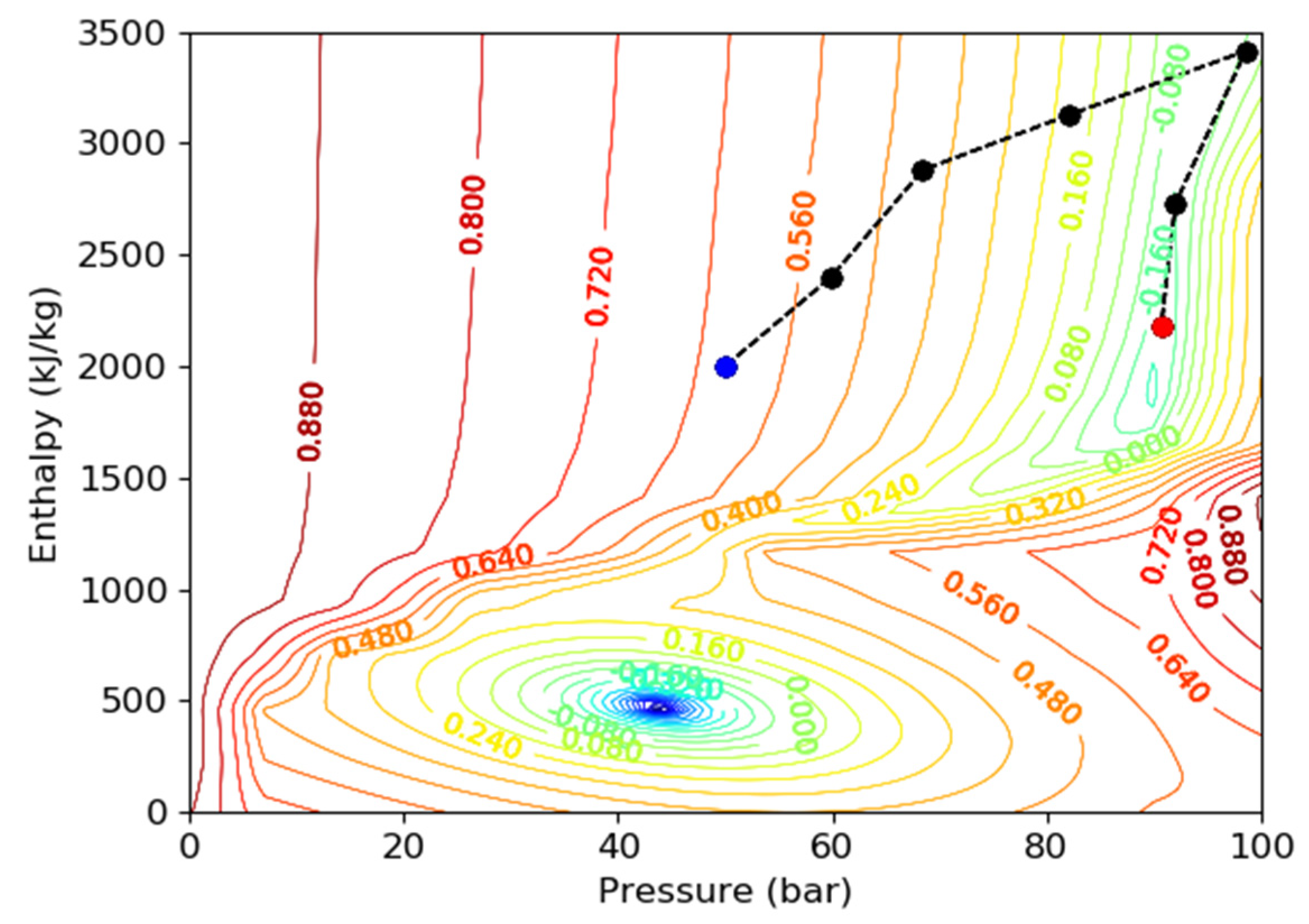
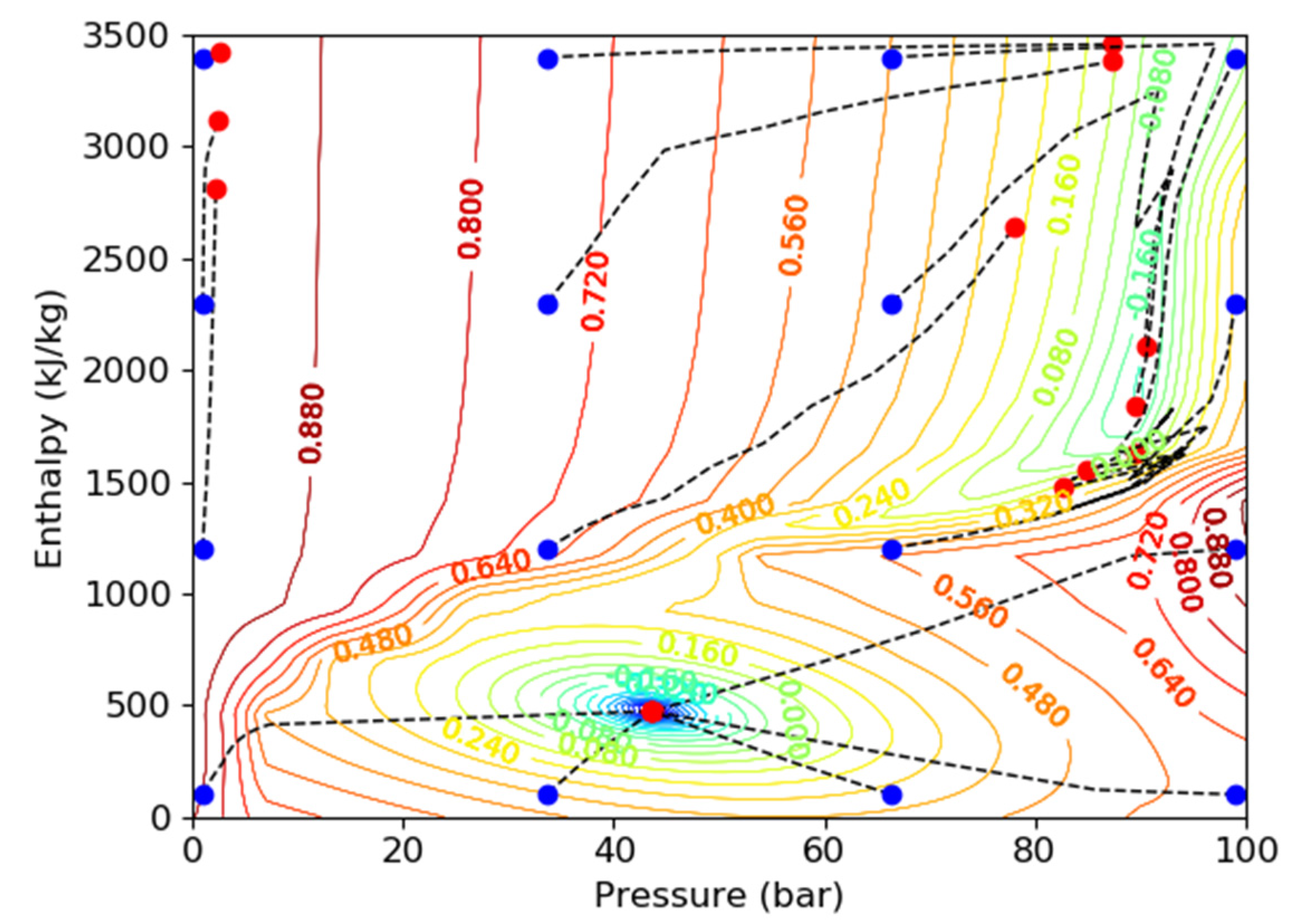
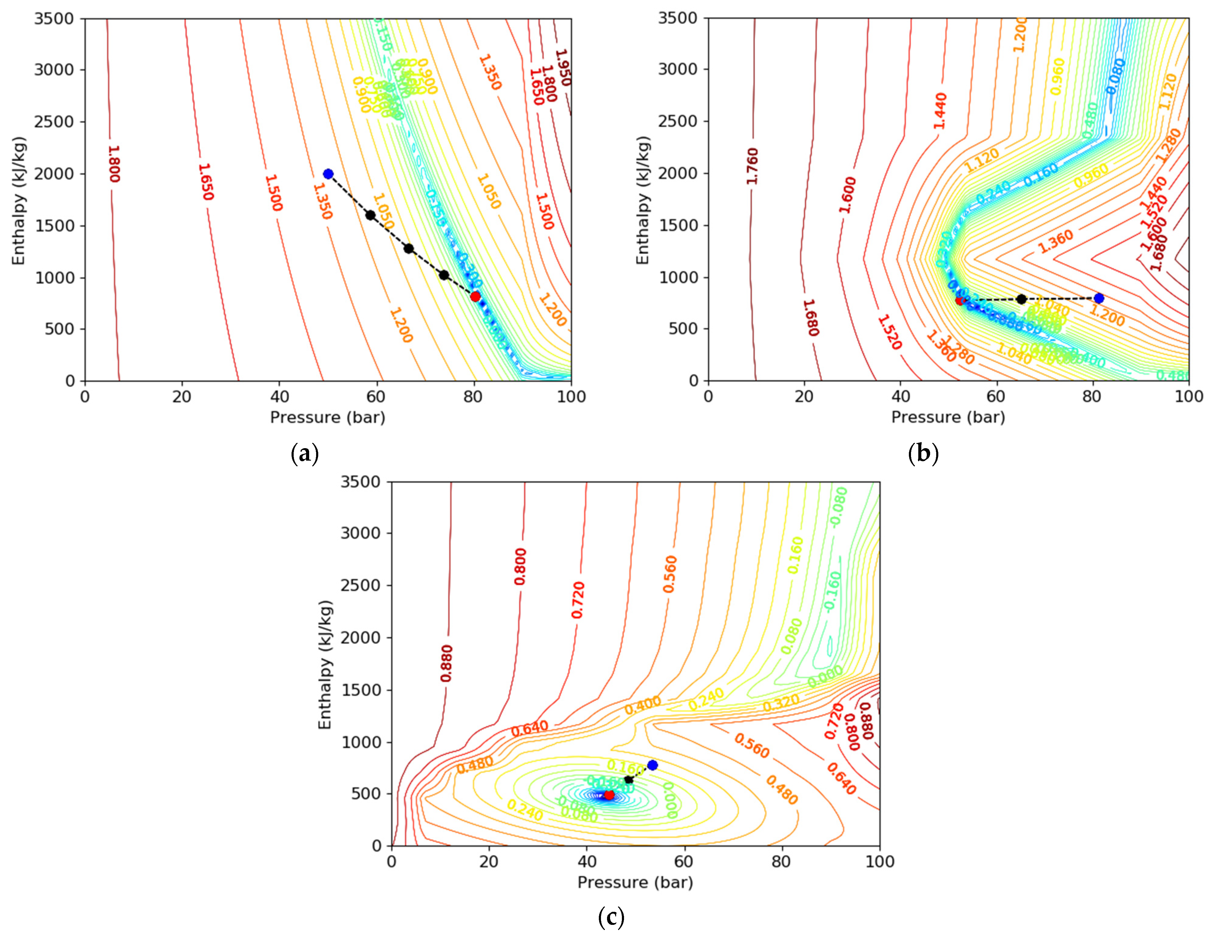
Since mass and energy conservation equations are tightly coupled through the fluid thermodynamics in high-enthalpy geothermal processes, they are usually solved in a fully implicit manner. The ‘negative compressibility’ phenomena can significantly impede the convergence of the nonlinear solver. Because of the large variation in thermodynamic properties between water and steam, the governing equations show high nonlinearity with phase transition. We analyze the problem in a single-cell setup with a cold water injection at fixed pressure. The analysis of the residual map demonstrates that two different minima can be present in the parameter space when simulation is performed with a sufficiently large timestep, which brings challenges for a gradient-based nonlinear solver. A suitable initial guess is essential for the Newton-based nonlinear strategy.
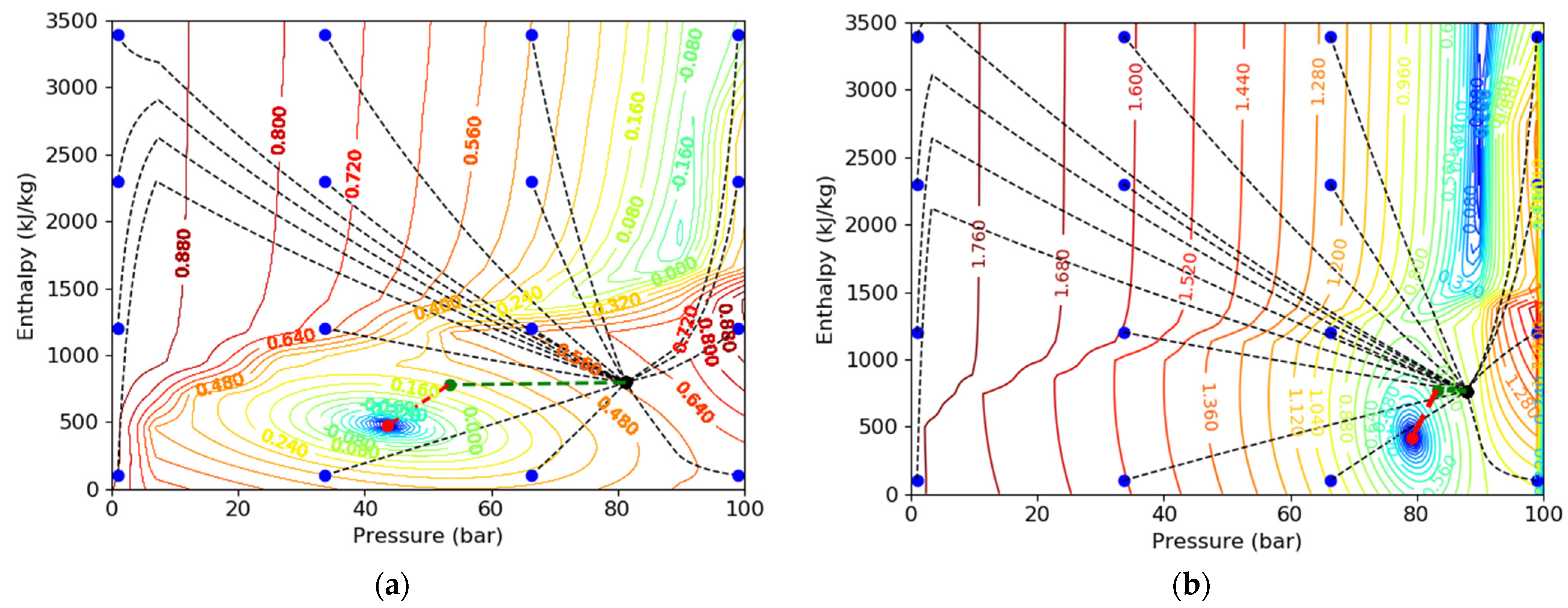
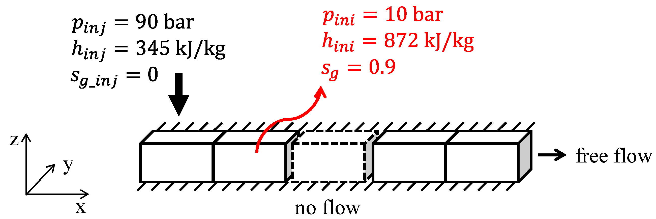
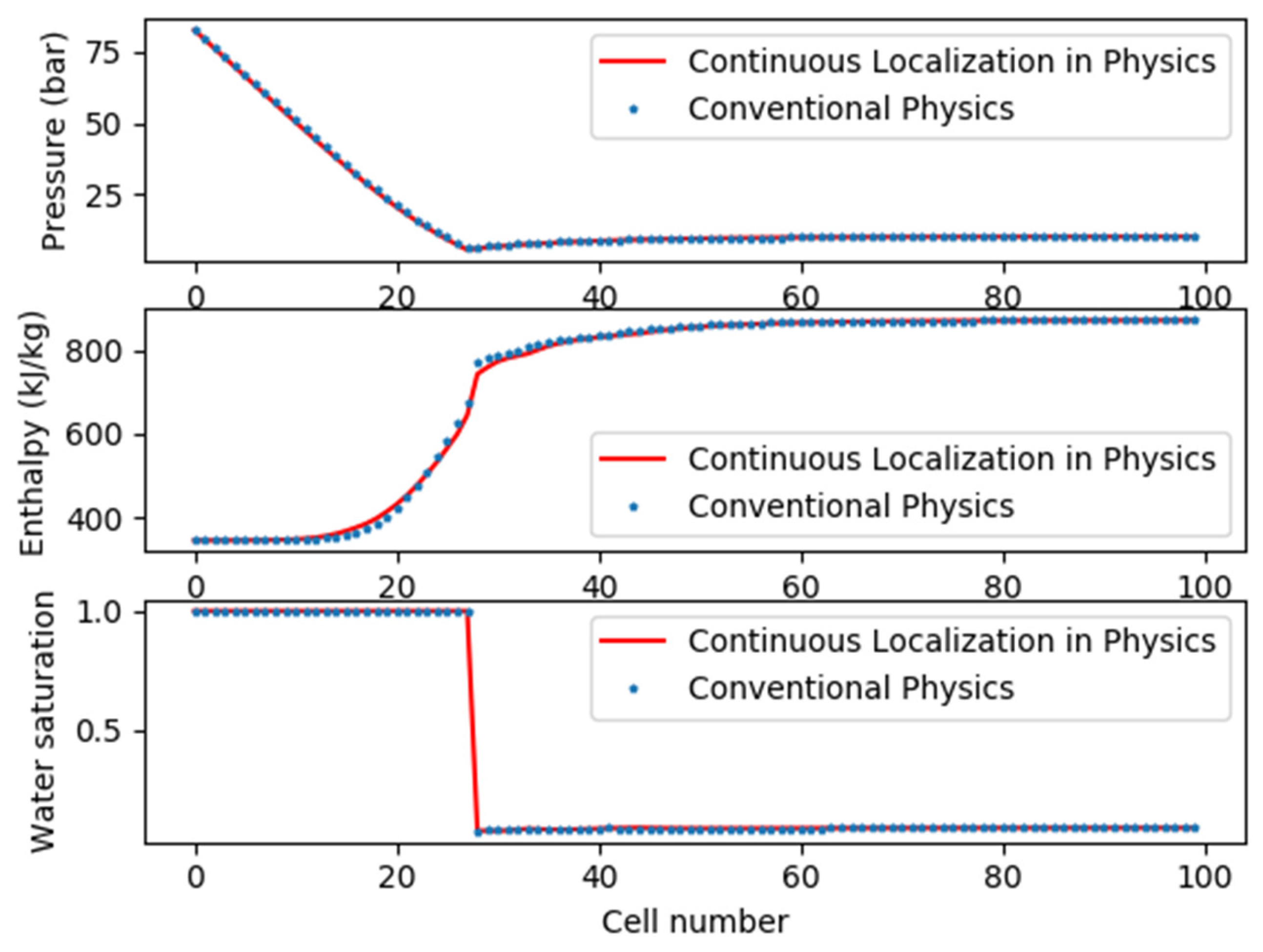
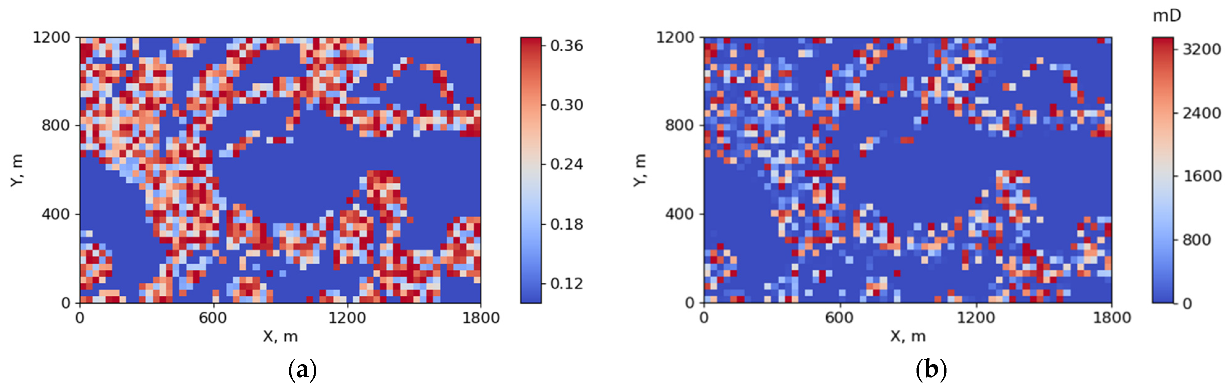
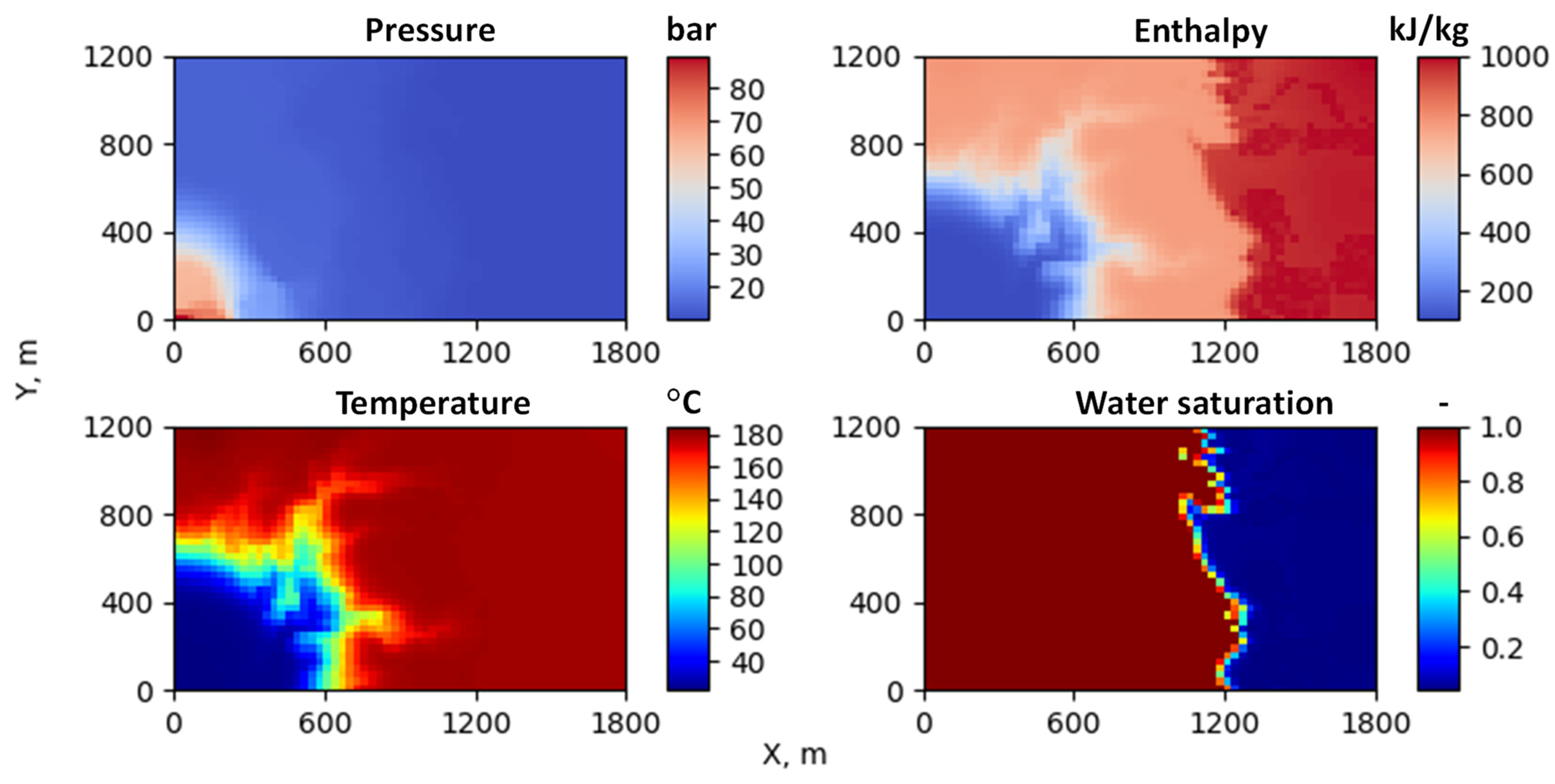
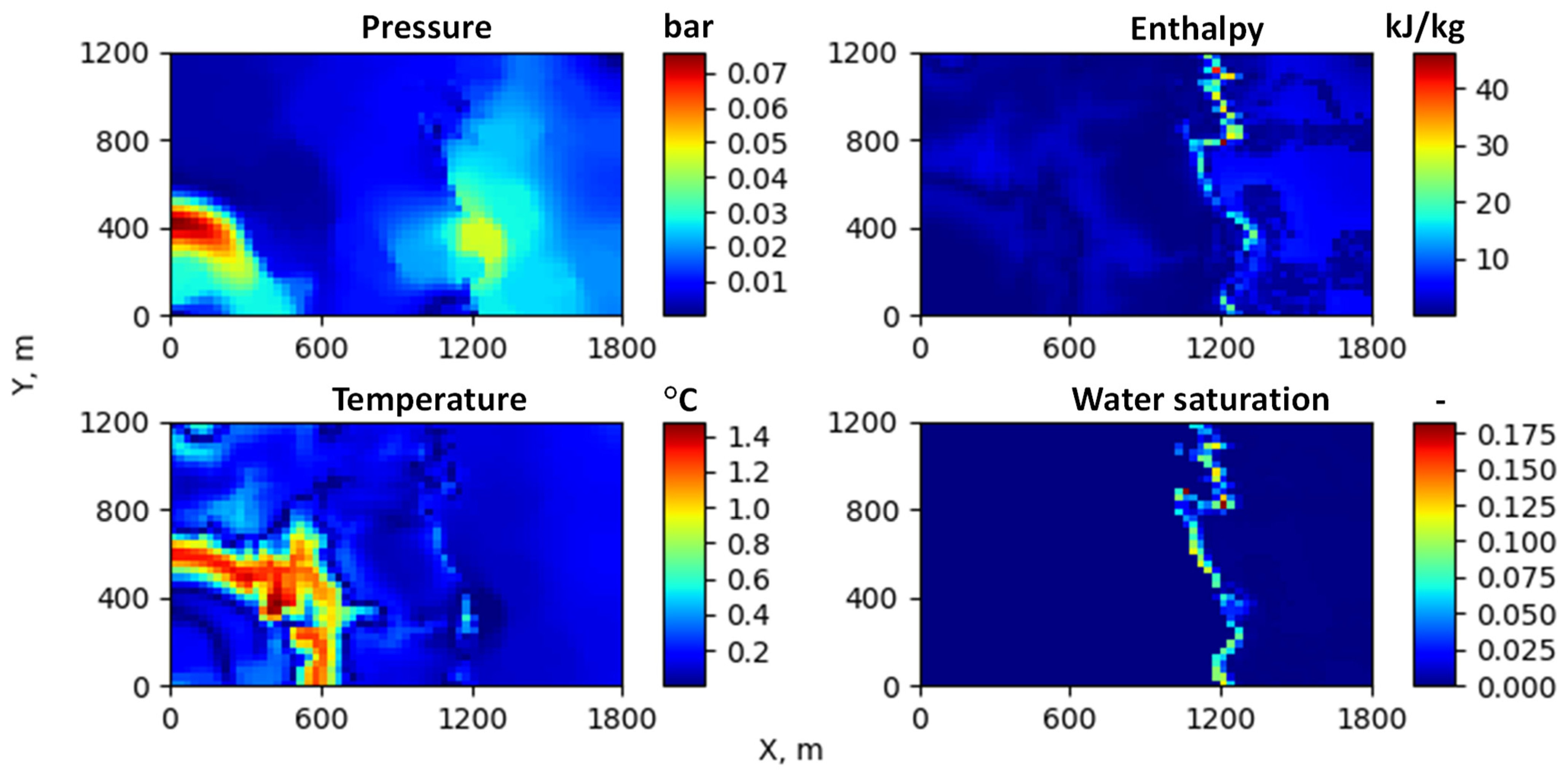
Applying the Operator-Base Linearization approach, we propose the continuous localization in physics method to solve the governing system of equations. With parametrization in physics changing from a coarse to fine resolution, the state-dependent operators and resulting residual changes from an almost linear and monotone behavior to a highly nonlinear and non-monotone shape. In the proposed nonlinear strategy, the solution at a coarser parametrization in physics is taken as an initial guess for the solution at a finer physical resolution. This continuous localization approach makes the nonlinear convergence process more robust in the presence of the ‘negative compressibility’ phenomena. To verify the feasibility of this approach, we prepare synthetic one- and two-dimensional test cases and make a comparison between the conventional and proposed approaches. The results demonstrate that the simulation of high-enthalpy geothermal applications can benefit from continuous localization by running the model at a sufficiently large timestep with a limited number of nonlinear iterations.

Author Contributions

Conceptualization, Y.W. and D.V.; methodology, D.V.; software, Y.W.; validation, Y.W. and D.V.; formal analysis, Y.W.; investigation, Y.W.; resources, D.V.; data curation, Y.W.; writing—original draft preparation, Y.W.; writing—review and editing, D.V.; visualization, Y.W.; supervision, D.V.; project administration, D.V.; funding acquisition, D.V. All authors have read and agreed to the published version of the manuscript.

Funding

This research received no external funding.

Data Availability Statement

The data presented in this study are available on request from the corresponding author.

Acknowledgments

We acknowledge Yang Wong and Mark Khait for their technical help and useful discussions.

Conflicts of Interest

The authors declare no conflict of interest.

References

  1. O’Sullivan, M.; Yeh, A.; Mannington, W. Renewability of geothermal resources. Geothermics 2010, 39, 314–320. [Google Scholar] [CrossRef]
  2. Lund, J.; Boyd, T. Direct utilization of geothermal energy 2015 worldwide review. Geothermics 2016, 60, 66–93. [Google Scholar] [CrossRef]
  3. Barbier, E. Geothermal energy technology and current status: An overview. Renew. Sustain. Energy Rev. 2002, 6, 3–65. [Google Scholar] [CrossRef]
  4. Limberger, J.; Boxem, T.; Pluymaekers, M.; Bruhn, D.; Manzella, A.; Calcagno, P.; Beekman, F.; Cloetingh, S.; van Wees, J.D. Geothermal energy in deep aquifers: A global assessment of the resource base for direct heat utilization. Renew. Sustain. Energy Rev. 2018, 82, 961–975. [Google Scholar] [CrossRef]
  5. Kivanc Ates, H.; Serpen, U. Power plant selection for medium to high enthalpy geothermal resources of Turkey. Energy 2016, 102, 287–301. [Google Scholar] [CrossRef]
  6. Coats, K.H.; George, W.D.; Chu, C.; Marcum, B.E. Three-dimensional simulation of steamflooding. Soc. Pet. Eng. J. 1974, 14, 573–592. [Google Scholar] [CrossRef]
  7. Coats, K.H. Reservoir simulation: A general model formulation and associated physical/numerical sources of instability. In Proceedings of the BAIL I Conference held at Trinity College, Dublin, Ireland, 1 January 1980. [Google Scholar]
  8. Pruess, K.; Oldenburg, C.M.; Moridis, G.J. Tough2 User’s Guide; Lawrence Berkeley National Lab. (LBNL): Berkeley, CA, USA, 1999.
  9. Pruess, K.; Calore, C.; Celati, R.; Wu, Y.S. An analytical solution for heat transfer at a boiling front moving through a porous medium. Int. J. Heat Mass Transf. 1987, 30, 2595–2602. [Google Scholar] [CrossRef]
  10. Falta, R.W.; Pruess, K.; Javandel, I.; Witherspoon, P.A. Numerical modeling of steam injection for the removal of nonaqueous phase liquids from the subsurface: 1. Numerical formulation. Water Resour. Res. 1992, 28, 433–449. [Google Scholar] [CrossRef] [Green Version]
  11. Wang, Y. A stability criterion for the negative compressibility problem in geothermal simulation and discrete modeling of failure in oil shale pyrolysis process. Master’s Thesis, Stanford University, Stanford, CA, USA, 2015. [Google Scholar]
  12. Wong, Z.Y.; Horne, R.; Voskov, D. A geothermal reservoir simulator in AD-GPRS. In Proceedings of the World Geothermal Congress, Melbourne Convention and Exhibition Center (MCEC), Melbourne, Australia, 13–16 September 2018. [Google Scholar]
  13. Wong, Z.Y.; Rin, R.; Tchelepi, H.; Horne, R. Comparison of fully implicit and sequential implicit formulation for geothermal reservoir simulations. In Proceedings of the Workshop on Geothermal Reservoir Engineering, Stanford University, Stanford, CA, USA, 3–15 February 2017. [Google Scholar]
  14. Wagner, W.; Kretzschmar, H.J. International Steam Tables: Properties of Water and Steam Based on the Industrial Formulation IAPWS-IF97; Springer Science & Business Media: Berlin/Heidelberg, Germany, 2019. [Google Scholar]
  15. Collins, D.A.; Nghiem, L.X.; Li, Y.K.; Grabenstetter, J.E. An efficient approach to adaptive-implicit compositional simulation with an equation of state. SPE Reserv. Eng. 1992, 7, 259–264. [Google Scholar] [CrossRef]
  16. Voskov, D. Operator-based linearization approach for modeling of multiphase multi-component flow in porous media. J. Comput. Phys. 2017, 337, 275–288. [Google Scholar] [CrossRef]
  17. Wang, Y.; Voskov, D.; Khait, M.; Saeid, S.; Bruhn, D. Influential factors on the development of a low-enthalpy geothermal reservoir: A sensitivity study of a realistic field. Renew. Energy 2021, 179, 641–651. [Google Scholar] [CrossRef]
  18. Delft Advanced Research Terra Simulator. Available online: https://darts.citg.tudelft.nl (accessed on 1 October 2022).
  19. Wang, Y.; Voskov, D.; Khait, M.; Bruhn, B. An efficient numerical simulator for geothermal simulation: A benchmark study. Appl. Energy 2020, 264, 114693. [Google Scholar] [CrossRef]
  20. Faust, C.R.; Mercer, J.W. Summary of our research in geothermal reservoir simulation. In Proceedings of the Workshop on Geothermal Reservoir Engineering, Stanford University, Stanford, CA, USA, 15–17 December 1975. [Google Scholar]
  21. Khait, M.; Voskov, D. Operator-based linearization for efficient modeling of geothermal processes. Geothermics 2018, 74, 7–18. [Google Scholar] [CrossRef]
  22. Wong, Z.Y.; Horne, R.; Tchelepi, H. Sequential implicit nonlinear solver for geothermal simulation. J. Comput. Phys. 2018, 368, 236–253. [Google Scholar] [CrossRef]
Figure 1. Newton path (dash line) starts from the initial condition; the contours (in l 2 −norm) show the residuals; the blue dot represents the initial condition of the cell; the black dots are the Newton updates; the red dot shows the solution for a current timestep.
Mathematics 10 04328 g001
Figure 2. Newton paths (dash line) start from various points in pressure−enthalpy space; the contours (in l 2 −norm) show the residuals, blue dots represent the initial guess, red dots show the solution for a current timestep.
Mathematics 10 04328 g002
Figure 3. Operators in mass and energy conservation equations for the single-cell problem. (a) Mass accumulation operator, (b) energy accumulation operator, (c) mass flux operator, (d) energy flux operator. The color changing from deep blue to red represents the magnitude of the operator values varying from low to high.
Mathematics 10 04328 g003aMathematics 10 04328 g003b
Figure 4. Newton path and residual contours (in l 2 −norm) with continuation parameterization in physics: (a) Newton path for a coarse resolution; (b) Newton path for an intermediate resolution; (c) Newton path for a fine (reference) resolution; the blue dot represents the initial guess, the black dot is the Newton update, the red dot shows the solution.
Mathematics 10 04328 g004
Figure 5. The flowchart to illustrate the idea of the proposed continuous localization in physics.
Mathematics 10 04328 g005
Figure 6. Newton path (dashed line) starting from various points in pressure-enthalpy space with (a) moderate and (b) large timestep; the blue dots represent the initial guess, the black dot is the solution of the coarsest resolution, the green dot is the intermediate solution and the red dot is the true solution; dashed lines in black, green and red represent the Newton path in the coarse, intermediate and fine (reference) physical resolutions, respectively; residual contours (in l 2 −norm) are plotted for the reference physics.
Mathematics 10 04328 g006
Figure 7. Schematics of 1D test case. p i n i and h i n i refer to the initial pressure and enthalpy of the model, respectively, and s g refers to the initial steam saturation of the model. p i n j and h i n j are the injection pressure and enthalpy, and s g _ i n j is the injection steam saturation.
Mathematics 10 04328 g007
Figure 8. Simulation results with continuous localization in physics with a large timestep (red line) and a conventional Newton-based approach with the reduced timestep (blue dots).
Mathematics 10 04328 g008
Figure 9. The porosity and permeability distribution of the two-dimensional setup. (a) Porosity field; (b) permeability field.
Mathematics 10 04328 g009
Figure 10. The pressure, enthalpy, temperature and water saturation maps of the model after one-year simulation with the proposed continuous localization of the Newton method.
Mathematics 10 04328 g010
Figure 11. The difference in the pressure, enthalpy, temperature and water saturation solutions between the conventional method and the proposed continuous localization of the Newton method with similar running timesteps.
Mathematics 10 04328 g011
Table 1. The statistics of the 1D model.
ParametersConventional MethodContinuous Localization in Physics Method
Resolution of parameterization in (p, h) space(128, 128)(128, 4) » (128, 8) »
(128, 32) » (128, 128)
Total Newton iteration3325683
Wasted Newton iteration76080
CPU time, second14.94.2
Table 2. The initial and injection conditions of the model.
ParametersUnitValues
Initial pressurebar10
Initial enthalpykJ/kg1000
Initial water saturation-0.04
Injection pressurebar90
Injection enthalpykJ/kg100
Injection water saturation-1.0
Table 3. Comparison of the statistics of the two methods.
ParametersConventional MethodContinuous Localization in Physics Method
Resolution of parameterization in (p, h) space(128, 128)(128, 4) » (128, 8) »
(128, 32) » (128, 128)
Total Newton iteration2374873
Wasted Newton iteration1140280
CPU time, second9637
Publisher’s Note: MDPI stays neutral with regard to jurisdictional claims in published maps and institutional affiliations.

