A Novel Coupled Meshless Model for Simulation of Acoustic Wave Propagation in Infinite Domain Containing Multiple Heterogeneous Media

Abstract

This study presents a novel coupled meshless model for simulating acoustic wave propagation in heterogeneous media, based on the singular boundary method (SBM) and Kansa’s method (KS). In the proposed approach, the SBM was used to model the homogeneous part of the propagation domain, while KS was employed to model a heterogeneity. The interface compatibility conditions associated with velocities and pressures were imposed to couple the two methods. The proposed SBM–KS coupled approach combines the respective advantages of the SBM and KS. The SBM is especially suitable for solving external sound field problems, while KS is attractive for nonlinear problems in bounded non-homogeneous media. Moreover, the new methodology completely avoids grid generation and numerical integration compared with the finite element method and boundary element method. Numerical experiments verified the accuracy and effectiveness of the proposed scheme.

1. Introduction

The propagation of sound waves in fluids and solids is an important issue in science and engineering. In the past few decades, the boundary element method (BEM) has become established as an effective tool for sound propagation analysis, especially for the infinite and semi-infinite domains [1,2,3,4], due to the used fundamental solution automatically satisfying the far-field radiation condition. Compared with other well-established mesh-based methods, such as the finite element method (FEM) [5,6,7,8] and the finite difference method (FDM) [9,10], the BEM can solve acoustic problems merely through boundary discretization. However, it involves a sophisticated mathematical formulation and a tedious estimation of singular and hyper-singular integrals [11,12]. Furthermore, these methods require the use of domain truncation techniques for infinite domain problems for the numerical solution of problems on unbounded domains.

In recent years, various meshless/meshfree methods [13,14,15,16,17,18,19] have been proposed to reduce or even eliminate the tasks of mesh generation and singular integration. Among these approaches, the singular boundary method (SBM) [20,21,22,23] is a boundary-only discretization meshless technique, which does not require mesh generation and numerical integration. This method is very simple and accurate for the analysis of sound fields in unbounded domains, since it also employs the fundamental solution satisfying the governing equation and the far-field radiation condition [24,25]. Another common meshless scheme is Kansa’s method (KS) [26,27,28,29], which is based on the radial basis function (RBF). This method does not require the fundamental solution, and is suitable for solving arbitrary partial differential equations in bounded domains [30,31,32,33].

As can be inferred from above, the SBM and KS have their respective advantages in addressing unbounded homogeneous media and bounded non-homogeneous media. In order to avoid complex computational processes such as mesh generation and singular integral computation using traditional methods such as the FEM and the BEM, this research made a first attempt to couple these two methods (named SBM–KS) for simulating acoustic wave propagation in heterogeneous media. The SBM is adopted to model the homogeneous part of the propagation domain, while KS is employed to model a heterogeneity. A direct coupling strategy between the SBM and KS is presented based on the continuity conditions of velocities and pressures on the interface. The coupling method shows unique advantages in solving such problems compared to existing methods, such as simplicity, accuracy, and being free of mesh and integration.

The organization of this manuscript is as follows: Section 2 briefly describes acoustic wave propagation problems of heterogeneous media. Section 3 introduces the SBM for an unbounded acoustic medium, KS for a heterogeneous acoustic medium, and the coupling strategy of these two methods. In Section 4, two classical numerical examples are provided to verify the accuracy and effectiveness of the proposed methodology. Finally, Section 5 provides some conclusions and remarks.

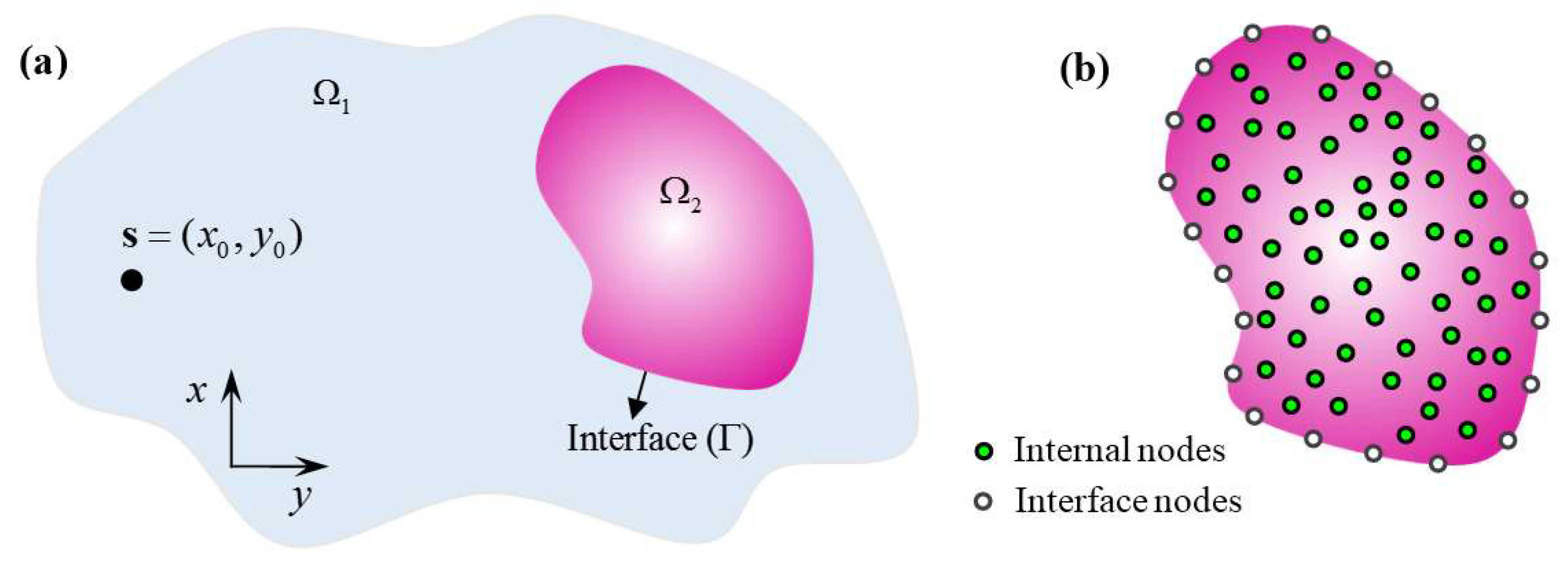
2. Problem Statement

Consider an unbounded homogeneous medium ${\Omega }_1$, containing a subdomain ${\Omega }_2$ in which the sound velocity is variable (see Figure 1a), and the sound field is excited by a harmonic pressure source at position $s=(x_0,y_0)$. In this regard, the sound waves travel at a constant speed $v_1(x)=v_1$ in ${\Omega }_1$ and a variable speed $v_1(x)$ in ${\Omega }_2$ at $x=(x,y)$. Then, the acoustic pressure fields $p_1(x)$ and $p_2(x)$ within homogeneous and heterogeneous media can be described by the following Helmholtz equations:

$${\nabla }^2{p}_1(x)+{\left[\frac{\omega }{v_1}\right]}^2{p}_1(x)=0, x\in {\Omega }_1,$$

(1)

$${\nabla }^2{p}_2(x)+{\left[\frac{\omega }{v_2(x)}\right]}^2{p}_2(x)=0, x\in {\Omega }_2,$$

(2)

where ${\nabla }^2$ is the Laplace operator, and $\omega$ is the angular frequency.

Notice that the governing equations are the PDEs with constant and variable coefficients in domains ${\Omega }_1$ and ${\Omega }_2$, respectively. The conventional boundary-type methods, such as the BEM, the SBM, and the fundamental solution method, cannot be directly applied to solve variable-coefficient PDEs. Meanwhile, domain-type methods, such as the FEM, the meshless local Petrov–Galerkin (MLPG) method and Kansa’s method, require the truncation of boundaries and the division of grids, which is extremely troublesome when dealing with problems in infinite homogeneous media. It should be noticed that the fundamental solution employed in the SBM automatically satisfies the Sommerfeld radiation condition at infinity:

$$\underset{r\to \infty }{\lim }{r}^{\frac{1}{2}(d-1)}(\frac{\partial p(\mathit{x})}{\partial r}-\mathrm{i}kp(\mathit{x}))=0$$

(3)

where d is the spatial dimension, $\mathrm{i}=\sqrt{-1}$ is the imaginary unit, k is the wave number, and r is the distance between point x and the sound field’s center.

In the present study, the above-mentioned problem was solved by coupling the SBM and KS to overcome the limitations posed separately by each method. The SBM was employed to model the unbounded acoustic medium, while KS was used to model the heterogeneous medium. The coupling between the two approaches was accomplished by utilizing continuity conditions of pressures and velocities on the boundary of the heterogeneous medium. Figure 1b illustrates the schematic diagram of the nodal distribution for the coupled meshless model. The two methods used the same nodes on the interface.

3. Methodology

3.1. SBM for Unbounded Acoustic Medium

Assuming the total number of nodes on the interface is M, the sound pressure at point $\mathit{x}\in {\Omega }_1\cup \Gamma$ can be calculated by the following SBM formula:

$${\widehat{p}}_1(\mathit{x})={\displaystyle \sum _{j=1}^M{\alpha }_{j}G(\mathit{x},{\mathit{x}}_j)}+p_{inc}({\mathit{x}}_i,s), {\mathit{x}}_j\in \Gamma$$

(4)

where ${\alpha }_j$ is the unknown coefficient, ${\mathit{x}}_j$ is the boundary node shown in Figure 1b, $p_{inc}({\mathit{x}}_i,s)=H_0^{(2)}(\frac{\omega }{v_1}{\Vert {\mathit{x}}_i-s\Vert }_2)$ represents the incident pressure field generated by a harmonic pressure source at position $s=(x_0,y_0)$ in the domain ${\Omega }_1$, and $G(\mathit{x},{\mathit{x}}_j)$ is the fundamental solution of the Helmholtz equation, which is given by the following:

$$G(\mathit{x},{\mathit{x}}_j)=-\frac{\mathrm{i}}{4}{H}_0^{(2)}\left(\frac{\omega }{v_1}{\Vert \mathit{x}-{\mathit{x}}_j\Vert }_2\right)$$

(5)

where $H_0^{(2)}$ is the zeroth-order Hankel function of the second kind.

To solve the unknown coefficients ${\left\{{\alpha }_j\right\}}_{j=1}^M$, let $\mathit{x}$ in Equation (4) be the boundary node ${\mathit{x}}_j$; we have the following equations for the Dirichlet boundary condition:

$${\widehat{p}}_1({\mathit{x}}_i)={\displaystyle \sum _{\begin{array}{l}j=1\\ i\ne j\end{array}}^M{\alpha }_{j}G({\mathit{x}}_i,{\mathit{x}}_j)}+{\alpha }_i{p}_{ii}+p_{inc}({\mathit{x}}_i,s), i=1,2,\dots ,M,$$

(6)

and for the Neumann boundary condition, we have the following:

$$\frac{\partial {\widehat{p}}_1({\mathit{x}}_i)}{\partial n_{x_i}}={\displaystyle \sum _{\begin{array}{l}j=1\\ i\ne j\end{array}}^M{\alpha }_j\frac{\partial G({\mathit{x}}_i,{\mathit{x}}_j)}{\partial n_{x_i}}}+{\alpha }_i{q}_{ii}+\frac{\partial p_{inc}({\mathit{x}}_i,s)}{\partial n_{x_i}}, i=1,2,\dots ,M,$$

(7)

where ${\mathit{x}}_i$ and ${\mathit{x}}_j$ denote the ith and jth boundary nodes, $p_{ii}$ and $q_{ii}$ are the origin intensity factors when the source point and the field point coincide (i.e., $i=j$), which can be computed using the following formulas in references [34,35]:

$$u_{ii}=\frac{\mathrm{i}}{4}-\frac{1}{2\mathsf{\pi }}\left(\ln \left(\frac{L_i}{2\mathsf{\pi }}\right)+\ln \left(\frac{k}{2}\right)+\gamma \right),$$

(8)

$$q_{ii}=\frac{1}{L_i}-{\displaystyle \sum _{\begin{array}{l}j=1\\ j\ne i\end{array}}^N{\zeta }_{ji}\frac{\partial G_0({\mathit{x}}_i,{\mathit{s}}_j)}{\partial {\mathit{n}}_s}},$$

(9)

where $L_i$ is the influence range of the boundary point ${\mathit{x}}_i$ (see Figure 2), $\gamma$ is the Euler constant, $G_0({\mathit{x}}_i,{\mathit{x}}_j)$ the fundamental solution of the Laplace equation, as follows:

$$G_0({\mathit{x}}_i,{\mathit{x}}_j)=-\frac{1}{2\mathsf{\pi }}\ln {\Vert {\mathit{x}}_i-{\mathit{x}}_j\Vert }_2.$$

(10)

For the convenience of coupling calculations, Equations (6) and (7) can be written in the following matrix forms:

$${\widehat{\mathbf{p}}}_1=\mathbf{G}\mathsf{\alpha }+{\mathbf{p}}_{\mathrm{in}},$$

(11)

$${\widehat{\mathbf{q}}}_1=\mathbf{H}\mathsf{\alpha }+{\mathbf{q}}_{\mathrm{in}}.$$

(12)

3.2. Kansa’s Method for Inhomogeneous Acoustic Medium

For the closed domain ${\Omega }_2$ with the boundary $\Gamma$, we chose a set of N collocation points, including $Ni$ internal points and M boundary points, as shown in Figure 1b. According to the basic idea of KS, the sound pressure in subdomain ${\Omega }_2$ can be approximated using a linear combination of RBFs, as follows:

$${\widehat{p}}_2(x)={\displaystyle \sum _{k=1}^N{\beta }_k}{\phi }_k(x),$$

(13)

where ${\beta }_k$ is the unknown coefficient to be determined, and ${\phi }_k(x)$ is the multiquadric (MQ) RBF function, which is defined as the following:

$${\phi }_k(x)=\sqrt{r_k^2+c^2},$$

(14)

where $r_k={\Vert x-x_k\Vert }_2$ is the distance between nodes $x$ and $x_k$, and c is the shape parameter, which is fixed at 0.5 in this study. The MQ-RBF is a highly sought-after function due to its numerous advantages for various applications. Its main advantages include the following: (1) Smoothness: it is a smooth function with continuous derivatives of all orders, which is a crucial requirement for many applications. (2) Accuracy: it offers exceptional approximation accuracy for a wide range of functions and can converge faster than other RBFs for some problems, making it an excellent choice for large-scale applications. (3) Scalability: it is computationally efficient, making it a perfect fit for large-scale problems. It has a low computational cost for interpolation and can be easily parallelized. (4) Robustness: it is less sensitive to data outliers than other RBFs, making it a robust choice for applications where data may contain noise or outliers. (5) Universality: it is a universal approximator, meaning it can approximate any continuous function to any desired accuracy, given sufficient data points.

Substituting Equation (13) into Equation (1) for internal nodes, one obtains the following:

$${\nabla }^2{\displaystyle \sum _{k=1}^N{\beta }_k}{\phi }_k(x_i)+{\left[\frac{\omega }{v_2(x_i)}\right]}^2{\displaystyle \sum _{k=1}^N{\beta }_k}{\phi }_k(x_i)=0, {\mathit{x}}_i\in {\Omega }_2$$

(15)

In addition, the sound pressure and its normal derivative at the boundary nodes satisfy the following equations:

$${\widehat{p}}_2(x_i)={\displaystyle \sum _{k=1}^N{\beta }_k}{\phi }_k(x_i), {\mathit{x}}_i\in \Gamma ,$$

(16)

$$\frac{\partial {\widehat{p}}_2(x_i)}{\partial n_{x_i}}={\displaystyle \sum _{k=1}^N{\beta }_k}\frac{\partial {\phi }_k(x_i)}{\partial n_{x_i}}, {\mathit{x}}_i\in \Gamma .$$

(17)

Equations (15)–(17) can be rewritten in the following matrix forms:

$$\mathbf{R}\mathsf{\beta }=0,$$

(18)

$${\widehat{p}}_2=\mathbf{B}\mathsf{\beta },$$

(19)

$${\widehat{q}}_2=\mathbf{F}\mathsf{\beta }.$$

(20)

3.3. Coupled Model Dymamic System

This study proposed a direct coupling strategy between the two methods, under the condition that the nodes used in the SBM model matched the boundary nodes used in KS. Note the following:

$$\frac{\partial p(x)}{\partial n_x}=-\mathrm{i}\rho \omega v(x),$$

(21)

where the coupled system can be established by employing the continuity of pressure and velocity on the interface between the two media, which can be expressed as follows:

$$p_1(x)=p_2(x) \mathrm{or} {\mathbf{p}}_1={\mathbf{p}}_2, x\in \Gamma ,$$

(22)

$$\frac{\partial p_1(x)}{\partial n_x}=-\frac{\partial p_2(x)}{\partial n_{x_{}}} \mathrm{or} {\mathbf{q}}_1={\mathbf{q}}_2, x\in \Gamma .$$

(23)

Considering all the nodes within the domain ${\Omega }_2$, and using the above continuity conditions, Equations (11), (12), and (18)–(20) can be combined to form a total linear system, namely, the following:

$$\left[\begin{array}{cc}\mathbf{G}& -\mathbf{B}\\ \mathbf{H}& \mathbf{F}\\ \mathbf{0}& \mathbf{R}\end{array}\right]\left[\begin{array}{l}\mathsf{\alpha }\hfill \\ \mathsf{\beta }\hfill \end{array}\right]=\left[\begin{array}{l}-{\mathbf{p}}_{\mathrm{in}}\hfill \\ -{\mathbf{q}}_{\mathrm{in}}\hfill \\ \mathbf{0}\hfill \end{array}\right]$$

(24)

After solving Equation (24), unknown coefficient vectors $\mathsf{\alpha }$ and $\mathsf{\beta }$ can be determined. Then, the sound pressures at any position in medium ${\Omega }_1$ and ${\Omega }_2$ can be easily obtained by employing Equations (4) and (13).

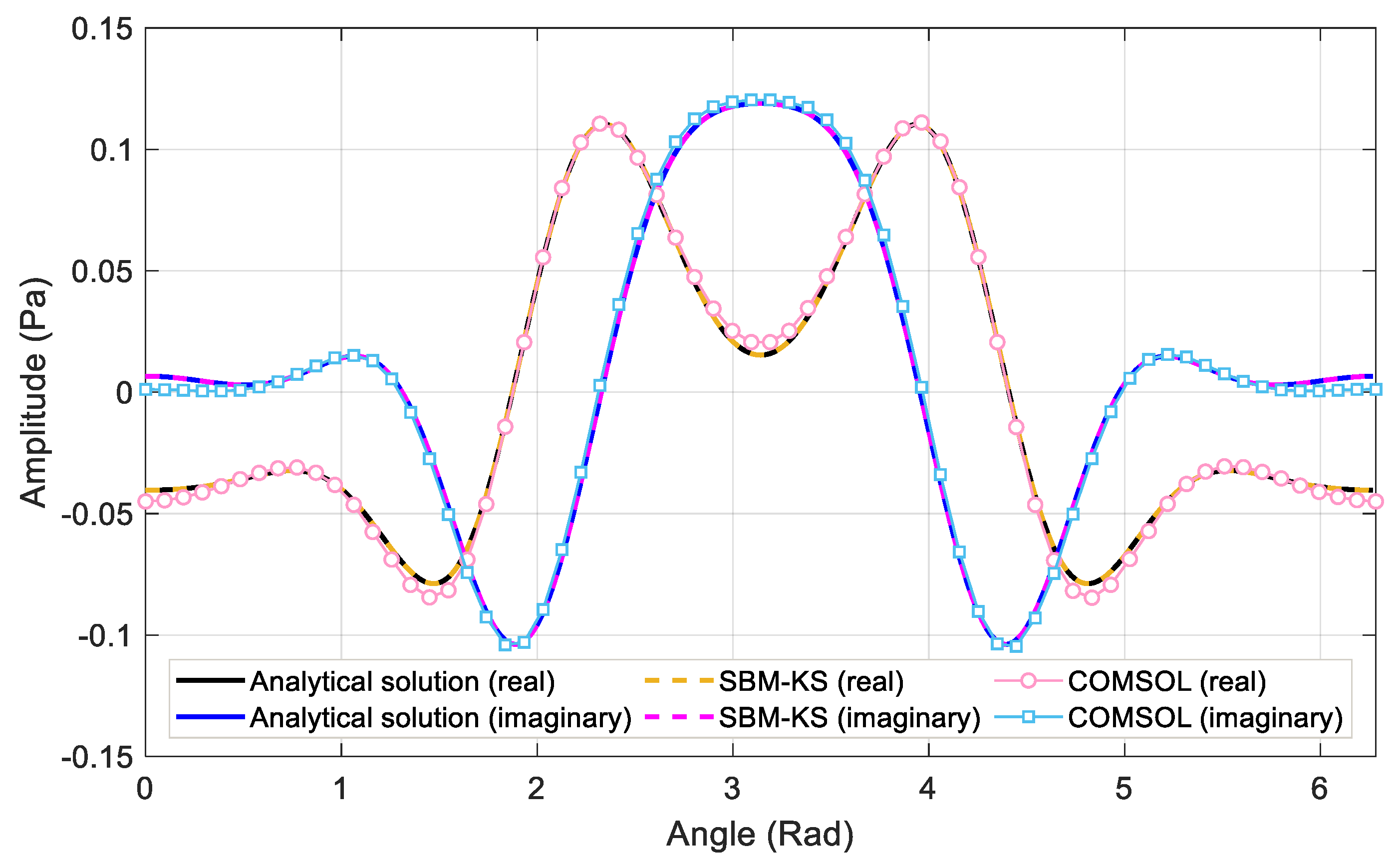
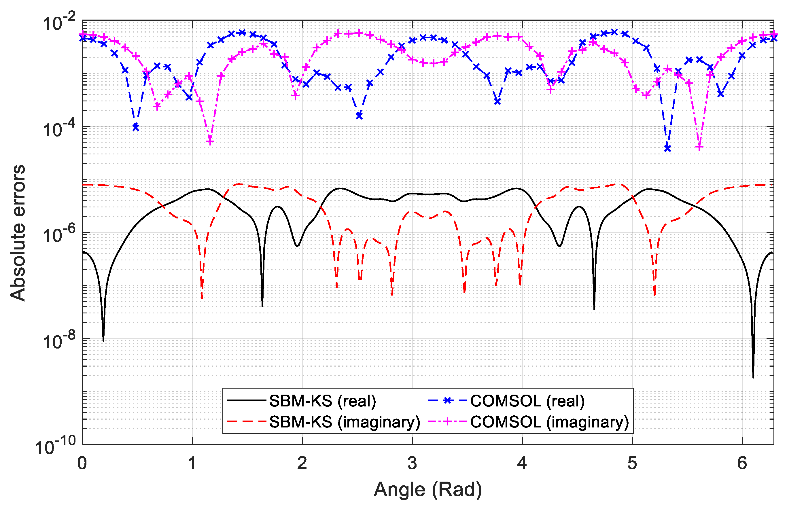
4. Numerical Results and Discussion

In this section, we examine the proposed SBM–KS by three numerical examples, including single and multiple heterogeneous inclusion materials. To assess the numerical errors, the following absolute error was employed:

$$Absolute error=\left|p_{num}(x)-p_{ana}(x)\right|,$$

(25)

where $p_{num}(x)$ and $p_{ana}(x)$ represent the numerical and analytical solutions at point x, respectively. Note that p can be a real part or an imaginary part of the sound pressure.

Example 1.

We consider an infinite homogenous fluid medium with a circular inclusion of radius 1.0 m [36]. The sound velocities are 1500 m/s and 2500 m/s in the infinite fluid medium and the circular inclusion, respectively. Both media have a same density of 1000 kg/m³. The pressure source is placed at ($x_0=-5 \mathrm{m}, y_0=0 \mathrm{m}$).

To numerically solve this problem, the SBM–KS chose 100 interface nodes and 688 internal nodes. Figure 3 shows the comparison of the analytical solution [37], and numerical results obtained by the proposed SBM–KS and COMSOL software under a frequency of 1000 Hz. Absolute errors of these two methods are also provided in Figure 4. In the simulation, the finite element method with 7780 elements used the perfectly matched layer. We can see from Figure 3 that the numerical results obtained from the SBM–KS and the COMSOL FEM are in good agreement with the analytical solutions. It can also be clearly observed that the curve of our method completely coincides with the curve of the analytical solution, while the FEM has certain errors. Moreover, it can be noted that the calculation accuracy of the proposed method is at least two orders higher than that of the FEM. In this example, the condition number of the proposed approach is 1.426 × 10¹¹. The SBM has a small condition number, but KS has a large condition number [38], which leads to a large value of the condition number for the final coefficient matrix. However, the method can still obtain accurate numerical results.

Example 2.

This example considers a non-homogeneous circular region of radius 1 m centered at point (0, 0), which is embedded in an unbounded fluid medium. The pressure source with a frequency of 1000 Hz is placed at ($x_0=-2.5 \mathrm{m}, y_0=0 \mathrm{m}$). Both media have a same density of 1000 kg/m³. The outer fluid medium allows sound waves to travel at 1500 m/s, while the non-homogeneous medium allows sound waves to travel at the following:

$$v_2(x,y)=1500+150\left[1+\sin \left(\pi \sqrt{x^2+y^2}+\frac{\pi }{2}\right)\right],$$

(26)

which is illustrated in Figure 5.

In practical problems, the node distribution may be scattered and uneven. As a meshless technique, the proposed SBM–KS can address the non-uniform node distribution in a leisurely manner. In order to test the effect of node distribution on the calculation accuracy, distributions of regular and irregular nodes were investigated in the calculation, as shown in Figure 6. It includes 100 interface nodes and 688 internal nodes.

Figure 7 displays the profiles of the analytical response in the domain $[-2,2]\times [-2,2]$, and Figure 8 and Figure 9 depict the absolute errors of the proposed method under regular and irregular nodes, respectively. It was noted that the numerical solutions are in good agreement with the analytical one for the regular and irregular distributions of nodes, and the numerical errors are small. In this example, the condition number of the proposed approach is 4.665 × 10¹¹.

Example 3.

The last example considers a complex sound propagation problem in a heterogeneous medium, shown in Figure 10. The domain ${\Omega }_1$ is an infinite domain, in which the speed of sound is $v_1=1500 \mathrm{m}/\mathrm{s}$ and the density is ${\rho }_1=1000 \mathrm{kg}/{\mathrm{m}}^3$. The pressure source is placed at ($x_0=-5 \mathrm{m}, y_0=0 \mathrm{m}$). The bounded domains ${\Omega }_2$, ${\Omega }_3$, and ${\Omega }_4$ are all heterogeneous media, and their boundaries can be expressed as the following parameter forms:

$${\Gamma }_2=\left\{\left(x=r_2(\theta )\cos \theta ,y=2+r_2(\theta )\sin \theta \right)|r_2(\theta )=\sqrt[3]{\cos \left(3\theta \right)+\sqrt{2-{\sin }^2(3\theta )}}, 0\le \theta \le 2\pi \right\},$$

(27)

$${\Gamma }_3=\left\{\left(x=r_3(\theta )\cos \theta ,y=-2+r_3(\theta )\sin \theta \right)|r_3(\theta )=e^{\sin \theta }{\sin }^2\theta +e^{\cos \theta }{\cos }^2\theta , 0\le \theta \le 2\pi \right\},$$

(28)

$${\Gamma }_3=\left\{\left(x=4+r_4(\theta )\cos \theta ,y=r_4(\theta )\sin \theta \right)|r_4(\theta )=1, 0\le \theta \le 2\pi \right\}.$$

(29)

In the present study, we assumed that the density of the three heterogeneous media is the same as that of the infinite medium, while these three media allow sound waves to travel at the following velocities:

$$v_2(x,y)=1500+200\left[1+\sin \left(\pi \sqrt{x^2+{(y-2)}^2}/r_2(\overline{\theta })+\frac{\pi }{2}\right)\right], (x,y)\in {\Omega }_2,$$

(30)

$$v_3(x,y)=1500+100\left[1+\sin \left(\pi \sqrt{x^2+{(y+2)}^2}/r_3(\overline{\theta })+\frac{\pi }{2}\right)\right], (x,y)\in {\Omega }_3,$$

(31)

$$v_4(x,y)=1500+150\left[1+\sin \left(\pi \sqrt{{(x-4)}^2+y^2}/r_4(\overline{\theta })+\frac{\pi }{2}\right)\right], (x,y)\in {\Omega }_4,$$

(32)

where $\overline{\theta }$ denotes the azimuth angle of the point (x, y), functions $r_2$, $r_3$, and $r_4$ have are given in Equations (27)–(29). The velocity variations in the domain $[-8,8]\times [-6,6]$ are shown in Figure 11.

In this example, the proposed method was used to solve the problem of sound propagation in an infinite domain with three heterogeneous media. In the calculation, the SBM was employed to simulate the external sound field ${\Omega }_1$, while KS was used to approximate the sound field in heterogeneous media ${\Omega }_2$, ${\Omega }_3$, and ${\Omega }_4$. The two methods were coupled by employing the continuity conditions of pressure and velocity on the interfaces ${\Gamma }_2$, ${\Gamma }_3$, and ${\Gamma }_4$.

In order to obtain accurate and reliable numerical results, a total of 6422 nodes were used in the study. On each interface, 400 nodes were evenly arranged according to the angle. In domains ${\Omega }_2$, ${\Omega }_3$, and ${\Omega }_4$, 1360, 2616, and 1246 nodes were configured, respectively. The node distribution is shown in Figure 12. The proposed SBM–KS was used to calculate the sound field with two different frequencies. The FEM results were also obtained using the COMSOL Multiphysics software to compare with our method. In the simulation, the FEM used 242,444 domain elements and 2846 boundary elements to achieve the reliable solutions.

Figure 13 and Figure 14 give numerical results of sound pressure and sound pressure level at frequencies 1000 Hz and 1500 Hz. From these figures, it can be observed that the sound wave propagates regularly when it does not encounter heterogeneous materials. However, after passing through heterogeneous materials, the waveform changes. The higher the frequency, the more noticeable the impact effect. In addition, it can be observed from Figure 13 and Figure 14 that the results of the two methods basically have the same trend from a global perspective, and can reveal the propagation law of sound waves. In terms of details, the numerical solutions of the two methods differed slightly. It should be clarified that this example did not have an analytical solution to verify the computational accuracy of the two methods, but the previous two examples indicated the reliability of the proposed SBM–KS approach.

In this example, the condition numbers of the proposed approach are 2.177 × 10¹⁹ and 4.408 × 10¹⁹ for 1000 Hz and 1500 Hz, respectively. Compared with the previous two examples, the geometry investigated in this example is more complex, including three heterogeneous media with irregular boundaries in an infinite domain. Note that the condition number increased sharply as the frequency increased, and the number of nodes increased.

The proposed method in this study successfully solved the problem of infinite domain acoustic wave propagation involving multiple heterogeneous media. It provides a new and simple mesh-free numerical technique for the efficient and accurate numerical simulation of such problems, and also serves as a reference for validating the numerical effectiveness of other methods.

5. Conclusions

In this study, a novel coupled algorithm was presented for the analysis of acoustic wave propagation in heterogeneous media, based on the SBM and KS. The proposed model can accurately solve problems of heterogeneous media containing localized regions with varying medium parameters, for which the application of the SBM is not suitable. The new methodology completely avoids grid generation and numerical integration, and greatly exerts the respective advantages of the two methods.

Numerical examples investigated the sound propagation problems through single and multiple heterogeneous materials. Numerical results demonstrated that the proposed scheme is accurate and reliable for simulated acoustic wave propagation in heterogeneous media. On the one hand, the method eliminates the preprocessing process in the FEM, such as mesh division and perfect matching layer setting. On the other hand, it is superior to the traditional FEM in terms of accuracy and efficiency. In addition, compared with the BEM and MFS coupling methods, the calculation of singular integrals and the selection of fictitious boundaries are avoided completely. Therefore, the proposed methodology can be considered a competitive candidate for solving this type of problem.

References

1. Premat, E.; Gabillet, Y. A new boundary-element method for predicting outdoor sound propagation and application to the case of a sound barrier in the presence of downward refraction. J. Acoust. Soc. Am. 2000, 108, 2775–2783. [Google Scholar] [CrossRef]
2. Liu, Y. On the BEM for acoustic wave problems. Eng. Anal. Boundary Elem. 2019, 107, 53–62. [Google Scholar] [CrossRef]
3. Chen, X.; He, Q.; Zheng, C.-J.; Wan, C.; Bi, C.-X.; Wang, B. A parameter study of the Burton-Miller formulation in the BEM analysis of acoustic resonances in exterior configurations. J. Theor. Computat. Acous. 2021, 29, 2050023. [Google Scholar] [CrossRef]
4. Aimi, A.; Boiardi, A.S. IGA-Energetic BEM: An effective tool for the numerical solution of wave propagation problems in space-time domain. Mathematics 2022, 10, 334. [Google Scholar] [CrossRef]
5. Ganesh, M.; Morgenstern, C. High-order FEM domain decomposition models for high-frequency wave propagation in heterogeneous media. Comput. Math. Appl. 2018, 75, 1961–1972. [Google Scholar] [CrossRef]
6. Li, W.; Zhang, Q.; Gui, Q.; Chai, Y. A coupled FE-Meshfree triangular element for acoustic radiation problems. Int. J. Comp. Meth. 2021, 18, 2041002. [Google Scholar] [CrossRef]
7. Chai, Y.; Li, W.; Liu, Z. Analysis of transient wave propagation dynamics using the enriched finite element method with interpolation cover functions. Appl. Math. Comput. 2022, 412, 126564. [Google Scholar] [CrossRef]
8. Sun, T.; Wang, P.; Zhang, G.; Chia, Y. Transient analyses of wave propagations in nonhomogeneous mediaemploying the novel finite element method with the appropriate enrichment function. Comput. Math. Appl. 2023, 129, 90–112. [Google Scholar]
9. Di Bartolo, L.; Dors, C.; Mansur, W.J. A new family of finite-difference schemes to solve the heterogeneous acoustic wave equation. Geophysics 2012, 77, T187–T199. [Google Scholar] [CrossRef]
10. Li, K.; Liao, W. An efficient and high accuracy finite-difference scheme for the acoustic wave equation in 3D heterogeneous media. J. Comput. Sci. 2020, 40, 101063. [Google Scholar] [CrossRef] [Green Version]
11. Tadeu, A.; Stanak, P.; Sladek, J.; Sladek, V. Coupled BEM-MLPG acoustic analysis for non-homogeneous media. Eng. Anal. Boundary Elem. 2014, 44, 161–169. [Google Scholar] [CrossRef]
12. Keuchel, S.; Hagelstein, N.C.; Zaleski, O.; von Estorff, O. Evaluation of hypersingular and nearly singular integrals in the Isogeometric Boundary Element Method for acoustics. Comput. Methods Appl. Mech. Eng. 2017, 325, 488–504. [Google Scholar] [CrossRef]
13. Wang, C.; Wang, F.; Gong, Y. Analysis of 2D heat conduction in nonlinear functionally graded materials using a local semi-analytical meshless method. Aims Math. 2021, 6, 12599–12618. [Google Scholar] [CrossRef]
14. Jiang, S.; Gu, Y.; Golub, M.V. An efficient meshless method for bimaterial interface cracks in 2D thin-layered coating structures. Appl. Math. Lett. 2022, 131, 108080. [Google Scholar] [CrossRef]
15. Li, P.W. The space-time generalized finite difference scheme for solving the nonlinear equal-width equation in the long-time simulation. Appl. Math. Lett. 2022, 132, 108181. [Google Scholar] [CrossRef]
16. Sun, L.; Fu, Z.; Chen, Z. A localized collocation solver based on fundamental solutions for 3D time harmonic elastic wave propagation analysis. Appl. Math. Comput. 2023, 439, 127600. [Google Scholar] [CrossRef]
17. Chen, Z.; Wang, F. Localized method of fundamental solutions for acoustic analysis inside a car cavity with sound-absorbing material. Adv. Appl. Math. Mech. 2023, 15, 182–201. [Google Scholar]
18. Li, Y.; Liu, C.; Li, W.; Chai, Y. Numerical investigation of the element-free Galerkin method (EFGM) with appropriate temporal discretization techniques for transient wave propagation problems. Appl. Math. Comput. 2023, 442, 127755. [Google Scholar] [CrossRef]
19. Ju, B.; Qu, W. Three-dimensional application of the meshless generalized finite difference method for solving the extended Fisher-Kolmogorov equation. Appl. Math. Lett. 2023, 136, 108458. [Google Scholar] [CrossRef]
20. Wei, X.; Luo, W. 2.5D singular boundary method for acoustic wave propagation. Appl. Math. Lett. 2021, 112, 106760. [Google Scholar] [CrossRef]
21. Cheng, S.; Wang, F.; Wu, G.; Zhang, C. A semi-analytical and boundary-type meshless method with adjoint variable formulation for acoustic design sensitivity analysis. Appl. Math. Lett. 2022, 131, 108068. [Google Scholar] [CrossRef]
22. Li, W.; Wang, F. Precorrected-FFT accelerated singular boundary method for high-frequency acoustic radiation and scattering. Mathematics 2022, 10, 238. [Google Scholar] [CrossRef]
23. Fu, Z.; Xi, Q.; Gu, Y.; Li, J.; Qu, W.; Sun, L.; Wei, X.; Wang, F.; Lin, J.; Li, W.; et al. Singular boundary method: A review and computer implementation aspects. Eng. Anal. Boundary Elem. 2023, 147, 231–266. [Google Scholar] [CrossRef]
24. Shojaei, A.; Hermann, A.; Seleson, P.; Silling, S.A.; Rabczuk, T.; Cyron, C.J. Peridynamic elastic waves in two-dimensional unbounded domains: Construction of nonlocal Dirichlet-type absorbing boundary conditions. Comput. Methods Appl. Mech. Eng. 2023, 407, 115948. [Google Scholar] [CrossRef]
25. Shojaei, A.; Galvanetto, U.; Rabczuk, T.; Jenabi, A.; Zaccariotto, M. A generalized finite difference method based on the Peridynamic differential operator for the solution of problems in bounded and unbounded domains. Comput. Methods Appl. Mech. Eng. 2019, 343, 100–126. [Google Scholar] [CrossRef]
26. Kansa, E. Multiquadrics-A scattered data approximation scheme with applications to computational fluid-dynamics-I: Surface approximations and partial derivative estimates. Comput. Math. Appl. 1990, 19, 127–145. [Google Scholar] [CrossRef] [Green Version]
27. Godinho, L.; Tadeu, A. Acoustic analysis of heterogeneous domains coupling the BEM with Kansa’s method. Eng. Anal. Boundary Elem. 2012, 36, 1014–1026. [Google Scholar] [CrossRef]
28. Wang, F.; Chen, W.; Zhang, C.; Hua, Q. Kansa method based on the Hausdorff fractal distance for Hausdorff derivative Poisson equations. Fractals 2018, 26, 1850084. [Google Scholar] [CrossRef]
29. Popczyk, O.; Dziatkiewicz, G. Kansa method for solving initial-value problem of hyperbolic heat conduction in nonhomogeneous medium. Int. J. Heat Mass Transf. 2022, 183, 122088. [Google Scholar] [CrossRef]
30. Kumar, S.; Jiwari, R.; Mittal, R.C. Radial basis functions based meshfree schemes for the simulation of non-linear extended Fisher-Kolmogorov model. Wave Motion 2022, 109, 102863. [Google Scholar] [CrossRef]
31. Jiwari, R. Local radial basis function-finite difference based algorithms for singularly perturbed Burgers’ model. Math. Comput. Simulat. 2022, 198, 106–126. [Google Scholar] [CrossRef]
32. Jiwari, R.; Kumar, S.; Mittal, R.C. Meshfree algorithms based on radial basis functions for numerical simulation and to capture shocks behavior of Burgers’ type problems. Eng. Comput. 2019, 36, 1142–1168. [Google Scholar] [CrossRef]
33. Pandit, S. Local radial basis functions and scale-3 Haar wavelets operational matrices based numerical algorithms for generalized regularized long wave model. Wave Motion 2022, 109, 102846. [Google Scholar] [CrossRef]
34. Cheng, S.; Wang, F.; Li, P.-W.; Qu, W. Singular boundary method for 2D and 3D acoustic design sensitivity analysis. Comput. Math. Appl. 2022, 119, 371–386. [Google Scholar] [CrossRef]
35. Lan, L.; Cheng, S.; Sun, X.; Li, W.; Yang, C.; Wang, F. A fast singular boundary method for the acoustic design sensitivity analysis of arbitrary two-and three-dimensional structures. Mathematics 2022, 10, 3817. [Google Scholar] [CrossRef]
36. Soares, D.; Godinho, L.; Pereira, A.; Dors, C. Frequency domain analysis of acoustic wave propagation in heterogeneous media considering iterative coupling procedures between the method of fundamental solutions and Kansa’s method. Int. J. Numer. Methods Eng. 2012, 89, 914–938. [Google Scholar] [CrossRef]
37. Tadeu, A.; Godinho, L.; António, J. Benchmark solution for 3D scattering from cylindrical inclusions. J. Comput. Acoust. 2001, 9, 1311–1328. [Google Scholar] [CrossRef]
38. Wei, X.; Chen, W.; Fu, Z.J. Solving inhomogeneous problems by singular boundary method. J. Mar. Sci. Tech. 2013, 21, 2. [Google Scholar]
Figure 1. Schematic diagrams of (a) acoustic wave propagation in heterogeneous media and (b) nodal distribution for the coupled method.
Mathematics 11 01841 g001
Figure 2. Diagram of the influence range for a source point.
Mathematics 11 01841 g002
Figure 3. Comparison of the numerical and analytical solutions for hydrodynamic pressures along the common interface under a frequency of 1000 Hz.
Mathematics 11 01841 g003
Figure 4. Absolute errors of the SBM–KS and the COMSOL Multiphysics finite element methods.
Mathematics 11 01841 g004
Figure 5. Velocity distribution in a heterogeneous domain for Example 2.
Mathematics 11 01841 g005
Figure 6. Nodal distributions: (a) regular nodes and (b) irregular nodes.
Mathematics 11 01841 g006
Figure 7. Analytical responses in the domain [ 2 , 2 ] × [ 2 , 2 ] : (a) real part, (b) imaginary part.
Mathematics 11 01841 g007
Figure 8. Distributions of absolute error in the domain [ 2 , 2 ] × [ 2 , 2 ] with regular nodes: (a) the real part with (b) the imaginary part.
Mathematics 11 01841 g008
Figure 9. Distributions of absolute error in the domain [ 2 , 2 ] × [ 2 , 2 ] with irregular nodes: (a) the real part with (b) the imaginary part.
Mathematics 11 01841 g009
Figure 10. Geometry of the heterogeneous medium in Example 3.
Mathematics 11 01841 g010
Figure 11. Velocity distribution in the heterogeneous domain for Example 3.
Mathematics 11 01841 g011
Figure 12. Node distribution of the coupling method.
Mathematics 11 01841 g012
Figure 13. Profiles of sound pressure and sound pressure level obtained using the SBM–KS approach and COMSOL FEM at a frequency of 1000 Hz.
Mathematics 11 01841 g013
Figure 14. Profiles of sound pressure and sound pressure level obtained using the SBM–KS approach and COMSOL FEM at a frequency of 1500 Hz.
Mathematics 11 01841 g014
Disclaimer/Publisher’s Note: The statements, opinions and data contained in all publications are solely those of the individual author(s) and contributor(s) and not of MDPI and/or the editor(s). MDPI and/or the editor(s) disclaim responsibility for any injury to people or property resulting from any ideas, methods, instructions or products referred to in the content.