Defect Analysis of a Non-Iterative Co-Simulation

Abstract

This article presents an analysis of co-simulation defects for a system of coupled ordinary differential equations. The research builds on the theorem that the co-simulation error is bounded if the co-simulation defect is bounded. The co-simulation defect can be divided into integration, output, and connection defects, all of which can be controlled. This article proves that the output and connection defect can be controlled by the co-simulation master by varying the communication step size. A non-iterative co-simulation method with variable communication step size is presented to demonstrate the applicability of the presented research. The orders of the interpolation polynomials used in the co-simulation method are varied in the experimental analysis. The experimental analysis shows how each component of a co-simulation defect affects the co-simulation error. The analysis presented is used to verify the applicability of the proposed approach and to provide guidelines for the configuration of the co-simulation.

1. Introduction

In practice, a network of co-simulation slaves is often used to model complex systems by coupling subsystems on the behavioral description level [1]. The usefulness of this approach comes from the fact that a co-simulation slave can be exported from a simulation tool. Multi-disciplinary teams can use co-simulation to combine information from already developed models from multiple domains. A recent overview of existing co-simulation research can be found in [2]. A Functional Mock-up Interface (FMI) [3,4] has been introduced to standardize the co-simulation interface. This effort allows the coupling of a growing number of commercial simulators [5].

A co-simulation master is an algorithm responsible for the simulation of a co-simulation network. The master calculates the approximation of input signals and controls the execution of slaves. Each slave has a solver of the internal model to calculate its own state and output updates. The responsibility for the quality of co-simulation results is shared between the master and the solvers. The main objective of this article is to develop a practical co-simulation quality assessment and to illustrate its use in a variable-step co-simulation.

An implicit co-simulation master repeats the simulation steps of the slaves until the coupled inputs and outputs match. An explicit co-simulation master executes a single step and continues the execution regardless of the connection error. A comparison of implicit and explicit masters using the example of a two-mass oscillator can be found in [6]. The comparison shows that implicit approaches have larger regions of stability than explicit approaches. Furthermore, Ref. [1] states implicit co-simulation is zero-stable if zero-stable [7] solvers are used. However, an implicit co-simulation requires the option to roll back a step of a co-simulation slave. That option is defined in the FMI standard but is rarely supported in practice. For this reason, only the explicit co-simulation is analyzed in this article.

Another very important reason to focus on explicit co-simulation is that hardware-in-the-loop simulation [8,9] is explicit co-simulation. Hardware co-simulation slaves included in the simulation loop cannot repeat a simulation step. Furthermore, there are very few techniques that can be applied to assess the quality of such a co-simulation. An energy-based quality assessment of an engine-in-the-loop simulation is presented in [10]. In comparison, this article tries to provide an analysis of the whole co-simulation including integration and output equations, and not just the connections. The quality assessment in [10] shows how the quality of power bonds [11] can be analyzed. This article provides a quality assessment applicable to a wider range of co-simulation systems. Connections do not have to be pairs of effort and flow signals. One example of systems that can have connections that are not power bonds is kinematic models in robotics [12].

Error estimation techniques used in ordinary differential equations provide suggestions for evaluating the simulation quality. Most algorithms for solving ordinary differential equations attempt to control either the local error or the defect of a numerical solution [13]. Local error estimation techniques based on Richardson extrapolation for the co-simulation have been presented in [14]. Assuming perfect subsystem integration, that article shows that the global error is bounded in terms of extrapolation error. That technique, however, requires the option to roll back a step of a co-simulation slave.

This article presents a co-simulation quality assessment based on the defect calculation [15,16,17]. The research presented is the continuation of the work presented in [15]. There, the numerical defect of the co-simulation is analyzed. That analysis showed that for co-simulation, when numerical defects are limited, numerical errors are limited. The main parts of this analysis are referenced in the next section.

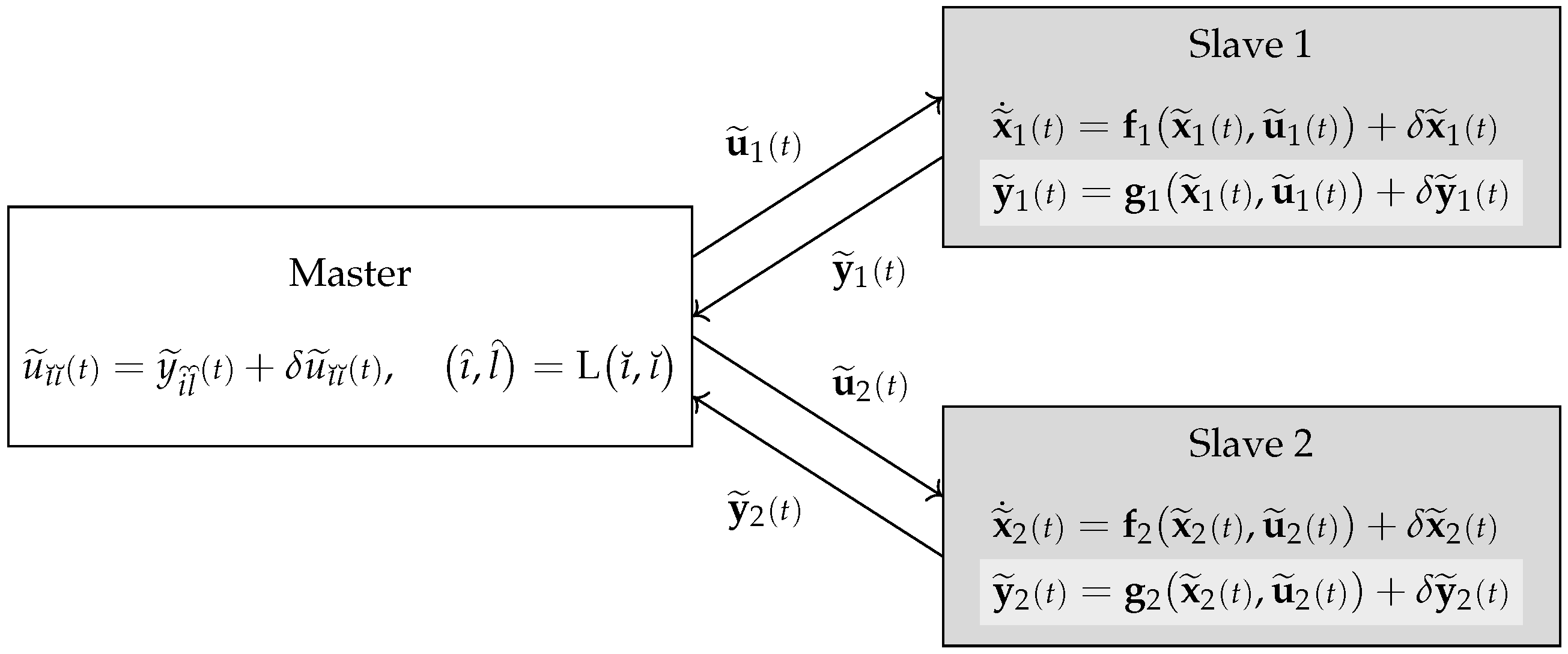
The analysis in this article and [15] is based on coupled ordinary differential equations. Coupled ordinary differential equations are a special case of differential and algebraic equations. An example of such a system is shown in Figure 1. Ordinary differential equations are used to represent the state equations of systems modeled by co-simulation slaves. Algebraic equations are divided into output and connection equations. This is performed to reflect co-simulation practice, where co-simulation slaves are typically black boxes. State and output equations are not available to the co-simulation master and are therefore colored gray in Figure 1.

This article proposes an explicit variable step co-simulation method based on numerical defect control. A co-simulation slave is responsible for generating its output signals, while the co-simulation master is responsible to solve the connection equation (Figure 1). The state and output equations are grayed out to indicate that they are usually not available to the co-simulation master. However, the output defect depends on the co-simulation step size controlled by the co-simulation master. This is why this article assumes that the output defect should be estimated by the co-simulation master and why the output equations in Figure 1 are lighter colored.

Ref. [15] provides the basis for the defect analysis of the co-simulation. This article continues that work and proposes how to adapt a step size controller [18] to co-simulation defect control. Non-iterative co-simulation in [15] is a fixed-step, multi-rate co-simulation that uses zero-order hold. This article presents a non-iterative single-rate variable-step co-simulation using higher-order interpolation.

The next section shows the basis for the analysis in this work, carried over from [15]. The defect control section introduces an explicit co-simulation variable-step method. That section shows how to calculate the connection defect and estimate the output defect. The proposed method controls the error by varying the communication step size using the PI controller. A simple application of the method is presented in the example section. This application serves to highlight some of the effects of using different orders of interpolation polynomials in co-simulation. The final section of the article contains conclusions and ideas for future work.

2. Error Bounds

This article extends the work performed in [15] with variable step co-simulation presented in the next section and experimental analysis in the following section. There, coupled ordinary differential Equation (1) and their numerical solution (2) are used to analyze numerical errors of the co-simulation. An important result of [15] is Theorem 1. It states that the global error of the co-simulation is limited when the co-simulation defect is limited. It is worth noting that a similar statement is proved in [19] for a system of differential and algebraic equations. The main difference is that algebraic equations in this article are divided into output and connection equations (Figure 1). This section repeats the expressions for coupled ordinary differential equations and the error bounds theorem from [15] (Theorem 1). Coupled ordinary differential equations are the basis for the step size analysis and Theorem 1 justifies the error control presented in the next section.

A co-simulation models a system partitioned into $N$ subsystems connected by the connection function L

$$\begin{array}{cc}\hfill & {\dot{\mathbf{x}}}_i\left(t\right)={\mathbf{f}}_i({\mathbf{x}}_i\left(t\right),{\mathbf{u}}_i\left(t\right))\hfill \end{array}$$

(1a)

$$\begin{array}{cc}\hfill & {\mathbf{y}}_i\left(t\right)={\mathbf{g}}_i({\mathbf{x}}_i\left(t\right),{\mathbf{u}}_i\left(t\right))\hfill \end{array}$$

(1b)

$$\begin{array}{cc}\hfill & {\mathbf{x}}_i\left(0\right)={\mathbf{x}}_{0i}\hfill \end{array}$$

(1c)

$$\begin{array}{cc}\hfill & u_{\stackrel{⌣}{\mathit{ı}}\stackrel{⌣}{\mathit{\iota }}}\left(t\right)=y_{\stackrel{⌢}{\mathit{i}}\stackrel{⌢}{\mathit{l}}}\left(t\right),\left(\stackrel{\mathit{⌢}}{\mathit{ı}},\stackrel{\mathit{⌢}}{\mathit{l}}\right)=\mathrm{L}\left(\stackrel{\mathit{⌣}}{\mathit{ı}},\stackrel{\mathit{⌣}}{\mathit{\iota }}\right)\hfill \end{array}$$

(1d)

where i is the subsystem index, ${\mathbf{x}}_i$ is the state signal, ${\mathbf{y}}_i$ is the output signal, ${\mathbf{u}}_i$ is the input signal, and ${\mathbf{x}}_{0i}$ is the initial state of the subsystem. The numerical solution of the system satisfies the following equations

$$\begin{array}{cc}\hfill & {\dot{\tilde{\mathbf{x}}}}_i\left(t\right)={\mathbf{f}}_i({\mathbf{x}}_i\left(t\right),{\mathbf{u}}_i\left(t\right))+\delta {\tilde{\mathbf{x}}}_i\left(t\right)\hfill \end{array}$$

(2a)

$$\begin{array}{cc}\hfill & {\tilde{\mathbf{y}}}_i\left(t\right)={\mathbf{g}}_i({\mathbf{x}}_i\left(t\right),{\mathbf{u}}_i\left(t\right))+\delta {\tilde{\mathbf{y}}}_i\left(t\right)\hfill \end{array}$$

(2b)

$$\begin{array}{cc}\hfill & {\tilde{\mathbf{x}}}_i\left(0\right)={\mathbf{x}}_{0i}\hfill \end{array}$$

(2c)

$$\begin{array}{cc}\hfill & {\tilde{u}}_{\stackrel{⌣}{\mathit{ı}}\stackrel{⌣}{\iota }}\left(t\right)={\tilde{y}}_{\stackrel{⌢}{i}\stackrel{⌢}{l}}\left(t\right)+\delta {\tilde{u}}_{\stackrel{⌣}{\mathit{ı}}\stackrel{⌣}{\iota }}\left(t\right),\left(\stackrel{⌢}{\mathit{ı}},\stackrel{⌢}{l}\right)=\mathrm{L}\left(\stackrel{⌣}{\mathit{ı}},\stackrel{⌣}{\iota }\right)\hfill \end{array}$$

(2d)

where the numerical solution of the state, output, and input signals is denoted as ${\tilde{\mathbf{x}}}_i$, ${\tilde{\mathbf{y}}}_i$, and ${\tilde{u}}_{\stackrel{⌣}{\mathit{ı}}\stackrel{⌣}{\iota }}$, respectively. The signals found by the numerical solution are assumed to be piecewise continuous. The defect introduced to the numerical solution is partitioned into integration $\delta {\tilde{\mathbf{x}}}_i$, output $\delta {\tilde{\mathbf{y}}}_i$, and connection defect $\delta {\tilde{u}}_{\stackrel{⌣}{\mathit{ı}}\stackrel{⌣}{\iota }}$. The system (1) represents the equations solved by the co-simulation and the system (2) represents the behavior of the solution obtained by the co-simulation.

The numerical solution (1) can be rewritten to

$$\begin{array}{cc}\hfill \dot{\tilde{\mathbf{x}}}\left(t\right)& =\mathbf{f}(\tilde{\mathbf{x}}\left(t\right),\tilde{\mathbf{u}}\left(t\right))+\delta \tilde{\mathbf{x}}\left(t\right)\hfill \end{array}$$

(3a)

$$\begin{array}{cc}\hfill \tilde{\mathbf{y}}\left(t\right)& =\mathbf{g}(\tilde{\mathbf{x}}\left(t\right),\tilde{\mathbf{u}}\left(t\right))+\delta \tilde{\mathbf{y}}\left(t\right)\hfill \end{array}$$

(3b)

$$\begin{array}{cc}\hfill \tilde{\mathbf{u}}\left(t\right)& =\mathbf{L}\tilde{\mathbf{y}}\left(t\right)+\delta \tilde{\mathbf{u}}\left(t\right)\hfill \end{array}$$

(3c)

where signals of all subsystems in (2) are grouped into large column vector signals

$$\begin{array}{cc}\hfill {\mathbf{x}}^T\left(t\right)& =\left[\begin{array}{cccc}{\mathbf{x}}_1^T\left(t\right)& {\mathbf{x}}_2^T\left(t\right)& \cdots & {\mathbf{x}}_N^T\left(t\right)\end{array}\right]\hfill \\ \hfill {\mathbf{y}}^T\left(t\right)& =\left[\begin{array}{cccc}{\mathbf{y}}_1^T\left(t\right)& {\mathbf{y}}_2^T\left(t\right)& \cdots & {\mathbf{y}}_N^T\left(t\right)\end{array}\right]\hfill \\ \hfill {\mathbf{u}}^T\left(t\right)& =\left[\begin{array}{cccc}{\mathbf{u}}_1^T\left(t\right)& {\mathbf{u}}_2^T\left(t\right)& \cdots & {\mathbf{u}}_N^T\left(t\right)\end{array}\right]\hfill \end{array}$$

(4)

The error of the numerical solution (3) is defined as the difference between the numerical and the analytic solution of the system (1)

$$\Delta \tilde{\mathbf{x}}\left(t\right)=\tilde{\mathbf{x}}\left(t\right)-\mathbf{x}\left(t\right),\Delta \tilde{\mathbf{y}}\left(t\right)=\tilde{\mathbf{y}}\left(t\right)-\mathbf{y}\left(t\right),\Delta \tilde{\mathbf{u}}\left(t\right)=\tilde{\mathbf{u}}\left(t\right)-\mathbf{u}\left(t\right)$$

(5)

where $\Delta \tilde{\mathbf{x}}$ is the integration error, $\Delta \tilde{\mathbf{y}}$ the output error and $\Delta \tilde{\mathbf{u}}$ the input error of the numerical solution.

Definition 1 

(Lipschitz Continuity). A function $\mathbf{f}$ is said to be Lipschitz continuous if there exist constant $K_{\mathbf{f}}>0$ such that for all ${\mathbf{x}}_1,{\mathbf{x}}_2\in {\mathbb{R}}^{\left|\mathbf{x}\right|}$:

$$∥\mathbf{f}\left({\mathbf{x}}_2\right)-\mathbf{f}\left({\mathbf{x}}_1\right)∥⩽K_{\mathbf{f}}∥{\mathbf{x}}_2-{\mathbf{x}}_1∥$$

(6)

The constant $K_{\mathbf{f}}$ is called the Lipschitz constant of the function $\mathbf{f}$.

Definition 1 introduces Lipschitz continuity, which is used to describe the conditions for the uniqueness of the solution for (1) [15]. It is used to formulate Assumption 1 and Theorem 1.

Assumption 1. 

Assume that there exists a Lipschitz continuous function $\mathbf{G}$ that explicitly calculates the input signals

$$\tilde{\mathbf{u}}\left(t\right)=\mathbf{G}(\tilde{\mathbf{x}}\left(t\right),\delta \tilde{\mathbf{y}}\left(t\right),\delta \tilde{\mathbf{u}}\left(t\right))$$

(7)

Assume that the aggregated state transition function $\mathbf{f}$ (3a) is Lipschitz continuous. Assume that the aggregated output function $\mathbf{g}$ (3b) is Lipschitz continuous. Assume that the numerical solution (2) is continuous in every subinterval$(t_{\kappa -1},t_{\kappa }]$.

Theorem 1 

(Error Bounds = Theorem 2.12 in [15]). Suppose Assumption (1) holds. Then, the integration error is limited

$$\parallel \Delta \tilde{\mathbf{x}}\left(t\right)\parallel ⩽e^{K_{\mathbf{f}}(t-t_0)}\parallel \Delta \tilde{\mathbf{x}}\left(t_0\right)\parallel +\frac{1}{K_{\mathbf{f}}}\left(e^{K_{\mathbf{f}}(t-t_0)}-1\right){\delta }^{\left(t_0,t\right]}$$

(8)

the input error satisfies is limited

$$\begin{array}{cc}\hfill \parallel \Delta \tilde{\mathbf{u}}\left(t\right)\parallel ⩽& K_{\mathbf{G}}{e}^{K_{\mathbf{f}}(t-t_0)}\parallel \Delta \tilde{\mathbf{x}}\left(t_0\right)\parallel +\frac{K_{\mathbf{G}}}{K_{\mathbf{f}}}\left(e^{K_{\mathbf{f}}(t-t_0)}-1\right){\delta }^{\left(t_0,t\right]}\hfill \\ \hfill & +K_{\mathbf{G}}\parallel \delta \tilde{\mathbf{y}}\left(t\right)\parallel +K_{\mathbf{G}}\parallel \delta \tilde{\mathbf{u}}\left(t\right)\parallel \hfill \end{array}$$

(9)

and the output error satisfies is limited

$$\begin{array}{cc}\hfill \parallel \Delta \tilde{\mathbf{y}}\left(t\right)\parallel ⩽& K_{\mathbf{g}}\left(1+K_{\mathbf{G}}\right)e^{K_{\mathbf{f}}(t-t_0)}\parallel \Delta \tilde{\mathbf{x}}\left(t_0\right)\parallel \hfill \\ \hfill & +\frac{K_{\mathbf{g}}}{K_{\mathbf{f}}}\left(1+K_{\mathbf{G}}\right)\left(e^{K_{\mathbf{f}}(t-t_0)}-1\right){\delta }^{\left(t_0,t\right]}\hfill \\ \hfill & +\left(1+K_{\mathbf{g}}{K}_{\mathbf{G}}\right)\parallel \delta \tilde{\mathbf{y}}\left(t\right)\parallel +K_{\mathbf{g}}{K}_{\mathbf{G}}\parallel \delta \tilde{\mathbf{u}}\left(t\right)\parallel \hfill \end{array}$$

(10)

In [15], it is shown that Theorem 1 requires the same conditions as the uniqueness of the solution for (1). In addition, the numerical solution obtained by co-simulation (2) must be piecewise continuous. This theorem provides the justification for the defect control presented next.

3. Defect Control

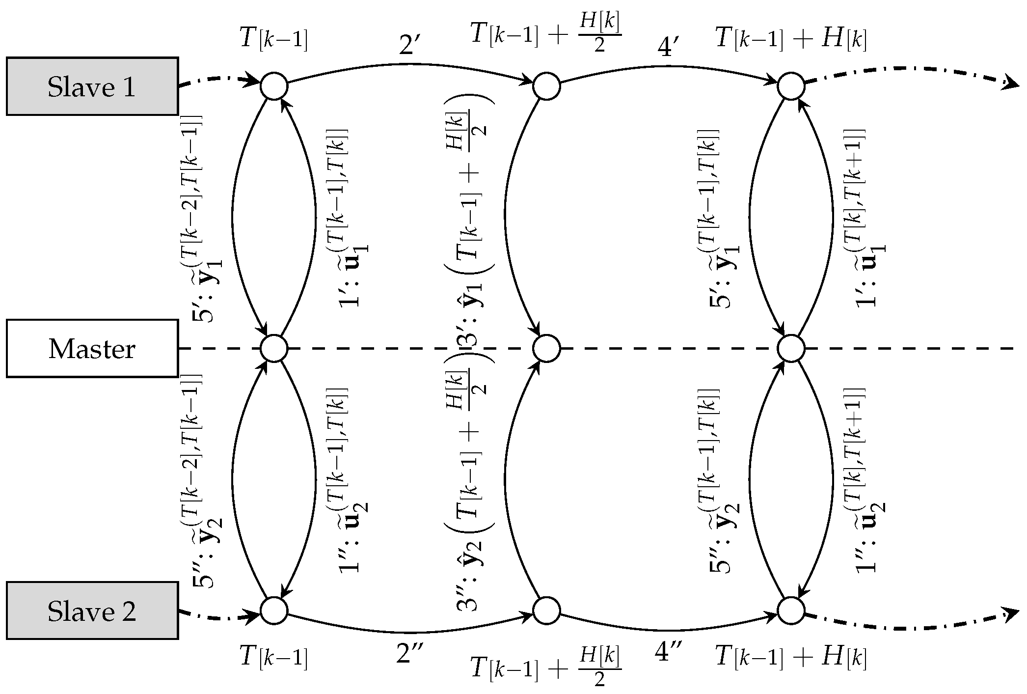
Theorem 1 suggests that the step size control of the co-simulation defect can be used to limit the global error of the co-simulation. According to [3], a communication step size is the “distance between two subsequent communication points (also known as sampling rate or macro step size)”, where communication points are “time grid for data exchange between master and slaves in a co-simulation environment (also known as sampling points or synchronization points)”. This section describes how to control the communication step size of a slave using a non-iterative variant of the Jacobi co-simulation method (Algorithm 1). The proposed co-simulation method is shown in Figure 2. The variable-step variant of the method generates a sequence of communication step sizes $H:\mathbb{N}\to {\mathbb{R}}_{⩾0}$ with the explicit version of the PI control procedure introduced in [18]. The defect controlled by the proposed method is based on the connection defect (2d) and/or the output defect (2b).

The numerical defect must be limited to ensure that the co-simulation error is limited. Theorems 2 and 3 show that the defect can be limited by reducing the communication step size. This section shows how to calculate the connection defect and estimate the output defect. Theorem 4 shows that the output defect estimate used is asymptotically correct.

The sequence of communication points $T:{\mathbb{N}}_0\to {\mathbb{R}}_{⩾0}$ is determined by the communication step sizes

$$T\left[k\right]=T\left[k-1\right]+H\left[k\right]$$

(11)

The sequence of points $t_{\kappa }$ at which a numeric solution discontinuity can occur is marked differently than the sequence of communication points $T\left[k\right]$. The reason is that discontinuities in the numeric solution may occur during slave integration. Each slave can perform the integration with different individual integration steps (sometimes referred to as a micro step size ). It is assumed that the internal solver of the slave takes over the responsibility for the control of the integration step size. Control of the integration step size may be used to reduce the integration error [16,17]. Theorem 1 suggests that integration defect reduction is an important factor for the quality of co-simulation. This article focuses on controlling the size of the communication step with respect to output and connection defects. This choice respects the black box character of co-simulation slaves (Figure 1) and leaves the integration defects in the responsibility of internal slave solvers.

Co-simulation is the simulation of a continuous time model with a computer, a discrete system. The co-simulation generates samples of the signal and its derivatives at communication points. This description is consistent with [3]. The reconstruction of output signals from such samples can be obtained using the Taylor polynomial

$${\tilde{\mathbf{y}}}_i^{\left(T\left[k-1\right],T\left[k\right]\right]}\left(t\right)=\sum _{n=0}^{n_i}\frac{{\mathrm{d}}^n{\tilde{\mathbf{y}}}_i^{\left(T\left[k-1\right],T\left[k\right]\right]}}{{\mathrm{dt}}^n}\left(T\left[k\right]\right)\frac{{\left(t-T\left[k\right]\right)}^n}{n!}$$

(12)

where the samples of the output signal and its derivatives are determined by the co-simulation slave. The output signal of the $i^{\mathrm{th}}$ co-simulation slave is a piecewise polynomial signal

$${\tilde{\mathbf{y}}}_i\left(t\right)={\tilde{\mathbf{y}}}_i^{\left(T\left[k-1\right],T\left[k\right]\right]}\left(t\right),T\left[k-1\right]<t⩽T\left[k\right]$$

(13)

The inputs of the $i^{\mathrm{th}}$ co-simulation slave are extrapolated with the following polynomial

$${\tilde{\mathbf{u}}}_i^{\left(T\left[k-1\right],T\left[k\right]\right]}\left(t\right)=\sum _{m=0}^{m_i}\frac{{\mathrm{d}}^m{\tilde{\mathbf{u}}}_i^{\left(T\left[k-1\right],T\left[k\right]\right]}}{{\mathrm{dt}}^m}\left(T\left[k-1\right]\right)\frac{{\left(t-T\left[k-1\right]\right)}^m}{m!}$$

(14)

where the samples of the input signal and its derivatives are determined by the co-simulation master. A non-iterative Jacobi co-simulation master (Figure 2) determines the input signals in the $k^{\mathrm{th}}$ step with the connected output signals from the ${(k-1)}^{st}$ step

$$\begin{array}{cc}\hfill \frac{{\mathrm{d}}^m{\tilde{u}}_{\stackrel{⌣}{\mathit{ı}}\stackrel{⌣}{\iota }}^{\left(T\left[k\right],T\left[k+1\right]\right]}}{{\mathrm{dt}}^m}\left(T\left[k-1\right]\right)=& \frac{{\mathrm{d}}^m{\tilde{y}}_{\stackrel{⌢}{i}\stackrel{⌢}{l}}^{\left(T\left[k-2\right],T\left[k-1\right]\right]}}{{\mathrm{dt}}^m}\left(T\left[k-1\right]\right),\hfill \\ \hfill & \left(\stackrel{⌢}{\mathit{ı}},\stackrel{⌢}{l}\right)=\mathrm{L}\left(\stackrel{⌣}{\mathit{ı}},\stackrel{⌣}{\iota }\right),m⩽m_{\stackrel{⌣}{\mathit{ı}}},m⩽n_{\stackrel{⌢}{\mathit{ı}}}\hfill \end{array}$$

(15)

The input signal of the $i^{\mathrm{th}}$ co-simulation slave is a piecewise polynomial signal

$${\tilde{\mathbf{u}}}_i\left(t\right)={\tilde{\mathbf{u}}}_i^{\left(T\left[k-1\right],T\left[k\right]\right]}\left(t\right),T\left[k-1\right]<t⩽T\left[k\right]$$

(16)

The connection defect (2d) can be calculated by comparing the extrapolation polynomials for the output (12) and input (14) signals, i.e.,

$$\delta {\tilde{u}}_{\stackrel{⌣}{\mathit{ı}}\stackrel{⌣}{\iota }}^{\left(T\left[k-1\right],T\left[k\right]\right]}\left(t\right)={\tilde{u}}_{\stackrel{⌣}{\mathit{ı}}\stackrel{⌣}{\iota }}^{\left(T\left[k-1\right],T\left[k\right]\right]}\left(t\right)-{\tilde{y}}_{\stackrel{⌢}{\mathit{i}}\stackrel{⌢}{\mathit{l}}}^{\left(T\left[k-1\right],T\left[k\right]\right]}\left(t\right),\left(\stackrel{⌢}{\mathit{ı}},\stackrel{⌢}{\mathit{l}}\right)=\mathrm{L}\left(\stackrel{⌣}{\mathit{ı}},\stackrel{⌣}{\iota }\right)$$

(17)

where individual scalar signals are selected according to the connection function.

This article assumes that the output signal and all its derivatives are perfectly sampled, i.e., the output defect can only deviate from zero between the communication points

$$\frac{{\mathrm{d}}^n{\tilde{\mathbf{y}}}_i^{\left(T\left[k-1\right],T\left[k\right]\right]}}{{\mathrm{dt}}^n}\left(T\left[k\right]\right)={\left.\frac{{\mathrm{d}}^n{\mathbf{g}}_i\left({\tilde{\mathbf{x}}}_i\left(t\right),{\tilde{\mathbf{u}}}_i\left(t\right)\right)}{{\mathrm{dt}}^n}\right|}_{t=T\left[k\right]},n=0,\dots ,n_i$$

(18)

Lemma 1. 

Assume that the numerical solution for the input signals is bounded $\parallel {\tilde{\mathbf{u}}}_{\stackrel{⌢}{\mathit{ı}}}\left(t\right)\parallel ⩽B_{{\tilde{\mathbf{u}}}_{\stackrel{⌢}{\mathit{ı}}}}$, the numerical solution for the state signal is bounded $\parallel {\tilde{\mathbf{x}}}_{\stackrel{⌢}{\mathit{ı}}}\left(t\right)\parallel ⩽B_{{\tilde{\mathbf{x}}}_{\stackrel{⌢}{\mathit{ı}}}}$, the integration defects are $\delta {\tilde{\mathbf{x}}}_{\stackrel{⌢}{\mathit{ı}}}\left(t\right)=\mathcal{O}\left(H^{N_i}\left[k\right]\right)$, and the state transition function ${\mathbf{f}}_{\stackrel{⌢}{\mathit{ı}}}$ is Lipschitz continuous (Definition 1). Then

$$\underset{H\left[k\right]\to 0}{lim}∥{\tilde{\mathbf{x}}}_{\stackrel{⌢}{\mathit{ı}}}\left(T\left[k\right]\right)-{\tilde{\mathbf{x}}}_{\stackrel{⌢}{\mathit{ı}}}\left(T\left[k-1\right]\right)∥=0$$

(19)

Proof. 

Since $\delta {\tilde{\mathbf{x}}}_{\stackrel{⌢}{\mathit{ı}}}\left(t\right)=\mathcal{O}\left(H^{N_i}\left[k\right]\right)$ there exists $C,H_0\in {\mathbb{R}}_{>0}$ such that for all $H\left[k\right]⩽H_0$

$$\parallel \delta {\tilde{\mathbf{x}}}_{\stackrel{⌢}{\mathit{ı}}}\left(t\right)\parallel ⩽C{H}_0^{N_i}$$

(20)

By the integration of (2a)

$${\tilde{\mathbf{x}}}_{\stackrel{⌢}{\mathit{ı}}}\left(T\left[k\right]\right)-{\tilde{\mathbf{x}}}_{\stackrel{⌢}{\mathit{ı}}}\left(T\left[k-1\right]\right)=\underset{T\left[k-1\right]}{\overset{T\left[k\right]}{\int }}\mathbf{f}\left({\tilde{\mathbf{x}}}_{\stackrel{⌢}{\mathit{ı}}}\left(\tau \right),{\tilde{\mathbf{u}}}_{\stackrel{⌢}{\mathit{ı}}}\left(\tau \right)\right)+\delta {\tilde{\mathbf{x}}}_{\stackrel{⌢}{\mathit{ı}}}\left(\tau \right)\mathrm{d}\tau$$

(21)

the following inequality is obtained

$$∥{\tilde{\mathbf{x}}}_{\stackrel{⌢}{\mathit{ı}}}\left(T\left[k\right]\right)-{\tilde{\mathbf{x}}}_{\stackrel{⌢}{\mathit{ı}}}\left(T\left[k-1\right]\right)∥⩽\underset{T\left[k-1\right]}{\overset{T\left[k-1\right]+H\left[k\right]}{\int }}{K}_{\mathbf{f}}{B}_{{\tilde{\mathbf{x}}}_{\stackrel{⌢}{\mathit{ı}}}}+K_{\mathbf{f}}{B}_{{\tilde{\mathbf{u}}}_{\stackrel{⌢}{\mathit{ı}}}}+C{H}_0^{N_i}\mathrm{d}\tau$$

(22)

The statement of the lemma (19) follows from the previous inequality

$$∥{\tilde{\mathbf{x}}}_{\stackrel{⌢}{\mathit{ı}}}\left(T\left[k\right]\right)-{\tilde{\mathbf{x}}}_{\stackrel{⌢}{\mathit{ı}}}\left(T\left[k-1\right]\right)∥⩽\left(K_{\mathbf{f}}{B}_{{\tilde{\mathbf{x}}}_{\stackrel{⌢}{\mathit{ı}}}}+K_{\mathbf{f}}{B}_{{\tilde{\mathbf{u}}}_{\stackrel{⌢}{\mathit{ı}}}}+C{H}_0^{N_i}\right)H\left[k\right]$$

(23)

   □

Theorem 2 

(Connection defect). Assume that the numerical solution for the input signals is bounded $\parallel {\tilde{\mathbf{u}}}_{\stackrel{⌢}{\mathit{ı}}}\left(t\right)\parallel ⩽B_{{\tilde{\mathbf{u}}}_{\stackrel{⌢}{\mathit{ı}}}}$, the numerical solution for the state signal is bounded $\parallel {\tilde{\mathbf{x}}}_{\stackrel{⌢}{\mathit{ı}}}\left(t\right)\parallel ⩽B_{{\tilde{\mathbf{x}}}_{\stackrel{⌢}{\mathit{ı}}}}$, the integration defects are $\delta {\tilde{\mathbf{x}}}_{\stackrel{⌢}{\mathit{ı}}}\left(t\right)=\mathcal{O}\left(H^{N_{\stackrel{⌢}{\mathit{ı}}}}\left[k\right]\right)$, the state transition function ${\mathbf{f}}_{\stackrel{⌢}{\mathit{ı}}}$ is Lipschitz continuous (Definition 1), the output function of the ${\stackrel{⌢}{\mathit{ı}}}^{th}$ subsystem is

$${\mathbf{g}}_{\stackrel{⌢}{\mathit{ı}}}({\tilde{\mathbf{x}}}_{\stackrel{⌢}{\mathit{ı}}}\left(t\right),{\tilde{\mathbf{u}}}_{\stackrel{⌢}{\mathit{ı}}}\left(t\right))={\mathbf{g}}_{\stackrel{⌢}{\mathit{ı}}}\left({\tilde{\mathbf{x}}}_{\stackrel{⌢}{\mathit{ı}}}\left(t\right)\right)$$

(24)

and the step sizes of connected simulators $\stackrel{⌢}{i},\stackrel{⌣}{\mathit{ı}}\in IF$. The connection defect (2d) of a numerical solution converges in terms of the communication step size

$$\underset{H\left[k\right]\to 0}{lim}\left(\delta {\tilde{u}}_{\stackrel{⌣}{\mathit{ı}}\stackrel{⌣}{\iota }}^{\left(T\left[k-1\right],T\left[k\right]\right]}\left(t\right)\right)=0$$

(25)

Proof. 

From (14)–(18) and (24) it follows that

$$\begin{array}{cc}\hfill \delta {\tilde{u}}_{\stackrel{⌣}{\mathit{ı}}\stackrel{⌣}{\iota }}^{\left(T\left[k-1\right],T\left[k\right]\right]}\left(t\right)=& \sum _{m=0}^{min(m_{\stackrel{⌣}{\mathit{ı}}},n_{\stackrel{⌢}{\mathit{ı}}})}{\left.\frac{{\mathrm{d}}^m{g}_{\stackrel{⌢}{\mathit{ı}}\stackrel{⌢}{l}}\left({\tilde{\mathbf{x}}}_{\stackrel{⌢}{\mathit{ı}}}\left(t\right)\right)}{{\mathrm{dt}}^m}\right|}_{t=T\left[k-1\right]}\frac{{\left(t-T\left[k-1\right]\right)}^m}{m!}\hfill \\ \hfill & -\sum _{n=0}^{n_{\stackrel{⌢}{\mathit{ı}}}}{\left.\frac{{\mathrm{d}}^n{g}_{\stackrel{⌢}{\mathit{ı}}\stackrel{⌢}{l}}\left({\tilde{\mathbf{x}}}_{\stackrel{⌢}{\mathit{ı}}}\left(t\right)\right)}{{\mathrm{dt}}^n}\right|}_{t=T\left[k\right]}\frac{{\left(t-T\left[k\right]\right)}^n}{n!}\hfill \\ \hfill =& g_{\stackrel{⌢}{\mathit{ı}}\stackrel{⌢}{l}}\left({\tilde{\mathbf{x}}}_{\stackrel{⌢}{\mathit{ı}}}\left(T\left[k-1\right]\right)\right)-g_{\stackrel{⌢}{\mathit{ı}}\stackrel{⌢}{l}}\left({\tilde{\mathbf{x}}}_{\stackrel{⌢}{\mathit{ı}}}\left(T\left[k\right]\right)\right)+\mathcal{O}\left(H\left[k\right]\right)\hfill \end{array}$$

(26)

where $\left(\stackrel{⌢}{\mathit{ı}},\stackrel{⌢}{l}\right)=\mathrm{L}\left(\breve{\mathit{ı}},\breve{\iota }\right)$. Since ${\mathbf{g}}_{\stackrel{⌢}{\mathit{ı}}}$ is Lipschitz continuous it follows that

$$∥g_{\stackrel{⌢}{\mathit{ı}}\stackrel{⌢}{l}}\left({\tilde{\mathbf{x}}}_{\stackrel{⌢}{\mathit{ı}}}\left(T\left[k-1\right]\right)\right)-g_{\stackrel{⌢}{\mathit{ı}}\stackrel{⌢}{l}}\left({\tilde{\mathbf{x}}}_{\stackrel{⌢}{\mathit{ı}}}\left(T\left[k\right]\right)\right)∥⩽K_{{\mathbf{g}}_{\stackrel{⌢}{i}}}∥{\tilde{\mathbf{x}}}_{\stackrel{⌢}{\mathit{ı}}}\left(T\left[k-1\right]\right)-{\tilde{\mathbf{x}}}_{\stackrel{⌢}{\mathit{ı}}}\left(T\left[k\right]\right)∥$$

(27)

The statement of the theorem follows from Lemma 1, (26) and (27).    □

Theorem 2 specifies the conditions under which the connection defect converges with respect to the communication step size. A number of simplifications are adopted to prove Theorem 2. In (26), the higher order terms are ignored to simplify the proof. The goal was to prove that the connection defect was converging in terms of communication step size, rather than finding the smallest limit. The next section shows the order of convergence of the connection defect in a simple example. Bounded inputs and state signals are reasonable assumptions for a stable system and a stable co-simulation. The assumptions (24), however, restrict the models used to those that have no direct output dependency on input signals. If this simplification is not applied, it is possible to construct a system with an algebraic loop that makes the co-simulation unstable. The subject of future work will be to analyze how some or all of these simplifications can be discarded or at least relaxed.

Theorem 3 

(Output defect). Suppose the function ${\mathbf{g}}_i$ is continuously differentiable and the calculated state signal ${\tilde{\mathbf{x}}}_i$ is continuously differentiable. Then, the output defect (2b) is

$$\delta {\tilde{\mathbf{y}}}_i\left(t\right)=\mathcal{O}\left(H^{n_i+1}\left[k\right]\right)$$

(28)

Proof. 

From (14) and the fact that ${\mathbf{g}}_i$ and ${\tilde{\mathbf{x}}}_i$ are continuously differentiable, it follows that

$$\mathbf{g}\left({\tilde{\mathbf{x}}}_i\left(t\right),{\tilde{\mathbf{u}}}_i\left(t\right)\right)=\sum _{n=0}^{n_i}{\left.\frac{{\mathrm{d}}^{n_i}\mathbf{g}\left({\tilde{\mathbf{x}}}_i\left(\tau \right),{\tilde{\mathbf{u}}}_i\left(\tau \right)\right)}{\mathrm{d}{\tau }^{n_i}}\right|}_{\tau =T\left[k\right]}\frac{{\left(t-T\left[k\right]\right)}^n}{n!}+\mathcal{O}\left(H^{n_i+1}\left[k\right]\right)$$

(29)

for $T\left(k-1\right)<t⩽T\left[k\right]$ The expression (28) follows from (2b), (12) and (18).    □

Theorem 3 shows that the output defect can be controlled by reducing the communication step size. Theorem 2 and Theorem 3 justify the communication step size control. Numerical solvers are expected to minimize the remaining component of the numerical defect, the integration defect (2a). The rest of the section analyzes how to estimate the output defect.

For the purpose of estimating the output defect between the communication points, a Hermite interpolation polynomial [20] is łintroduced

$${\widehat{\mathbf{y}}}_i^{\left(T\left[k-1\right],T\left[k\right]\right]}\left(t\right)={\tilde{\mathbf{y}}}_i\left(t\right)+\frac{{\left(T\left[k\right]-t\right)}^{n_i+1}}{{\left(0.5H\left[k\right]\right)}^{n_i+1}}\left[{\mathbf{g}}_i\left({\tilde{\mathbf{x}}}_i\left(T\left[k\right]-\frac{H\left[k\right]}{2}\right),{\tilde{\mathbf{u}}}_i\left(T\left[k\right]-\frac{H\left[k\right]}{2}\right)\right)-{\tilde{\mathbf{y}}}_i\left(T\left[k\right]-\frac{H\left[k\right]}{2}\right)\right]$$

(30)

A Hermite interpolation polynomial is consistent with multiple samples of the signals and their derivatives. The polynomial used in this paper is consistent with signal values at two communication points and signal derivatives at the later point

$$\begin{array}{cc}\hfill & {\widehat{\mathbf{y}}}_i^{\left(T\left[k-1\right],T\left[k\right]\right]}\left(T\left[k\right]-\frac{H\left[k\right]}{2}\right)={\mathbf{g}}_i\left({\tilde{\mathbf{x}}}_i\left(T\left[k\right]-\frac{H\left[k\right]}{2}\right),{\tilde{\mathbf{u}}}_i\left(T\left[k\right]-\frac{H\left[k\right]}{2}\right)\right)\hfill \\ \hfill & \frac{{\mathrm{d}}^n{\widehat{\mathbf{y}}}_i^{\left(T\left[k-1\right],T\left[k\right]\right]}}{{\mathrm{dt}}^n}\left(T\left[k\right]\right)={\left.\frac{{\mathrm{d}}^n{\mathbf{g}}_i\left({\tilde{\mathbf{x}}}_i\left(t\right),{\tilde{\mathbf{u}}}_i\left(t\right)\right)}{{\mathrm{dt}}^n}\right|}_{t=T\left[k\right]},n=0,\dots ,n_i\hfill \end{array}$$

(31)

The Hermite interpolation polynomial is used to obtain an asymptotically correct estimate of the output defect.

Theorem 4 

(Estimate of the Output Defect). The estimation of the output defect is defined as the difference between interpolation polynomials (30) and (12)

$$\widehat{\delta }{\tilde{\mathbf{y}}}_i^{\left(T\left[k-1\right],T\left[k\right]\right]}\left(t\right)={\tilde{\mathbf{y}}}_i^{\left(T\left[k-1\right],T\left[k\right]\right]}\left(t\right)-{\widehat{\mathbf{y}}}_i^{\left(T\left[k-1\right],T\left[k\right]\right]}\left(t\right)$$

(32)

Suppose the function ${\mathbf{g}}_i$ is $n_i+1$ times continuously differentiable on the interval $t\in \left(T\left[k-1\right],T\left[k\right]\right]$ and

$${\tilde{\mathbf{x}}}_i^{\left(T\left[k-1\right],T\left[k\right]\right]}\left(t\right)=\sum _{n=0}^{n_i+1}\frac{{\mathrm{d}}^n{\tilde{\mathbf{x}}}_i}{{\mathrm{dt}}^n}\left(T\left[k\right]\right)\frac{{\left(t-T\left[k\right]\right)}^n}{n!}+\mathcal{O}\left(H^{n_i+2}\left[k\right]\right)$$

(33)

Then, the estimate of the output defect (32) is asymptotically correct, i.e., for each $\alpha \in \left(0,1\right)$

$$\underset{H\left[k\right]\to 0}{lim}\frac{\widehat{\delta }{\tilde{\mathbf{y}}}_i^{\left(T\left[k-1\right],T\left[k\right]\right]}\left(t\right)}{\delta {\tilde{\mathbf{y}}}_i^{\left(T\left[k-1\right],T\left[k\right]\right]}\left(t\right)}=1,t=T\left[k-1\right]+\alpha H\left[k\right]$$

(34)

Proof. 

Since ${\mathbf{g}}_i$ is continuously differentiable, it is also Lipschitz continuous. Lipschitz continuity and (33) imply

$${\mathbf{g}}_i\left({\tilde{\mathbf{x}}}_i^{\left(T\left[k-1\right],T\left[k\right]\right]}\left(t\right),{\tilde{\mathbf{u}}}_i^{\left(T\left[k-1\right],T\left[k\right]\right]}\left(t\right)\right)=\sum _{n=0}^{n_i+1}\left[{\left.\frac{{\mathrm{d}}^n{\mathbf{g}}_i\left({\tilde{\mathbf{x}}}_i\left(t\right),{\tilde{\mathbf{u}}}_i\left(t\right)\right)}{{\mathrm{dt}}^n}\right|}_{t=T\left[k\right]}\frac{{\left(t-T\left[k\right]\right)}^n}{n!}\right]+\mathcal{O}\left(H^{n_i+2}\left[k\right]\right)$$

(35)

The output defect (3b) is the difference between the numerical output signal (12) and the output signal without defect (35). The output defect on the interval $\left(T\left[k-1\right],T\left[k\right]\right]$ is equal to

$$\delta {\tilde{\mathbf{y}}}_i\left(t\right)={\tilde{\mathbf{y}}}_i\left(t\right)-{\mathbf{g}}_i\left({\tilde{\mathbf{x}}}_i\left(t\right),{\tilde{\mathbf{u}}}_i\left(t\right)\right)={\left.\frac{{\mathrm{d}}^{n_i+1}{\mathbf{g}}_i\left({\tilde{\mathbf{x}}}_i\left(t\right),{\tilde{\mathbf{u}}}_i\left(t\right)\right)}{{\mathrm{dt}}^{n_i+1}}\right|}_{t=T\left[k\right]}\frac{{\left(t-T\left[k\right]\right)}^{n_i+1}}{(n_i+1)!}+\mathcal{O}\left(H^{n_i+2}\left[k\right]\right)$$

(36)

The estimate of the output defect on the interval $\left(T\left[k-1\right],T\left[k\right]\right]$ is equal to

$$\begin{array}{cc}\hfill \widehat{\delta }{\tilde{\mathbf{y}}}_i^{\left(T\left[k-1\right],T\left[k\right]\right]}\left(t\right)& =\frac{{\left(T\left[k\right]-t\right)}^{n_i+1}}{{\left(0.5H\left[k\right]\right)}^{n_i+1}}\left[{\mathbf{g}}_i\left({\tilde{\mathbf{x}}}_i\left(T\left[k\right]-\frac{H\left[k\right]}{2}\right),{\tilde{\mathbf{u}}}_i\left(T\left[k\right]-\frac{H\left[k\right]}{2}\right)\right)-{\tilde{\mathbf{y}}}_i\left(T\left[k\right]-\frac{H\left[k\right]}{2}\right)\right]\hfill \\ \hfill & =\frac{{\left(T\left[k\right]-t\right)}^{n_i+1}}{{\left(0.5H\left[k\right]\right)}^{n_i+1}}\left[{\left.\frac{{\mathrm{d}}^{n_i+1}{\mathbf{g}}_i\left({\tilde{\mathbf{x}}}_i\left(t\right),{\tilde{\mathbf{u}}}_i\left(t\right)\right)}{{\mathrm{dt}}^{n_i+1}}\right|}_{t=T\left[k\right]}\frac{{\left(-0.5H\left[k\right]\right)}^{n_i+1}}{(n_i+1)!}+\mathcal{O}\left(H{\left[k\right]}^{n_i+2}\right)\right]\hfill \\ \hfill & ={\left.\frac{{\mathrm{d}}^{n_i+1}{\mathbf{g}}_i\left({\tilde{\mathbf{x}}}_i\left(t\right),{\tilde{\mathbf{u}}}_i\left(t\right)\right)}{{\mathrm{dt}}^{n_i+1}}\right|}_{t=T\left[k\right]}\frac{{\left(t-T\left[k\right]\right)}^{n_i+1}}{(n_i+1)!}+\mathcal{O}\left(H^{n_i+2}\left[k\right]\right)\hfill \end{array}$$

(37)

The Equation (34) follows directly from (36) and (37).    □

The output defect estimate (32) is obtained by adding communication points during co-simulation. The additional points are added in the middle of the interval $\left(T\left[k-1\right],T\left[k\right]\right]$ shown in Figure 2. These points are used to obtain a higher order interpolation polynomial (30) for use in the output defect estimate. Theorem 4 gives the conditions (33) under which the output defect estimate (32) is asymptotically correct. The integration should have a higher order of local error than the order of the output interpolation polynomial (12).

The connection defect calculation (17) and the output defect estimate (32) are used to define the controlled co-simulation defect

$$ϵ\left[k\right]=max\left(\underset{i,j}{max}\left(\underset{T\left[k-1\right]<t⩽T\left[k\right]}{RMS}\left(\delta {\tilde{u}}_{ij}\right)\right),\underset{i,j}{max}\left(\underset{T\left[k-1\right]<t⩽T\left[k\right]}{RMS}(\widehat{\delta }{\tilde{y}}_{ij})\right)\right)$$

(38)

The calculation of the co-simulation defect is used in a step size control approach similar to the one introduced in [18]. The approach uses a PI controller for the logarithm of an error measurement

$$\begin{array}{cc}\hfill & e\left[k\right]=log\left(tol\right)-log\left(ϵ\left[k\right]\right)\hfill \\ \hfill & I^{\prime }\left[k\right]=I\left[k-1\right]+K_{I}e\left[k\right]\hfill \\ \hfill & H^{\prime }\left[k\right]=exp\left(I^{\prime }\left[k\right]+K_{P}e\left[k\right]\right)\hfill \\ \hfill & H\left[k\right]=\left\{\begin{array}{cc}{\theta }_{max}H\left[k-1\right],\hfill & H^{\prime }\left[k\right]>{\theta }_{max}H\left[k-1\right]\hfill \\ H^{\prime }\left[k\right],\hfill & otherwise\hfill \end{array}\right.\hfill \\ \hfill & I\left[k\right]=I^{\prime }\left[k\right]+log\left(H\left[k\right]\right)-log\left(H^{\prime }\left[k\right]\right)\hfill \\ \hfill & H\left[1\right]=H_1,I\left[1\right]=log\left(H_1\right)\hfill \end{array}$$

(39)

where $ϵ:\mathbb{N}\to \mathbb{R}$ is the controlled error approximation. Such a method has already been used for co-simulation [21]. The difference to the method presented in this article is the controlled error estimate. In [21], the authors have used an explicit step size control procedure to control the local co-simulation error of the output signal. In this article, the method controls the maximum of the connection defect and the output defect estimate (38).

The co-simulation method used for demonstrating the communication step size control is defined in Algorithm 1. It is also shown in Figure 2 to simplify the introduction. Like any other co-simulation master, the method solves the connection Equation (1d) and controls the execution of the co-simulation slaves. The connection equation is solved by the assignment of input signal derivatives (15). The presented co-simulation method allows a parallel execution with a distribution of the calculation performed in for-loops. The communication step sizes are controlled using the PI controller (39) to keep the co-simulation defect (38) constant.

4. Numerical Example

This section presents an example of using the proposed variable-step co-simulation method (Algorithm 1). The example system is a two mass oscillator that is commonly used to benchmark co-simulation master algorithms [6,21,22,23,24,25]. The slaves are implemented in the C programming language using Functional Mock-up Interface (FMI) [3,4]. The proposed connection defect calculation (17) and the output defect estimation (32) are illustrated in this example.

Algorithm 1 The pseudocode describes a non-iterative Jacobi co-simulation method. In the variable-step variant, the step size $H\left[k\right]$ is computed with the PI controller (17), (32), (38) and (39). In the fixed-step variant, the step size is constant $H\left[k\right]=H\left[k-1\right]=H_1$.

Require:  a partitioned system (1) without algebraic loops, an initial step size $H_1$, defect tolerance $tol$ 1: $k:=0$, $T\left[k\right]:=0$, $H\left[1\right]=H_1$ 2: calculate the initial output signals by solving the Equations (1b) and (1d) 3: repeat 4:     $k:=k+1$ 5:     for $i\leftarrow 1$ to N do 6:          assign the input signals (15) 7:     for $i\leftarrow 1$ to N do 8:          integrate the Equation (1a) on the interval $\left(T\left[k-1\right],T\left[k-1\right]+\frac{H\left[k\right]}{2}\right]$ 9:     for $i\leftarrow 1$ to N do 10:          obtain the output signal samples at $T\left[k-1\right]+\frac{H\left[k\right]}{2}$ 11:     for $i\leftarrow 1$ to N do 12:          integrate the Equation (1a) on the interval $\left(T\left[k-1\right]+\frac{H\left[k\right]}{2},T\left[k\right]\right]$ 13:     for $i\leftarrow 1$ to N do 14:          obtain the output signal samples at $T\left[k\right]$ 15:     compute $H\left[k\right]$ 16:     $T\left[k\right]:=T\left[k-1\right]+H\left[k\right]$ 17: until  $T\left[k\right]⩽t_{end}$

The algorithms presented in this article and the code used to generate the results in this section are published at [26]. The models are implemented in C, the algorithms are implemented in C++, and the figures are created in Python. In the repository [26] an interested reader can find

• a C++ implementation of Algorithm 1 in the template function
  fmi::jacobi_co_simulation (src/fmi.h),
• an implementation of the step size controller (39) in the method VariableStepSize::next (src/fmi.cpp),
• an implementation of the Hermite polynomial calculation (30) in the method FMU::get_hermite (src/fmi.cpp),
• an implementation of the output defect calculation in the function fmi::calculate _output_defects (src/fmi.cpp),
• an implementation of connection defect calculation in the function fmi::calculate _connection_defects (src/fmi.cpp),
• an implementation of co-simulation slaves according to the FMI 2.0 standard [3] in the directories src/OscillatorOmega2Tau and src/OscillatorTau2Omega,
• an implementation of the reference solution in the directory
  src/TwoMassRotationalOscillator,
• and the code to create the images presented in this section in the Python script scripts/results_analysis.py.

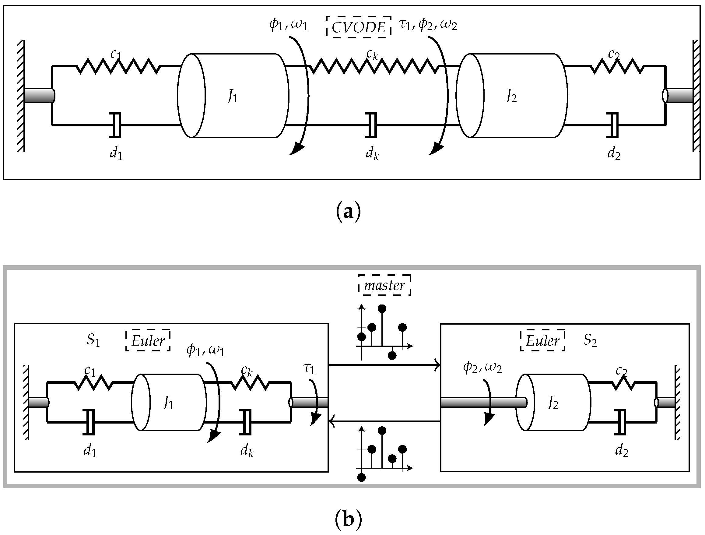
The implementation of the co-simulation slaves (Figure 3b) follows the FMI standard [3]. Since slaves are compiled together with the master, the shared library and the interface description are not packaged together for ease of implementation. Models solved by the slaves are described in the following equations.

The example system consists of two slaves $i\in \{1,2\}$ that solve the following system of equations

$$\begin{array}{cc}\hfill & {\dot{\mathbf{x}}}_i\left(t\right)={\mathbf{f}}_i({\mathbf{x}}_i\left(t\right),{\mathbf{u}}_i\left(t\right))={\mathbf{A}}_i{\mathbf{x}}_1\left(t\right)+{\mathbf{B}}_1{\mathbf{u}}_1\left(t\right),\hfill \end{array}$$

(40a)

$$\begin{array}{cc}\hfill & {\mathbf{y}}_i\left(t\right)={\mathbf{g}}_i({\mathbf{x}}_i\left(t\right),{\mathbf{u}}_i\left(t\right))={\mathbf{C}}_i{\mathbf{x}}_i\left(t\right)+{\mathbf{D}}_i{\mathbf{u}}_i\left(t\right),\hfill \end{array}$$

(40b)

$$\begin{array}{cc}\hfill & {\mathbf{x}}_i\left(0\right)={\mathbf{x}}_{i0}\hfill \end{array}$$

(40c)

connected by

$$\begin{array}{cc}\hfill {\mathbf{u}}_1\left(t\right)={\mathbf{y}}_2\left(t\right),& {\mathbf{u}}_2\left(t\right)={\mathbf{y}}_1\left(t\right)\hfill \end{array}$$

(41)

where

$$\begin{array}{l}{\mathbf{y}}_1\left(t\right)=\left[\begin{array}{c}{\tau }_1\left(t\right)\end{array}\right],{\mathbf{u}}_1\left(t\right)=\left[\begin{array}{c}{\omega }_2\left(t\right)\end{array}\right],\\ {\mathbf{x}}_1\left(t\right)={\left[\begin{array}{ccc}{\varphi }_1\left(t\right)& {\omega }_1\left(t\right)& {\varphi }_2\left(t\right)\end{array}\right]}^T,{\mathbf{x}}_{10}={\left[\begin{array}{ccc}{\varphi }_{10}& {\omega }_{10}& {\varphi }_{20}\end{array}\right]}^T,\\ {\mathbf{A}}_1=\left[\begin{array}{ccc}0& 1& 0\\ -\frac{c_1+c_k}{J_1}& -\frac{d_1+d_k}{J_1}& \frac{c_k}{J_1}\\ 0& 0& 0\end{array}\right],{\mathbf{B}}_1=\left[\begin{array}{c}0\\ \frac{d_k}{J_1}\\ 1\end{array}\right],\\ {\mathbf{C}}_1=\left[\begin{array}{ccc}{c}_k& d_k& -c_k\end{array}\right],{\mathbf{D}}_1=\left[\begin{array}{c}-d_k\end{array}\right]\end{array}$$

(42)

and

$$\begin{array}{l}{\mathbf{y}}_2\left(t\right)=\left[\begin{array}{c}{\omega }_2\left(t\right)\end{array}\right],{\mathbf{u}}_2\left(t\right)=\left[\begin{array}{c}{\tau }_1\left(t\right)\end{array}\right],\\ {\mathbf{x}}_2\left(t\right)={\left[\begin{array}{cc}{\varphi }_2\left(t\right)& {\omega }_2\left(t\right)\end{array}\right]}^T,{\mathbf{x}}_{20}={\left[\begin{array}{cc}{\varphi }_{20}& {\omega }_{20}\end{array}\right]}^T,\\ {\mathbf{A}}_2=\left[\begin{array}{cc}0& 1\\ -\frac{c_2}{J_2}& -\frac{d_2}{J_2}\end{array}\right],{\mathbf{B}}_2=\left[\begin{array}{c}0\\ \frac{1}{J_2}\end{array}\right],\\ {\mathbf{C}}_2=\left[\begin{array}{cc}0& 1\end{array}\right],{\mathbf{D}}_2=\left[\begin{array}{c}0\end{array}\right]\end{array}$$

(43)

Model parameters are set to

$$\begin{array}{l}{J}_1=10\mathrm{kg}{\mathrm{m}}^2,c_1=1\frac{\mathrm{N}\mathrm{m}}{\mathrm{rad}},d_1=1\frac{\mathrm{N}\mathrm{m}\mathrm{s}}{\mathrm{rad}},c_k=1\frac{\mathrm{N}\mathrm{m}}{\mathrm{rad}},\\ d_k=2\frac{\mathrm{N}\mathrm{m}\mathrm{s}}{\mathrm{rad}},{\varphi }_{10}=0.1\mathrm{rad},{\omega }_{10}=0.1\frac{\mathrm{rad}}{\mathrm{s}},J_2=10\mathrm{kg}{\mathrm{m}}^2,\\ c_2=1\frac{\mathrm{N}\mathrm{m}}{\mathrm{rad}},d_2=2\frac{\mathrm{N}\mathrm{m}\mathrm{s}}{\mathrm{rad}},{\varphi }_{20}=0.2\mathrm{rad},{\omega }_{20}=0.1\frac{\mathrm{rad}}{\mathrm{s}}\end{array}$$

(44)

The analytic solution is approximated by a monolithic solution of the system (Figure 3a) solved using the CVODE solver [27] with a tight tolerance bound. The absolute tolerance limit for the solver used is set to ${10}^{-8}$. This solution is used to give a reference solution for the co-simulation and to approximate the numerical error.

The internal equations of co-simulation slaves are solved using the forward Euler method. The forward Euler method is a first-order numerical solver for the same equations

$$\begin{array}{cc}\hfill {\tilde{\mathbf{x}}}_i^{\left(T\left[k-1\right],T\left[k\right]\right]}(t)=& {\tilde{\mathbf{x}}}_i^{\left(T\left[k-2\right],T\left[k-1\right]\right]}\left(T[k-1]\right)\hfill \\ \hfill & +\left(t-T[k-1]\right){\mathbf{f}}_i\left({\tilde{\mathbf{x}}}_i^{\left(T\left[k-2\right],T\left[k-1\right]\right]}\left(T[k-1]\right),{\tilde{\mathbf{u}}}_i^{\left(T\left[k-1\right],T\left[k\right]\right]}\left(T[k-1]\right)\right)\hfill \end{array}$$

(45)

The state derivative values of the Euler solver are equal to

$$\frac{{\mathrm{d}}^n{\tilde{\mathbf{x}}}_i^{\left(T\left[k-1\right],T\left[k\right]\right]}}{{\mathrm{dt}}^n}\left(T\left[k\right]\right)=\left\{\begin{array}{cc}{\mathbf{A}}_i{\tilde{\mathbf{x}}}_i^{\left(T\left[k-2\right],T\left[k-1\right]\right]}\left(T[k-1]\right)+{\mathbf{B}}_i{\tilde{\mathbf{u}}}_i^{\left(T\left[k-1\right],T\left[k\right]\right]}\left(T[k-1]\right),\hfill & n=1\hfill \\ 0,\hfill & n>1\hfill \end{array}\right.$$

(46)

Output polynomials are Taylor polynomials (12) with output derivative values calculated using (18) and

$$\frac{{\mathrm{d}}^n{\tilde{\mathbf{y}}}_i^{\left(T\left[k-1\right],T\left[k\right]\right]}}{{\mathrm{dt}}^n}\left(T\left[k\right]\right)={\mathbf{C}}_i\frac{{\mathrm{d}}^n{\tilde{\mathbf{x}}}_i^{\left(T\left[k-1\right],T\left[k\right]\right]}}{{\mathrm{dt}}^n}\left(T\left[k\right]\right)+{\mathbf{D}}_i\frac{{\mathrm{d}}^n{\tilde{\mathbf{u}}}_i^{\left(T\left[k-1\right],T\left[k\right]\right]}}{{\mathrm{dt}}^n}\left(T\left[k\right]\right),n=1,\dots ,n_i$$

(47)

Input polynomials are Taylor polynomials (14) with input derivative values calculated using (15).

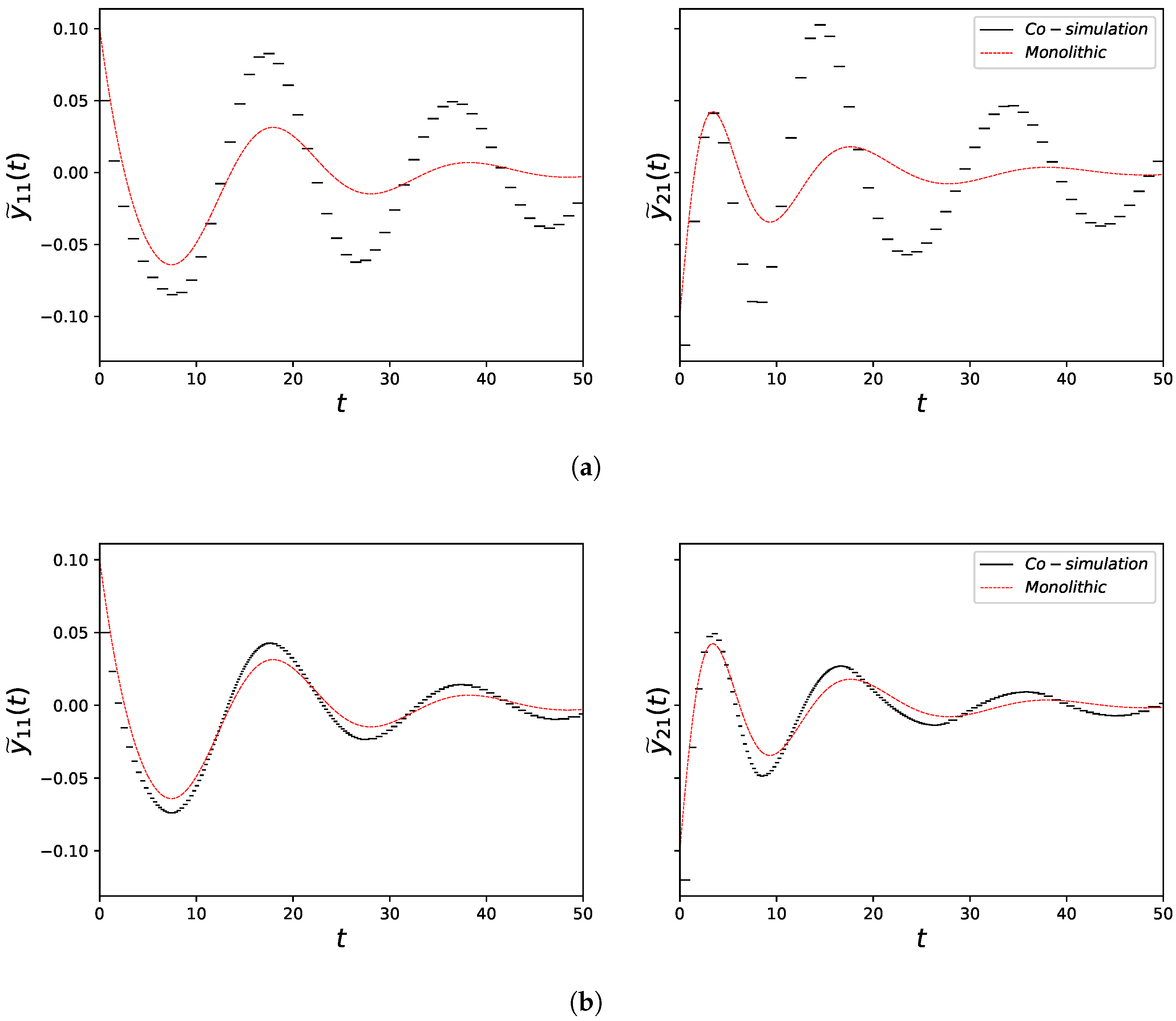
Figure 4a,b shows the piecewise response for both fixed and variable-step co-simulation using Algorithm 1. Figure 4a shows the responses obtained by fixed-step co-simulation with the step size

$$H=H\left[k\right]=H\left[k-1\right]=H_1=1$$

(48)

Figure 4b shows the responses obtained by variable-step co-simulation with the initial step size and tolerance

$$H_1=1,tol=0.005$$

(49)

The step size is controlled by the step controller (39) with the control parameters set to

$$\begin{array}{c}\hfill K_P=0.13,K_I=\frac{1}{15},{\theta }_{max}=2\end{array}$$

(50)

The comparison of figures shows how the step size controller reduces the step size during the co-simulation. In Figure 4a,b

• orders of output (12) and input (14) polynomials are fixed to 0,
• and compared to the monolithic system (Figure 3a) solution found using CVODE (tolerance ${10}^{-8}$, [27]).

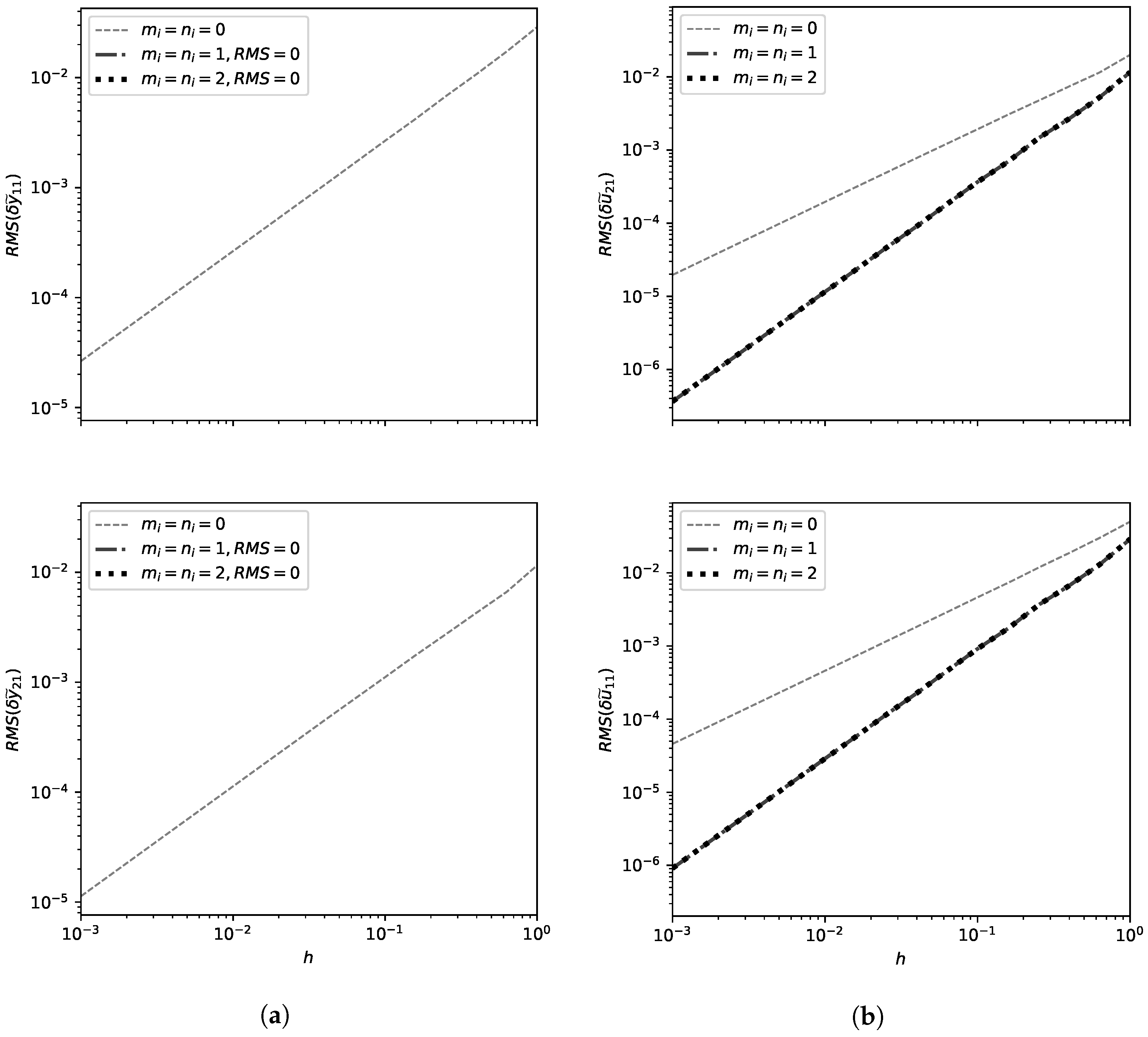
Theorems 2 and 3 show that the connection and the output defect can be limited by reducing the communication step size. In order to verify this statement, the root mean square value of the connection

$$RMS\left(\delta {\tilde{u}}_{i1}\right)=\sum _{0<kH⩽t_{end}}{\int }_{T\left[k-1\right]}^{T\left[k\right]}\delta {\tilde{u}}_{i1}\left(\tau \right)\mathrm{d}\tau$$

(51)

and output defect

$$RMS\left(\delta {\tilde{y}}_{i1}\right)=\sum _{0<kH⩽t_{end}}{\int }_{T\left[k-1\right]}^{T\left[k\right]}\delta {\tilde{y}}_{i1}\left(\tau \right)\mathrm{d}\tau$$

(52)

is calculated for fixed-step co-simulations with different step sizes

$$H=H\left[k\right]=H\left[k-1\right]=H_1\in \{{10}^{-3},{10}^{-2.8},\dots ,{10}^0\}$$

(53)

The results are shown in Figure 5a,b.

The output defect (2b) is estimated using (32). The order of convergence of the output defect is given with Theorem 3. Figure 5a confirms this theorem. It is interesting to observe the output defect of the Euler solver (45) in Figure 5a. From (12), (40b), (45), (46) and (47) it follows that

$${\tilde{y}}_{i1}^{\left(T\left[k-1\right],T\left[k\right]\right]}\left(t\right)=0.5{\tilde{x}}_{i1}^{\left(T\left[k-1\right],T\left[k\right]\right]}\left(t\right),n_i>0$$

(54)

and

$$\delta {\tilde{y}}_{i1}\left(t\right)=0,n_i>0$$

(55)

for the Euler solver. This result agrees with the asymptotic upper limit from Theorem 3. This is interesting because it shows that the output defect for such a solver setup is zero for any output interpolation order greater than 0. However, the numerical error is larger than that of an analytic solver (Figure 6).

Theorem 2 shows that the connection defect converges (by assuming that the output equations are independent of the input signal), but does not show the order of convergence. The input assignment (15) suggests that the input signal depends on the order of the input polynomial as well as the connected output polynomial. However, Figure 5b shows a relationship between connection defects and an internal solver. The connection defect when using the analytic solver seems to correlate with the interpolation order and appears to be $\mathcal{O}\left(H^{min(m_i,n_i)+1}\right)$. In the case of the Euler solver, the connection defect seems to be limited to $\mathcal{O}\left(H^2\right)$. The latter seems to be a consequence of (46).

The focus of future work will be on the investigation of the order of convergence of connection defects. Theorem 2 uses a simplification to avoid the analysis of direct influences of input signals on output signals. This simplification prevents the analysis of algebraic loops, which could make the system unstable. Direct influences of input signals on output signals have an effect on the local co-simulation error shown in [24]. This indicates that a direct output input dependency could affect the order of the connection defect. This will be a topic for future work, along with the analysis of the influence of the solver on connection defects.

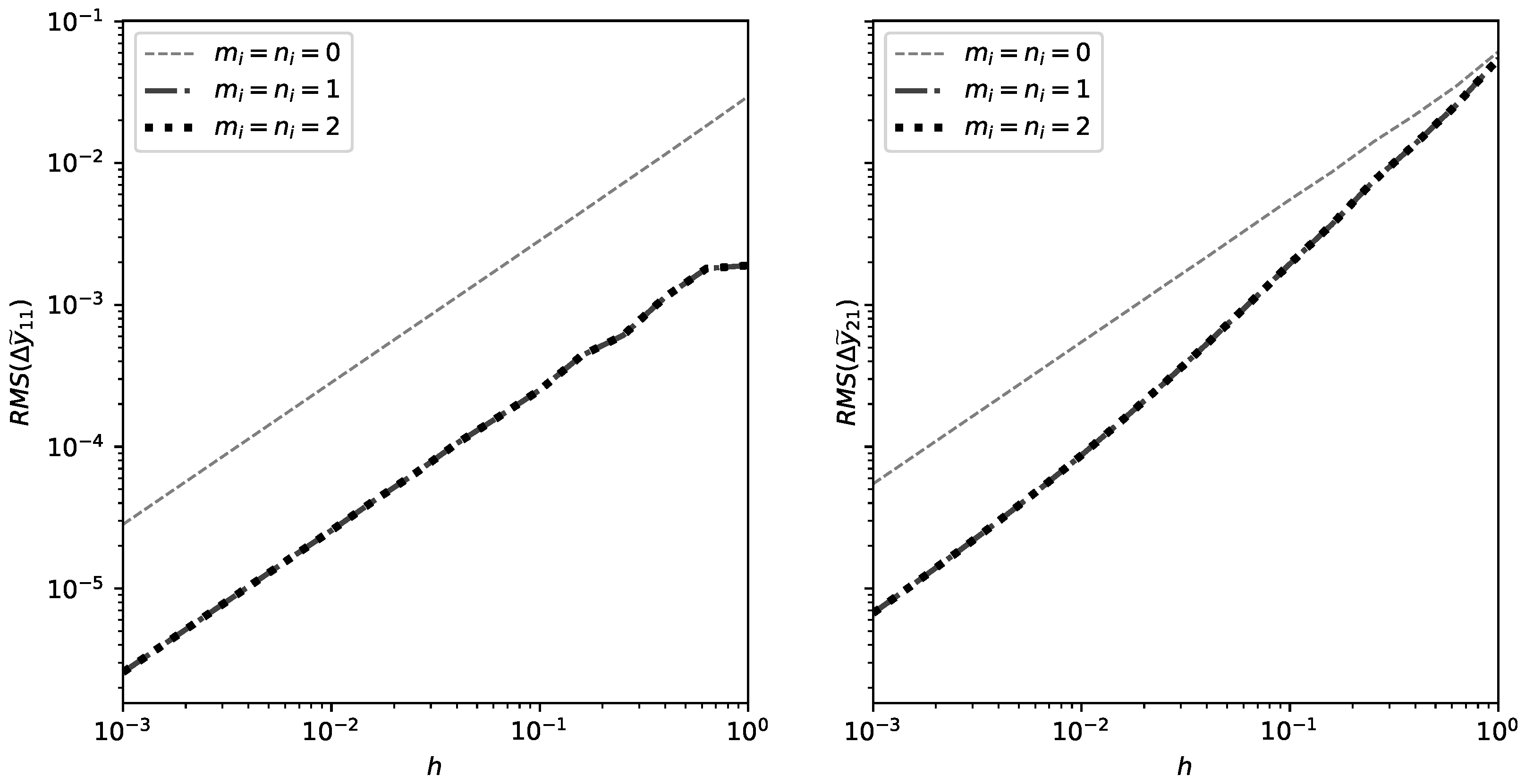
Theorem 1 suggests that by limiting the overall co-simulation defect, the global co-simulation error should be limited. Theorems 2 and 3 show that by limiting the step size, connection and output defects can be limited. Figure 5 confirms this. The three theorems suggest that by limiting the step size, the global co-simulation error can be limited. This is confirmed by Figure 6. It is worth noting that the conclusions given apply to a coupled ordinary differential system 1.

Reducing the step size limit is not the only way to reduce connection and output defects. The order of the polynomials used to transmit input and output signals also has an effect. This effect can be observed in Figure 6. Theorem 1 shows that the co-simulation error is bounded by connection, output, and integration defects. If defects are

$$\delta \tilde{\mathbf{u}}\left(t\right)=\mathcal{O}\left(H^{p_i}\right),\delta \tilde{\mathbf{y}}\left(t\right)=\mathcal{O}\left(H^{q_i}\right),\delta \tilde{\mathbf{x}}\left(t\right)=\mathcal{O}\left(H^{r_i}\right)$$

(56)

then the errors are

$$\Delta \tilde{\mathbf{u}}\left(t\right)=\mathcal{O}\left(H^{min(p_i,q_i,r_i+1)}\right),\Delta \tilde{\mathbf{y}}\left(t\right)=\mathcal{O}\left(H^{min(p_i,q_i,r_i+1)}\right),\Delta \tilde{\mathbf{x}}\left(t\right)=\mathcal{O}\left(H^{min(p_i,q_i,r_i+1)}\right)$$

(57)

All co-simulation errors are limited by the worst co-simulation defect. Figure 6 shows how the integration defect of the Euler solver limits the co-simulation error to $\mathcal{O}\left(H\right)$.

Co-simulation errors can be limited by limiting the co-simulation defects. The rate of convergence of the output defect is given by Theorem 3. It is important to note that the order of convergence for the output defect estimate is influenced by the Euler solver. The Euler solver brakes the assumption (33). This is an example where an integration defect can affect the output error estimate.

It is interesting to observe the effect of the internal solver on the connection defect. In Figure 5b, it can be seen that for the Euler solver and larger orders of extrapolation for input and output signals the connection defect is $\mathcal{O}\left(H\right)$. The connection defect (17) in the explicit co-simulation is influenced by the difference of the state signal at different co-simulation steps (26). This observation suggests that a connection defect can be used to detect numerical errors introduced by solving state, output, and connection equations. The authors plan future work to rigorously analyze whether there are conditions under which this hypothesis is true.

The previous experiments use fixed-step co-simulation to confirm Theorems 1, 2 and 3. Theorem 1 shows that defect control can be used to limit the co-simulation error. Theorems 2 and 3 show that output and connection defects can be limited by limiting the step size. The previous experiments and theorems justify the use of variable step size co-simulation using defect control. The next experiments show the results of applying the variable-step Jacobi co-simulation method to the system (40) and (41). The method is presented in Algorithm 1 and the step size is calculated with (39). The numerical experiment was performed with the reference $tol=0.1$, controller parameters (50) and the initial step size $H_1=0.001$. The comparison of the obtained output signals with the monolithic solution (Figure 3a) is shown in Figure 4b.

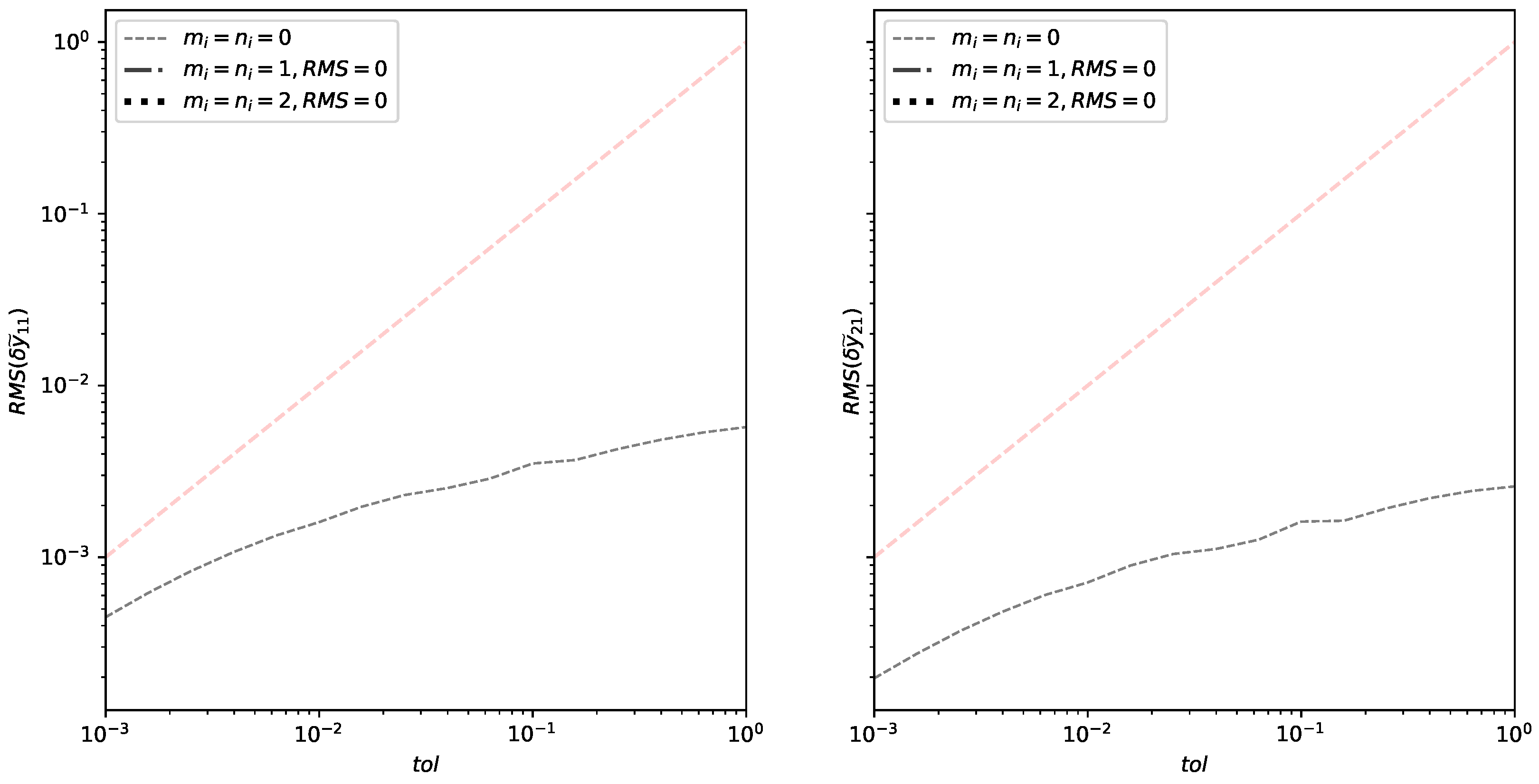
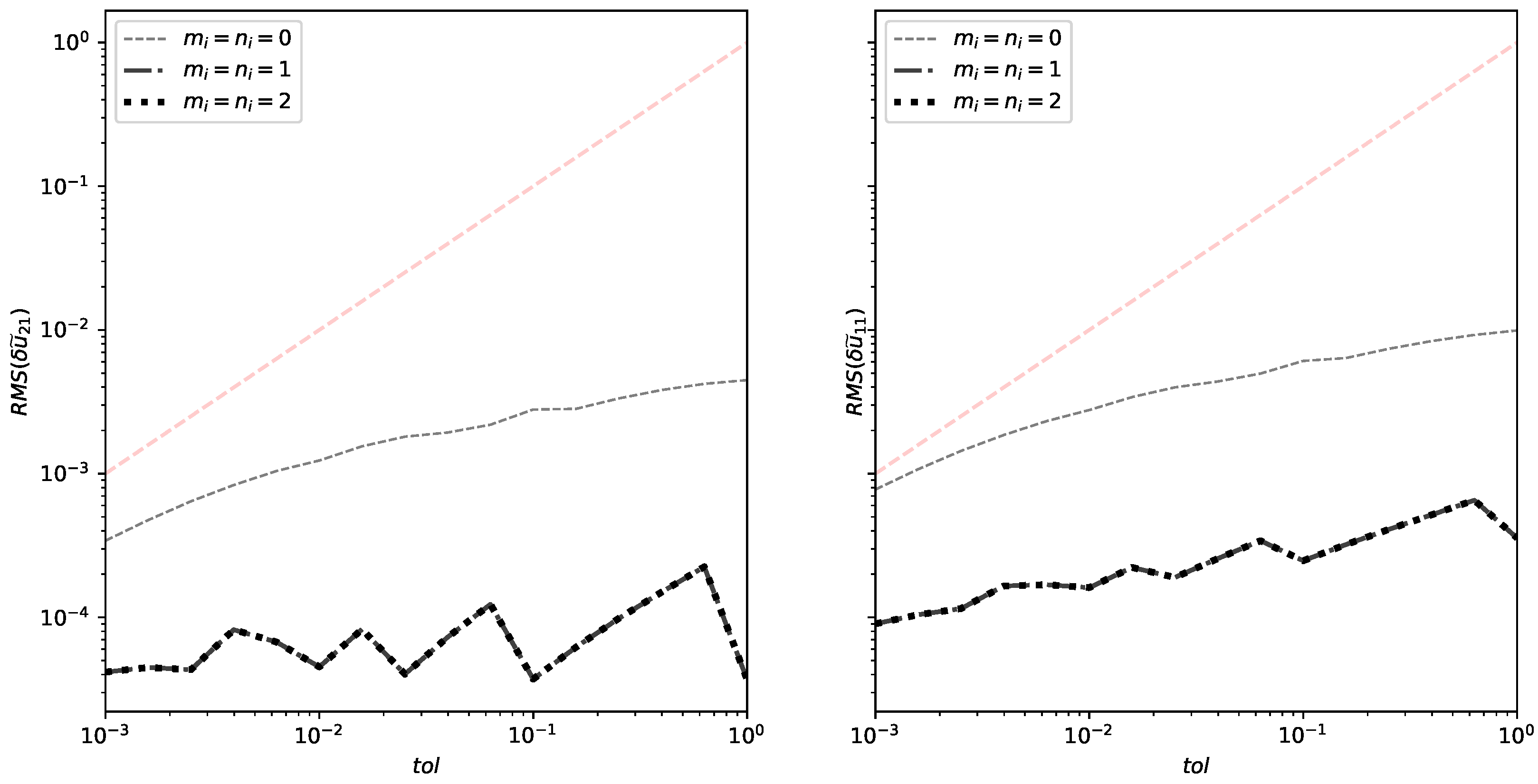
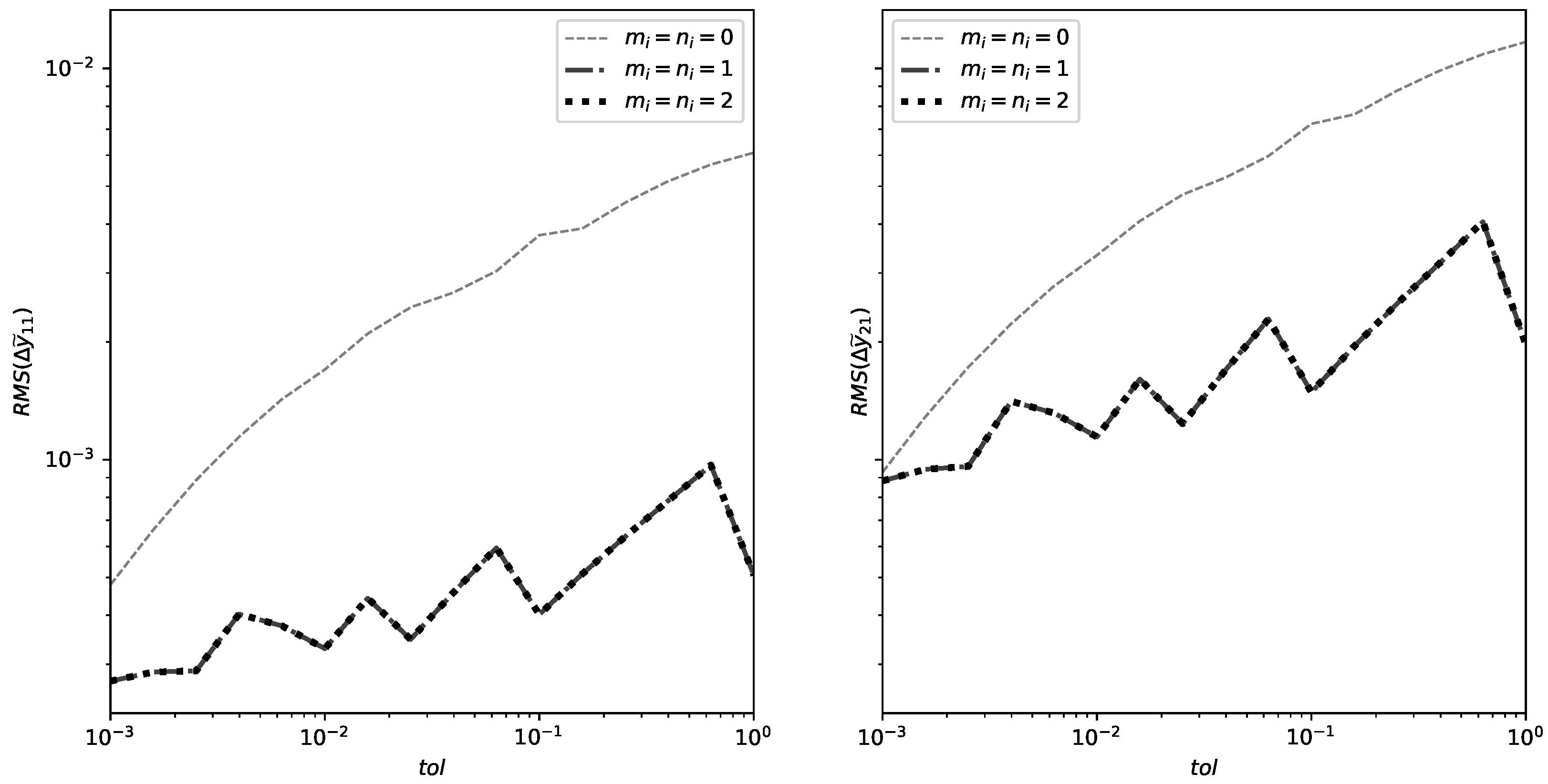
Next, the tolerance was varied

$$tol\in \{{10}^{-3},{10}^{-2.8},\dots ,{10}^0\}$$

(58)

to demonstrate that such a controller can limit output and connection defects. Figure 7 shows that the output defect is limited by the tolerance. Figure 8 shows that the connection defect is limited by the tolerance. This may not always be the case for explicit co-simulation. In the presented experiments, the initial step size was set to small $H_1=0.001$ to ensure that the numerical defect produced in the initial step stays within tolerance. The experiment shows that by controlling (38) both connection and output defects can be controlled.

Furthermore, Figure 9 shows that by reducing the tolerance, the co-simulation error can be reduced. It is interesting to observe that plots of the output defect (Figure 7) and connection defect (Figure 8) are similar shapes to the error plot (Figure 9). This comparison suggests that there are cases where such variable step co-simulation can be used successfully.

It should be noted that the integration defect (2a) is not directly controlled in this example. In the case of the analytic solver, the defect is completely eliminated. In the case of the Euler solver (45), the integration defect is $\mathcal{O}\left(H\right)$. In practice, co-simulation slaves are black boxes without the ability to monitor the integration. This is why the integration defect is not included in this analysis.

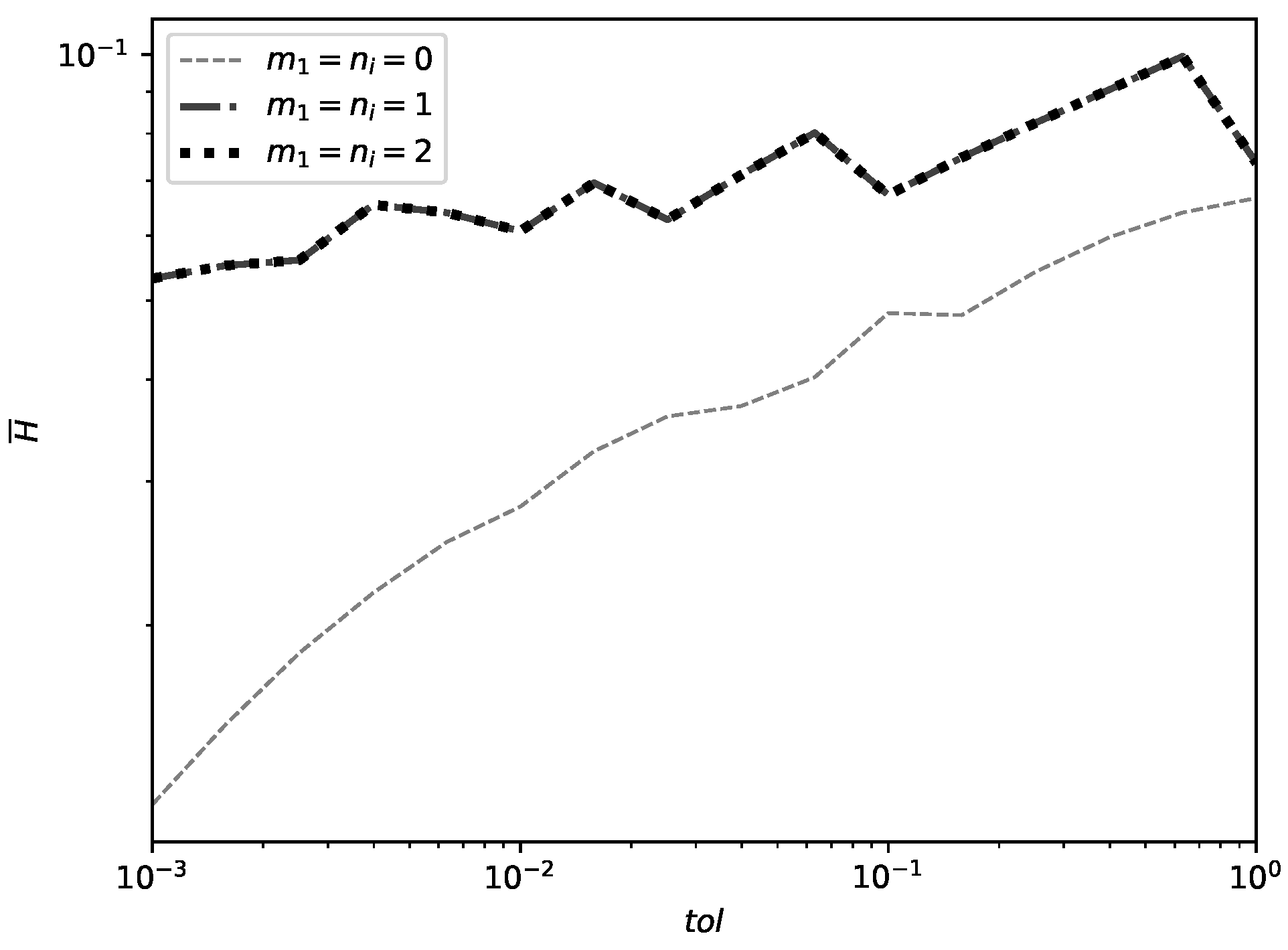
In Figure 9, it can be seen that co-simulation errors are similar in order of magnitude for different extrapolation orders. Figure 10 shows the benefit of increasing the extrapolation order. It shows how an average step size during co-simulation depends on the requested tolerance. The step size controller takes smaller steps to achieve the same tolerance if higher extrapolation order is used. This conclusion may not be generalized to more complex subsystems. It shows the idea that an extrapolation order could be used to decrease the CPU and communication network load during co-simulation.

5. Conclusions and Future Work

This article presents an analysis of the co-simulation defect for a system of coupled ordinary differential equations. The analysis is motivated to deepen the understanding of the co-simulation configuration. In practice, co-simulation slaves are black boxes coupled with connection equations (Figure 1). A quality measure that does not require knowledge of the slave’s internal equations can facilitate the co-simulation configuration. The defect analysis was only applied to the co-simulation in [15]. This article continues the application of defect analysis and applies it to variable-step co-simulation with different orders of interpolation polynomials.

The main contribution of this article is a non-iterative co-simulation method with variable communication step size (Figure 2, Algorithm 1). Theorem 1 states that the co-simulation error is bounded if the co-simulation defect is bounded. Theorem 2 and Theorem 3 show that the connection and the output defect can be limited by reducing the communication step size. These theorems justify the use of variable step co-simulation based on defect control. Section 4 shows an application of the proposed method to an example of a two-mass oscillator and gives a verification of the above statements.

Such a method is valuable in practice because it requires little configuration. The parameters for the procedure are the initial communication step size $H_1$ and the required tolerance $tol$. The method does not require a co-simulation slave to repeat a communication step. This relaxes the implementation requirements for co-simulation slaves. In addition, like any variable step method, it can save computation time by calculating the step size for the results of the desired quality.

One goal of future work would be to see if there is a way to eliminate the need to perform additional sampling of the communication points to estimate output defects. It is worth considering under what conditions the calculations of the connection defect are sufficient to assess the quality of the co-simulation.

Another goal of future work would be to focus on the properties of a model and try to estimate the correct initial step size $H_1$ for co-simulation. This would reduce the configuration effort even further and achieve an almost ideal configuration. In this case, only the required quality of the co-simulation is requested by a user $tol$.

References

- Kübler, R.; Schiehlen, W. Two Methods of Simulator Coupling. Math. Comput. Model. Dyn. Syst. 2000, 6, 93–113. [Google Scholar] [CrossRef]
- Gomes, C.; Thule, C.; Broman, D.; Larsen, P.G.; Vangheluwe, H. Co-Simulation: A Survey. ACM Comput. Surv. 2018, 51, 49:1–49:33. [Google Scholar] [CrossRef]
- Functional Mock-Up Interface for Model Exchange and Co-Simulation, Version 2.0. 2014. Available online: https://svn.modelica.org/fmi/branches/public/specifications/v2.0/FMI_for_ModelExchange_and_CoSimulation_v2.0.pdf (accessed on 26 October 2018).
- Blochwitz, T.; Otter, M.; Akesson, J.; Arnold, M.; Clauss, C.; Elmqvist, H.; Friedrich, M.; Junghanns, A.; Mauss, J.; Neumerkel, D.; et al. Functional mockup interface 2.0: The standard for tool independent exchange of simulation models. In Proceedings of the 9th International MODELICA Conference, Munich, Germany, 3–5 September 2012; Linköping University Electronic Press: Linköping, Sweden, 2012; pp. 173–184. [Google Scholar] [CrossRef] [Green Version]
- Tools | Functional Mock-Up Interface. Available online: https://fmi-standard.org/tools/ (accessed on 1 May 2021).
- Schweizer, B.; Li, P.; Lu, D. Explicit and implicit cosimulation methods: Stability and convergence analysis for different solver coupling approaches. J. Comput. Nonlinear Dyn. 2015, 10, 051007. [Google Scholar] [CrossRef]
- Hairer, E.; Nørsett, S.P.; Wanner, G. Solving Ordinary Differential Equations. 1, Nonstiff Problems; Springer: Berlin/Heidelberg, Germany, 1991. [Google Scholar]
- Isermann, R.; Schaffnit, J.; Sinsel, S. Hardware-in-the-loop simulation for the design and testing of engine-control systems. Control. Eng. Pract. 1999, 7, 643–653. [Google Scholar] [CrossRef]
- Fathy, H.K.; Filipi, Z.S.; Hagena, J.; Stein, J.L. Review of hardware-in-the-loop simulation and its prospects in the automotive area. In Proceedings of the Modeling and Simulation for Military Applications. International Society for Optics and Photonics, Kissimmee, FL, USA, 18–21 April 2006; Volume 6228, p. 62280E. [Google Scholar] [CrossRef]
- Glumac, S.; Varga, N.; Raos, F.; Kovačić, Z. Co-simulation perspective on evaluating the simulation with the engine test bench in the loop. Automatika 2022, 63, 275–287. [Google Scholar] [CrossRef]
- Borutzky, W. Bond Graph Modelling of Engineering Systems; Springer: Berlin/Heidelberg, Germany, 2011; Volume 103. [Google Scholar]
- Siciliano, B.; Khatib, O.; Kröger, T. Springer Handbook of Robotics; Springer: Berlin/Heidelberg, Germany, 2008; Volume 200. [Google Scholar]
- Shampine, L.F. Error estimation and control for ODEs. J. Sci. Comput. 2005, 25, 3–16. [Google Scholar] [CrossRef]
- Arnold, M.; Clauß, C.; Schierz, T. Error analysis and error estimates for co-simulation in FMI for model exchange and co-simulation V2.0. In Progress in Differential-Algebraic Equations; Springer: Berlin/Heidelberg, Germany, 2014; pp. 107–125. [Google Scholar]
- Glumac, S. Automated Configuring of Non-Iterative Co-Simulation Modeled by Synchronous Data Flow. Ph.D. Thesis, Faculty of Electrical Engineering and Computing, University of Zagreb, Zagreb, Croatia, 2022. [Google Scholar]
- Enright, W. Continuous numerical methods for ODEs with defect control. J. Comput. Appl. Math. 2000, 125, 159–170. [Google Scholar] [CrossRef] [Green Version]
- Shampine, L.F. Solving ODEs and DDEs with residual control. Appl. Numer. Math. 2005, 52, 113–127. [Google Scholar] [CrossRef]
- Gustafsson, K.; Lundh, M.; Söderlind, G. A PI stepsize control for the numerical solution of ordinary differential equations. BIT Numer. Math. 1988, 28, 270–287. [Google Scholar] [CrossRef]
- Nguyen, P.H. Interpolation and Error Control Schemes for Algebraic Differential Equations Using Continuous Implicit Runge-Kutta Methods; Department of Computer Science, University of Toronto: Toronto, ON, USA, 1995. [Google Scholar]
- Spitzbart, A. A Generalization of Hermite’s Interpolation Formula. Am. Math. Mon. 1960, 67, 42–46. [Google Scholar] [CrossRef]
- Busch, M.; Schweizer, B. An explicit approach for controlling the macro-step size of co-simulation methods. In Proceedings of the 7th European Nonlinear Dynamics Conference (ENOC 2011), Rome, Italy, 24–29 July 2011; pp. 1–6. [Google Scholar]
- Benedikt, M.; Watzenig, D.; Hofer, A. Modelling and analysis of the non-iterative coupling process for co-simulation. Math. Comput. Model. Dyn. Syst. 2013, 19, 451–470. [Google Scholar] [CrossRef]
- Schweizer, B.; Lu, D. Predictor/corrector co-simulation approaches for solver coupling with algebraic constraints. ZAMM J. Appl. Math. Mech. Z. Für Angew. Math. Und Mech. 2015, 95, 911–938. [Google Scholar] [CrossRef]
- Busch, M. Continuous approximation techniques for co-simulation methods: Analysis of numerical stability and local error. ZAMM J. Appl. Math. Mech. 2016, 96, 1061–1081. [Google Scholar] [CrossRef]
- Glumac, S.; Kovacic, Z. Relative consistency and robust stability measures for sequential co-simulation. In Proceedings of the 13th International Modelica Conference, Regensburg, Germany, 4–6 March 2019; Linköping University Electronic Press: Linköping, Sweden, 2019; p. 157. [Google Scholar] [CrossRef]
- Sglumac/DefectAnalysisArticle. 2023. Available online: https://github.com/sglumac/DefectAnalysisArticle (accessed on 25 February 2023).
- Hindmarsh, A.C.; Brown, P.N.; Grant, K.E.; Lee, S.L.; Serban, R.; Shumaker, D.E.; Woodward, C.S. SUNDIALS: Suite of nonlinear and differential/algebraic equation solvers. ACM Trans. Math. Softw. (TOMS) 2005, 31, 363–396. [Google Scholar] [CrossRef]
Figure 1.
The underlying model for the analysis in this article is coupled ordinary differential equations [15]. Co-simulation slave equations are colored gray because they are not available to the master. Output equations are lighter colored because this article suggests that the master should estimate the output defect.
Figure 2.
This article uses a non-iterative variant of the Jacobi co-simulation method with variable steps to demonstrate co-simulation defect control.
Figure 3.
During co-simulation, a co-simulation master orchestrates co-simulation slaves. In the case of the monolithic simulation, a solver solves the entire system of equations: (a) Monolithic simulation; (b) Co-simulation.
Figure 4.
The diagrams show numerical solutions that were calculated with the Jacobi co-simulation method (Algorithm 1). The numerical solutions are compared with the monolithic solution: (a) Fixed step; (b) Variable step.
Figure 5.
The diagrams show the defects of the fixed-step Jacobi co-simulation method (Algorithm 1, ) and different orders of interpolation polynomials : (a) Output defects; (b) Connection defects.
Figure 6.
The diagrams show the numerical errors of the fixed-step Jacobi co-simulation method (Algorithm 1, ), different orders of interpolation polynomials and different internal subsystem solvers.
Figure 7.
The diagrams show the output defects of the variable-step Jacobi co-simulation method (Algorithm 1, (39) and (50), ) and different orders of interpolation polynomials.
Figure 8.
The diagrams show the connection defects of the variable-step Jacobi co-simulation method (Algorithm 1, (39) and (50), ), different orders of interpolation polynomials and different internal subsystem solvers.
Figure 9.
The diagrams show the numerical errors of the variable-step Jacobi co-simulation method (Algorithm 1, (39) and (50), ), different orders of interpolation polynomials and different internal subsystem solvers.
Figure 10.
The diagrams show the average step sizes of the variable-step Jacobi co-simulation method (Algorithm 1, (39) and (50), ), different orders of interpolation polynomials and different internal subsystem solvers.
Disclaimer/Publisher’s Note: The statements, opinions and data contained in all publications are solely those of the individual author(s) and contributor(s) and not of MDPI and/or the editor(s). MDPI and/or the editor(s) disclaim responsibility for any injury to people or property resulting from any ideas, methods, instructions or products referred to in the content. |
© 2023 by the authors. Licensee MDPI, Basel, Switzerland. This article is an open access article distributed under the terms and conditions of the Creative Commons Attribution (CC BY) license (https://creativecommons.org/licenses/by/4.0/).
Share and Cite
MDPI and ACS Style
Glumac, S.; Kovačić, Z. Defect Analysis of a Non-Iterative Co-Simulation. Mathematics 2023, 11, 1342. https://doi.org/10.3390/math11061342
AMA Style
Glumac S, Kovačić Z. Defect Analysis of a Non-Iterative Co-Simulation. Mathematics. 2023; 11(6):1342. https://doi.org/10.3390/math11061342
Chicago/Turabian StyleGlumac, Slaven, and Zdenko Kovačić. 2023. "Defect Analysis of a Non-Iterative Co-Simulation" Mathematics 11, no. 6: 1342. https://doi.org/10.3390/math11061342
Note that from the first issue of 2016, this journal uses article numbers instead of page numbers. See further details here.