On a Method for Optimizing Controlled Polynomial Systems with Constraints

Abstract

A new optimization approach is considered in the class of polynomial in-state optimal control problems with constraints based on nonlocal control improvement conditions, which are constructed in the form of special fixed-point problems in the control space. The proposed method of successive approximations of control retains all constraints at each iteration and does not use the operation of parametric variation of control at each iteration, in contrast to known gradient methods. In addition, the initial approximation of the iterative process may not satisfy the constraints, which is a significant factor in increasing the efficiency of the approach. The comparative efficiency of the proposed method of fixed points in the considered class of problems is illustrated in a model example.

1. Introduction

Polynomial optimal control problems arise in many topical applications. First, state-polynomial systems of ordinary differential equations are traditionally used to describe models of ecological-economic [1,2,3], biological [4,5,6] processes, including models of immunological processes with delays [7]. It should be noted that, in general, questions about the adequacy of the introduction of controls and the choice of optimization criteria when setting the corresponding optimal control problems, in particular, biomedical and ecological-economic processes, still need further research. The state of affairs here is such that the apparatus of optimal control methods at the present stage acts as a means of studying models, showing their consistency and adequacy to real processes, testing hypotheses, and solving controllability problems, i.e., transferring a process from one state to another. Second, various classes of polynomial optimal control problems can be formed by regularizing inverse problems of mathematical physics. In particular, in problems of identification of parameters of systems of ordinary differential equations [8,9]. Third, polynomial optimal control problems can be formed for polynomial approximation of the right parts of controlled nonlinear systems for their approximate solution [10].

Polynomial systems of ordinary differential equations are also considered in the problems of observability, controllability, stabilization, and regulation of controlled systems [11,12,13,14,15]. Actual problems of the analysis of polynomial systems are the issues of stability and qualitative analysis of solutions to systems [16,17,18,19,20]. To solve polynomial systems of differential equations, special approaches and methods are being developed [21,22].

In connection with the above, it seems relevant to develop specialized mathematical and algorithmic support for the effective solution of classes of polynomial optimal control problems. This software can serve as a tool for automating research and be the basis for mobile expert automated decision-making systems with intelligent support that do not require time-consuming experimental tuning of optimization methods for a specific task of the class under consideration.

A well-known approach to solving some classes of polynomial optimal control problems is methods of partial discretization with respect to controlled variables with a reduction to problems of finite-dimensional quadratic programming [23,24]. Another specialized approach focuses on the class of controllable linear in-state systems with a quadratic optimality criterion without constraints, for which nonlocal control improvement methods were proposed in [25]. These methods are based on special formulas for the increment of the objective functional that do not contain residual expansion terms. Control improvement is achieved as a result of solving two Cauchy problems. This feature of the methods is an essential factor for improving the efficiency of solving optimal control problems, which is estimated by the total number of solved Cauchy problems. Another new approach was developed for polynomial in state optimal control problems without constraints, for which nonlocal control improvement methods generalizing the methods of [25] were constructed in [26,27]. These methods are also based on non-standard increment formulas of the objective functional without residual expansion terms, for which special modifications of the standard conjugate system were developed. Improvement of control is achieved as a result of solving a boundary value problem, which is much simpler than the known boundary value problem of the maximum principle. In the class of optimal control problems linear in state, the solution of such a boundary value problem is reduced to solving two Cauchy problems, and the considered methods become equivalent to the methods of [25]. In the general polynomial case, to solve the above boundary value problem for improving control, iterative algorithms were developed based on the well-known perturbation method in mathematics.

In this paper, in the considered class of polynomial optimal control problems with constraints, we construct conditions for improving control with the form of a special fixed-point problem in the control space. To solve problems of the class under consideration, iterative algorithms are proposed based on the well-known theory and methods of fixed points.

2. Polynomial Optimal Control Problem

We consider a class of polynomial in-state and linear in-control problems of optimal control with one terminal constraint:

$$\dot{x}\left(t\right)=A(x\left(t\right),t)u\left(t\right)+b(x\left(t\right),t),x\left(t_0\right)=x^0,u\left(t\right)\in U,t\in T=[t_0,t_1],$$

(1)

$${\Phi }_0\left(u\right)=\langle c,x\left(t_1\right)\rangle \to \underset{u\in V}{inf},$$

(2)

$${\Phi }_1\left(u\right)=x_1\left(t_1\right)-x_1^1=0,$$

(3)

where $x=(x_1\left(t\right),x_2\left(t\right),\dots x_n\left(t\right))$ is the state vector, $u=(u_1\left(t\right),u_2\left(t\right),\dots u_r\left(t\right))$ is the control vector. The interval T is fixed. The initial state $x^0\in R^n$, the value $x_1^1\in R$, the vector $c=(c_1,c_2,\dots ,c_n)$ are given, while $c_1=0$. The matrix function $A(x,t)$ and the vector function $b(x,t)$ are polynomial in x of degree $l\ge 1$ and continuous in t on the set $R^n\times T$. The set of control values $U\subset R^r$ is compact and convex. The set of available controls V is considered in the space of piecewise continuous functions $PC\left(T\right)$ on the interval T:

$$V=\left\{u\in PC\left(T\right):u\left(t\right)\in U,t\in T\right\}.$$

For the scalar product of vectors, the standard notation $\langle ·,·\rangle$ is used.

Under the considered conditions for setting the problem (1)–(3), the local existence of a unique solution to the Cauchy problem (1) is guaranteed for any available control. The global existence of a solution to the Cauchy problem (1) over the entire considered time interval is assumed by default. Sufficient conditions for the existence of a global solution for nonlinear Cauchy problems are known in the literature. In particular, such conditions are given in [25].

For available control $v\in V$ we denote by $x(t,v),t\in T$ the solution of the Cauchy problem (1) for $u\left(t\right)=v\left(t\right)$, $t\in T$. Denote the set of admissible controls:

$$W=\left\{u\in V:x_1(t_1,u)=x_1^1\right\}.$$

Many polynomial optimal control problems with phase, terminal, and mixed constraints can be reduced to the form (1)–(3) using standard methods of penalizing for violation of constraints. In particular, the general polynomial in state and linear in control optimal control problem with functional equality constraints, in which the functionals specifying the goal and constraints are, respectively, of the form:

$${\Phi }_0\left(u\right)\to inf,{\Phi }_i\left(u\right)=0,i=1,\dots ,s,s\ge 1,$$

$${\Phi }_i\left(u\right)={\phi }_i\left(x\left(t_1\right)\right)+{\int }_T(d_i(x\left(t\right),t)+\langle g_i(x\left(t\right),t),u\rangle )dt,i=0,\dots ,s.$$

In this problem, the functions ${\phi }_i\left(x\right)$, $i=0,\dots ,s$ are polynomials of degree $l_1\ge 1$ on $R^n$, the functions $d_i(x,t)$, $g_i(x,t)$, $i=0,\dots ,s$ are polynomial in x of degree $l_1\ge 1$ and continuous in t on $R^n\times T$.

For problem (1)–(3), the Pontryagin function has the form:

$$H(p,x,u,t)=H_0(p,x,t)+\langle H_1(p,x,t),u\rangle ,$$

where $p\in R^n$ is the conjugate vector, $H_0(p,x,t)=\langle p,b(x,t)\rangle$, $H_1(p,x,t)=A{(x,t)}^{T}p$.

We introduce the regular Lagrange functional with the multiplier $\lambda \in R$:

$$L(u,\lambda )={\Phi }_0\left(u\right)+\lambda {\Phi }_1\left(u\right)=\langle c,x\left(t_1\right)\rangle +\lambda (x_1\left(t_1\right)-x_1^1).$$

Let us consider an auxiliary problem of optimal control without constraints:

$$L(u,\lambda )\to \underset{u\in V}{inf}.$$

(4)

In accordance with [26,27] for controls $u^0\in V$, $v\in V$, there is a formula for the increment of the Lagrange functional without remainder terms of the expansions:

$${\Delta }_{v}L(u^0,\lambda )=L(v,\lambda )-L(u^0,\lambda )=-{\int }_T\langle H_1(p(t,u^0,v,\lambda ),x(t,v),t),v\left(t\right)-u^0\left(t\right)\rangle dt.$$

(5)

In Formula (5), the function $p(t,u^0,v,\lambda ),t\in T$ is the solution of the modified conjugate system:

$$\begin{array}{c}\dot{p}\left(t\right)=-H_x-\frac{1}{2!}{\langle H_x,z\rangle }_x-\dots -\frac{1}{l!}{\langle \dots {\langle {\langle H_x,z\rangle }_x,z\rangle }_x\dots ,z\rangle }_x,\\ \\ p_1\left(t_1\right)=-\lambda ,p_i\left(t_1\right)=-c_i,i=\overline{2,n},\end{array}$$

(6)

in which the partial derivatives with respect to x are calculated with the values of the arguments $x=x(t,u^0)$, $u=u^0\left(t\right)$, $z=x(t,v)-x(t,u^0)$. For the partial derivatives of the Pontryagin function with respect to x and u, the corresponding standard notation $H_x$ and $H_u$ is used.

In a problem linear in state and control, the modified conjugate system (6) becomes equivalent to the standard conjugate system:

$$\dot{\psi }\left(t\right)=-H_x,{\psi }_1\left(t_1\right)=-\lambda ,{\psi }_i\left(t_1\right)=-c_i,i=\overline{2,n}.$$

(7)

Let $\psi (t,u^0,\lambda )$, $t\in T$ be the solution of the Cauchy problem (7) for $x=x(t,u^0)$, $u=u^0\left(t\right)$. It’s obvious that $p(t,u^0,u^0,\lambda )=\psi (t,u^0,\lambda )$, $t\in T$.

3. Conditions and Method for Improving Control

For the control $u^0\in V$ and the given parameter $\alpha >0$, consider the auxiliary vector function:

$$u^{\alpha }(p,x,t)=P_U\left(u^0\left(t\right)+\alpha H_1(p,x,t)\right),p\in R^n,x\in R^n,t\in T,$$

where $P_U$ is the projection operator onto a set U in the Euclidean norm.

We will assume that the problem of projection onto the set U admits an analytical solution.

In accordance with the well-known property of the projection operator, we have the inequality:

$${\int }_T\langle H_1(p,x,t),u^{\alpha }(p,x,t)-u^0\left(t\right)\rangle dt\ge \frac{1}{\alpha }{\int }_T\left|\right|u^{\alpha }(p,x,t)-u^0\left(t\right){\left|\right|}^{2}dt.$$

(8)

For the Euclidean norm of a vector, the standard notation $\left|\right|·\left|\right|$ is used.

For the auxiliary problem (4), the known necessary optimality condition (Pontryagin’s maximum principle) for control $u\in V$ using a function $u^{\alpha }$ can be represented in the following form:

$$u\left(t\right)=u^{\alpha }(\psi (t,u,\lambda ),x(t,u),t),t\in T.$$

This condition is equivalent to the well-known condition of the maximum principle in the non-degenerate problem (1)–(3) for control $u\in W$ with a certain multiplier $\lambda \in R$. Controls that satisfy the condition of the maximum principle are called extremal controls for convenience.

Let the control $v\in V$ be a solution of the following system of equations:

$$\begin{array}{c}v\left(t\right)=u^{\alpha }(p(t,u^0,v,\lambda ),x(t,v),t),t\in T,\lambda \in R,\\ {\Phi }_1\left(v\right)=x_1(t_1,v)-x_1^1=0.\end{array}$$

(9)

It is obvious that $v\in W$. From inequality (8) and the increment formula (5), we obtain an estimate for the increment of the Lagrange functional:

$${\Delta }_{v}L(u^0,\lambda )\le -\frac{1}{\alpha }{\int }_T\left|\right|v\left(t\right)-u^0\left(t\right){\left|\right|}^{2}dt.$$

(10)

If $u^0\in W$, then on the controls $u^0,v$, the Lagrange functional coincides with the objective functional. Then, by virtue of estimate (10), there is an improvement in the objective functional ${\Phi }_0$ with the estimate:

$${\Delta }_v{\Phi }_0\left(u^0\right)={\Phi }_0\left(v\right)-{\Phi }_0\left(u^0\right)\le -\frac{1}{\alpha }{\int }_T\left|\right|v\left(t\right)-u^0\left(t\right){\left|\right|}^{2}dt.$$

(11)

For extremal control $u^0\in W$ in non-degenerate problem (1)–(3), system (9) has an obvious solution $v=u^0$. Thus, if system (9) for an extremal control $u^0\in W$ has a non-unique solution, then the extremal control $u^0\in W$ can be rigorously improved with estimate (11).

Based on these properties, we obtain the following assertions.

Theorem 1

(maximum principle). Let the control $u^0\in W$ be optimal in the non-degenerate problem (1)–(3). Then $u^0\in W$ is a solution to system (9) for some $\alpha >0$.

Theorem 2

(strengthened necessary optimality condition). Let the control $u^0\in W$ be optimal in the non-degenerate problem (1)–(3). Then for all $\alpha >0$, the control $u^0\in W$ is the only solution to system (9).

Thus, system (9) allows us to formulate a new necessary optimality condition in the non-degenerate problem (1)–(3), strengthened in comparison with the well-known maximum principle.

Theorem 3.

System (9) is equivalent to the following boundary value problem:

$$\begin{array}{c}\dot{x}\left(t\right)=A(x\left(t\right),t)u^{\alpha }(p\left(t\right),x\left(t\right),t)+b(x\left(t\right),t),x\left(t_0\right)=x^0,x_1\left(t_1\right)=x_1^1,\\ \dot{p}\left(t\right)=-H_x-\frac{1}{2!}{\langle H_x,z\rangle }_x-\dots -\frac{1}{l!}{\langle \dots {\langle {\langle H_x,z\rangle }_x,z\rangle }_x\dots ,z\rangle }_x,\\ p_1\left(t_1\right)=-\lambda ,p_i\left(t_1\right)=-c_i,i=\overline{2,n},\end{array}$$

in which the partial derivatives with respect to x are calculated with the values of the arguments $x=x(t,u^0)$, $u=u^0\left(t\right)$, $z=x\left(t\right)-x(t,u^0)$.

Proof. 

If the control $v\in V$ with the corresponding multiplier $\lambda \in R$ is a solution to system (9), then the pair of functions ($x(t,v)$, $p(t,u^0,v,\lambda )$), $t\in T$ with this multiplier is the solution to the indicated boundary value problem. Conversely, if a pair of functions ($x\left(t\right)$, $p\left(t\right)$), $t\in T$ with the corresponding multiplier $\lambda \in R$ is a solution to the indicated boundary value problem, then the control $v\left(t\right)=u^{\alpha }(p\left(t\right),x\left(t\right),t)$, $t\in T$ with this multiplier is a solution to system (9). □

Consequence. For extremal control $u^0\in W$, the boundary value problem is always solvable.

Proof. 

The control $v=u^0$ is a solution to system (9) for some $\lambda \in R$. Then it follows from Theorem 3 that the pair of functions ($x(t,u^0)$, $\psi (t,u^0,\lambda )$), $t\in T$ with this multiplier is a solution to the indicated boundary value problem. □

Let us consider the sequence of controls $u^s\in V$, $s\ge 0$, where the control $u^s\in W$ at $s\ge 1$ is the solution of the corresponding system (9), in which the control $u^{s-1}$ is considered instead of the control $u^0$. The sequence ${\Phi }_0\left(u^s\right)$ is a non-increasing sequence: ${\Phi }_0\left(u^{s+1}\right)\le {\Phi }_0\left(u^s\right)$. The value $\delta \left(u^s\right)={\Phi }_0\left(u^s\right)-{\Phi }_0\left(u^{s+1}\right)\ge 0$ for $s\ge 1$ characterizes the residual of the maximum principle on the control $u^s\in W$ in the non-degenerate problem (1)–(3). If $\delta \left(u^s\right)=0$ for $s\ge 1$, then on the basis of estimate (11) we obtain that the control $u^s\left(t\right)$, $t\in T$ satisfies the condition of the maximum principle in the non-degenerate problem (1)–(3).

Thus, the following convergence assertion can be easily obtained.

Theorem 4.

Let the functional ${\Phi }_0\left(u\right)$ in the non-degenerate problem (1)–(3) be bounded from below on the set W. Then the sequence $u^s\in V$, $s\ge 0$ converges in the sense of the residual maximum principle:

$$\delta \left(u^s\right)\to 0,s\to \infty .$$

The system of control improvement conditions (9) is considered as a special operator fixed-point problem with an additional algebraic equation in the space of available controls.

For a given $\alpha >0$ to solve system (9), the following iterative process is proposed for $k\ge 0$ with initial control $v^0\in V$ for $k=0$:

$$\begin{array}{c}{v}^{k+1}\left(t\right)=u^{\alpha }(p(t,u^0,v^k,\lambda ),x(t,v^{k+1}),t),t\in T,\lambda \in R,\\ {\Phi }_1\left(v^{k+1}\right)=x_1(t_1,v^{k+1})-x_1^1=0.\end{array}$$

(12)

The initial control $v^0\in V$ may not be an admissible control. At each iteration of the process, a special Cauchy problem is solved:

$$\dot{x}\left(t\right)=A(x\left(t\right),t)u^{\alpha }(p(t,u^0,v^k,\lambda ),x\left(t\right),t)+b(x\left(t\right),t),x\left(t_0\right)=x^0.$$

Then an auxiliary control is constructed according to the rule:

$$v^{k+1}\left(t\right)=u^{\alpha }(p(t,u^0,v^k,\lambda ),x\left(t\right),t),t\in T,\lambda \in R.$$

Using construction, we get:

$$x\left(t\right)=x(t,v^{k+1}).$$

As a result, an auxiliary control is determined that satisfies the first equation of system (12) and depends on $\lambda \in R$. Hence, system (12) reduces to an algebraic equation with respect to the unknown Lagrange multiplier $\lambda \in R$. It is assumed that the solution to this equation exists.

Thus, the main feature of the proposed iterative process is the satisfaction of the constraints of the optimal control problem at each iteration for $k\ge 1$.

The convergence of process (12) is controlled by the choice of the projecting parameter $\alpha >0$ and can be proven under certain conditions similarly to [26] for sufficiently small $\alpha >0$ based on the well-known principle of contraction mappings.

The iterative process (12) is applied until the first improvement of the control $u^0\in V$. Next, for the resulting control, a new fixed-point problem is constructed. The calculation of successive fixed-point problems ends if there is no improvement in control over the objective functional. Thus, an iterative method of fixed points is formed for constructing a relaxation sequence of admissible controls, i.e., satisfying the constraints of the problem. Satisfaction of the constraints of the problem at each iteration of successive approximations of the control is achieved by choosing the Lagrange multiplier. This allows us to effectively solve the fundamental problem of choosing the Lagrange multiplier and narrow the dimension of the search space for improving controls to the space of admissible controls in optimal control problems with constraints.

In optimal control problems, the convergence of relaxation sequences of controls in terms of the residual of the maximum principle, which can be defined in different ways, is often studied [25]. One of the ways to determine the residual of the maximum principle was indicated above. Under certain conditions, it is possible to prove the convergence of the relaxation sequence of admissible controls in terms of the residual of the maximum principle in the non-degenerate problem (1)–(3), which is generated with the proposed method of fixed points for a sufficiently small $\alpha >0$.

4. Examples

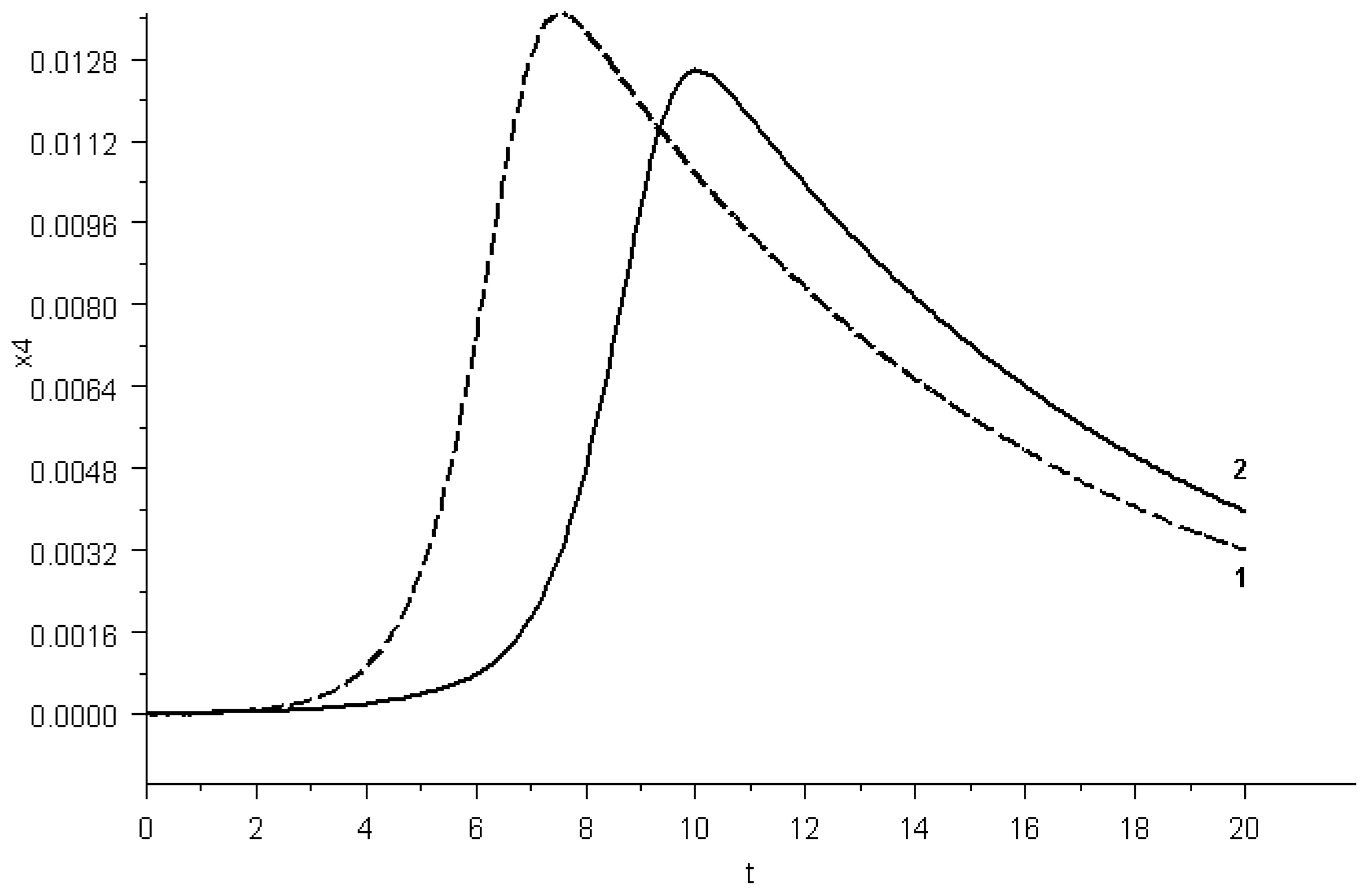
Example 1.

The comparative efficiency of the proposed fixed-point method is illustrated in a model example of the problem of optimal control of the immune process without delay. In accordance with works [7,9], the model of a controlled system in a dimensionless form can be represented as:

$$\begin{array}{c}{\dot{x}}_1=h_1{x}_1-h_2{x}_1{x}_2-u{x}_1,u\left(t\right)\in [0,u_{max}],t\in T=[0,t_1],\\ {\dot{x}}_2=h_4(x_3-x_2)-h_8{x}_1{x}_2,\\ {\dot{x}}_3=h_3{x}_1{x}_2-h_5(x_3-1),\\ {\dot{x}}_4=h_6{x}_1-h_7{x}_4,\\ x_1\left(0\right)=x_1^0>0,x_2\left(0\right)=1,x_3\left(0\right)=1,x_4\left(0\right)=0.\end{array}$$

(13)

The variable $x_1=x_1\left(t\right)$ characterizes the infectious pathogen (virus), and the variables $x_2=x_2\left(t\right)$, $x_3=x_3\left(t\right)$ characterize the organism’s defenses (antibodies and plasma cells, respectively). The variable $x_4=x_4\left(t\right)$ characterizes the degree of damage to the organism, $h_i>0$, $i=\overline{1,8}$ are given constant coefficients. The initial conditions simulate the situation of infection of the organism with a small initial dose of the virus $x_1^0$ at the initial moment $t=0$. The control $u\left(t\right),t\in T$ characterizes the intensity of the introduction of immunoglobulins that neutralize the virus.

The control $u\left(t\right)\equiv 0,t\in T$ corresponds to the case of no treatment using the introduction of immunoglobulins. This model situation corresponds to an acute illness with recovery at the following values of the coefficients [7]:

$$h_1=2,h_2=0.8,h_3={10}^4,h_4=0.17,h_5=0.5,$$

$$h_6=10,h_7=0.12,h_8=8,x_1^0={10}^{-6}.$$

The unit of time corresponds to one day.

The purpose of the control is to minimize the value of the virus by the end of treatment with the introduction of immunoglobulins with the condition of limiting the indicator of damage to the organism at a given time interval:

$${\Phi }_0\left(u\right)=x_1\left(t_1\right)\to inf,$$

$${\int }_T{x}_4\left(t\right)dt\le m,m>0.$$

(14)

The considered limitation (14) is important in modeling the acute form of a viral disease when the consequences of damage to the organism cannot be neglected.

The value of the maximum intensity of the control action was set equal to $u_{max}=0.5$. The time interval T was set to be equal to 20 days: $t_1=20$. The value of the maximum damage to the organism was chosen to be equal to $m=0.1$.

We introduce an additional variable according to the rule:

$${\dot{x}}_5=x_4,x_5\left(0\right)=0.$$

(15)

Then the integral constraint (14) reduces to the terminal constraint:

$$x_5\left(t_1\right)\le m,m>0.$$

In numerical calculations of the problem with constraint (14), the validity of the activity property of inequality (14) was established. As a result, the problem of the considered class was studied:

$$\begin{array}{c}{\Phi }_0\left(u\right)=x_1\left(t_1\right)\to inf,\end{array}$$

(16)

$$\begin{array}{c}{\Phi }_1\left(u\right)=x_5\left(t_1\right)-m=0,m>0.\end{array}$$

(17)

The Pontryagin function in problem (13), (15)–(17) is represented as:

$$H(p,x,u,t)=H_0(p,x,t)+H_1(p,x,t)u,$$

$$\begin{array}{c}{H}_0(p,x,t)=p_1(h_1{x}_1-h_2{x}_1{x}_2)+p_2(h_4(x_3-x_2)-h_8{x}_1{x}_2)+\\ +p_3(h_3{x}_1{x}_2-h_5(x_3-1))+p_4(h_6{x}_1-h_7{x}_{4}2)+p_5{x}_4,\end{array}$$

$$H_1(p,x,t)=-p_1{x}_1.$$

To solve problem (13), (15)–(17), we used the proposed method of fixed points (M2) based on the iterative process (12) and the well-known method of penalty functionals (M1) with the objective functional of the following form:

$$\Phi \left(u\right)={\Phi }_0\left(u\right)+{\gamma }_s{\Phi }_1^2\left(u\right)\to inf,$$

(18)

where ${\gamma }_s>0$, $s\ge 0$ is a given penalty parameter.

Auxiliary penalty problems (13), (15) and (18) were calculated using the well-known conditional gradient method [28]. As a criterion for stopping the calculation of the penalty problem for a fixed value of the penalty, parameter ${\gamma }_s>0$ condition was chosen:

$$|\Phi \left(u^{k+1}\right)-\Phi \left(u^k\right)|<{\epsilon }_1|\Phi \left(u^k\right)|,$$

(19)

where $k>0$ is an iterative index of the conditional gradient method, ${\epsilon }_1={10}^{-5}$.

After reaching stopping criterion (19), the fulfillment of the terminal constraint was checked:

$$|x_5(t_1,u^{k+1})-m|<{\epsilon }_2,$$

(20)

where ${\epsilon }_2={10}^{-4}$ is the specified accuracy.

If condition (20) was not satisfied, then a new penalty problem was calculated with the penalty parameter:

$${\gamma }_{s+1}=\beta {\gamma }_s,\beta =10.$$

The initial value of the penalty parameter ${\gamma }_0$ was set equal to ${10}^{-10}$.

When calculating a new penalty problem using the conditional gradient method, the resulting computational control in the previous penalty problem was chosen as the initial approximation. The calculation using the M1 method ended with the simultaneous fulfillment of conditions (19) and (20).

To implement the proposed method M2, we consider the auxiliary regular Lagrange functional with a multiplier $\lambda \in R$:

$$L(u,\lambda )=x_1\left(t_1\right)+\lambda (x_5\left(t_1\right)-m).$$

The modified conjugate system (6) takes the form:

$$\begin{array}{c}{\dot{p}}_1=-h_1{p}_1+h_2{x}_2{p}_1+p_{1}u+h_8{x}_2{p}_2-h_3{x}_2{p}_3-h_6{p}_4+\frac{1}{2}(h_2{p}_1+h_8{p}_2-h_3{p}_3)z_2,\\ {\dot{p}}_2=h_2{x}_1{p}_1+h_4{p}_2+h_8{x}_1{p}_2-h_3{x}_1{p}_3+\frac{1}{2}(h_2{p}_1+h_8{p}_2-h_3{p}_3)z_1,\\ {\dot{p}}_3=-h_4{p}_2+h_5{p}_3,\\ {\dot{p}}_4=h_7{p}_4-p_5,\\ {\dot{p}}_5=0,\\ p_1\left(t_1\right)=-1,p_2\left(t_1\right)=p_3\left(t_1\right)=p_4\left(t_1\right)=0,p_5\left(t_1\right)=-\lambda .\end{array}$$

For available controls $u^0,v$, the function $p(t,u^0,v,\lambda )$, $t\in T$ is the solution of the modified conjugate system for $u=u^0\left(t\right)$, $x_i=x_i(t,u^0)$, $z_i=x_i(t,v)-x_i(t,u^0)$, $i=1,2$.

Auxiliary vector function $u^{\alpha }(p,x,t)$ based on the projecting operation is determined with the formula:

$$u^{\alpha }(p,x,t)=\left\{\begin{array}{c}{u}_{max},u^0\left(t\right)-\alpha p_1{x}_1>u_{max},\\ u^0\left(t\right)-\alpha p_1{x}_1,0\le u^0\left(t\right)-\alpha p_1{x}_1\le u_{max},\\ 0,u^0\left(t\right)-\alpha p_1{x}_1<0.\end{array}\right.$$

The fixed-point problem (9) to improve the available control $u^0$ takes the form:

$$\begin{array}{c}v\left(t\right)=u^{\alpha }(p(t,u^0,v,\lambda ),x(t,v),t),t\in T,\lambda \in R,\\ {\Phi }_1\left(v\right)=x_5(t_1,v)-m=0.\end{array}$$

(21)

For a given $\alpha >0$ iterative process (12) for $k\ge 0$ with an initial available control $v^0$ for $k=0$ has the form:

$$\begin{array}{c}{v}^{k+1}\left(t\right)=u^{\alpha }(p(t,u^0,v^k,\lambda ),x(t,v^{k+1}),t),t\in T,\lambda \in R,\\ {\Phi }_1\left(v^{k+1}\right)=x_5(t_1,v^{k+1})-m=0.\end{array}$$

(22)

At each iteration of process (22), a special Cauchy problem is solved:

$$\begin{array}{c}{\dot{x}}_1\left(t\right)=h_1{x}_1\left(t\right)-h_2{x}_1\left(t\right)x_2\left(t\right)-u^{\alpha }(p(t,u^0,v^k,\lambda ),x\left(t\right),t)x_1\left(t\right),\\ {\dot{x}}_2\left(t\right)=h_4(x_3\left(t\right)-x_2\left(t\right))-h_8{x}_1\left(t\right)x_2\left(t\right),\\ {\dot{x}}_3\left(t\right)=h_3{x}_1\left(t\right)x_2\left(t\right)-h_5(x_3\left(t\right)-1),\\ {\dot{x}}_4\left(t\right)=h_6{x}_1\left(t\right)-h_7{x}_4\left(t\right),\\ {\dot{x}}_5\left(t\right)=x_4\left(t\right),\\ x_1\left(0\right)=x_1^0>0,x_2\left(0\right)=1,x_3\left(0\right)=1,x_4\left(0\right)=0,x_5\left(0\right)=0,\end{array}$$

with the simultaneous calculation of the auxiliary control:

$$v^{k+1}\left(t\right)=u^{\alpha }(p(t,u^0,v^k,\lambda ),x\left(t\right),t),t\in T,\lambda \in R.$$

The resulting control, which depends on the Lagrange multiplier, satisfies the first equation of system (22).

To solve the corresponding algebraic equation of system (22) with respect to the Lagrange multiplier, the dumpol procedure from the Fortran software package [29] was used, which implemented the deformable polyhedron method. The accuracy of solving the equation was chosen to be equal to ${10}^{-4}$, which corresponded to the accuracy of criterion (20).

For a given $\alpha >0$ iterative process (22) was carried out until the first fulfillment of the condition:

$${\Phi }_0\left(u^{k+1}\right)<{\Phi }_0\left(u^k\right).$$

In this case, to improve the resulting control, a new problem (21) and algorithm (22) were constructed. In this case, as an initial approximation of the control at $k=0$ for iterative process (22), the resulting computational control was chosen.

Thus, starting from the second computational improvement problem (21), the sequence of computational controls forms a relaxation sequence of controls that satisfy constraint (17) with a given accuracy.

If a strict improvement of the control in the process of iterations (22) was not achieved, then the numerical calculation of fixed-point problem (21) was carried out until the condition:

$$|{\Phi }_0\left(u^{k+1}\right)-{\Phi }_0\left(u^k\right)|<{\epsilon }_3\left|{\Phi }_0\left(u^k\right)\right|,$$

where ${\epsilon }_3={10}^{-5}$. This was the end of the construction and calculation of sequential fixed-point problems for improving control.

As a starting initial approximation in both methods M1 and M2, the control $u\left(t\right)\equiv 0,t\in T$ was chosen.

The comparative results of calculations using the considered methods are shown in

Table 1. Quantitative indicators of calculations for methods M1 and M2.

Method	${\mathbf{\Phi }}_{\mathbf{0}}$	$|{\mathbf{\Phi }}_{\mathbf{1}}|$	N	Note
M1	2.686698 × 10−19	1.854861 × 10−5	464	10−6
M2	1.172261 × 10−20	1.534792 × 10−5	88	103

in which ${\Phi }_0$ is the calculated value of the objective functional of the problem, $|{\Phi }_1|$ is the modulus of the calculated value of the functional corresponding to constraint (17), and N is the total number of solved Cauchy problems. The note for the M1 method gives the value of the penalty parameter, which provided the specified accuracy of the terminal constraint (20). For proposed method M2, the note indicates the specified value of projection parameter $\alpha >0$, which ensures the convergence of the iterative process (22).

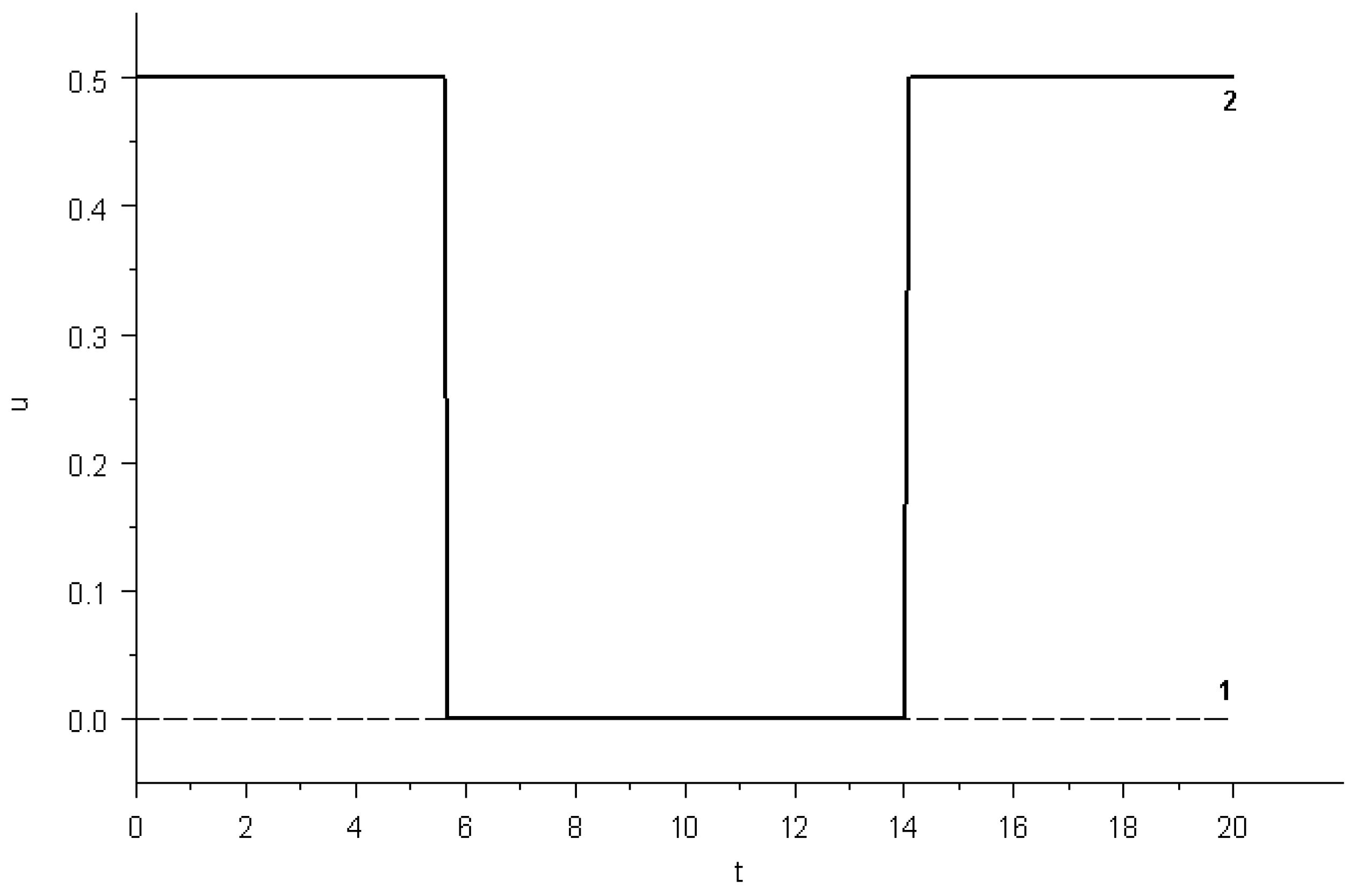
The computational control in methods M1 and M2 is a piecewise-constant function with an accuracy of up to a day with a switching point at the moment $t=5$ from the maximum value $u_{max}=0.5$ to the minimum value equal to zero with reverse switching at moment $t=14$.

Figure 1, Figure 2, Figure 3, Figure 4, Figure 5 and Figure 6 show approximate graphs of the computational control and the corresponding phase variables with a time discretization step equal to $0.1$.

According to the optimal strategy for the treatment of an acute disease, taking into account the limitation of the severity of the disease, it is necessary to administer immunoglobulins with maximum intensity at the initial stage of the disease in order to reduce the severity of the disease when the organism’s immune response is still weak. Then, as the organism’s defenses are formed, it is necessary to stop the administration of the drug so that the immune response is formed in full force by the type of feedback on the pathogen. At the last stage, corresponding to the recovery of the organism, immunoglobulins must be administered again with maximum intensity in order to achieve a minimization of the virus value by the end of the specified treatment interval. Previously, a similar strategy for treating the disease using the exacerbation method was proposed and tested in the course of the computational model experiments in [7]. The formulation of tasks for the optimal management of the treatment of a disease makes it possible to substantiate and effectively regulate the process of treatment using the exacerbation method.

Within the framework of a model example, the proposed method of fixed points provides a significant reduction in computational complexity compared to the standard method of penalty functionals, which is estimated using the total number of Cauchy computational problems.

Example 2.

The comparative efficiency of the proposed fixed-point method is illustrated with the example of the well-known model problem of satellite rotation stabilization [30,31], which is considered in the following formulation:

$$\begin{array}{c}\begin{array}{c}{\dot{x}}_1=\frac{1}{3}{x}_2{x}_3+100u_1,t\in T=[0,t_1],t_1=0.1,\\ {\dot{x}}_2=-x_1{x}_3+25u_2,\\ {\dot{x}}_3=-x_1{x}_2+100u_3,\\ x_1\left(0\right)=200,x_2\left(0\right)=30,x_3\left(0\right)=40,\\ |u_1\left(t\right)|\le 40,|u_2\left(t\right)|\le 20,|u_3\left(t\right)|\le 40,t\in T,\end{array}\end{array}$$

(23)

$$\begin{array}{c}{\Phi }_0\left(u\right)=\frac{1}{2}(x_2^2\left(t_1\right)+x_3^2\left(t_1\right))\to inf,\end{array}$$

(24)

$$\begin{array}{c}{\Phi }_1\left(u\right)=x_1\left(t_1\right)=0.\end{array}$$

(25)

The equations of the system describe the dynamics of the rotation of a satellite equipped with three jet engines. The controls characterize fuel consumption. The minimized functional from the control reflects the goal of achieving a state characterized by the absence of satellite rotation (stabilization).

The Pontryagin function in problem (23)–(25) is represented as:

$$H(p,x,u,t)=H_0(p,x,t)+H_{11}(p,x,t)u_1+H_{12}(p,x,t)u_2+H_{13}(p,x,t)u_3,$$

$$H_0(p,x,t)=\frac{1}{3}{p}_1{x}_2{x}_3-p_2{x}_1{x}_3-p_3{x}_1{x}_2,$$

$$H_{11}(p,x,t)=100p_1,H_{12}(p,x,t)=25p_2,H_{13}(p,x,t)=100p_3.$$

To solve problem (23)–(25), we used the proposed method of fixed points (M3) based on the iterative process (12) and the known method of penalty functionals with the objective functional in the following form:

$$\Phi \left(u\right)={\Phi }_0\left(u\right)+{\gamma }_s{\Phi }_1^2\left(u\right)\to inf,$$

(26)

where ${\gamma }_s>0$, $s\ge 0$ is a given penalty parameter.

Auxiliary penalty problems (23) and (26) were calculated using the well-known conditional gradient method (M1) and gradient projection method (M2) [28]. As a criterion for stopping the calculation of the penalty problem for a fixed value of the penalty parameter, the following condition was chosen:

$$|\Phi \left(u^{k+1}\right)-\Phi \left(u^k\right)|<{\epsilon }_1|\Phi \left(u^k\right)|,$$

(27)

where $k>0$ is an iterative index of conditional gradient and gradient projection methods, ${\epsilon }_1={10}^{-5}$.

After reaching the stopping criterion (27), the fulfillment of the terminal constraint was checked:

$$|x_1(t_1,u^{k+1})|<{\epsilon }_2,$$

(28)

where ${\epsilon }_2={10}^{-6}$ is the specified accuracy.

If condition (28) was not satisfied, then a new penalty problem was calculated with the penalty parameter:

$${\gamma }_{s+1}=\beta {\gamma }_s,\beta =10.$$

The initial value of the penalty parameter ${\gamma }_0$ was set equal to $0.5$.

When calculating a new penalty problem using the M1 and M2 methods, the resulting computational control in the previous penalty problem was chosen as the initial approximation. The calculation using methods M1 and M2 ended when conditions (27) and (28) were simultaneously satisfied.

To implement the proposed M3 method, an auxiliary regular Lagrange functional with the multiplier $\lambda \in R$ was considered:

$$L(u,\lambda )=\frac{1}{2}(x_2^2\left(t_1\right)+x_3^2\left(t_1\right))+\lambda x_1\left(t_1\right).$$

First, problems (23)–(25) were reduced to forms (1)–(3) by introducing an auxiliary variable $x_4\left(t\right)=\frac{1}{2}(x_2^2\left(t\right)+x_3^2\left(t\right))$. After compiling the modified conjugate system and excluding the corresponding conjugate variable $p_4\left(t\right)$ from it, the modified conjugate system takes the form:

$$\begin{array}{c}{\dot{p}}_1=p_2{x}_3+p_3{x}_2+\frac{1}{2}(p_3{z}_2+p_2{z}_3),\\ {\dot{p}}_2=-\frac{1}{3}{p}_1{x}_3+p_3{x}_1+\frac{1}{2}(p_3{z}_1-\frac{1}{3}{p}_1{z}_3),\\ {\dot{p}}_3=-\frac{1}{3}{p}_1{x}_2+p_2{x}_1+\frac{1}{2}(p_2{z}_1-\frac{1}{3}{p}_1{z}_2),\\ p_1\left(t_1\right)=-\lambda ,p_2\left(t_1\right)=-x_2\left(t_1\right)-\frac{1}{2}{z}_2\left(t_1\right),p_3\left(t_1\right)=-x_3\left(t_1\right)-\frac{1}{2}{z}_3\left(t_1\right).\end{array}$$

For available controls $u^0,v$, the function $p(t,u^0,v,\lambda )$, $t\in T$ is the solution of the modified conjugate system for $x_i=x_i(t,u^0)$, $z_i=x_i(t,v)-x_i(t,u^0)$, $i=1,2,3$.

Auxiliary vector function $u^{\alpha }(p,x,t)$ based on the projecting operation is determined with the formula:

$$u^{\alpha }(p,x,t)=\left(\begin{array}{c}{u}_1^{\alpha }(p,x,t)\\ u_2^{\alpha }(p,x,t)\\ u_3^{\alpha }(p,x,t)\end{array}\right),$$

where

$$u_1^{\alpha }(p,x,t)=\left\{\begin{array}{c}40,u^0\left(t\right)+100\alpha p_1>40,\\ u^0\left(t\right)+100\alpha p_1,-40\le u^0\left(t\right)+100\alpha p_1\le 40,\\ -40,u^0\left(t\right)+100\alpha p_1<-40,\end{array}\right.$$

$$u_2^{\alpha }(p,x,t)=\left\{\begin{array}{c}20,u^0\left(t\right)+25\alpha p_2>20,\\ u^0\left(t\right)+25\alpha p_2,-20\le u^0\left(t\right)+25\alpha p_2\le 20,\\ -20,u^0\left(t\right)+25\alpha p_2<-20,\end{array}\right.$$

$$u_3^{\alpha }(p,x,t)=\left\{\begin{array}{c}40,u^0\left(t\right)+100\alpha p_3>40,\\ u^0\left(t\right)+100\alpha p_3,-40\le u^0\left(t\right)+100\alpha p_3\le 40,\\ -40,u^0\left(t\right)+100\alpha p_3<-40.\end{array}\right.$$

Fixed-point problem (9) to improve the available control $u^0$ takes the form:

$$\begin{array}{c}v\left(t\right)=u^{\alpha }(p(t,u^0,v,\lambda ),x(t,v),t),t\in T,\lambda \in R,\\ {\Phi }_1\left(v\right)=x_1(t_1,v)=0.\end{array}$$

(29)

For a given $\alpha >0$ iterative process (12) for $k\ge 0$ with an initial available control $v^0$ for $k=0$ has the form:

$$\begin{array}{c}{v}^{k+1}\left(t\right)=u^{\alpha }(p(t,u^0,v^k,\lambda ),x(t,v^{k+1}),t),t\in T,\lambda \in R,\\ {\Phi }_1\left(v^{k+1}\right)=x_1(t_1,v^{k+1})=0.\end{array}$$

(30)

At each iteration of process (30), a special Cauchy problem is solved:

$$\begin{array}{c}{\dot{x}}_1=\frac{1}{3}{x}_2{x}_3+100u_1^{\alpha }(p(t,u^0,v^k,\lambda ),x,t),t\in T=[0,t_1],\\ {\dot{x}}_2=-x_1{x}_3+25u_2^{\alpha }(p(t,u^0,v^k,\lambda ),x,t),\\ {\dot{x}}_3=-x_1{x}_2+100u_3^{\alpha }(p(t,u^0,v^k,\lambda ),x,t),\\ x_1\left(0\right)=200,x_2\left(0\right)=30,x_3\left(0\right)=40\end{array}$$

with the simultaneous calculation of the auxiliary control:

$$v^{k+1}\left(t\right)=u^{\alpha }(p(t,u^0,v^k,\lambda ),x\left(t\right),t),t\in T,\lambda \in R.$$

The received control, which depends on the Lagrange multiplier, satisfies the first equation of system (30).

To solve the corresponding algebraic equation of system (30) with respect to the Lagrange multiplier, the dumpol procedure from the Fortran software package [29] was used, which implements the deformable polyhedron method. The accuracy of solving the equation was chosen equal to ${10}^{-6}$, which corresponds to the accuracy of criterion (28).

For a given $\alpha >0$, iterative process (30) was carried out until the first fulfillment of the condition:

$${\Phi }_0\left(u^{k+1}\right)<{\Phi }_0\left(u^k\right).$$

In this case, to improve the resulting control, a new problem (29) and algorithm (30) were constructed. In this case, as an initial approximation of the control at $k=0$ for the iterative process (30), the resulting computational control was chosen.

Thus, starting from the second computational improvement problem (29), the sequence of computational controls forms a relaxation sequence of controls that satisfy constraint (25) with a given accuracy.

If a strict improvement of the control in the process of iterations (30) was not achieved, then the numerical calculation of the fixed-point problem (29) was carried out until the condition:

$$|{\Phi }_0\left(u^{k+1}\right)-{\Phi }_0\left(u^k\right)|<{\epsilon }_3\left|{\Phi }_0\left(u^k\right)\right|,$$

where ${\epsilon }_3={10}^{-5}$. This was the end of the construction and calculation of sequential fixed-point problems for improving control.

As a starting initial approximation in all methods, we chose the control $u\left(t\right)\equiv 0,t\in T$.

Comparative results of calculations using the considered methods are shown in

Table 2. Quantitative indicators of calculations for methods M1, M2 and M3.

Method	${\mathbf{\Phi }}_{\mathbf{0}}$	$|{\mathbf{\Phi }}_{\mathbf{1}}|$	N	Note
M1	3.16428 × 10−13	2.45074 × 10−7	8512	0.5
M2	1.48471 × 10−13	3.13041 × 10−7	2642	0.5
M3	3.63122 × 10−13	5.22914 × 10−8	1458	10−5

in which ${\Phi }_0$ is the calculated value of the objective functional of the problem, $|{\Phi }_1|$ is the modulus of the calculated value of the functional corresponding to constraint (25), N is the total number of solved Cauchy problems. The note for the M1 and M2 methods gives the value of the penalty parameter, which provided the specified accuracy of the terminal constraint (25). For proposed method M3, the note indicates the specified value of the projection parameter $\alpha >0$, which ensures the convergence of the iterative process (30).

In the framework of Example 2 with multidimensional control, the proposed method of fixed points provides a significant reduction in the computational complexity, which is estimated by the total number of Cauchy computational problems compared to the known gradient methods based on penalty functionals.

Example 3.

The considered example illustrates the possibility of the rigorous improvement of a non-optimal control that satisfies the maximum principle using the proposed fixed-point method. Gradient methods do not have this capability.

$$\begin{array}{c}\dot{x}\left(t\right)=u\left(t\right),x\left(0\right)=0,\left|u\left(t\right)\right|\le 20,t\in T=[0,\pi ],\\ {\Phi }_0\left(u\right)=-\underset{0}{\overset{\pi }{\int }}{x}^{2}dt\to inf,\\ {\Phi }_1\left(u\right)=x\left(\pi \right)=0.\end{array}$$

The Pontryagin function has the form:

$$H=pu+x^2,H_0=x^2,H_1=p.$$

For a control $u^0\in V$ and a given parameter $\alpha >0$, an auxiliary vector function $u^{\alpha }(p,x,t)$ based on the projecting operation takes the form:

$$u^{\alpha }(p,x,t)=\left\{\begin{array}{c}20,u^0\left(t\right)+\alpha p>20,\\ u^0\left(t\right)+\alpha p,-20\le u^0\left(t\right)+\alpha p\le 20,\\ -20,u^0\left(t\right)+\alpha p<-20.\end{array}\right.$$

A simple analysis of the problem, taking into account its reduction to the form (1)–(3) shows that the problem under consideration is non-degenerate and the maximum principle condition for control $u\in W$ for some $\lambda \in R$ can be represented in the following projection form:

$$u\left(t\right)=u^{\alpha }(\psi (t,u,\lambda ),x(t,u),t),$$

where the function $\psi (t,u,\lambda )$, $t\in T$ is the solution of the standard conjugate system:

$$\dot{\psi }\left(t\right)=-2x\left(t\right),\psi \left(\pi \right)=-\lambda$$

for $x\left(t\right)=x(t,u)$, $t\in T$. The control $u^0\left(t\right)=0$, $t\in T$, is a non-optimal extremal control. Wherein $x(t,u^0)\equiv 0$, $t\in T$, ${\Phi }_0\left(u^0\right)=0$.

The improvement problem for control $u^0\in V$ based on the regular Lagrange functional $L(u,\lambda )={\Phi }_0\left(u\right)+\lambda {\Phi }_1\left(u\right)$ has the following form:

$$\begin{array}{c}v\left(t\right)=u^{\alpha }(p(t,u^0,v,\lambda ),x(t,v),t),t\in T,\lambda \in R,\\ {\Phi }_1\left(v\right)=x(\pi ,v)=0,\end{array}$$

(31)

where the function $p(t,u^0,v,\lambda )$, $t\in T$ is the solution of the modified conjugate system:

$$\dot{p}\left(t\right)=-2x\left(t\right)-z\left(t\right),p\left(\pi \right)=-\lambda$$

for $x\left(t\right)=x(t,u^0)$, $z\left(t\right)=x(t,v)-x(t,u^0)$, $t\in T$. From this we obtain that for the extremal control $u^0\left(t\right)=0$, $t\in T$ the function $p(t,u^0,v,\lambda )$, $t\in T$ is the solution of the modified conjugate system:

$$\dot{p}\left(t\right)=-z\left(t\right),p\left(\pi \right)=-\lambda$$

for $z\left(t\right)=x(t,v)$, $t\in T$.

System (31) for improving the extremal control $u^0\left(t\right)=0$, $t\in T$ is an equivalent boundary value problem:

$$\begin{array}{c}\dot{x}\left(t\right)=u^{\alpha }(p,x,t),x\left(0\right)=x\left(\pi \right)=0,\\ \dot{p}\left(t\right)=-x\left(t\right),p\left(\pi \right)=-\lambda .\end{array}$$

In accordance with Theorem 3, the pair of functions $\psi (t,u^0,\lambda )=0$, $x\left(t\right)=x(t,u^0)=0$, $t\in T$ with $\lambda =0$ is an obvious solution to this boundary value problem.

A simple analysis shows that this boundary value problem for $\alpha =1$ has solutions of the following form with $\lambda =C$:

$$p\left(t\right)=Ccost,x\left(t\right)=Csint,\left|C\right|\le 20,t\in T.$$

These solutions of the boundary value problem correspond to the solutions of system (31):

$$v\left(t\right)=Ccost,t\in T$$

with the corresponding values of the objective functional ${\Phi }_0\left(v\right)=-\frac{\pi }{2}{C}^2$.

Thus, system (31) at $\alpha =1$ for extremal control $u^0=0$ has a non-unique solution, and extremal control $u^0=0$ is strictly improved on other solutions of system (31) at $0<\left|C\right|\le 20$.

Let us show the possibility of a rigorous improvement of the extremal control $u^0=0$ using the proposed fixed-point method with the parameter $\alpha =1$.

The iterative process for solving system (31) takes the form

$$\begin{array}{c}{v}^{k+1}\left(t\right)=u^{\alpha }(p(t,u^0,v^k,\lambda ),x(t,v^{k+1}),t),t\in T,\lambda \in R,\\ {\Phi }_1\left(v^{k+1}\right)=x(\pi ,v^{k+1})=0.\end{array}$$

(32)

As an initial approximation of the iterative process (32), we consider the available control $v^0\left(t\right)\equiv -6$, $t\in T$, which corresponds to the phase trajectory $x(t,v^0)=-6t$, $t\in T$. In that case, the function $p(t,u^0,v^0,t)$, $t\in T$ is the solution of the modified conjugate equation:

$$\dot{p}\left(t\right)=6t,p\left(\pi \right)=-\lambda .$$

The solution to this equation is the function:

$$p(t,u^0,v^0,t)=3t^2-\lambda -3{\pi }^2,t\in T.$$

Let us assume that $\left|p\right(t,u^0,v^0,\lambda \left)\right|\le 20$, $t\in T$. Then the corresponding Cauchy problem for the phase system takes the form:

$$\dot{x}=3t^2-\lambda -3{\pi }^2,x\left(0\right)=0.$$

The solution to this equation is the function:

$$x\left(t\right)=t^3-(\lambda +3{\pi }^2)t,t\in T.$$

The condition $x(\pi ,v^1)=0$ determines the value of the Lagrange multiplier $\overline{\lambda }=-2{\pi }^2$. This gives us a function:

$$p(t,u^0,v^0,t)=3t^2-{\pi }^2,t\in T,$$

which satisfies the condition $\left|p\right(t,u^0,v^0,\overline{\lambda }\left)\right|\le 20$, $t\in T$.

From here, we get the control:

$$v^1\left(t\right)=3t^2-{\pi }^2,t\in T.$$

This control corresponds to the phase trajectory $x(t,v^1)=t^3-{\pi }^{2}t$, $t\in T$ and the value of the objective functional:

$${\Phi }_0\left(v^1\right)=-\frac{8}{105}{\pi }^7\approx -230.118<{\Phi }_0\left(u^0\right)=0.$$

Thus, the fixed-point method already at the first iteration makes it possible to strictly improve the non-optimal extremal control $u^0=0$. The possibility of a rigorous improvement of the extremal control appears due to the available choice of the starting initial control $v^0\in V$, which differs from the extremal control. There is no such choice in gradient methods.

5. Conclusions

Let us single out the difference between the proposed fixed-point approach and the well-known Lagrange approach in problems with constraints. The Lagrange method is based on the necessary conditions for the optimality of control (Pontryagin’s maximum principle) in problems with constraints, represented by the generalized Lagrange functional. The proposed method of fixed points is based on the conditions for improving control, represented by the regular Lagrange functional in the form of a fixed-point problem in the control space. The developed conditions for improving control in the form of a fixed-point problem make it possible to apply and modify the known theory and methods of fixed points to find a solution to the considered polynomial optimal control problems with constraints.

The proposed method of fixed points is characterized by the property of non-local improvement of control; the possibility of rigorous improvement of non-optimal controls that satisfy the maximum principle; the absence of a control variation procedure, which is typical for gradient methods; precise fulfillment of constraints at each iteration of the method; the presence of one main tuning projection parameter $\alpha >0$, which regulates the speed, quality, and area of convergence of the iterative process. These properties are important for improving the efficiency of solving polynomial optimal control problems with constraints compared to known methods.

One of the main limitations of the application of the proposed method is the assumption that at each iteration of the method, the corresponding algebraic equation is solvable with respect to the Lagrange multiplier. In cases where, at some iterations of the proposed method, the indicated algebraic equation is unsolvable, a generalized modification of the method can be used, which consists in finding the Lagrange multiplier that minimizes the modulus of the restriction functional.

The proposed optimization approach based on constructing control improvement conditions in the form of fixed-point problems can be extended to other polynomial optimal control problems, including those with delays, mixed control functions and parameters, piecewise constant controls, and other features. In particular, it is planned to develop a modification of the proposed fixed-point method for polynomial optimal control problems with constant delays, which are typical for models of the immune process in diseases.

References

1. Modeling the Socio-Ecological-Economic System of a Region; Gurman, V.; Ryumina, E. (Eds.) Nauka: Moscow, Russia, 2001; pp. 1–175. [Google Scholar]
2. Modeling and Control of Regional Development Processes; Vasiliev, S. (Ed.) Fizmatlit: Moscow, Russia, 2001; pp. 1–432. [Google Scholar]
3. Proops, J.; Safonov, P. Modeling in Ecological Economics; Edward Elgar: Cheltenham, UK, 2004; pp. 1–203. [Google Scholar]
4. Marry, J. Nonlinear Differential Equations in Biology. Lectures on Models; Mir: Moscow, Russia, 1983; pp. 1–397. [Google Scholar]
5. Riznichenko, G. Lectures on Mathematical Models in Biology; Regulyarnaya i Khaoticheskaya Dinamika: Izhevsk, Russia, 2002; pp. 1–232. [Google Scholar]
6. Bratus, A.; Novozhilov, A.; Platonov, A. Dynamic Systems and Models in Biology; Fizmatlit: Moscow, Russia, 2010; pp. 1–400. [Google Scholar]
7. Marchuk, G. Mathematical Models of Immune Response in Infections Diseases; Kluwer Press: Dordrecht, The Netherlands, 1997; pp. 1–360. [Google Scholar]
8. Shestakov, A.; Sviridyuk, G.; Keller, A.; Zamyshlyaeva, A.; Khudyakov, Y. Numerical investigation of optimal dynamic measurements. Acta IMEKO 2018, 7, 65–72. [Google Scholar] [CrossRef]
9. Kabanikhin, S.; Krivorot’ko, O. Optimization methods for solving inverse immunology and epidemiology problems. Comput. Math. Math. Phys. 2020, 60, 580–589. [Google Scholar] [CrossRef]
10. Nduka, M.; Oruh, B. A Fermat polynomial method for solving optimal control problems. IJMAM Int. J. Math. Anal. Model. 2022, 5, 56–68. [Google Scholar]
11. Gerbet, D.; Röbenack, K. A high-gain observer for embedded polynomial dynamical systems. Mathematics 2023, 11, 190. [Google Scholar] [CrossRef]
12. Guo, M.; De Persis, C.; Tesi, P. Data-driven stabilization of nonlinear polynomial systems with noisy data. IEEE Trans. Autom. Control 2022, 67, 4210–4217. [Google Scholar] [CrossRef]
13. Shumafov, M. Stabilization of linear control systems and pole assignment problem: A survey. Vestnik St. Petersburg Univ. Math. 2019, 6, 564–591. [Google Scholar]
14. Warrad, B.I.; Bouafoura, M.K.; Braiek, N.B. Tracking control design for nonlinear polynomial systems via augmented error system approach and block pulse functions technique. Kybernetika 2019, 55, 831–851. [Google Scholar]
15. Baillieul, J. Controllability and observability of polynomial dynamical systems. Nonlinear Anal. Theory Meth. Appl. 1981, 5, 543–552. [Google Scholar] [CrossRef]
16. Chen, C. Explicit solutions and stability properties of homogeneous polynomial dynamical systems. IEEE Trans. Autom. Control 2022, 1–8. [Google Scholar] [CrossRef]
17. Ahmadi, A.A.; El Khadir, B. On algebraic proofs of stability for homogeneous vector fields. IEEE Trans. Autom. Control 2020, 65, 325–332. [Google Scholar] [CrossRef] [Green Version]
18. Chukanov, S.; Chukanov, I. The investigation of nonlinear polynomial control systems. MAIS 2021, 28, 238–249. [Google Scholar] [CrossRef]
19. Xiao, B.; Lam, H.-K.; Zhong, Z. Iterative stability analysis for general polynomial control systems. Nonlinear Dyn. 2021, 105, 3139–3148. [Google Scholar] [CrossRef]
20. Roitenberg, V. On generic polinomial differential equations of second order on the circle. Sib. Elektron. Mat. Izv. 2020, 17, 2122–2130. [Google Scholar] [CrossRef]
21. Zaytsev, M.; Akkerman, V. Explicit transformation of the Riccati equation and other polynomial ODEs to systems of linear ODEs. Tomsk State Univ. J. Math. Mech. 2021, 72, 5–14. [Google Scholar] [CrossRef]
22. Yousif, A.; Qasim, A. A novel iterative method based on Bernstein-Adomian polynomials to solve non-linear differential equations. Open Access Libr. J. 2020, 7, e6267. [Google Scholar] [CrossRef]
23. Changhuang, W.; Ran, D.; Ping, L. Alternating minimization algorithm for polynomial optimal control problems. J. Guid. Control Dyn. 2019, 42, 723–736. [Google Scholar]
24. Arguchintsev, A.; Srochko, V. Procedure for Regularization of Bilinear Optimal Control Problems Based on a Finite-Dimensional Model; St Petersburg State University: St Petersburg, Russia, 2022; Volume 18, pp. 179–187. [Google Scholar]
25. Srochko, V. Iterative Methods for Solving Optimal Control Problems; Fizmatlit: Moscow, Russia, 2000; pp. 1–160. [Google Scholar]
26. Buldaev, A. Perturbation Methods in Problem of the Improvement and Optimization of the Controlled Systems; Buryat State University: Ulan-Ude, Russia, 2008; pp. 1–260. [Google Scholar]
27. Buldaev, A. A boundary improvement problem for linearly controlled processes. Autom. Remote Control 2011, 72, 1221–1228. [Google Scholar] [CrossRef]
28. Vasiliev, O. Optimization Methods; World Federation Publishers Company INC.: Atlanta, GA, USA, 1996; pp. 1–276. [Google Scholar]
29. Bartenev, O. Fortran for Professionals. IMSL Mathematical Library. Part 2; Dialog-MIFI: Moscow, Russia, 2001; pp. 1–320. [Google Scholar]
30. Tyatushkin, A. Numerical Methods and Software Tools for Optimization of Controlled Systems; Nauka: Novosibirsk, Russia, 1992; pp. 1–192. [Google Scholar]
31. Fedorenko, R. Approximate Solution of Optimal Control Problems; Nauka: Moscow, Russia, 1978; pp. 1–488. [Google Scholar]
Figure 1. 1—control u = 0 ; 2—computational control u.
Mathematics 11 01695 g001
Figure 2. 1—trajectory lg x 1 for u = 0 ; 2—computational trajectory lg x 1 .
Mathematics 11 01695 g002
Figure 3. 1—trajectory x 2 for u = 0 ; 2—computational trajectory x 2 .
Mathematics 11 01695 g003
Figure 4. 1—trajectory x 3 for u = 0 ; 2—computational trajectory x 3 .
Mathematics 11 01695 g004
Figure 5. 1—trajectory x 4 for u = 0 ; 2—computational trajectory x 4 .
Mathematics 11 01695 g005
Figure 6. 1—trajectory x 5 for u = 0 ; 2—computational trajectory x 5 .
Mathematics 11 01695 g006