Hybrid Impulsive Pinning Control for Mean Square Synchronization of Uncertain Multi-Link Complex Networks with Stochastic Characteristics and Hybrid Delays

Abstract

This study explores the synchronization issue for uncertain multi-link complex networks incorporating stochastic characteristics and hybrid delays. Unlike previous works, internal delays, coupling delays, and stochastic delays considered in our model change over time; meanwhile, the impulse strength and position change with time evolution. To actualize network synchronization, a strategy called hybrid impulsive pinning control is applied, which combines the virtue of impulsive control and pinning control as well as two categories of impulses (i.e., synchronization and desynchronization). By decomposing the complicated topological structures into diagonal items and off-diagonal items, multiple nonlinear coupling terms are linearly decomposed in the process of theoretical analysis. Combining inequality technology and matrix decomposition theory, several novel synchronization criteria have been gained to ensure synchronization for the concerning multi-link model. The criteria get in touch with the uncertain strengths, coupling strengths, hybrid impulse strengths, delay sizes, impulsive intervals, and network topologies.

1. Introduction

People generally live in various complex networks, such as transportation networks, information networks, power grids, and so on. Synchronization is a representative collective behavior of complex networks, which has a prominent theoretical meaning and extensive practical applications in non-fragile filtering, topology recognition, system stability, encryption, and decryption [1,2,3,4,5]. Recently, numerous synchronization modes have been discussed in depth, incorporating complete synchronization [6,7], cluster synchronization [8,9], quasi-synchronization [10,11], projective synchronization [12,13], exponential synchronization [14,15,16], etc. Regrettably, considering a complex network could have multi-links, many publications for synchronization analysis mainly concern complex networks including only a single link, making it difficult to portray the real network precisely. Multi-links mean that there may exist more than one path between each pair of nodes and that each pair has its special attributes. For instance, in the transportation networks, there are significant differences in carriage delays and connectivities among aviation networks, land networks, and waterway networks, which indicates single-link systems cannot characterize such types of multichannel transportation networks well (see Figure 1). For a human connection network, there are different communication tools, including e-mail, telephone, and Facebook. Obviously, this network represents a characteristic multi-link model that cannot be expressed by a single-link system. Hence, it is necessary to further study multi-links systems owing to their universality. Recently, some scholars have noticed various synchronization problems in such networks [17,18,19]. In [17], Zhou et al. discussed the exponential synchronization of stochastic complex dynamical networks including multi-links. In [18], Guo et al. considered the synchronization of multi-link networks with switching signals in finite time. In [19], Xu et al. gained impulsive synchronization conditions for multi-link dynamical systems embedding non-integer order effects. It should be pointed out that the effect of time delays was not considered in these multi-link models mentioned above.

In a multi-link network, the delay cannot be avoided due to the influence of network width, congestion, and transmission distance. Considering the significant differences between subnetworks, each subnetwork often has different time delays. Observing a transportation network, which usually consists of the aviation network, highway network, and railway network, each subsystem possesses different vehicle speeds and link types, which means the time delays in each coupling structure of subnetworks may not be the same. To construct a more practical system, in [20], delays in the coupling state were discussed in the multi-link networks. In [21], the authors explored synchronization problems for memristor-based multi-link systems containing leakage delays. In [22], Zhou et al. considered the synchronization of delayed multi-link dynamical systems including non-monolayer coupling. In [23,24], two types of delays including internal and coupling delays were discussed in the time-varying multi-link systems, and several synchronization criteria could be gained with the aid of different differential inequalities.

In addition, systems in real environments often encounter various stochastic disturbances, and these disturbances may disrupt the steady state of systems or cause asynchronization [25]. As a consequence, when modeling a delayed complex network, stochastic disturbances should not be left out. Up to now, several relevant synchronization results paid attention to such phenomena. For example, in [26], Zhou et al. considered the intermittent synchronization of non-strong connectivity networks comprising time-varying delays and stochastic disturbances. In [27], Shi et al. studied the sampling synchronization for memory neural networks with random network attacks in finite time. In [28], Zhang et al. gained sufficient conditions of exponential synchronization for delayed stochastic systems by impulsive technologies. In [29], Liu et al. dealt with the inner synchronization issue for stochastic impulsive networks. Note that these works were considered for single-link stochastic complex systems rather than multi-link stochastic systems. To study the effect of stochastic perturbations on multi-link systems, Zhao et al. [30] investigated projective synchronization for multi-link dynamical networks including stochastic disturbances, where system delays are neglected. As we know, studies on the mean square synchronization of uncertain multi-link dynamical networks incorporating stochastic noise and hybrid time-varying delays are sparse, which is the first motivation for this study.

It is necessary to exert external control over the network to achieve network synchronization since many networks cannot achieve synchronization only by relying on the coupling between different nodes. From the point of time series, the mainstream control mechanism consists of two types. One is continuous control, for instance, feedback control [31], and adaptive control [32]. Another is discrete control, such as intermittent control [33], and impulsive control [34]. As a kind of discontinuous input method, impulsive control is only activated at some finite time points, efficiently reducing the control time and increasing the synchronization security [35]. For example, Tang et al. [36] attained the synchronization criteria for derivative-coupled systems utilizing impulsive control schemes. By constructing the impulsive comparison principle, the authors in [37] dealt with the impulsive synchronization problems of dynamical networks incorporating delays without bounds. Generally, it is impractical to control all nodes in the network because complex dynamic networks are often large-scale. Pinning control is an efficient method because it can control the whole system by pinning a small fraction of network nodes instead of all nodes. Naturally, pinning impulsive control, which integrates the superiorities of pinning control and impulsive control, can be more efficient to achieve synchronization since it only needs to control a few nodes at several discrete instants. At present, many previous results about synchronization have been obtained by pinning impulsive control strategies. Specifically, the impulsive effect is always assumed to satisfy $\mu \in (-2,0)$ [38], $\mu \in (-1,1)$ [8,39], $\mu \in (0,1)$ [40], or other homologous restricted intervals, which implies only impulsive effects profiting synchronization are considered. In reality, when network nodes transmit information to each other, impulses can act on beneficial and harmful effects, which means that various types of impulses should be considered meanwhile. For multi-link complex networks, very few works considered both synchronizing impulse and desynchronizing impulse, which forms the second reason for researching this article. These comprehensive factors including uncertainties, stochastic characteristics, and various delays in multi-link complex networks pose new challenges to the study of system synchronization. Our research focuses on utilizing the positive and negative effects of impulses for solving this difficulty.

Enlightened by the literature above, this study considered the impulsive synchronization of uncertain stochastic multi-link complex networks involving hybrid delays utilizing hybrid control schemes. To be more authentic, nonlinear couplings are introduced and uncertainties are time-varying. The principal highlights of this study contain three parts. Firstly, time-varying factors, including internal delays, coupling delays, stochastic noise, and uncertain disturbances, are incorporated into our model, which makes the results obtained in this paper exceed the previous related works. Secondly, discriminating from the impulsive effects in [8,38,39,40], synchronizing impulses, and desynchronizing impulses are first applied to multi-link systems in this study, i.e., the scopes of impulsive strength need not be restricted, regardless of whether the impulses are beneficial or harmful to the synchronization state. Lastly, some novel synchronization criteria for the generalized multi-link network models are obtained based on the hybrid pinning impulsive control methods and matrix decomposition techniques.

Besides the introduction part, Section 2 introduces the mathematical model description of uncertain stochastic multi-link systems. Section 3 studies the hybrid impulsive pinning control for mean square synchronization of the concerned multi-link systems. Section 4 gives a simulation experiment for validating purposes, and Section 5 presents the conclusion.

Notation 1.

$R^n$ represents the n-dimensional real space with Euclidean norm $\parallel ·\parallel$. ${\lambda }_{max}\left(B\right)$ stands for the maximum eigenvalue of matrix B. $diag\{\cdots \}$ stands for a diagonal matrix. For matrices $X\in R^{n\times m}$ and $Y\in R^{p\times q}$, $X\otimes Y\in R^{np\times mq}$ can be computed as

$$\begin{array}{c}\hfill X\otimes Y=\left[\begin{array}{cccc}{x}_{11}Y& x_{12}Y& \cdots & x_{1m}Y\\ x_{21}Y& x_{22}Y& \cdots & x_{2m}Y\\ ⋮& ⋮& \ddots & ⋮\\ x_{n1}Y& x_{n2}Y& \cdots & x_{nm}Y\end{array}\right].\end{array}$$

2. Model Introduction and Preknowledge

The uncertain multi-link complex networks incorporating stochastic characteristics and hybrid delays could be modeled as

$$\begin{array}{cc}\hfill d{z}_i\left(t\right)=& [-(A+\mathsf{\Delta }\mathfrak{A}\left(t\right))z_i\left(t\right)+(B+\mathsf{\Delta }\mathfrak{B}\left(t\right))h\left(z_i\left(t\right)\right)+(D+\mathsf{\Delta }\mathfrak{D}\left(t\right))f\left(z_i(t-{\tau }_0\left(t\right))\right)\hfill \\ \hfill & +c_1\sum _{j=1}^N{\mathsf{\Theta }}_{ij}^{\left(1\right)}{\Gamma }_1{\psi }_1\left(z_j(t-{\tau }_1\left(t\right))\right)+c_2\sum _{j=1}^N{\mathsf{\Theta }}_{ij}^{\left(2\right)}{\Gamma }_2{\psi }_2\left(z_j(t-{\tau }_2\left(t\right))\right)+\cdots \hfill \\ \hfill & +c_m\sum _{j=1}^N{\mathsf{\Theta }}_{ij}^{\left(m\right)}{\Gamma }_m{\psi }_m\left(z_j(t-{\tau }_m\left(t\right))\right)]dt+\mathfrak{g}(t,z_i\left(t\right),z_i(t-{\tau }_0\left(t\right)))dw\left(t\right)+u_i\left(t\right),\hfill \end{array}$$

(1)

where $i=1,2,\cdots ,N,$ and $z_i\left(t\right)={(z_{i1}\left(t\right),z_{i2}\left(t\right),\cdots ,z_{in}\left(t\right))}^T\in R^n$ is the state vector of node i, $A=diag\{a_1,a_2,\cdots ,a_n\}$ is a diagonal matrix with $a_i>0$. $B={\left(b_{ij}\right)}_{n\times n}$ and $D={\left(d_{ij}\right)}_{n\times n}$ are the non-delayed and delayed connection weight matrices, respectively. $\mathsf{\Delta }\mathfrak{A}\left(t\right),\mathsf{\Delta }\mathfrak{B}\left(t\right)$, and $\mathsf{\Delta }\mathfrak{D}\left(t\right)$ denote the uncertain matrices. $h\left(z_i\left(t\right)\right)={(h_1\left(z_{i1}\left(t\right)\right),h_2\left(z_{i2}\left(t\right)\right),\cdots ,h_n\left(z_{in}\left(t\right)\right))}^T$ and $f\left(z_i\left(t\right)\right)={(f_1\left(z_{i1}\left(t\right)\right),f_2\left(z_{i2}\left(t\right)\right),\cdots ,f_n\left(z_{in}\left(t\right)\right))}^T$ represent the activation functions at time t. $c_k(k=1,2,\cdots ,m)$ is the positive coupling strength for the kth coupling form. ${\psi }_k\left(z_i\left(t\right)\right)$=$({\psi }_{k1}\left(z_{i1}\left(t\right)\right),{\psi }_{k2}(z_{i2}\left(t\right),\cdots ,$${\psi }_{kn}{\left(z_{in}\left(t\right)\right)}^T(k=1,2,\cdots ,m)$ stands for the kth coupling nonlinear function. ${\Gamma }_k=diag\{{\gamma }_1^k,{\gamma }_2^k,\cdots ,{\gamma }_n^k\}>0(k=1,2,\cdots ,m)$ represents the kth inner coupling matrix. ${\mathsf{\Theta }}^{\left(k\right)}$$={\left({\mathsf{\Theta }}_{ij}^{\left(k\right)}\right)}_{N\times N}(k=1,2,\cdots ,m)$ represents the kth coupling configuration matrix, where ${\mathsf{\Theta }}_{ij}^{\left(k\right)}$ is defined as follows: if there is a link from node i to node j, then ${\mathsf{\Theta }}_{ij}^{\left(k\right)}\ne 0$; otherwise, ${\mathsf{\Theta }}_{ij}^{\left(k\right)}=0(i\ne j)$. Moreover, assume that ${\mathsf{\Theta }}^{\left(k\right)}$ satisfies the diffusive coupling condition ${\mathsf{\Theta }}_{ii}^{\left(k\right)}=-{\sum }_{j=1,j\ne i}^N{\mathsf{\Theta }}_{ij}^{\left(k\right)}(i=1,2,\cdots ,N)$. The time-varying delays ${\tau }_0\left(t\right)$ and ${\tau }_k\left(t\right)(k=1,2,\cdots ,m)$ are the bound functions, i.e., $0<{\tau }_0\left(t\right)\le \tau$, $0<{\tau }_k\left(t\right)\le \tau (k=1,2,\cdots ,m)$, in which ${\tau }_0\left(t\right)$ denotes the internal or stochastic delay and ${\tau }_k\left(t\right)(k=1,2,\cdots ,m)$ denote the coupling delays, respectively. $w\left(t\right)={(w_1\left(t\right),w_2\left(t\right),\cdots ,w_n\left(t\right))}^T\in R^n$ represents a bounded Weiner process, which satisfies $E\left[d{w}_i\left(t\right)\right]=0$, $E\left[d{w}_i^2\left(t\right)\right]=1$ and $E\left[d{w}_j\left(t\right)d{w}_j\left(s\right)\right]=0$ for $t\ne s$. $\mathfrak{g}(·)\in R^{n\times n}$ stands for the noise intensity function matrix, satisfying $\mathfrak{g}(t,0,0)=0$.

Remark 1.

To our knowledge, most multi-layer neural networks in engineering are multi-link since each layer can be regarded as a subnetwork. Multi-layer neural networks have been successfully utilized in various aspects, such as visual analysis, behavior recognition, machine learning, etc. Unfortunately, very few works have investigated hybrid impulsive pinning synchronization problems concerning uncertain multi-link stochastic networks including two impulses, and we try to solve these problems in this study.

Let $s\left(t\right)={(s_1\left(t\right),s_2\left(t\right),\cdots ,s_n\left(t\right))}^T$ be an arbitrary solution of an isolated node of system (1), which could be given by

$$\begin{array}{cc}\hfill ds\left(t\right)=& \left[-(A+\mathsf{\Delta }\mathfrak{A}\left(t\right))s\left(t\right)+(B+\mathsf{\Delta }\mathfrak{B}\left(t\right))h\left(s\left(t\right)\right)+(D+\mathsf{\Delta }\mathfrak{D}\left(t\right))f\left(s(t-{\tau }_0\left(t\right))\right)\right]dt\hfill \\ \hfill & +\mathfrak{g}(t,s\left(t\right),s(t-{\tau }_0\left(t\right)))dw\left(t\right).\hfill \end{array}$$

(2)

Define $e_i\left(t\right)=z_i\left(t\right)-s\left(t\right)$ be the synchronization error of node i between the current state $z_i\left(t\right)$ and the objective state $s\left(t\right)$. By imposing impulsive effects on the pinned nodes, the impulsive pinning controllers can be considered as

$$\begin{array}{c}\hfill I_i\left(t\right)=\left\{\begin{array}{cc}{\displaystyle \sum _{\sigma =1}^{+\infty }}{\rho }_{\sigma }{e}_i\left(t\right)\delta (t-t_{\sigma }),\hfill & i\in \mathcal{W}\left(t_{\sigma }\right),\hfill \\ 0,\hfill & i\notin \mathcal{W}\left(t_{\sigma }\right),\hfill \end{array}\right.\end{array}$$

(3)

where ${\rho }_{\sigma }$ represents the impulsive strength at each discrete instant $t_{\sigma }$. $\delta (.)$ denotes the well-known Dirac delta function. The impulsive instants $\left\{t_{\sigma }\right\}$ meet $t_{\sigma }\to +\infty$ as $\sigma \to +\infty$. $\mathcal{W}\left(t_{\sigma }\right)=\{i_1,i_2,\cdots ,i_l\}\subset \{1,2,\cdots ,N\}$ stands for the set of pinned nodes at $t=t_{\sigma }$, and it is defined as

(i)

We can reset the errors $e_1\left(t\right),e_2\left(t\right),\cdots ,e_N\left(t\right)$ for $\parallel e_{p_1}\left(t\right)\parallel \ge \parallel e_{p_2}\left(t\right)\parallel \ge \cdots \ge \parallel e_{p_l}\left(t\right)\parallel \ge \cdots \ge \parallel e_{p_N}\left(t\right)\parallel$. If ${\rho }_{\sigma }\in \mathcal{M}:=(-2,0)$, then $\mathcal{W}\left(t_{\sigma }\right)=\{p_1,p_2,\cdots ,p_l\}$.

(ii)

We can reset the errors $e_1\left(t\right),e_2\left(t\right),\cdots ,e_N\left(t\right)$ for $\parallel e_{v_1}\left(t\right)\parallel \le \parallel e_{v_2}\left(t\right)\parallel \le \cdots \le \parallel e_{v_l}\left(t\right)\parallel \le \cdots \le \parallel e_{v_N}\left(t\right)\parallel$. If ${\rho }_{\sigma }\in \mathcal{B}:=(-\infty ,-2)\cup (0,+\infty )$, then $\mathcal{W}\left(t_{\sigma }\right)=\{v_1,v_2,\cdots ,v_l\}$. Noting that $c_1{\displaystyle \sum _{j=1}^N}{\mathsf{\Theta }}_{ij}^{\left(1\right)}{\Gamma }_1{\psi }_1\left(s(t-{\tau }_1\left(t\right))\right)=c_2{\displaystyle \sum _{j=1}^N}{\mathsf{\Theta }}_{ij}^{\left(2\right)}{\Gamma }_2{\psi }_2\left(s(t-{\tau }_2\left(t\right))\right)=\cdots =c_m{\displaystyle \sum _{j=1}^N}{\mathsf{\Theta }}_{ij}^{\left(m\right)}{\Gamma }_m{\psi }_m\left(s(t-{\tau }_m\left(t\right))\right)=0$, and adding the impulsive effects to multi-link networks (1), one can get the following error system:

$$\begin{array}{c}\hfill \begin{array}{c}\hfill \left\{\begin{array}{cc}d{e}_i\left(t\right)=\hfill & [(A+\mathsf{\Delta }\mathfrak{A}\left(t\right))e_i\left(t\right)+(B+\mathsf{\Delta }\mathfrak{B}\left(t\right))\tilde{h}\left(e_i\left(t\right)\right)+(D+\mathsf{\Delta }\mathfrak{D}\left(t\right))\tilde{f}\left(e_i(t-{\tau }_0\left(t\right))\right)\hfill \\ \hfill & +{\displaystyle \sum _{k=1}^m}{\displaystyle \sum _{j=1}^N}{c}_k{\mathsf{\Theta }}_{ij}^{\left(k\right)}{\Gamma }_k\widetilde{{\psi }_k}\left(e_j(t-{\tau }_k\left(t\right))\right)]dt+\tilde{\mathfrak{g}}(t,e_i\left(t\right),e_i(t-{\tau }_0\left(t\right)))dw\left(t\right),\hfill \\ e_i\left(t_{\sigma }^{+}\right)=\hfill & e_i\left(t_{\sigma }^{-}\right)+{\rho }_{\sigma }{e}_i\left(t_{\sigma }^{-}\right),i\in \mathcal{W}\left(t_{\sigma }\right),\hfill \\ e_i\left(t\right)=\hfill & {\vartheta }_i\left(t\right),i\in [-\tau ,0],\hfill \end{array}\right.\end{array}\end{array}$$

(4)

where $\tilde{h}\left(e_i\left(t\right)\right)=h\left(z_i\left(t\right)\right)-h\left(s\left(t\right)\right)$, $\tilde{f}\left(e_i(t-{\tau }_0\left(t\right))\right)=f\left(z_i(t-{\tau }_0\left(t\right))\right)-f\left(s(t-{\tau }_0\left(t\right))\right)$, ${\tilde{\psi }}_k\left(e_j(t-{\tau }_k\left(t\right))\right)={\psi }_k\left(z_j(t-{\tau }_k\left(t\right))\right)-{\psi }_k\left(s(t-{\tau }_k\left(t\right))\right)$ and $\tilde{\mathfrak{g}}(t,e_i\left(t\right),e_i(t-{\tau }_0\left(t\right)))$$=\mathfrak{g}(t,z_i\left(t\right)$, $z_i(t-{\tau }_0\left(t\right)))-\mathfrak{g}(t,s\left(t\right),s(t-{\tau }_0\left(t\right)))$. Moreover, the initial values of error dynamical system (4) are presumed to be $e_i\left(t\right)={\zeta }_i\left(t\right),-\tau \le t\le 0,i=1,2,\cdots ,N$, where $\tau =max\{{\tau }_0,{\tau }_1,{\tau }_2,\cdots ,{\tau }_m\}$ and ${\zeta }_i\left(t\right)\in \mathcal{C}([-\tau ,0],R^n)$.

Remark 2.

Considering $|1+{\rho }_{\sigma }|>1$, i.e., ${\rho }_{\sigma }\in \mathcal{B}:=(-\infty ,-2)\cup (0,+\infty )$, impulsive influences are harmful to the synchronization process of dynamical system (4), which leads to the synchronization error increases large with time evolution, so they are called desynchronizing impulses. Conversely, considering $|1+{\rho }_{\sigma }|<1$, i.e., ${\rho }_{\sigma }\in \mathcal{M}:=(-2,0)$, impulsive influences are helpful to the synchronization process of dynamical system (4), and they are called synchronizing impulses. Especially, if $|1+{\rho }_{\sigma }|=1({\rho }_{\sigma }\in \{-2,0\})$, impulsive influences are neither detrimental nor helpful for achieving synchronization. This study only explores the first two impulses, and one can easily extend them to ${\rho }_{\sigma }\in \{-2,0\}$.

Remark 3.

To characterize synchronizing and desynchronizing simultaneously, we assume that the strengths of desynchronizing impulse select from a limited set $\{{\widehat{\rho }}_1,{\widehat{\rho }}_2,\cdots ,{\widehat{\rho }}_r\}\subset \mathcal{B}$. Meanwhile, the strengths of synchronization impulse select from $\{{\check{\rho }}_1,{\check{\rho }}_2,\cdots ,{\check{\rho }}_q\}\subset \mathcal{M}$.

Next, some useful preliminary knowledge is introduced.

Assumption 1.

For the activation functions $h:R^n\to R^n$, $f:R^n\to R^n$, constants $l_h>0$, $l_f>0$ exist, such that

$$\begin{array}{c}\hfill \parallel h\left(z_i\left(t\right)\right)-h\left(s\left(t\right)\right)\parallel \le l_h\parallel z_i\left(t\right)-s\left(t\right)\parallel ,\parallel f\left(z_i\left(t\right)\right)-f\left(s\left(t\right)\right)\parallel \le l_f\parallel z_i\left(t\right)-s\left(t\right)\parallel \end{array}$$

for any $s\left(t\right)$ and $z_i\left(t\right)$, $i=1,2,\cdots ,N$.

Assumption 2.

The parametric uncertainties $\mathsf{\Delta }\mathfrak{A}\left(t\right),\mathsf{\Delta }\mathfrak{B}\left(t\right)$ and $\mathsf{\Delta }\mathfrak{D}\left(t\right)$ can be expressed by

$$\begin{array}{c}\hfill \mathsf{\Delta }\mathfrak{A}\left(t\right)=M_{\mathfrak{A}}\mathsf{\Lambda }\left(t\right)H_{\mathfrak{A}},\mathsf{\Delta }\mathfrak{B}\left(t\right)=M_{\mathfrak{B}}\mathsf{\Lambda }\left(t\right)H_{\mathfrak{B}},\mathsf{\Delta }\mathfrak{D}\left(t\right)=M_{\mathfrak{D}}\mathsf{\Lambda }\left(t\right)H_{\mathfrak{D}},\end{array}$$

where $M_{\mathfrak{A}},M_{\mathfrak{B}},M_{\mathfrak{D}},H_{\mathfrak{A}},H_{\mathfrak{B}},H_{\mathfrak{D}}$ are constant matrices and the unknown matrix $\mathsf{\Lambda }\left(t\right)$ meets ${\mathsf{\Lambda }}^T\left(t\right)\mathsf{\Lambda }\left(t\right)\le I_n$.

Assumption 3.

For the nonlinearly-coupled functions ${\psi }_{k\eta }(·),k=1,2,\cdots ,m,\eta =1,2,\cdots ,n$, constants ${\alpha }_1>0$ exist and ${\alpha }_2>0$, such that

$$\begin{array}{cc}\hfill \left[\pi \right(t)& -\overline{\pi }\left(t\right)\left]\right[{\psi }_{k\eta }\left(\pi (t-{\tau }_k\left(t\right))\right)-{\psi }_{k\eta }\left(\overline{\pi }(t-{\tau }_k\left(t\right))\right)\hfill \\ \hfill & \le {\alpha }_1{[\pi \left(t\right)-\overline{\pi }\left(t\right)]}^2+{\alpha }_2{[\pi (t-{\tau }_k\left(t\right))-\overline{\pi }(t-{\tau }_k\left(t\right))]}^2\hfill \end{array}$$

for any $\pi \left(t\right),\overline{\pi }\left(t\right)\in R$.

Remark 4.

Especially, when ${\tau }_k\left(t\right)=0,k=1,2,\cdots ,m$, one can obtain the following inequality

$$\begin{array}{c}\hfill \frac{{\psi }_{k\eta }\left(\pi \left(t\right)\right)-{\psi }_{k\eta }\left(\overline{\pi }\left(t\right)\right)}{\pi \left(t\right)-\overline{\pi }\left(t\right)}\le {\alpha }_1+{\alpha }_2.\end{array}$$

Assumption 4.

Assume that the intensity function $\mathfrak{g}(·)$ conforms to the following requirement:

$$\begin{array}{cc}\hfill trace& \left[{(\mathfrak{g}(t,{\pi }_1,z_1)-\mathfrak{g}(t,{\pi }_2,z_2))}^T(\mathfrak{g}(t,{\pi }_1,z_1)-\mathfrak{g}(t,{\pi }_2,z_2))\right]\hfill \\ & \le \parallel M_1({\pi }_1-{\pi }_2){\parallel }^2+{\parallel M_2(z_1-z_2)\parallel }^2,\hfill \end{array}$$

$\forall {\pi }_1,{\pi }_2,z_1,z_2\in R^n$, where $M_1$, $M_2$ represent suitable constant matrices.

Assumption 5.

There are positive numbers ${\check{T}}_i$ and ${\widehat{T}}_j$ satisfying

$$\check{N_i}(t,T)\ge \frac{T-t}{\check{T_i}}-N_0,$$

and

$${\widehat{N}}_j(t,T)\le \frac{T-t}{\widehat{T_j}}+N_0,$$

for $N_0\ge 0,\check{T_i},\widehat{T_j},i=1,2,\cdots ,q,j=1,2,\cdots ,r$, where ${\check{N}}_i(t,T)$ and ${\widehat{N}}_j(t,T)$ represent the amount of the synchronizing impulsive sequence and desynchronizing impulsive sequence on the interval $(t,T)$, respectively.

Definition 1.

Under mean square sense, the controlled multi-link complex networks (1) can be known as exponential synchronization, if positive constants λ, $T_0$ and θ exist such that

$$\begin{array}{c}\hfill \mathbb{E}\sum _{i=1}^N{\parallel e_i\left(t\right)\parallel }^2\le \theta e^{-\lambda t},\end{array}$$

for all $t>T_0$ and initial values ${\zeta }_i\left(t\right)$, $i=1,2,\cdots ,N$.

Lemma 1

([41]). For any real matrices $\mathfrak{X}$ and $\mathfrak{Y}$ with correct dimensions, a scalar ${ϵ}_0>0$ exists such that

$$\begin{array}{c}\hfill {\mathfrak{X}}^T\mathfrak{Y}+{\mathfrak{Y}}^T\mathfrak{X}\le {ϵ}_0{\mathfrak{X}}^T\mathfrak{X}+\frac{1}{{ϵ}_0}{\mathfrak{Y}}^T\mathfrak{Y}.\end{array}$$

Lemma 2

([42]). Let $0\le {\tau }_i\left(t\right)\le \tau ,\mathfrak{F}(t,v,{\overline{v}}_1,{\overline{v}}_2,\cdots ,{\overline{v}}_m):R^{+}\times \stackrel{m+1}{\overbrace{R\times \cdots \times R}}\to R$ be nondecreasing in ${\overline{v}}_i$ for each fixed $(t,v,{\overline{v}}_1,\cdots ,{\overline{v}}_{i-1},{\overline{v}}_{i+1},\cdots ,{\overline{v}}_m),i=1,2,\cdots ,m$, and $J_{\sigma }\left(v\right):R\to R$ be nondecreasing in v. Assume $v\left(t\right),w\left(t\right)\in PC\left(\right[-\tau ,+\infty ),R))$ meet

$$\left\{\begin{array}{c}{D}^{+}v\left(t\right)\le \mathfrak{F}((t,v\left(t\right),v(t-{\tau }_1\left(t\right)),\cdots ,v(t-{\tau }_m\left(t\right))),t\ne t_{\sigma },t\ge 0,\hfill \\ v\left(t_{\sigma }\right)\le J_{\sigma }\left(v\left(t_{\sigma }^{-}\right)\right),\sigma \in N,\hfill \end{array}\right.$$

and

$$\left\{\begin{array}{c}{D}^{+}w\left(t\right)>\mathfrak{F}(t,w\left(t\right),w(t-{\tau }_1\left(t\right)),\cdots ,w(t-{\tau }_m\left(t\right))),t\ne t_{\sigma },t\ge 0,\hfill \\ w\left(t_{\sigma }\right)\ge J_{\sigma }\left(w\left(t_{\sigma }^{-}\right)\right),\sigma \in N.\hfill \end{array}\right.$$

Then, $v\left(t\right)\le w\left(t\right)$ for $-\tau \le t\le 0$ means $v\left(t\right)\le w\left(t\right)$ for $t\ge$ 0.

3. Main Results

Before giving the main theorem, the meaning of two important symbols needs to be explained. Let ${\mathsf{\Theta }}^{\left(k\right)}={\overline{\mathsf{\Theta }}}^{\left(k\right)}+{\tilde{\mathsf{\Theta }}}^{\left(k\right)},k=1,2,\cdots ,m,$ where ${\overline{\mathsf{\Theta }}}^{\left(k\right)}=diag\{{\mathsf{\Theta }}_{11}^{\left(k\right)},{\mathsf{\Theta }}_{22}^{\left(k\right)},\cdots ,{\mathsf{\Theta }}_{NN}^{\left(k\right)}\}$ consist of the diagonal elements of ${\mathsf{\Theta }}^{\left(k\right)}$, and ${\tilde{\mathsf{\Theta }}}^{\left(k\right)}$ preserves the off-diagonal elements of ${\mathsf{\Theta }}^{\left(k\right)}$.

Theorem 1.

Assume that Assumptions 1–5 hold. Under the mean square sense, controlled multi-link networks (1) can be globally exponentially synchronized to the target $s\left(t\right)$:

$$\begin{array}{c}\hfill \mathbb{E}\sum _{i=1}^N{\parallel e_i\left(t\right)\parallel }^2\le \varsigma e^{-\lambda t},\end{array}$$

if positive scalars ${\alpha }_B,{\alpha }_D,{\alpha }_1,{\alpha }_2,l_h,l_f,{\eta }_0,{\beta }_0$ and ${\beta }_k(k=1,2,\cdots ,m)$ exist, such that the following conditions hold:

(i) 

${\mathsf{\Omega }}_0\le I_N\otimes {\eta }_0{I}_n,$

(ii) 

${\mathsf{\Lambda }}_0\le I_N\otimes {\beta }_0{I}_n,$

(iii) 

${\mathsf{\Lambda }}_k\le I_N\otimes {\beta }_k{I}_n,k=1,2,\cdots ,m,$

(iv) 

$\xi -\kappa \gamma >0,$

where $\varsigma =\kappa \mathbb{E}{\sum }_{i=1}^N{\sup }_{-\tau \le s\le 0}\{\parallel {\zeta }_i\left(s\right){\parallel }^2\}$, $\kappa ={\left({\displaystyle \sum _{i=1}^q}{\displaystyle \sum _{j=1}^r}{\check{\mu }}_i^{-1}{\widehat{\mu }}_j\right)}^{N_0}$, $\xi =-({\eta }_0+{\displaystyle \sum _{i=1}^q}\frac{ln{\check{\mu }}_i}{{\check{T}}_i}+{\displaystyle \sum _{j=1}^r}\frac{ln{\widehat{\mu }}_j}{{\widehat{T}}_j})$, ${\check{\mu }}_i=\frac{N+l{\check{\rho }}_i({\check{\rho }}_i+2)}{N}\in (0,1)$, ${\widehat{\mu }}_j=\frac{N+l{\widehat{\rho }}_j({\widehat{\rho }}_j+2)}{N}\in (1,+\infty )$, $\gamma ={\beta }_0+{\sum }_{k=1}^m{c}_k{\beta }_k$, ${\mathsf{\Omega }}_0=\left[I_N\otimes \left(-2A+M_{\mathfrak{A}}{M}_{\mathfrak{A}}^T+M_{\mathfrak{B}}{M}_{\mathfrak{B}}^T+M_{\mathfrak{D}}{M}_{\mathfrak{D}}^T+H_{\mathfrak{A}}^T{H}_{\mathfrak{A}}+\frac{{\alpha }_B}{2}B{B}^T+\frac{{\alpha }_D}{2}D{D}^T+M_1^T{M}_1+(\frac{2}{{\alpha }_B}+{\lambda }_{max}\left(H_{\mathfrak{B}}^T{H}_{\mathfrak{B}}\right))l_h^2{I}_n\right)+2{\displaystyle \sum _{k=1}^m}{c}_k{\alpha }_1({\overline{\mathsf{\Theta }}}^{\left(k\right)}\otimes {\Gamma }_k)+{\displaystyle \sum _{k=1}^m}{c}_k({\tilde{\mathsf{\Theta }}}^{\left(k\right)}{\tilde{\mathsf{\Theta }}}^{\left(k\right)T}\otimes {\Gamma }_k{\Gamma }_k^T)\right]$, ${\mathsf{\Lambda }}_0=\left[I_N\otimes \left(\left(\frac{2}{{\alpha }_D}+{\lambda }_{max}\left(H_{\mathfrak{D}}^T{H}_{\mathfrak{D}}\right)\right)l_f^2{I}_n+M_2^T{M}_2\right)\right]$, ${\mathsf{\Lambda }}_k=\left[2{\alpha }_2({\overline{\mathsf{\Theta }}}^{\left(k\right)}\otimes {\Gamma }_k)+I_N\otimes {({\alpha }_1+{\alpha }_2)}^2{I}_n\right]$, and λ is a sole root of $\lambda -\xi +\kappa [{\beta }_0{e}^{\lambda {\tau }_0}+{\displaystyle \sum _{k=1}^m}{c}_k{\beta }_k{e}^{\lambda {\tau }_k}]=0$.

Proof. 

Let $e\left(t\right)=(e_1^T\left(t\right),e_2^T\left(t\right),\cdots ,e_N^T\left(t\right)){)}^T$. Construct the following Lyapunov function:

$$\begin{array}{c}\hfill V\left(t\right)=\sum _{i=1}^N{e}_i^T\left(t\right)e_i\left(t\right)=e^T\left(t\right)e\left(t\right).\end{array}$$

(5)

Then, for any $t\in [t_{\sigma -1},t_{\sigma })$, utilizing It$\widehat{o}$-differential formula, one can obtain

$$\begin{array}{cc}\hfill \mathcal{L}V\left(t\right)=& \sum _{i=1}^{N}2e_i^T\left(t\right)[(-A+\mathsf{\Delta }\mathfrak{A}\left(t\right))e_i\left(t\right)+(B+\mathsf{\Delta }\mathfrak{B}\left(t\right))\tilde{h}\left(e_i\left(t\right)\right)\hfill \\ \hfill & +(D+\mathsf{\Delta }\mathfrak{D}\left(t\right))\tilde{f}\left(e_i(t-{\tau }_0\left(t\right))\right)+\sum _{k=1}^m\sum _{j=1}^N{c}_k{\mathsf{\Theta }}_{ij}^{\left(k\right)}{\Gamma }_k{\tilde{\psi }}_k\left(e_j(t-{\tau }_k\left(t\right))\right)]\hfill \\ \hfill & +\sum _{i=1}^{N}trace\left[{\tilde{\mathfrak{g}}}^T(t,e_i\left(t\right),e_i(t-{\tau }_0\left(t\right)))\tilde{\mathfrak{g}}(t,e_i\left(t\right),e_i(t-{\tau }_0\left(t\right)))\right].\hfill \end{array}$$

(6)

By Assumption 2, we have

$$\begin{array}{cc}\hfill -\sum _{i=1}^N& 2e_i^T\left(t\right)(A+\mathsf{\Delta }\mathfrak{A}\left(t\right))e_i\left(t\right)\hfill \\ \hfill =& -\sum _{i=1}^{N}2e_i^T\left(t\right)(A+M_{\mathfrak{A}}\mathsf{\Lambda }\left(t\right)H_{\mathfrak{A}})e_i\left(t\right)\hfill \\ \hfill \le & -\sum _{i=1}^{N}2e_i^T\left(t\right)A{e}_i\left(t\right)+\sum _{i=1}^N{e}_i^T\left(t\right)M_{\mathfrak{A}}{M}_{\mathfrak{A}}^T{e}_i\left(t\right)+\sum _{i=1}^N{e}_i^T\left(t\right)H_{\mathfrak{A}}^T{H}_{\mathfrak{A}}{e}_i\left(t\right).\hfill \end{array}$$

(7)

Utilizing Assumptions 1 and 2 and Lemma 1, one can find positive constants ${\alpha }_B,{\alpha }_D,l_h$ and $l_f$ such that

$$\begin{array}{cc}\hfill 2\sum _{i=1}^N& e_i^T\left(t\right)(B+\mathsf{\Delta }\mathfrak{B}\left(t\right))\tilde{h}\left(e_i\left(t\right)\right)\hfill \\ \hfill =& \sum _{i=1}^{N}2e_i^T\left(t\right)B\tilde{h}\left(e_i\left(t\right)\right)+\sum _{i=1}^{N}2e_i^T\left(t\right)M_{\mathfrak{B}}\mathsf{\Lambda }\left(t\right)H_{\mathfrak{B}}\tilde{h}\left(e_i\left(t\right)\right)\hfill \\ \hfill \le & \sum _{i=1}^N\frac{{\alpha }_B}{2}{e}_i^T\left(t\right)B{B}^T{e}_i\left(t\right)+\sum _{i=1}^N\frac{2}{{\alpha }_B}{\tilde{h}}^T\left(e_i\left(t\right)\right)\tilde{h}\left(e_i\left(t\right)\right)\hfill \\ \hfill & +\sum _{i=1}^N{e}_i^T\left(t\right)M_{\mathfrak{B}}{M}_{\mathfrak{B}}^T{e}_i\left(t\right)+\sum _{i=1}^N{\tilde{h}}^T\left(e_i\left(t\right)\right)H_{\mathfrak{B}}^T{H}_{\mathfrak{B}}\tilde{h}\left(e_i\left(t\right)\right)\hfill \\ \hfill \le & \sum _{i=1}^N\frac{{\alpha }_B}{2}{e}_i^T\left(t\right)B{B}^T{e}_i\left(t\right)+\sum _{i=1}^N\frac{2}{{\alpha }_B}{l}_h^2{e}_i^T\left(t\right)e_i\left(t\right)\hfill \\ \hfill & +\sum _{i=1}^N{e}_i^T\left(t\right)M_{\mathfrak{B}}{M}_{\mathfrak{B}}^T{e}_i\left(t\right)+\sum _{i=1}^N{\lambda }_{max}\left(H_{\mathfrak{B}}^T{H}_{\mathfrak{B}}\right)l_h^2{e}_i^T\left(t\right)e_i\left(t\right)\hfill \\ \hfill =& \sum _{i=1}^N\frac{{\alpha }_B}{2}{e}_i^T\left(t\right)B{B}^T{e}_i\left(t\right)+\sum _{i=1}^N{e}_i^T\left(t\right)M_{\mathfrak{B}}{M}_{\mathfrak{B}}^T{e}_i\left(t\right)+\sum _{i=1}^N[\frac{2}{{\alpha }_B}+{\lambda }_{max}\left(H_{\mathfrak{B}}^T{H}_{\mathfrak{B}}\right)]l_h^2{e}_i^T\left(t\right)e_i\left(t\right)\hfill \end{array}$$

(8)

and

$$\begin{array}{cc}\hfill 2\sum _{i=1}^N& e_i^T\left(t\right)(D+\mathsf{\Delta }\mathfrak{D}\left(t\right))\tilde{f}\left(e_i(t-{\tau }_0\left(t\right))\right)\hfill \\ \hfill =& \sum _{i=1}^{N}2e_i^T\left(t\right)D\tilde{f}\left(e_i(t-{\tau }_0\left(t\right))\right)+\sum _{i=1}^{N}2e_i^T\left(t\right)M_{\mathfrak{D}}\mathsf{\Lambda }\left(t\right)H_{\mathfrak{D}}\tilde{f}\left(e_i(t-{\tau }_0\left(t\right))\right)\hfill \\ \hfill \le & \sum _{i=1}^N\frac{{\alpha }_D}{2}{e}_i^T\left(t\right)D{D}^T{e}_i\left(t\right)+\sum _{i=1}^N\frac{2}{{\alpha }_D}{\tilde{f}}^T\left(e_i(t-{\tau }_0\left(t\right))\right)\tilde{f}\left(e_i(t-{\tau }_0\left(t\right))\right)\hfill \\ \hfill & +\sum _{i=1}^N{e}_i^T\left(t\right)M_{\mathfrak{D}}{M}_{\mathfrak{D}}^T{e}_i\left(t\right)+\sum _{i=1}^N{\tilde{f}}^T\left(e_i\left(t{\tau }_0\left(t\right)\right)\right)H_{\mathfrak{D}}^T{H}_{\mathfrak{D}}\tilde{f}\left(e_i(t-{\tau }_0\left(t\right))\right)\hfill \\ \hfill \le & \sum _{i=1}^N\frac{{\alpha }_D}{2}{e}_i^T\left(t\right)D{D}^T{e}_i\left(t\right)+\sum _{i=1}^N{e}_i^T\left(t\right)M_{\mathfrak{D}}{M}_{\mathfrak{D}}^T{e}_i\left(t\right)\hfill \\ \hfill & +\sum _{i=1}^N[\frac{2}{{\alpha }_D}+{\lambda }_{max}\left(H_{\mathfrak{D}}^T{H}_{\mathfrak{D}}\right)]l_f^2{e}_i^T(t-{\tau }_0\left(t\right))e_i(t-{\tau }_0\left(t\right)).\hfill \end{array}$$

(9)

In addition, one can obtain

$$\begin{array}{cc}\hfill 2& \sum _{i=1}^N\sum _{k=1}^m\sum _{j=1}^N{c}_k{\mathsf{\Theta }}_{ij}^{\left(k\right)}{e}_i^T\left(t\right){\Gamma }_k{\tilde{\psi }}_k\left(e_j(t-{\tau }_k\left(t\right))\right)\hfill \\ \hfill & =2\sum _{k=1}^m{c}_k\sum _{i=1}^N{\mathsf{\Theta }}_{ii}^{\left(k\right)}{e}_i^T\left(t\right){\Gamma }_k{\tilde{\psi }}_k\left(e_i(t-{\tau }_k\left(t\right))\right)+2\sum _{k=1}^m{c}_k\sum _{i=1}^N\sum _{i\ne j}^N{\mathsf{\Theta }}_{ij}^{\left(k\right)}{e}_i^T\left(t\right){\Gamma }_k{\tilde{\psi }}_k\left(e_j(t-{\tau }_k\left(t\right))\right).\hfill \end{array}$$

(10)

By Assumption 3 and the decomposition express ${\mathsf{\Theta }}^{\left(k\right)}={\overline{\mathsf{\Theta }}}^{\left(k\right)}+{\tilde{\mathsf{\Theta }}}^{\left(k\right)}(k=1,2,\cdots ,m)$, we have

$$\begin{array}{cc}\hfill 2& \sum _{k=1}^m{c}_k\sum _{i=1}^N{\mathsf{\Theta }}_{ii}^{\left(k\right)}{e}_i^T\left(t\right){\Gamma }_k{\tilde{\psi }}_k\left(e_i(t-{\tau }_k\left(t\right))\right)\hfill \\ \hfill & =2\sum _{k=1}^m{c}_k\sum _{i=1}^N{\mathsf{\Theta }}_{ii}^{\left(k\right)}\sum _{p=1}^n{\gamma }_p^k{e}_{ip}\left(t\right){\tilde{\psi }}_{kp}\left(e_{ip}(t-{\tau }_k\left(t\right))\right)\hfill \\ \hfill & \le 2\sum _{k=1}^m{c}_k\sum _{i=1}^N{\mathsf{\Theta }}_{ii}^{\left(k\right)}\sum _{p=1}^n\left[{\alpha }_1{e}_{ip}\left(t\right){\gamma }_p^k{e}_{ip}\left(t\right)+{\alpha }_2{e}_{ip}(t-{\tau }_k\left(t\right)){\gamma }_p^k{e}_{ip}(t-{\tau }_k\left(t\right))\right]\hfill \\ \hfill & =2\sum _{k=1}^m{c}_k\sum _{i=1}^N\left[{\mathsf{\Theta }}_{ii}^{\left(k\right)}{\alpha }_1{e}_i^T\left(t\right){\Gamma }_k{e}_i\left(t\right)+{\mathsf{\Theta }}_{ii}^{\left(k\right)}{\alpha }_2{e}_i^T(t-{\tau }_k\left(t\right)){\Gamma }_k{e}_i(t-{\tau }_k\left(t\right))\right]\hfill \\ \hfill & =2\sum _{k=1}^m{c}_k{\alpha }_1{e}^T\left(t\right)({\overline{\mathsf{\Theta }}}^{\left(k\right)}\otimes {\Gamma }_k)e\left(t\right)+2\sum _{k=1}^m{c}_k{\alpha }_2{e}^T(t-{\tau }_k\left(t\right))({\overline{\mathsf{\Theta }}}^{\left(k\right)}\otimes {\Gamma }_k)e(t-{\tau }_k\left(t\right))\hfill \end{array}$$

(11)

and

$$\begin{array}{cc}\hfill 2& \sum _{k=1}^m{c}_k\sum _{i=1}^N\sum _{i\ne j}^N{\mathsf{\Theta }}_{ij}^{\left(k\right)}{e}_i^T\left(t\right){\Gamma }_k{\tilde{\psi }}_k\left(e_j(t-{\tau }_k\left(t\right))\right)\hfill \\ \hfill & =2\sum _{k=1}^m{c}_k{e}^T\left(t\right)({\tilde{\mathsf{\Theta }}}^{\left(k\right)}\otimes {\Gamma }_k){\tilde{\psi }}_k\left(e(t-{\tau }_k\left(t\right))\right)\hfill \\ \hfill & \le \sum _{k=1}^m{c}_k{e}^T\left(t\right)({\tilde{\mathsf{\Theta }}}^{\left(k\right)}{\tilde{\mathsf{\Theta }}}^{\left(k\right)T}\otimes {\Gamma }_k{\Gamma }_k^T)e\left(t\right)+\sum _{k=1}^m{c}_k{({\alpha }_1+{\alpha }_2)}^2{e}^T(t-{\tau }_k\left(t\right))e(t-{\tau }_k\left(t\right))\hfill \end{array}$$

(12)

where ${\tilde{\psi }}_k\left(e_i(t-{\tau }_k\left(t\right))\right)=[{\tilde{\psi }}_{k1}\left(e_{i1}(t-{\tau }_k\left(t\right))\right),{\tilde{\psi }}_{k2}\left(e_{i2}(t-{\tau }_k\left(t\right))\right),\cdots ,$${\tilde{\psi }}_{kn}\left(e_{in}(t-{\tau }_k\left(t\right))\right){]}^T$.

By Assumption 4, we have

$$\begin{array}{cc}\hfill \sum _{i=1}^N& trace\left[{\tilde{\mathfrak{g}}}^T(t,e_i\left(t\right),e_i(t-{\tau }_0\left(t\right)))\tilde{\mathfrak{g}}(t,e_i\left(t\right),e_i(t-{\tau }_0\left(t\right)))\right]\hfill \\ \hfill & \le \sum _{i=1}^N[e_i^T\left(t\right)M_1^T{M}_1{e}_i\left(t\right)+e_i^T(t-{\tau }_0\left(t\right))M_2^T{M}_2{e}_i(t-{\tau }_0\left(t\right))]\hfill \\ \hfill & =e^T\left(t\right)(I_N\otimes M_1^T{M}_1)e\left(t\right)+e^T(t-{\tau }_0\left(t\right))(I_N\otimes M_2^T{M}_2)e(t-{\tau }_0\left(t\right))\hfill \end{array}$$

(13)

Substituting (7)–(13) into (6), one can obtain

$$\begin{array}{cc}\hfill \mathcal{L}V& \left(t\right)\hfill \\ \hfill \le & -2e^T\left(t\right)(I_N\otimes A)e\left(t\right)+e^T\left(t\right)(I_N\otimes M_{\mathfrak{A}}{M}_{\mathfrak{A}}^T)e\left(t\right)+e^T\left(t\right)(I_N\otimes H_{\mathfrak{A}}^T{H}_{\mathfrak{A}})e\left(t\right)\hfill \\ \hfill & +\frac{{\alpha }_B}{2}{e}^T\left(t\right)(I_N\otimes B{B}^T)e\left(t\right)+e^T\left(t\right)(I_N\otimes M_{\mathfrak{B}}{M}_{\mathfrak{B}}^T)e\left(t\right)\hfill \\ \hfill & +e^T\left(t\right)(I_N\otimes M_1^T{M}_1)e\left(t\right)+e^T(t-{\tau }_0\left(t\right))(I_N\otimes M_2^T{M}_2)e(t-{\tau }_0\left(t\right))\hfill \\ \hfill & +(\frac{2}{{\alpha }_B}+{\lambda }_{max}\left(H_{\mathfrak{B}}^T{H}_{\mathfrak{B}}\right))e^T\left(t\right)(I_N\otimes l_h^2{I}_n)e\left(t\right)+\frac{{\alpha }_D}{2}{e}^T\left(t\right)(I_N\otimes D{D}^T)e\left(t\right)\hfill \\ \hfill & +(\frac{2}{{\alpha }_D}+{\lambda }_{max}\left(H_{\mathfrak{D}}^T{H}_{\mathfrak{D}}\right))e^T(t-{\tau }_0\left(t\right))(I_N\otimes l_f^2{I}_n)e(t-{\tau }_0\left(t\right))+e^T\left(t\right)(I_N\otimes M_{\mathfrak{D}}{M}_{\mathfrak{D}}^T)e\left(t\right)\hfill \\ \hfill & +2\sum _{k=1}^m{c}_k{\alpha }_1{e}^T\left(t\right)({\overline{\mathsf{\Theta }}}^{\left(k\right)}\otimes {\Gamma }_k)e\left(t\right)+2\sum _{k=1}^m{c}_k{\alpha }_2{e}^T(t-{\tau }_k\left(t\right))({\overline{\mathsf{\Theta }}}^{\left(k\right)}\otimes {\Gamma }_k)e(t-{\tau }_k\left(t\right))\hfill \\ \hfill & +\sum _{k=1}^m{c}_k{e}^T\left(t\right)({\tilde{\mathsf{\Theta }}}^{\left(k\right)}{\tilde{\mathsf{\Theta }}}^{\left(k\right)T}\otimes {\Gamma }_k{\Gamma }_k^T)e\left(t\right)+\sum _{k=1}^m{c}_k{({\alpha }_1+{\alpha }_2)}^2{e}^T(t-{\tau }_k\left(t\right))e(t-{\tau }_k\left(t\right))\hfill \\ \hfill \le & e^T\left(t\right)[I_N\otimes (-2A+M_{\mathfrak{A}}{M}_{\mathfrak{A}}^T+M_{\mathfrak{B}}{M}_{\mathfrak{B}}^T+M_{\mathfrak{D}}{M}_{\mathfrak{D}}^T+H_{\mathfrak{A}}^T{H}_{\mathfrak{A}}+\frac{{\alpha }_B}{2}B{B}^T+\frac{{\alpha }_D}{2}D{D}^T\hfill \\ \hfill & +M_1^T{M}_1+(\frac{2}{{\alpha }_B}+{\lambda }_{max}\left(H_{\mathfrak{B}}^T{H}_{\mathfrak{B}}\right))l_h^2{I}_n)+2\sum _{k=1}^m{c}_k{\alpha }_1({\overline{\mathsf{\Theta }}}^{\left(k\right)}\otimes {\Gamma }_k)+\sum _{k=1}^m{c}_k({\tilde{\mathsf{\Theta }}}^{\left(k\right)}{\tilde{\mathsf{\Theta }}}^{\left(k\right)T}\hfill \\ \hfill & \otimes {\Gamma }_k{\Gamma }_k^T\left)\right]e\left(t\right)+e^T(t-{\tau }_0\left(t\right))\left[I_N\otimes \left(\left(\frac{2}{{\alpha }_D}+{\lambda }_{max}\left(H_{\mathfrak{D}}^T{H}_{\mathfrak{D}}\right)\right)l_f^2{I}_n+M_2^T{M}_2\right)\right]e(t-{\tau }_0\left(t\right))\hfill \\ \hfill & +\sum _{k=1}^m{c}_k{e}^T(t-{\tau }_k\left(t\right))\left[2{\alpha }_2({\overline{\mathsf{\Theta }}}^{\left(k\right)}\otimes {\Gamma }_k)+I_N\otimes {({\alpha }_1+{\alpha }_2)}^2{I}_n\right]e(t-{\tau }_k\left(t\right)).\hfill \end{array}$$

(14)

Using conditions (i)–(iii) in Theorem 1, we obtain

$$\begin{array}{c}\hfill \mathbb{E}\mathcal{L}V\left(t\right)\le {\eta }_0\mathbb{E}V\left(t\right)+{\beta }_0\mathbb{E}V(t-{\tau }_0\left(t\right))+\sum _{k=1}^m{c}_k{\beta }_k\mathbb{E}V(t-{\tau }_k\left(t\right)).\end{array}$$

(15)

Next, our goal is to obtain the relation between $V\left(t_{\sigma }^{+}\right)$ and $V\left(t_{\sigma }^{-}\right)$ such that the results conform to the structure of Lemma 2. When $t=t_{\sigma },\sigma \in N$, we can derive

$$\begin{array}{cc}\hfill V\left(t_{\sigma }^{+}\right)& =\sum _{i\in \mathcal{W}\left(t_{\sigma }\right)}{e}_i^T\left(t_{\sigma }^{+}\right)e_i\left(t_{\sigma }^{+}\right)+\sum _{i\notin \mathcal{W}\left(t_{\sigma }^{+}\right)}{e}_i^T\left(t_{\sigma }^{+}\right)e_i\left(t_{\sigma }^{+}\right)\hfill \\ \hfill & =\sum _{i\in \mathcal{W}\left(t_{\sigma }\right)}{(1+{\rho }_{\sigma })}^2{e}_i^T\left(t_{\sigma }^{-}\right)e_i\left(t_{\sigma }^{-}\right)+\sum _{i\notin \mathcal{W}\left(t_{\sigma }\right)}{e}_i^T\left(t_{\sigma }^{-}\right)e_i\left(t_{\sigma }^{-}\right).\hfill \end{array}$$

(16)

First, we study the situation of ${\rho }_{\sigma }\in \mathcal{M}$. By obtaining ${\check{\mu }}_{\sigma }=\frac{N+l{\check{\rho }}_{\sigma }({\check{\rho }}_{\sigma }+2)}{N}\in (0,1)$, then one can gain

$$\begin{array}{c}\hfill (N-l)(1-{\check{\mu }}_{\sigma })=[{\check{\mu }}_{\sigma }-{(1+{\rho }_{\sigma })}^2]l\ge 0.\end{array}$$

(17)

Denote

$$\left\{\begin{array}{c}{\mathsf{{\rm Y}}}_1\left(t_{\sigma }^{-}\right)=\min \{\parallel e_i\left(t_{\sigma }^{-}\right)\parallel :i\in \mathcal{W}\left(t_{\sigma }\right)\},\hfill \\ {\mathsf{{\rm Y}}}_2\left(t_{\sigma }^{-}\right)=\max \{\parallel e_i\left(t_{\sigma }^{-}\right)\parallel :i\notin \mathcal{W}\left(t_{\sigma }\right)\}.\hfill \end{array}\right.$$

(18)

Hence, we can obtain

$$\begin{array}{cc}\hfill (1-{\check{\mu }}_{\sigma })\sum _{i\notin \mathcal{W}\left(t_{\sigma }\right)}{e}_i^T\left(t_{\sigma }^{-}\right)e_i\left(t_{\sigma }^{-}\right)& \le (1-{\check{\mu }}_{\sigma })(N-l){\mathsf{{\rm Y}}}_2^2\left(t_{\sigma }^{-}\right)\hfill \\ \hfill & \le (1-{\check{\mu }}_{\sigma })(N-l){\mathsf{{\rm Y}}}_1^2\left(t_{\sigma }^{-}\right)\hfill \\ \hfill & =[{\check{\mu }}_{\sigma }-{(1+{\rho }_{\sigma })}^2]l{\mathsf{{\rm Y}}}_1^2\left(t_{\sigma }^{-}\right)\hfill \\ \hfill & \le [{\check{\mu }}_{\sigma }-{(1+{\rho }_{\sigma })}^2]\sum _{i\in \mathcal{W}\left(t_{\sigma }\right)}{e}_i^T\left(t_{\sigma }^{-}\right)e_i\left(t_{\sigma }^{-}\right).\hfill \end{array}$$

(19)

From (19), one can future obtain the following inequality

$$\begin{array}{cc}\hfill & \sum _{i\in \mathcal{W}\left(t_{\sigma }\right)}{(1+{\rho }_{\sigma })}^2{e}_i^T\left(t_{\sigma }^{-}\right)e_i\left(t_{\sigma }^{-}\right)+\sum _{i\notin \mathcal{W}\left(t_{\sigma }\right)}{e}_i^T\left(t_{\sigma }^{-}\right)e_i\left(t_{\sigma }^{-}\right)\hfill \\ \hfill & =\sum _{i\in \mathcal{W}\left(t_{\sigma }\right)}[{(1+{\rho }_{\sigma })}^2-{\check{\mu }}_{\sigma }]e_i^T\left(t_{\sigma }^{-}\right)e_i\left(t_{\sigma }\right)+\sum _{i\in \mathcal{W}\left(t_{\sigma }\right)}{\check{\mu }}_{\sigma }{e}_i^T\left(t_{\sigma }^{-}\right)e_i\left(t_{\sigma }^{-}\right)+\sum _{i\notin \mathcal{W}\left(t_{\sigma }\right)}{e}_i^T\left(t_{\sigma }^{-}\right)e_i\left(t_{\sigma }^{-}\right)\hfill \\ \hfill & \le ({\check{\mu }}_{\sigma }-1)\sum _{i\notin \mathcal{W}\left(t_{\sigma }\right)}{e}_i^T\left(t_{\sigma }^{-}\right)e_i\left(t_{\sigma }^{-}\right)+\sum _{i\in \mathcal{W}\left(t_{\sigma }\right)}{\check{\mu }}_{\sigma }{e}_i^T\left(t_{\sigma }^{-}\right)e_i\left(t_{\sigma }^{-}\right)+\sum _{i\notin \mathcal{W}\left(t_{\sigma }^{-}\right)}{e}_i^T\left(t_{\sigma }^{-}\right)e_i\left(t_{\sigma }^{-}\right)\hfill \\ \hfill & ={\check{\mu }}_{\sigma }\sum _{i=1}^N{e}_i^T\left(t_{\sigma }^{-}\right)e_i\left(t_{\sigma }^{-}\right).\hfill \end{array}$$

(20)

Combining (16) and (20) gives that $V\left(t_{\sigma }^{+}\right)\le {\check{\mu }}_{\sigma }V\left(t_{\sigma }^{-}\right)$. Similarly, we study the case of ${\rho }_{\sigma }\in \mathcal{B}$. Obtaining ${\widehat{\mu }}_{\sigma }=\frac{N+l{\widehat{\rho }}_{\sigma }({\widehat{\rho }}_{\sigma }+2)}{N}\in (1,+\infty )$, we can then obtain

$$\begin{array}{c}\hfill [{(1+{\rho }_{\sigma })}^2-{\widehat{\mu }}_{\sigma }]l=({\widehat{\mu }}_{\sigma }-1)(N-l)\ge 0.\end{array}$$

(21)

Denote

$$\left\{\begin{array}{c}{\mathsf{{\rm Y}}}_3\left(t_{\sigma }^{-}\right)=\max \{\parallel e_i\left(t_{\sigma }^{-}\right)\parallel :i\in \mathcal{W}\left(t_{\sigma }\right)\},\hfill \\ {\mathsf{{\rm Y}}}_4\left(t_{\sigma }^{-}\right)=\min \{\parallel e_i\left(t_{\sigma }^{-}\right)\parallel :i\notin \mathcal{W}\left(t_{\sigma }\right)\}.\hfill \end{array}\right.$$

(22)

Therefore, we can derive

$$\begin{array}{cc}\hfill [{(1+{\rho }_{\sigma })}^2-{\widehat{\mu }}_{\sigma }]\sum _{i\in \mathcal{W}\left(t_{\sigma }\right)}{e}_i^T\left(t_{\sigma }^{-}\right)e_i\left(t_{\sigma }^{-}\right)& \le [{(1+{\rho }_{\sigma })}^2-{\widehat{\mu }}_{\sigma }]l{\mathsf{{\rm Y}}}_3^2\left(t_{\sigma }^{-}\right)\hfill \\ \hfill & \le [{(1+{\rho }_{\sigma })}^2-{\widehat{\mu }}_{\sigma }]l{\mathsf{{\rm Y}}}_4^2\left(t_{\sigma }^{-}\right)\hfill \\ \hfill & =({\widehat{\mu }}_{\sigma }-1)(N-l){\mathsf{{\rm Y}}}_4^2\left(t_{\sigma }^{-}\right)\hfill \\ \hfill & \le ({\widehat{\mu }}_{\sigma }-1)\sum _{i\notin \mathcal{W}\left(t_{\sigma }\right)}{e}_i^T\left(t_{\sigma }^{-}\right)e_i\left(t_{\sigma }^{-}\right).\hfill \end{array}$$

(23)

From (23), one can future obtain the following inequality:

$$\sum _{i\in \mathcal{W}\left(t_{\sigma }\right)}{(1+{\rho }_{\sigma })}^2{e}_i^T\left(t_{\sigma }^{-}\right)e_i\left(t_{\sigma }^{-}\right)+\sum _{i\notin \mathcal{W}\left(t_{\sigma }\right)}{e}_i^T\left(t_{\sigma }^{-}\right)e_i\left(t_{\sigma }^{-}\right)\le {\widehat{\mu }}_{\sigma }\sum _{i=1}^N{e}_i^T\left(t_{\sigma }^{-}\right)e_i\left(t_{\sigma }^{-}\right).$$

(24)

Combining (16) and (24) gives that $V\left(t_{\sigma }^{+}\right)\le {\widehat{\mu }}_{\sigma }V\left(t_{\sigma }^{-}\right)$. Thus, we can obtain $\mathbb{E}V\left(t_{\sigma }^{+}\right)\le {\mu }_{\sigma }\mathbb{E}V\left(t_{\sigma }^{-}\right)$, where

$${\mu }_{\sigma }=\left\{\begin{array}{c}{\check{\mu }}_{\sigma },\mathrm{if}{\rho }_{\sigma }\in \mathcal{M},\hfill \\ {\widehat{\mu }}_{\sigma },\mathrm{if}{\rho }_{\sigma }\in \mathcal{B}.\hfill \end{array}\right.$$

(25)

For any $ϵ>0$, set $v\left(t\right)$ be the only solution for the differential systems below.

$$\left\{\begin{array}{c}\dot{v}\left(t\right)={\eta }_{0}v\left(t\right)+{\beta }_{0}v(t-{\tau }_0\left(t\right))+{\displaystyle \sum _{k=1}^m}{c}_k{\beta }_{k}v(t-{\tau }_k\left(t\right))+ϵ,t\ne t_{\sigma },\hfill \\ v\left(t_{\sigma }\right)={\mu }_{\sigma }v\left(t_{\sigma }^{-}\right),t=t_{\sigma },\sigma \in N_{+},\hfill \\ v\left(s\right)=\mathbb{E}{\displaystyle \sum _{i=1}^N}{\Vert {\zeta }_i\left(s\right)\Vert }^2,-\tau \le s\le 0.\hfill \end{array}\right.$$

(26)

One can easily demonstrate that $\forall t\in [t_{\sigma },t_{\sigma +1}),D^{+}\mathbb{E}V\left(t\right)=\mathbb{E}\mathcal{L}V\left(t\right)$. Based on Lemma 2, we can derive $\mathbb{E}V\left(t\right)\le v\left(t\right)$ for $\forall t\ge 0$. Using the technology of parametric variation, we can obtain

$$v\left(t\right)=\overline{W}(t,0)v\left(0\right)+{\int }_0^t\overline{W}(t,s)[{\beta }_{0}v(s-{\tau }_0\left(s\right))+\sum _{k=1}^m{c}_k{\beta }_{k}v(s-{\tau }_k\left(s\right))+ϵ]ds,$$

(27)

where $\overline{W}(t,s)(t>s\ge 0)$ stands for the Cauchy matrix of the equation below:

$$\left\{\begin{array}{cc}\dot{\varpi }\left(t\right)={\eta }_0\varpi \left(t\right),\hfill & t\ne t_{\sigma },\sigma \in N_{+},\hfill \\ \varpi \left(t_{\sigma }\right)={\mu }_{\sigma }\varpi \left(t_{\sigma }^{-}\right),\hfill & t=t_{\sigma },\sigma \in N_{+}.\hfill \end{array}\right.$$

(28)

Let $p={\displaystyle \sum _{i=1}^q}{\check{N}}_i(t,s)+{\displaystyle \sum _{j=1}^r}{\widehat{N}}_j(t,s)$. Based on Definition 1, one can obtain

$$\begin{array}{cc}\hfill \overline{W}(t,s)& =e^{{\eta }_0(t-s)}\sum _{i=1}^q{\check{\mu }}_i^{{\check{N}}_i(t,s)}\sum _{j=1}^r{\widehat{\mu }}_j^{{\widehat{N}}_j(t,s)}\hfill \\ \hfill & \le {\left(\sum _{i=1}^q\sum _{j=1}^r{\check{\mu }}_i^{-1}{\widehat{\mu }}_j\right)}^{N_0}\exp \left[({\eta }_0+\sum _{i=1}^q\frac{ln{\check{\mu }}_i}{{\check{T}}_i}+\sum _{j=1}^r\frac{ln{\widehat{\mu }}_j}{{\widehat{T}}_j})(t-s)\right]\hfill \\ \hfill & =\kappa e^{-\xi (t-s)}\hfill \end{array}$$

(29)

where $\kappa ={\left({\displaystyle \sum _{i=1}^q\sum _{j=1}^r}{\check{\mu }}_i^{-1}{\widehat{\mu }}_j\right)}^{N_0}$, and $\xi =-({\eta }_0+{\displaystyle \sum _{i=1}^q}\frac{ln{\check{\mu }}_i}{{\check{T}}_i}+{\displaystyle \sum _{j=1}^r}\frac{ln{\widehat{\mu }}_j}{{\widehat{T}}_j})$.

Let $\varsigma =\kappa \mathbb{E}{\displaystyle \sum _{i=1}^N}{\sup }_{-\tau \le s\le 0}\{\parallel {\zeta }_i\left(s\right){\parallel }^2\}$, it follows from (27) that

$$v\left(t\right)\le \varsigma e^{-\xi t}+{\int }_0^t\kappa e^{-\xi (t-s)}[{\beta }_{0}v(s-{\tau }_0\left(s\right))+\sum _{k=1}^m{c}_k{\beta }_{k}v(s-{\tau }_k\left(s\right))+ϵ]ds,t\ge 0.$$

(30)

Let $\varphi \left(\lambda \right)=\lambda -\xi +\kappa [{\beta }_0{e}^{\lambda {\tau }_0}+{\displaystyle \sum _{k=1}^m}{c}_k{\beta }_k{e}^{\lambda {\tau }_k}]$. Based on condition (iv), one has $\varphi \left(0\right)=-\xi +\kappa \gamma <0$. It is clear that $\varphi (+\infty )=+\infty$ and $\dot{\varphi }\left(\lambda \right)=1+\kappa [{\beta }_0{\tau }_0{e}^{\lambda {\tau }_0}+{\displaystyle \sum _{k=1}^m}{c}_k{\beta }_k{\tau }_k{e}^{\lambda {\tau }_k}]>0$. Therefore, there exists a sole root $\lambda >0$ satisfying the equation $\varphi \left(\lambda \right)=\lambda -\xi +\kappa [{\beta }_0{e}^{\lambda {\tau }_0}+{\displaystyle \sum _{k=1}^m}{c}_k{\beta }_k{e}^{\lambda {\tau }_k}]=0$. Note condition (iv) and $\kappa \ge 1$, for $-\tau \le t\le 0$, one has $v\left(t\right)=\mathbb{E}{\displaystyle \sum _{i=1}^N}\{\parallel {\zeta }_i\left(t\right){\parallel }^2\}\le \varsigma \le \varsigma e^{-\lambda t}+\frac{\kappa ϵ}{\xi -\kappa \gamma }$.

Next, we shall demonstrate the following inequality:

$$v\left(t\right)<\varsigma e^{-\lambda t}+\frac{\kappa ϵ}{\xi -\kappa \gamma },\forall t\ge 0.$$

(31)

Assume that (31) does not hold; then there is a $t^{\diamond }>0$ satisfying

$$\begin{array}{c}\hfill v\left(t^{\diamond }\right)\ge \varsigma e^{-\lambda t^{\diamond }}+\mathfrak{C}\end{array}$$

(32)

and

$$\begin{array}{c}\hfill v\left(t\right)<\varsigma e^{-\lambda t}+\mathfrak{C},t<t^{\diamond },\end{array}$$

(33)

where $\mathfrak{C}=\frac{\kappa ϵ}{\xi -\kappa \gamma }$.

Combining (30) and (33) gives

$$\begin{array}{cc}\hfill v\left(t^{\diamond }\right)& \le \varsigma e^{-\xi t^{\diamond }}+{\int }_0^{t^{\diamond }}\kappa e^{-\xi (t^{\diamond }-s)}\left[{\beta }_{0}v(s-{\tau }_0\left(s\right))+\sum _{k=1}^m{c}_k{\beta }_{k}v(s-{\tau }_k\left(s\right))+ϵ\right]ds\hfill \\ \hfill & <e^{-\xi t^{\diamond }}\left\{\varsigma +\mathfrak{C}+{\int }_0^{t^{\diamond }}\kappa e^{\xi s}\left[{\beta }_0(\varsigma e^{-\lambda (s-{\tau }_1\left(s\right))}+\mathfrak{C})+\sum _{k=1}^m{c}_k{\beta }_k(\varsigma e^{-\lambda (s-{\tau }_k\left(s\right))}+\mathfrak{C})\right]ds\right\}\hfill \\ \hfill & =\varsigma e^{-\lambda t^{\diamond }}+\mathfrak{C},\hfill \end{array}$$

(34)

which contradicts inequality (32). Hence, inequality (31) is correct. Let $ϵ\to 0$, then $v\left(t\right)<\varsigma e^{-\lambda t}$ for $t\ge 0$. Noting that $\mathbb{E}V\left(t\right)\le v\left(t\right)$, one can obtain $\mathbb{E}V\left(t\right)=\mathbb{E}{\displaystyle \sum _{i=1}^N}{e}_i^T\left(t\right)e_i\left(t\right)\le \varsigma e^{-\lambda t}$. Since $\lambda$ is a positive constant, the controlled multi-link networks (1) can achieve globally exponential synchronization. □

Remark 5.

The scale of the pinned node can be obtained from the equation $♯\mathcal{W}\left(t_{\sigma }\right)=l$. Since desynchronizing impulses and synchronizing impulses are introduced in the controller (3), the control scheme in this article can be called the hybrid impulsive pinning control.

Remark 6.

Discriminating from the existing works in multi-link systems [17,18,19,20,21,22,23,24], the impulse strength and position change with time evolution. The positive roles and negative roles of impulses are studied simultaneously. Moreover, stochastic noise, hybrid time-varying delays, and uncertainties are considered in this paper, making our results more generalized than related articles.

Remark 7.

In the existing literature, the range of impulsive effects is usually limited, such as $\mu \in (-2,0)$ [38], $\mu \in (-1,1)$ [8,39], $\mu \in (0,1)$ [40], which means only positive roles for the synchronization are considered. Unlike these methods, the impulsive gain in this article can be selected from $\mu \in (-\infty ,-2)\bigcup (-2,0)\bigcup (0,+\infty )$, and not only positive roles but also negative roles are considered. Our impulsive pinning control strategy can effectively reduce the scale of control nodes and control time, thereby saving control costs.

When uncertain disturbances are not considered, dynamical networks (1) could be rewritten as

$$\begin{array}{cc}\hfill d{z}_i\left(t\right)=& [-A{z}_i\left(t\right)+Bh\left(z_i\left(t\right)\right)+Df\left(z_i(t-{\tau }_0\left(t\right))\right)+c_1\sum _{j=1}^N{\mathsf{\Theta }}_{ij}^{\left(1\right)}{\Gamma }_1{\psi }_1\left(z_j(t-{\tau }_1\left(t\right))\right)\hfill \\ \hfill & +c_2\sum _{j=1}^N{\mathsf{\Theta }}_{ij}^{\left(2\right)}{\Gamma }_2{\psi }_2\left(z_j(t-{\tau }_2\left(t\right))\right)+\cdots +c_m\sum _{j=1}^N{\mathsf{\Theta }}_{ij}^{\left(m\right)}{\Gamma }_m{\psi }_m\left(z_j(t-{\tau }_m\left(t\right))\right)]dt\hfill \\ \hfill & +\mathfrak{g}(t,z_i\left(t\right),z_i(t-{\tau }_0\left(t\right)))dw\left(t\right)+u_i\left(t\right),\hfill \end{array}$$

(35)

where $i=1,2,\cdots ,N.$ Accordingly, the target trajectory $s\left(t\right)={(s_1\left(t\right),s_2\left(t\right),\cdots ,s_n\left(t\right))}^T$ satisfies

$$ds\left(t\right)=\left[-As\left(t\right)+Bh\left(s\left(t\right)\right)+Df\left(s(t-{\tau }_0\left(t\right))\right)\right]dt+\mathfrak{g}(t,s\left(t\right),s(t-{\tau }_0\left(t\right)))dw\left(t\right).$$

(36)

Then, one can easily get a corollary below.

Corollary 1.

Assume that Assumptions 1, 3–5 hold. Under mean square sense, controlled multi-link networks (1) can be globally exponentially synchronized to the target $s\left(t\right)$:

$$\begin{array}{c}\hfill \mathbb{E}\sum _{i=1}^N{\parallel e_i\left(t\right)\parallel }^2\le \varsigma e^{-\lambda t},\end{array}$$

if there exist positive scalars ${\alpha }_B,{\alpha }_D,{\alpha }_1,{\alpha }_2,l_h,l_f,{\eta }_0,{\beta }_0$ and ${\beta }_k(k=1,2,\cdots ,m)$, such that the following inequalities hold:

(i) 

${\mathsf{\Omega }}_0\le I_N\otimes {\eta }_0{I}_n,$

(ii) 

${\mathsf{\Lambda }}_0\le I_N\otimes {\beta }_0{I}_n,$

(iii) 

${\mathsf{\Lambda }}_k\le I_N\otimes {\beta }_k{I}_n,k=1,2,\cdots ,m,$

(iv) 

$\xi -\kappa \gamma >0,$

where $\varsigma =\kappa \mathbb{E}{\sum }_{i=1}^N{\sup }_{-\tau \le s\le 0}\{\parallel {\zeta }_i\left(s\right){\parallel }^2\}$, $\kappa ={\left({\displaystyle \sum _{i=1}^q}{\displaystyle \sum _{j=1}^r}{\check{\mu }}_i^{-1}{\widehat{\mu }}_j\right)}^{N_0}$, $\xi =-({\eta }_0+{\displaystyle \sum _{i=1}^q}\frac{ln{\check{\mu }}_i}{{\check{T}}_i}+{\displaystyle \sum _{j=1}^r}\frac{ln{\widehat{\mu }}_j}{{\widehat{T}}_j})$, ${\check{\mu }}_i=\frac{N+l{\rho }_i({\rho }_i+2)}{N}\in (0,1)$, ${\widehat{\mu }}_j=\frac{N+l{\rho }_j({\rho }_j+2)}{N}\in (1,+\infty )$, $\gamma ={\beta }_0+{\sum }_{k=1}^m{c}_k{\beta }_k$, ${\mathsf{\Omega }}_0=[I_N\otimes \left(-2A+\frac{{\alpha }_B}{2}B{B}^T+\frac{{\alpha }_D}{2}D{D}^T+M_1^T{M}_1+\frac{2}{{\alpha }_B}{l}_h^2{I}_n\right)+2{\displaystyle \sum _{k=1}^m}{c}_k{\alpha }_1({\overline{\mathsf{\Theta }}}^{\left(k\right)}\otimes {\Gamma }_k)+{\displaystyle \sum _{k=1}^m}{c}_k({\tilde{\mathsf{\Theta }}}^{\left(k\right)}$${\tilde{\mathsf{\Theta }}}^{\left(k\right)T}\otimes {\Gamma }_k{\Gamma }_k^T\left)\right]$, ${\mathsf{\Lambda }}_0=\left[I_N\otimes \left(\frac{2}{{\alpha }_D}{l}_f^2{I}_n+M_2^T{M}_2\right)\right]$,${\mathsf{\Lambda }}_k=\left[2{\alpha }_2({\overline{\mathsf{\Theta }}}^{\left(k\right)}\otimes {\Gamma }_k)+I_N\otimes {({\alpha }_1+{\alpha }_2)}^2{I}_n\right]$, and λ is a sole root of $\lambda -\xi +\kappa [{\beta }_0{e}^{\lambda {\tau }_0}+{\displaystyle \sum _{k=1}^m}{c}_k{\beta }_k{e}^{\lambda {\tau }_k}]=0$.

When stochastic noise is not considered, dynamical networks (1) could be rewritten as

$$\begin{array}{cc}\hfill d{z}_i\left(t\right)=& [-(A+\mathsf{\Delta }\mathfrak{A}\left(t\right))z_i\left(t\right)+(B+\mathsf{\Delta }\mathfrak{B}\left(t\right))h\left(z_i\left(t\right)\right)+(D+\mathsf{\Delta }\mathfrak{D}\left(t\right))f\left(z_i(t-{\tau }_0\left(t\right))\right)\hfill \\ \hfill & +c_1\sum _{j=1}^N{\mathsf{\Theta }}_{ij}^{\left(1\right)}{\Gamma }_1{\psi }_1\left(z_j(t-{\tau }_1\left(t\right))\right)+\cdots +c_m\sum _{j=1}^N{\mathsf{\Theta }}_{ij}^{\left(m\right)}{\Gamma }_m{\psi }_m\left(z_j(t-{\tau }_m\left(t\right))\right)]dt+u_i\left(t\right),\hfill \end{array}$$

(37)

where $i=1,2,\cdots ,N.$ Accordingly, the target trajectory $s\left(t\right)={(s_1\left(t\right),s_2\left(t\right),\cdots ,s_n\left(t\right))}^T$ satisfies

$$ds\left(t\right)=\left[-(A+\mathsf{\Delta }\mathfrak{A}\left(t\right))s\left(t\right)+(B+\mathsf{\Delta }\mathfrak{B}\left(t\right))h\left(s\left(t\right)\right)+(D+\mathsf{\Delta }\mathfrak{D}\left(t\right))f\left(s(t-{\tau }_0\left(t\right))\right)\right]dt.$$

(38)

Then, one can obtain the corollary below.

Corollary 2.

Assume that Assumptions 1–3, 5 hold. Under mean square sense, controlled multi-link networks (1) can be globally exponentially synchronized to the target $s\left(t\right)$:

$$\begin{array}{c}\hfill \mathbb{E}\sum _{i=1}^N{\parallel e_i\left(t\right)\parallel }^2\le \varsigma e^{-\lambda t},\end{array}$$

if positive scalars ${\alpha }_B,{\alpha }_D,{\alpha }_1,{\alpha }_2,l_h,l_f,{\eta }_0,{\beta }_0$ and ${\beta }_k(k=1,2,\cdots ,m)$ exist, such that the following inequalities hold:

(i) 

${\mathsf{\Omega }}_0\le I_N\otimes {\eta }_0{I}_n,$

(ii) 

${\mathsf{\Lambda }}_0\le I_N\otimes {\beta }_0{I}_n,$

(iii) 

${\mathsf{\Lambda }}_k\le I_N\otimes {\beta }_k{I}_n,k=1,2,\cdots ,m,$

(iv) 

$\xi -\kappa \gamma >0,$

where $\varsigma =\kappa \mathbb{E}{\sum }_{i=1}^N{\sup }_{-\tau \le s\le 0}\{\parallel {\zeta }_i\left(s\right){\parallel }^2\}$, $\kappa ={\left({\displaystyle \sum _{i=1}^q}{\displaystyle \sum _{j=1}^r}{\check{\mu }}_i^{-1}{\widehat{\mu }}_j\right)}^{N_0}$, $\xi =-({\eta }_0+{\displaystyle \sum _{i=1}^q}\frac{ln{\check{\mu }}_i}{{\check{T}}_i}$ + ${\displaystyle \sum _{j=1}^r}\frac{ln{\widehat{\mu }}_j}{{\widehat{T}}_j})$, ${\check{\mu }}_i=\frac{N+l{\rho }_i({\rho }_i+2)}{N}\in (0,1)$, ${\widehat{\mu }}_j=\frac{N+l{\rho }_j({\rho }_j+2)}{N}\in (1,+\infty )$, $\gamma ={\beta }_0+{\sum }_{k=1}^m{c}_k{\beta }_k$, ${\mathsf{\Omega }}_0=[I_N\otimes (-2A+M_{\mathfrak{A}}{M}_{\mathfrak{A}}^T+M_{\mathfrak{B}}{M}_{\mathfrak{B}}^T+M_{\mathfrak{D}}{M}_{\mathfrak{D}}^T+H_{\mathfrak{A}}^T{H}_{\mathfrak{A}}+\frac{{\alpha }_B}{2}B{B}^T+\frac{{\alpha }_D}{2}D{D}^T+$$(\frac{2}{{\alpha }_B}+{\lambda }_{max}\left(H_{\mathfrak{B}}^T{H}_{\mathfrak{B}}\right))l_h^2{I}_n)+2{\displaystyle \sum _{k=1}^m}{c}_k{\alpha }_1({\overline{\mathsf{\Theta }}}^{\left(k\right)}\otimes {\Gamma }_k)+{\displaystyle \sum _{k=1}^m}{c}_k({\tilde{\mathsf{\Theta }}}^{\left(k\right)}{\tilde{\mathsf{\Theta }}}^{\left(k\right)T}\otimes {\Gamma }_k{\Gamma }_k^T)]$, ${\mathsf{\Lambda }}_0=\left[I_N\otimes \left(\left(\frac{2}{{\alpha }_D}+{\lambda }_{max}\left(H_{\mathfrak{D}}^T{H}_{\mathfrak{D}}\right)\right)l_f^2{I}_n\right)\right]$, ${\mathsf{\Lambda }}_k=\left[2{\alpha }_2({\overline{\mathsf{\Theta }}}^{\left(k\right)}\otimes {\Gamma }_k)+I_N\otimes {({\alpha }_1+{\alpha }_2)}^2{I}_n\right]$, and λ is a sole root of $\lambda -\xi +\kappa [{\beta }_0{e}^{\lambda {\tau }_0}+{\displaystyle \sum _{k=1}^m}{c}_k{\beta }_k{e}^{\lambda {\tau }_k}]=0$.

4. Numerical Simulations

To illustrate the theorem in this study from an experimental point of view, a numerical simulation will be implemented next. First, consider the following isolated node of the network incorporating stochastic noise, which can be formulated as

$$\begin{array}{cc}\hfill ds\left(t\right)=& \left[-(A+\mathsf{\Delta }\mathfrak{A}\left(t\right))s\left(t\right)+(B+\mathsf{\Delta }\mathfrak{B}\left(t\right))h\left(s\left(t\right)\right)+(D+\mathsf{\Delta }\mathfrak{D}\left(t\right))f\left(s(t-{\tau }_0\left(t\right))\right)\right]dt\hfill \\ \hfill & +\mathfrak{g}(t,s\left(t\right),s(t-{\tau }_0\left(t\right)))dw\left(t\right),\hfill \end{array}$$

(39)

where $s\left(t\right)={(s_1\left(t\right),s_2\left(t\right))}^T\in R^2$. The non-delayed activation function is $h\left(s\left(t\right)\right)=(\cos \left(s_1\left(t\right)\right),$$\cos \left(s_2\left(t\right)\right){)}^T\in R^2$, while the delayed activation function is $f\left(s(t-{\tau }_0\left(t\right))\right)=(\cos \left(s_1(t-{\tau }_0\left(t\right))\right),$$\cos \left(s_2(t-{\tau }_0\left(t\right))\right){)}^T\in R^2$. A simple calculation shows that Assumption 1 can be satisfied when $l_h=l_f=1$. Respectively, the diagonal matrix A and the connection weight matrices $B,D$ are designated as

$$\begin{array}{c}\hfill A=\left[\begin{array}{cc}15& 0\\ 0& 15\end{array}\right],B=\left[\begin{array}{cc}-2.0& -0.1\\ -5.0& 3.0\end{array}\right],D=\left[\begin{array}{cc}-0.2& -10\\ -0.2& -5.0\end{array}\right].\end{array}$$

The uncertainty matrices and relevant parameters corresponding to the above matrices could be set as

$$\begin{array}{c}\hfill \mathsf{\Delta }\mathfrak{A}\left(t\right)=M_{\mathfrak{A}}\mathsf{\Lambda }\left(t\right)H_{\mathfrak{A}}=\left[\begin{array}{cc}0.15& 0\\ 0& 0.15\end{array}\right]\left[\begin{array}{cc}\cos \left(t\right)& 0\\ 0& \sin \left(t\right)\cos \left(t\right)\end{array}\right]\left[\begin{array}{cc}0.35& 0\\ 0& 0.35\end{array}\right],\end{array}$$

$$\begin{array}{c}\hfill \mathsf{\Delta }\mathfrak{B}\left(t\right)=M_{\mathfrak{B}}\mathsf{\Lambda }\left(t\right)H_{\mathfrak{B}}=\left[\begin{array}{cc}0.20& 0\\ 0& 0.20\end{array}\right]\left[\begin{array}{cc}\cos \left(t\right)& 0\\ 0& \sin \left(t\right)\cos \left(t\right)\end{array}\right]\left[\begin{array}{cc}0.30& 0\\ 0& 0.30\end{array}\right],\end{array}$$

$$\begin{array}{c}\hfill \mathsf{\Delta }\mathfrak{D}\left(t\right)=M_{\mathfrak{D}}\mathsf{\Lambda }\left(t\right)H_{\mathfrak{D}}=\left[\begin{array}{cc}0.25& 0\\ 0& 0.25\end{array}\right]\left[\begin{array}{cc}\cos \left(t\right)& 0\\ 0& \sin \left(t\right)\cos \left(t\right)\end{array}\right]\left[\begin{array}{cc}0.05& 0\\ 0& 0.05\end{array}\right].\end{array}$$

One can find that the above uncertain matrices make Assumption 2 satisfied. The noise intensity function could be given by $\mathfrak{g}(t,s\left(t\right),s(t-{\tau }_0\left(t\right)))=0.5s\left(t\right)+0.5s(t-{\tau }_0\left(t\right))$, which satisfies $\mathfrak{g}(t,0,0)=0$. Hence, Assumption 4 holds for $M_1=M_2=0.5I_2$. The multi-link stochastic complex dynamical networks including 100 nodes are described as

$$\begin{array}{cc}\hfill d{z}_i\left(t\right)=& [-(A+\mathsf{\Delta }\mathfrak{A}\left(t\right))z_i\left(t\right)+(B+\mathsf{\Delta }\mathfrak{B}\left(t\right))h\left(z_i\left(t\right)\right)+(D+\mathsf{\Delta }\mathfrak{D}\left(t\right))f\left(z_i(t-{\tau }_0\left(t\right))\right)\hfill \\ \hfill & +\sum _{k=1}^3\sum _{j=1}^{100}{c}_k{\mathsf{\Theta }}_{ij}^{\left(k\right)}{\Gamma }_k{\psi }_k\left(z_j(t-{\tau }_k\left(t\right))\right)]dt+\mathfrak{g}(t,z_i\left(t\right),z_i(t-{\tau }_0\left(t\right)))dw\left(t\right),\hfill \end{array}$$

(40)

where $c_k=0.1$, ${\Gamma }_k=0.1I_2,{\tau }_1\left(t\right)=0.11e^t/(1+e^t),{\tau }_2\left(t\right)=0.12e^t/(1+e^t)$, and ${\tau }_3\left(t\right)=0.13e^t/(1+e^t)$. The nonlinear coupling function is ${\psi }_k\left(z_j(t-{\tau }_k\left(t\right))\right)=(sin\left(z_{j1}(t-{\tau }_k\left(t\right))\right)$, $z_{j2}(t-{\tau }_k\left(t\right)))\in R^2$, ${\alpha }_1=0.5,{\alpha }_2=1.5$. One can find Assumption 3 holds based on the characteristic of ${\psi }_k(.)$. Assume that the network topology of these sub-networks (i.e., ${\mathsf{\Theta }}^{\left(1\right)}$, ${\mathsf{\Theta }}^{\left(2\right)}$, and ${\mathsf{\Theta }}^{\left(3\right)})$ in systems (40) satisfying the E-R network model, and the connection probabilities are set as 0.2, 0.25, and 0.3, respectively. For simplicity, let ${\check{T}}_i=0.001,{\check{\rho }}_i=-0.2,{\widehat{T}}_j=1,{\widehat{\rho }}_i=1.2$, ${\alpha }_B=1$, ${\alpha }_D=1$; by simple calculation, we can obtain that $-({\eta }_0+{\displaystyle \sum _{i=1}^q}\frac{ln{\check{\mu }}_i}{{\check{T}}_i}+{\displaystyle \sum _{j=1}^r}\frac{ln{\widehat{\mu }}_j}{{\widehat{T}}_j})=9.1520$, ${\beta }_0+{\sum }_{k=1}^m{c}_k{\beta }_k=8.4975$. Hence, when we set $N_0=0$, one can derive $\xi -\kappa \gamma >0$, and all the circumstances in Theorem 1 are satisfied.

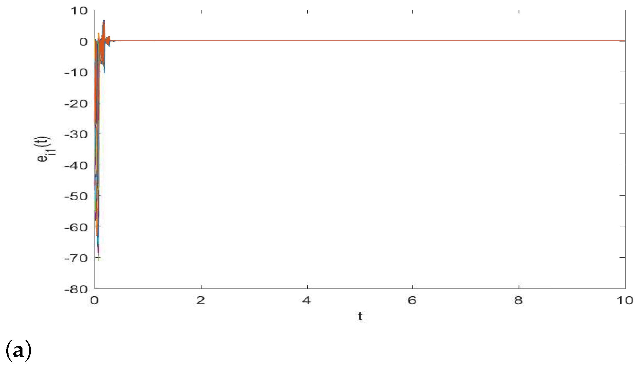
Utilizing the classical Runge-Kutta algorithm, Figure 2 shows the time evolutions of $z_{i1}\left(t\right)$ and $z_{i2}\left(t\right)$ in controlled multi-link complex networks (40) with random initial values. Figure 3 reveals that synchronization error $e_i\left(t\right)$ approaches zero rapidly as the system evolves. It is clear that the synchronization objective of multi-link system (40) can be achieved with a fast convergence under the hybrid impulsive pinning control technology, and the correctness of the theoretical analysis in this paper has been verified.

5. Conclusions

In this article, the mean square synchronization problem of uncertain multi-link stochastic dynamical networks incorporating hybrid time-varying delays has been investigated by pinning and controlling a small number of network nodes. Unlike the existing impulsive control, synchronization impulse and desynchronization impulse are considered at the same time, and the impulse strength and position change with time evolution. Combining coupling matrix decomposition technology and stability theory, some new synchronization criteria, which are bound up with the uncertain strengths, coupling strengths, hybrid impulse strengths, delay sizes, impulsive intervals, and network topologies, are derived to guarantee synchronization for the concerned multi-link model. Ultimately, a simulation experiment shows the rationality of our theory. In the future, we will continue to study how to apply the impulsive pinning control techniques in this article to the corresponding fractional-order multi-link delayed systems. Due to the nonlocality of fractional-order systems and the delay effect, maybe one can establish new fractional-order impulsive comparison principles to overcome this difficulty, which is challenging and meaningful work.

References

1. Shi, K.B.; Wang, J.; Zhong, S.M.; Tang, Y.Y.; Cheng, J. Non-fragile memory filtering of T-S fuzzy delayed neural networks based on switched fuzzy sampled-data control. Fuzzy Sets Syst. 2020, 394, 40–64. [Google Scholar] [CrossRef]
2. Tang, Z.; Park, J.H. Topology and parameters recognition of uncertain complex dynamical via nonidentical adaptive synchronization. Nonlinear Dyn. 2016, 85, 2171–2181. [Google Scholar] [CrossRef]
3. Wei, H.; Zhu, Q.X.; Hamidreza, K. Some improved Razumikhin stability criteria for impulsive stochastic delay differential systems. IEEE Trans. Autom. Control 2019, 64, 5207–5213. [Google Scholar]
4. Wei, H.; Zhu, Q.X. Stability criteria for impulsive stochastic functional differential systems with distributed-delay dependent impulsive effects. IEEE Trans. Syst. Man Cybern. Syst. 2021, 51, 2027–2032. [Google Scholar]
5. Fu, X.Z.; Zhu, Q.X. Stability of nonlinear impulsive stochastic systems with Markovian switching under generalized average dwell time condition. Sci. China Inf. Sci. 2018, 61, 112211. [Google Scholar] [CrossRef]
6. Rao, R.F.; Lin, Z.; Ai, X.Q.; Wu, J.R. Synchronization of epidemic systems with Neumann boundary value under delayed impulse. Mathematics 2022, 10, 2064. [Google Scholar] [CrossRef]
7. Yi, C.B.; Feng, J.W.; Wang, J.Y.; Xu, C.; Zhao, Y. Synchronization of delayed neural networks with hybrid coupling via partial mixed pinning impulsive control. Appl. Math. Comput. 2017, 312, 78–90. [Google Scholar] [CrossRef]
8. Fan, H.G.; Shi, K.B.; Zhao, Y. Pinning impulsive cluster synchronization of uncertain complex dynamical networks with multiple time-varying delays and impulsive effects. Phys. A Stat. Mech. Appl. 2022, 587, 126534. [Google Scholar] [CrossRef]
9. Wang, J.Y.; Feng, J.W.; Xu, C.; Zhao, Y. Cluster synchronization of nonlinearly-coupled complex networks with nonidentical nodes and asymmetrical coupling matrix. Nonlinear Dyn. 2012, 67, 1635–1646. [Google Scholar] [CrossRef]
10. Wang, F.; Zheng, Z.W.; Yang, Y.Q. Quasi-synchronization of heterogenous fractional-order dynamical networks with time-varying delay via distributed impulsive control. Chaos Solitons Fractals 2021, 142, 110465. [Google Scholar] [CrossRef]
11. Wang, F.; Zheng, Z.W. Quasi-projective synchronization of fractional order chaotic systems under input saturation. Phys. A Stat. Mech. Appl. 2019, 534, 122132. [Google Scholar] [CrossRef]
12. Gu, Y.J.; Yu, Y.G.; Wang, H. Projective synchronization for fractional-order memristor-based neural networks with time delays. Neural Comput. Appl. 2019, 31, 6039–6054. [Google Scholar] [CrossRef]
13. Wang, F.; Yang, Y.Q.; Hu, M.F.; Xu, X.Y. Projective cluster synchronization of fractional-order coupled-delay complex network via adaptive pinning control. Phys. A Stat. Mech. Appl. 2015, 434, 134–143. [Google Scholar] [CrossRef]
14. He, W.L.; Cao, J.D. Exponential synchronization of hybrid coupled networks with delayed coupling. IEEE Trans. Neural Netw. 2010, 21, 571–583. [Google Scholar] [PubMed]
15. Li, G.D.; Zhang, Y.; Guan, Y.J.; Li, W.J. Stability analysis of multi-point boundary conditions for fractional differential equation with non-instantaneous integral impulse. Math. Biosci. Eng. 2023, 20, 7020–7041. [Google Scholar] [CrossRef]
16. Cai, S.M.; He, Q.B.; Hao, J.J.; Liu, Z.R. Exponential synchronization of complex networks with nonidentical time-delayed dynamical nodes. Phys. Lett. A 2010, 374, 2539–2550. [Google Scholar] [CrossRef]
17. Zhou, H.; Ma, S.Y.; Li, W.X. Actuator saturating intermittent control for synchronization of stochastic multi-links network with sampled-data. Neurocomputing 2021, 465, 167–183. [Google Scholar] [CrossRef]
18. Guo, Y.; Chen, B.D.; Wu, Y.B. Finite-time synchronization of stochastic multi-links dynamical networks with Markovian switching topologies. J. Frankl. Inst. 2020, 357, 359–384. [Google Scholar] [CrossRef]
19. Xu, Y.; Li, Y.Z.; Li, W.X.; Feng, J.Q. Synchronization of multi-links impulsive fractional-order complex networks via feedback control based on discrete-time state observations. Neurocomputing 2020, 406, 224–233. [Google Scholar] [CrossRef]
20. Sun, Y.Q.; Wu, H.Y.; Chen, Z.H.; Zheng, X.J.; Chen, Y. Outer synchronization of two different multi-links complex networks by chattering-free control. Phys. A Stat. Mech. Appl. 2021, 584, 126354. [Google Scholar] [CrossRef]
21. Qin, X.L.; Wang, C.; Li, L.X.; Peng, H.P.; Yang, Y.X.; Ye, L. Finite-time modified projective synchronization of memristor-based neural network with multi-links and leakage delay. Chaos Solitons Fractals 2018, 116, 302–315. [Google Scholar] [CrossRef]
22. Zhou, L.L.; Tan, F.; Yu, F.; Liu, W. Cluster synchronization of two-layer nonlinearly coupled multiplex networks with multi-links and time-delays. Neurocomputing 2019, 359, 264–275. [Google Scholar] [CrossRef]
23. Zheng, M.W.; Li, L.X.; Peng, H.P.; Xiao, J.H.; Yang, Y.X.; Zhang, Y.P.; Zhao, H. General decay synchronization of complex multi-links time-varying dynamic network. Commun. Nonlinear Sci. Numer. Simul. 2019, 67, 108–123. [Google Scholar] [CrossRef]
24. Li, S.; Li, Y.X.; Ding, X.H. More general results of aperiodically intermittent synchronization for stochastic Markovian switching complex networks with multi-links and time-varying coupling structure. Neurocomputing 2020, 395, 39–55. [Google Scholar] [CrossRef]
25. Wang, P.F.; Li, S.Y.; Su, H. Stabilization of complex-valued stochastic functional differential systems on networks via impulsive control. Chaos Solitons Fractals 2020, 133, 109561. [Google Scholar] [CrossRef]
26. Zhou, H.; Li, W.X. Synchronisation of stochastic-coupled intermittent control systems with delays and Lévy noise on networks without strong connectedness. IET Control Theory Appl. 2019, 13, 36–49. [Google Scholar] [CrossRef]
27. Shi, K.B.; Wang, J.; Zhong, S.M.; Tang, Y.Y.; Cheng, J. Hybrid-driven finite-time H sampling synchronization control for coupling memory complex networks with stochastic cyber attacks. Neurocomputing 2020, 387, 241–254. [Google Scholar] [CrossRef]
28. Zhang, L.; Yang, X.S.; Xu, C.; Feng, J.W. Exponential synchronization of complex-valued complex networks with time-varying delays and stochastic perturbations via time-delayed impulsive control. Appl. Math. Comput. 2017, 306, 22–30. [Google Scholar] [CrossRef]
29. Liu, Y.; Wang, M.; Chu, D.H.; Su, H. Feedback control based on discrete-time state observations on synchronization of stochastic impulsive coupled systems. Nonlinear Anal. Hybrid Syst. 2021, 39, 100987. [Google Scholar] [CrossRef]
30. Zhao, H.; Li, L.X.; Peng, H.P.; Xiao, J.H.; Yang, Y.X. Mean square modified function projective synchronization of uncertain complex network with multi-links and stochastic perturbations. Eur. Phys. J. 2015, 88, 1–8. [Google Scholar] [CrossRef]
31. Tang, Z.; Park, J.H.; Feng, J.W. Novel approaches to pin cluster synchronization on complex dynamical networks in Lur’e forms. Commun. Nonlinear Sci. Numer. Simul. 2018, 57, 422–438. [Google Scholar] [CrossRef]
32. Liang, S.; Wu, R.C.; Chen, L.P. Adaptive pinning synchronization in fractional-order uncertain complex dynamical networks with delay. Phys. A Stat. Mech. Appl. 2016, 444, 49–62. [Google Scholar] [CrossRef]
33. Ding, S.B.; Wang, Z.S. Synchronization of coupled neural networks via an event-dependent intermittent pinning control. IEEE Trans. Syst. Man Cybern. Syst. 2022, 52, 1928–1934. [Google Scholar] [CrossRef]
34. Peng, D.X.; Li, X.D. Leader-following synchronization of complex dynamic networks via event-triggered impulsive control. Neurocomputing 2020, 412, 1–10. [Google Scholar] [CrossRef]
35. Xia, M.L.; Liu, L.N.; Fang, J.Y.; Zhang, Y.C. Stability analysis for a class of stochastic differential equations with impulses. Mathematics 2023, 11, 1541. [Google Scholar] [CrossRef]
36. Tang, Z.; Park, J.H.; Wang, Y.; Feng, J.W. Impulsive synchronization of derivative coupled neural networks with cluster-tree topology. IEEE Trans. Netw. Sci. Eng. 2020, 11, 1541. [Google Scholar] [CrossRef]
37. Fan, H.G.; Shi, K.B.; Zhao, Y. Global μ-synchronization for nonlinear complex networks with unbounded multiple time delays and uncertainties via impulsive control. Phys. A Stat. Mech. Appl. 2022, 599, 127484. [Google Scholar] [CrossRef]
38. Lu, J.Q.; Kurths, J.; Cao, J.D.; Mahdavi, N.; Huang, C. Synchronization control for nonlinear stochastic dynamical networks: Pinning impulsive strategy. IEEE Trans. Neural Netw. Learn. Syst. 2012, 23, 285–292. [Google Scholar]
39. Zhao, Y.Q.; Wang, L.S. Practical exponential stability of impulsive stochastic food chain system with time-varying delays. Mathematics 2023, 11, 147. [Google Scholar] [CrossRef]
40. He, W.L.; Qian, F.; Cao, J.D.; Han, Q.L. Impulsive synchronization of two nonidentical chaotic systems with time-varying delay. Phys. Lett. A 2011, 375, 498–504. [Google Scholar] [CrossRef]
41. Cai, S.M.; Zhou, P.P.; Liu, Z.R. Synchronization analysis of hybrid-coupled delayed dynamical networks with impulsive effects: A unified synchronization criterion. J. Frankl. Inst. 2015, 352, 2065–2089. [Google Scholar] [CrossRef]
42. Yang, Z.C.; Xu, D.Y. Stability analysis and design of impulsive control systems with time delay. IEEE Trans. Autom. Control 2007, 52, 1448–1454. [Google Scholar] [CrossRef]
Figure 1. (A) Complete transportation network; (A1) aviation network; (A2) land network; and (A3) waterway network.
Mathematics 11 01697 g001
Figure 2. Time evolution of z i ( t ) in multi-link complex networks (40) under the hybrid impulsive pinning control. (a) z i 1 ( t ) ; (b) z i 2 ( t ) .
Mathematics 11 01697 g002
Figure 3. The state of synchronization errors in multi-link complex networks (40) under the hybrid impulsive pinning control. (a) e i 1 ( t ) ; (b) e i 2 ( t ) .
Mathematics 11 01697 g003aMathematics 11 01697 g003b
Disclaimer/Publisher’s Note: The statements, opinions and data contained in all publications are solely those of the individual author(s) and contributor(s) and not of MDPI and/or the editor(s). MDPI and/or the editor(s) disclaim responsibility for any injury to people or property resulting from any ideas, methods, instructions or products referred to in the content.