Stability Analysis for a Class of Stochastic Differential Equations with Impulses

Abstract

This paper is concerned with the problem of asymptotic stability for a class of stochastic differential equations with impulsive effects. A sufficient criterion on asymptotic stability is derived for such impulsive stochastic differential equations via Lyapunov stability theory, bounded difference condition and martingale convergence theorem. The results show that the impulses can facilitate the stability of the stochastic differential equations when the original system is not stable. Finally, the feasibility of our results is confirmed by two numerical examples and their simulations.

1. Introduction

It is well known that stability is the essential condition to maintain the normal operation of dynamic systems, so stability analysis of systems has made long-term developmen [1,2,3,4,5]. During the evolution of dynamic systems, the state of the system changes abruptly at certain moments, and such systems are called impulsive systems. Impulsive systems are extensively researched in the fields of biology, economy, communication, and power systems, as they can perform both continuous and discrete dynamical behaviors. Therefore, impulsive differential equations are applied as mathematical models for many physical phenomena. In fact, the impulses are divided into stabilizing impulses and perturbed impulses, and the discrete dynamics behavior can be activated frequently by stabilizing impulses to suppress the unstable continuous behavior [6,7,8,9,10,11,12,13]. For example, ref. [7] utilizes the indefinite Lyapunov function and the impulse controller to obtain the conditions on asymptotic stability of solution for the impulsive systems. In [10], the exponential stability is investigated by employing impulsive control theory and several analytical techniques for nonlinear time-delay impulsive control systems. Literature [12] researches asymptotic stability conditions of impulsive differential systems based on comparison principle and vectorial Lyapunov functions. Therefore, it has significant and practical importance to analyze the effect of impulses on the stability of systems.

Stochastic disturbances commonly exist in the real life. For example, environmental noise, accidental emergencies, etc., and sometimes such stochastic factors may change the state of the original dynamic systems. Therefore, stochastic differential equations are introduced to characterize such dynamical systems with disturbances of stochastic factors [14,15,16,17,18,19]. Due to the potential presence of both impulse effects and stochastic factors, dynamic systems are often modeled as impulsive stochastic differential equations. It is noteworthy that many scholars are devoted to exploring the role of impulses in stabilizing unstable systems [20,21,22,23,24,25]. For example, in [20], the pth moment exponential stability is investigated on the basis of vector Lyapunov function and Razumikhin technique for impulsive time-delay stochastic differential systems. In [21], the exponential stability is developed by utilizing stochastic analysis techniques, the Razumikhin approach and average impulsive delay condition for stochastic delayed differential systems with average-delay impulses. In [24], the almost sure exponential stability of a class of nonlinear stochastic differential systems with impulse is established based on the Lyapunov function.

To date, the existing literature has analyzed the stability of the system by utilizing some classical methods for impulsive stochastic differential equations. For instance, the comparison method [26,27] and the average dwell time method [28,29,30,31]. Literature [26] obtains conditions for asymptotic stability of solution for time-varying impulsive differential equations through the Lyapunov function, comparison principle and some inequalities. However, it may be difficult to construct suitable comparison systems for real systems, which makes the theoretical results more conservative. Ref. [30] establishes sufficient conditions for the global stability of impulsive stochastic systems by using Lyapunov stability theory and the average dwell time condition. Yet there are two aspects we should pay attention to. On the one hand, it is generally hard to test the average dwell time condition in advance. On the other hand, the average dwell time condition does not ensure the tightness or sparsity of the impulse jumps. According to the above discussion, the asymptotic stability criterion on stochastic differential equations with impulsive effects is established in this paper based on Lyapunov stability theory, bounded difference condition and martingale convergence theorem as well as some lemmas and inequality techniques. It is interesting that the bounded difference method is more effective in ensuring the stability of impulsive stochastic differential equations. As far as the authors know, this method is not used in the existing literature in the analysis of stability for stochastic differential equations with stabilizing impulses.

This paper is described below. In Section 2, we will introduce the model and some descriptions. In Section 3, sufficient conditions are given about the asymptotic stability of impulsive stochastic differential equations. Two examples and their simulations illustrate the feasibility of the theoretical results in Section 4. Section 5 draws a conclusion.

2. Preliminaries

Let $(\Omega ,\mathcal{F},P)$ stand for a complete probability space with a filtration ${\left\{{\mathcal{F}}_t\right\}}_{t\ge 0}$ satisfying the usual conditions, i.e., it is right continuous and ${\mathcal{F}}_0$ contains all $\mathbb{P}$-null sets. Let $\omega \left(t\right)={({\omega }_1\left(t\right),\dots ,{\omega }_n\left(t\right))}^{\top }$ be n-dimensional Brownian motion in this space. Given that $\mathbb{N}$ means all positive integers. $\mathbb{R}$ represent all real numbers, ${\mathbb{R}}^{+}$ is a nonnegative member in set $\mathbb{R}$, that is, ${\mathbb{R}}^{+}=[0,+\infty )$, ${\mathbb{R}}^n$ and ${\mathbb{R}}^{n\times n}$ be the n-dimensional vectors and $n\times n$ real matrices, respectively. A vector or matrix Y with transpose is defined as $Y^{\top }$. $\mathbb{E}[·]$ means the mathematical expectation. For $y\in {\mathbb{R}}^n$, $\left|y\right|$ represents the Euclidean vector norm. $Y<0(Y>0)$ means negative (positive) of matrix Y.

Firstly, we will consider the stochastic differential equations

$$dy\left(t\right)=Ey\left(t\right)dt+Fy\left(t\right)d\omega \left(t\right),t\in \left[t_{k-1},t_k\right),$$

(1)

where the state $y\left(t\right)\in {\mathbb{R}}^n$, the initial value $y\left(t_0\right)=y_0$, E and F are constant mataices.

Next, consider stochastic differential equations with impulsive effects as follows,

$$\left\{\begin{array}{cc}\hfill & dy\left(t\right)=Ey\left(t\right)dt+Fy\left(t\right)d\omega \left(t\right),t\in \left[t_{k-1},t_k\right),\hfill \\ \hfill & y\left({t_k}^{+}\right)-y\left({t_k}^{-}\right)=b_{k}y\left({t_k}^{-}\right),t=t_k,k\in \mathbb{N},\hfill \end{array}\right.$$

(2)

where $y\left(t\right)$ is right-continuous at $t_k$, namely $y\left(t_k\right)=y\left({t_k}^{+}\right)$, ${\left\{t_k\right\}}_{k=1}^{\infty }$ is the impulsive jump point and $b_k\in \left(-2,0\right)$.

Hencel system (2) is equivalent to

$$\left\{\begin{array}{cc}\hfill & dy\left(t\right)=Ey\left(t\right)dt+Fy\left(t\right)d\omega \left(t\right),t\in \left[t_{k-1},t_k\right),\hfill \\ \hfill & y\left(t_k\right)={\mu }_{k}y\left({t_k}^{-}\right),t=t_k,k\in \mathbb{N},\hfill \end{array}\right.$$

(3)

where ${\mu }_k=1+b_k$ satisfying $|{\mu }_k|\in \left(0,1\right).$

In this paper, $h_k$ is defined as the length of impulse interval on the range $\left[t_{k-1,}{t}_k\right)$, namely $h_k=t_k-t_{k-1}$. We suppose that ${\left\{h_k\right\}}_{k\in \mathbb{N}}$ are uniformly bounded, i.e., it has a positive number h which satisfies $h_k\le h$. Furthermore the impulsive interval lengths $h_1$, $h_2$, …, are independent random variables on the probability space $(\Omega ,\mathcal{F},P)$.

It is necessary to introduce several definitions and lemmas before getting the condition of stability for systems (3).

Definition 1.

The solution $y\left(t\right)$ of Equation (3) is said to be mean square asymptotically stable

$$\underset{t\to \infty }{lim}\mathbb{E}|y\left(t\right){|}^2=0,$$

for any initial value $y_0\in {\mathbb{R}}^n$.

Definition 2.

If there exists a positive number L satisfying

$$\left|l_{k+1}-l_k\right|\le L,$$

then for $\forall k\in \mathbb{N}$, ${\left\{l_k\right\}}_{k\in \mathbb{N}}$ is called bounded difference sequence.

Remark 1.

Both the literature [32] and this paper utilize bounded difference conditions to research the stability of the system, yet they are completely different. On the one hand, the model is changed from ordinary differential equations to stochastic differential equations, and on the other hand, the impulse type is changed from perturbed impulses to stabilizing impulses.

Definition 3.

Give a function $V\left(x\left(t\right)\right):{\mathbb{R}}^n\to {\mathbb{R}}^{+}$, an operator $\mathcal{L}V\left(x\right(t\left)\right)$ is defined by

$$\mathcal{L}V\left(y\left(t\right)\right)=V_t\left(y\left(t\right)\right)+V_y\left(y\left(t\right)\right)f\left(y\left(t\right)\right)+\frac{1}{2}trace\left[g{\left(y\left(t\right)\right)}^T{V}_{yy}g\left(y\left(t\right)\right)\right].$$

$$\begin{array}{cc}\hfill & V_t\left(y\left(t\right)\right)=\frac{\partial V\left(y\right(t\left)\right)}{\partial t},V_y\left(y\left(t\right)\right)=\left(\frac{\partial V\left(y\right(t\left)\right)}{\partial y_1},\dots ,\frac{\partial V\left(y\right(t\left)\right)}{\partial y_n}\right),\hfill \\ \hfill & V_{yy}\left(y\left(t\right)\right)={\left(\frac{{\partial }^{2}V\left(y\left(t\right)\right)}{\partial y_i\partial y_j}\right)}_{n\times n}.\hfill \end{array}$$

Definition 4.

If the random variable ${\left\{Y_n\right\}}_{n\ge 0}$ is integrable and satisfies inequality $\mathbb{E}\left(Y_{n+1}|{\mathcal{F}}_n\right)\le Y_n$, then ${\left\{Y_n\right\}}_{n\ge 0}$ is denoted by nonnegative super-martingale, with respect to natural filtration ${\left\{{\mathcal{F}}_n\right\}}_{n\ge 0}$.

Definition 5

(Martingale convergence theorem). For nonnegative super-martingale ${\left\{Y_n\right\}}_{n\ge 0}$, if $sup\mathbb{E}\left|Y_n\right|<+\infty$, then ${\left\{Y_n\right\}}_{n\ge 0}$ converges to the integrable random variable $Y_{\infty }$ as $n\to \infty$ and $\mathbb{E}\left(Y_{\infty }|{\mathcal{F}}_n\right)\le Y_n$.

Lemma 1

(Gronwall inequality). Supposed that $u(·)$, $v(·)$ and $a(·)$ be real-valued continuous functions, satisfing

$$a\left(t\right)\le u\left(t\right)+{\int }_0^{t}v\left(s\right)a\left(s\right)ds,$$

for $\forall t\ge 0$, then

$$a\left(t\right)\le u\left(t\right){\mathrm{e}}^{{\int }_0^{t}v\left(s\right)\mathrm{d}s}.$$

Lemma 2

(Fatou’s lemma). Let ${\left\{g_k\right\}}_{k\in \mathbb{N}}$ be a sequence of non-negative random variables on some probability space then

$$\mathbb{E}\left[\underset{n\to \infty }{lim}inf{g}_n\right]\le \underset{n\to \infty }{lim}inf\mathbb{E}\left[g_n\right].$$

Lemma 3

(see [33] Schur complement). Assume that $P_1$, $P_3$ are matrices of appropriate dimensions, $P_2$ is a positive definite matrix, then the following two equations are equivalent,

(1) 

$P_2<0,P_1-P_3{P}_2^{-1}{P}_3^{\top }<0$,

(2) 

$\left[\begin{array}{cc}{P}_1& P_3\\ P_3^{\top }& P_2\end{array}\right]<0$.

3. Main Results

Next, we will establish the stability criterion for stochastic differential equations with impulses by Lyapunov stability theory, bounded difference condition and martingale convergence theorem.

Theorem 1.

The solution of stochastic system (3) is asymptotic stable if there exist a positive number η, a positive definite matrix R and bounded differences subsequence ${\left\{l_k\right\}}_{k\in \mathbb{N}}$ such that

(1)

$$RE+E^{\top }R+F^{\top }RF-\eta R<0,$$

(4)

(2)

$$\underset{j\to \infty }{lim}\left\{\prod _{k=1}^{l_j}{\left({\mu }_k\right)}^2\right\}=0.$$

(5)

Proof. 

Construct a Lyapunov function

$$V\left(y\left(t\right)\right)=y^T\left(t\right)Ry\left(t\right),$$

thus, we know that

$${\lambda }_1{\left(R\right)\left|y\left(t\right)\right|}^2\le V\left(y\left(t\right)\right)\le {\lambda }_2\left(R\right){\left|y\left(t\right)\right|}^2,$$

where ${\lambda }_1\left(R\right)$ and ${\lambda }_2\left(R\right)$ are minimum and maximum eigenvalue of positive definite matrix R respectively. □

It is derived from (3), for $t\in [t_{k-1},t_k)$

$$y\left(t\right)=y\left(t_{k-1}\right)+\underset{t_{k-1}}{\overset{t}{\int }}Ey\left(s\right)ds+\underset{t_{k-1}}{\overset{t}{\int }}Fy\left(s\right)d\omega \left(s\right).$$

In view of elementary inequality and Hölder inequality, one gets

$$\begin{array}{cc}\hfill {\left|y\left(t\right)\right|}^2\le & 3{\left|y\left(t_{k-1}\right)\right|}^2+3\left(t-t_{k-1}\right){\int }_{t_{k-1}}^t{\left|Ey\left(s\right)\right|}^{2}ds\hfill \\ \hfill & +3{\left|{\int }_{t_{k-1}}^{t}Fy\left(s\right)d\omega \left(s\right)\right|}^2.\hfill \end{array}$$

(6)

Taking the expectation of inequality (6) on both sides,

$$\begin{array}{cc}\hfill {\mathbb{E}\left|y\left(t\right)\right|}^2\le & 3\mathbb{E}{\left|y\left(t_{k-1}\right)\right|}^2+{3\left|E\right|}^2\left(t-t_{k-1}\right){\int }_{t_{k-1}}^t\mathbb{E}{\left|y\left(s\right)\right|}^{2}ds\hfill \\ \hfill & +3\mathbb{E}{\left|{\int }_{t_{k-1}}^{t}Fy\left(s\right)d\omega \left(s\right)\right|}^2\hfill \\ \hfill \le & 3\mathbb{E}{\left|y\left(t_{k-1}\right)\right|}^2+{3\left|E\right|}^2\left(t-t_{k-1}\right){\int }_{k_{k-1}}^t\mathbb{E}{\left|y\left(s\right)\right|}^{2}ds\hfill \\ \hfill & +3\mathbb{E}{\int }_{t_{k-1}}^t{\left|Fy\left(s\right)\right|}^{2}ds\hfill \\ \hfill \le & 3\mathbb{E}{\left|y\left(t_{k-1}\right)\right|}^2+3\left({\left|E\right|}^2\left(t-t_{k-1}\right)+{\left|F\right|}^2\right){\int }_{t_{k-1}}^t\mathbb{E}{\left|y\left(s\right)\right|}^{2}ds.\hfill \end{array}$$

By the Lemma 1, the following inequation holds

$${\mathbb{E}\left|y\left(t\right)\right|}^2⩽3\mathbb{E}{\left|y\left(t_{k-1}\right)\right|}^2{e}^{3\left(t-t_{k-1}\right)\left({\left|E\right|}^2\left(t-t_{k-1}\right)+{\left|F\right|}^2\right)}.$$

(7)

It follows from Itô’s formula that

$$\begin{array}{c}dV\left(y\left(t\right)\right)=\mathcal{L}V\left(y\left(t\right)\right)dt+V_x\left(y\left(t\right)\right)\left(Fy\left(t\right)\right)d\omega \left(t\right).\hfill \end{array}$$

(8)

Here $\delta >0$ is small enough to satisfy $t+\delta \in \left(t_{k-1},t_k\right)$, one has

$$\mathbb{E}V\left(y(t+\delta )\right)-\mathbb{E}V\left(y\left(t\right)\right)={\int }_t^{t+\delta }\mathbb{E}\mathcal{L}V\left(y\left(s\right)\right)ds.$$

Thus

$$\begin{array}{cc}\hfill D^{+}\mathbb{E}V\left(y\left(t\right)\right)& =\mathbb{E}\mathcal{L}V\left(y\right(t\left)\right)\hfill \\ \hfill & =\mathbb{E}\left[2y^{\top }\left(t\right)REy\left(t\right)+{\left(Fy\left(t\right)\right)}^{\top }R\left(Fy\left(t\right)\right)\right]\hfill \\ \hfill & =\mathbb{E}\left[y^{\top }\left(t\right)\left(2RE+F^{\top }RF-\eta R\right)y\left(t\right)+y^{\top }\left(t\right)\left(\eta R\right)y\left(t\right)\right].\hfill \end{array}$$

(9)

By condition (4), we can see

$$D^{+}\mathbb{E}V\left(y\right(t\left)\right)\le \mathbb{E}\left[y^{\top }\left(t\right)\left(\eta R\right)y\left(t\right)\right]=\eta \mathbb{E}V\left(y\right(t\left)\right),$$

(10)

then (10) can be solved as

$$\mathbb{E}V\left(y\right(t\left)\right)\le \mathbb{E}\left[V\left(y\left(t_{k-1}\right)\right)e^{\eta (t-t_{k-1})}\right],$$

for $t\in \left[t_{k-1},t_k\right)$.

Therefore, the results show that

$$\mathbb{E}V\left(y\left(t_k^{-}\right)\right)\le \mathbb{E}\left[V\left(y\left(t_{k-1}\right)\right)e^{\eta ({t_k}^{-}-t_{k-1})}\right].$$

(11)

It is obtained from (3) and (11)

$$\begin{array}{cc}\hfill \mathbb{E}V\left(y\left(t_k\right)\right)& =\mathbb{E}\left[y^{\top }\left(t_k\right)Ry\left(t_k\right)\right]\hfill \\ \hfill & ={\left({\mu }_k\right)}^2\mathbb{E}\left[y^{\top }\left(t_k{}^{-}\right)Ry\left(t_k{}^{-}\right)\right]\hfill \\ \hfill & ={\left({\mu }_k\right)}^2\mathbb{E}V\left(y\left(t_k{}^{-}\right)\right)\hfill \\ \hfill & \le {\left({\mu }_k\right)}^2{e}^{\eta h_k}\mathbb{E}V\left(y\left(t_{k-1}\right)\right).\hfill \end{array}$$

(12)

Since $h_k$ is uniformly bounded, $e^{\eta h_k}$ is integrable and it is obvious from Equation (12) that $V\left(y\left(t_k\right)\right)$ is integrable, which shows that

$$\begin{array}{cc}\hfill \mathbb{E}\left[V\left(y\left(t_k\right)\right)|{\mathcal{F}}_{k-1}\right]& \le {\left({\mu }_k\right)}^2{e}^{\eta h_k}\mathbb{E}\left[V\left(y\left(t_{k-1}\right)\right)|{\mathcal{F}}_{k-1}\right]\hfill \\ \hfill & \le {\left({\mu }_k\right)}^2{e}^{\eta h_k}V\left(y\left(t_{k-1}\right)\right).\hfill \end{array}$$

(13)

Based on uniform boundedness of $h_k$, nonnegative super-martingale ${\left\{V\left(y\left(t_{l_j}\right)\right)\right\}}_{j\in \mathbb{N}}$ and (5), we get that ${\left\{V\left(y\left(t_{l_j}\right)\right)\right\}}_{j\in \mathbb{N}}$ converges to a non-negative random variable $V_{\infty }$ from martingale convergence theorem.

In view of $\mathbb{E}\left\{V\left(y\left(t_k\right)\right)\right\}=\mathbb{E}\left[\mathbb{E}\left[V\left(y\left(t_k\right)\right)|{\mathcal{F}}_{k-1}\right]\right]$, we have

$$\mathbb{E}\left\{V\left(y\left(t_{l_j}\right)\right)\right\}\le \left\{{\prod }_{k=1}^{l_j}{\left({\mu }_k\right)}^2\right\}{e}^{\eta h}\mathbb{E}\left\{V\left(y\left(t_0\right)\right)\right\}.$$

(14)

According to the Lemma 2, there holds

$$\begin{array}{cc}\hfill \mathbb{E}\left\{V_{\infty }\right\}& =\mathbb{E}\left[\underset{j\to \infty }{lim}V\left(y\left(t_{l_j}\right)\right)\right]\hfill \\ & =\mathbb{E}\left[\underset{j\to \infty }{lim}infV\left(y\left(t_{l_j}\right)\right)\right]\hfill \\ & \le \underset{j\to \infty }{lim}inf\mathbb{E}\left[V\left(y\left(t_{l_j}\right)\right)\right]\hfill \\ & \le \underset{j\to \infty }{lim}\left\{\prod _{k=1}^{l_j}{\left({\mu }_k\right)}^2\right\}{e}^{\eta h}\mathbb{E}\left\{V\left(y\left(t_0\right)\right)\right\}.\hfill \end{array}$$

From condition (5), it is obtain that $\mathbb{E}\left\{V_{\infty }\right\}=0$. It is obvious that the sequence ${\left\{V\left(y\left(t_{l_j}\right)\right)\right\}}_{j\in \mathbb{N}}$ converges to zero.

It follows from (7) that

$$\begin{array}{cc}\hfill {\mathbb{E}\left|y\left(t\right)\right|}^2& \le 3\mathbb{E}{\left|y\left(t_{k-1}\right)\right|}^2{e}^{3\left(t-t_{k-1}\right)\left({\left|E\right|}^2\left(t-t_{k-1}\right)+{\left|F\right|}^2\right)}\hfill \\ \hfill & \le 3^{\left(k-l_{j-1}\right)}M{e}^{{\gamma }_k}\cdots e^{{\gamma }_{l_{j-1}+1}}\mathbb{E}{\left|y\left(t_{l_{j-1}}\right)\right|}^2,\hfill \end{array}$$

(15)

for $t\in \left[t_{k-1,}{t}_k\right]\subset \left[t_{l_{j-1}},t_{l_j}\right]$, where $M=|{\mu }_{k-1}{|}^2\dots {\left|{\mu }_{l_{j-1}+1}\right|}^2$, ${\gamma }_k=3h_k\left({\left|E\right|}^2{h}_k+{\left|F\right|}^2\right)$.

On the basis of uniform boundedness of $h_k$ and bounded difference condition ${\left\{l_k\right\}}_{k\in \mathbb{N}}$, the following inequalities hold

$$\begin{array}{c}{\mathbb{E}\left|y\left(t\right)\right|}^2\hfill \\ \le 3^{\left(k-l_{j-1}\right)}M{e}^{{\gamma }_k}\cdots e^{{\gamma }_{l_{j-1}+1}}\mathbb{E}{\left|y\left(t_{l_{j-1}}\right)\right|}^2\hfill \\ \le 3^{\left(k-l_{j-1}\right)}M{e}^{3hL\left({\left|E\right|}^{2}h+{\left|F\right|}^2\right)}\mathbb{E}{\left|y\left(t_{l_{j-1}}\right)\right|}^2\hfill \\ \le \frac{3^{\left(k-l_{j-1}\right)}M}{{\lambda }_1\left(R\right)}{e}^{3hL\left({\left|E\right|}^{2}h+{\left|F\right|}^2\right)}\mathbb{E}\left[V\left(y\left(t_{l_j}\right)\right)\right].\hfill \end{array}$$

Therefore, $\underset{t\to \infty }{lim}\mathbb{E}|y\left(t\right){|}^2=0$.

Remark 2.

From Lemma 3, in Theorem 1 the condition (4) is equals to

$$\left(\begin{array}{cc}RE+E^{\top }R-\eta R& F^{\top }\\ & -R^{-1}\end{array}\right)<0.$$

(16)

It is easy to solve the positive definite matrix R by using Matlab LMI toolbox.

4. Numerical Simulations

As a result of the above theoretical derivation of stability for system (3), two numerical examples are provided in this section that illustrate the feasibility of our results.

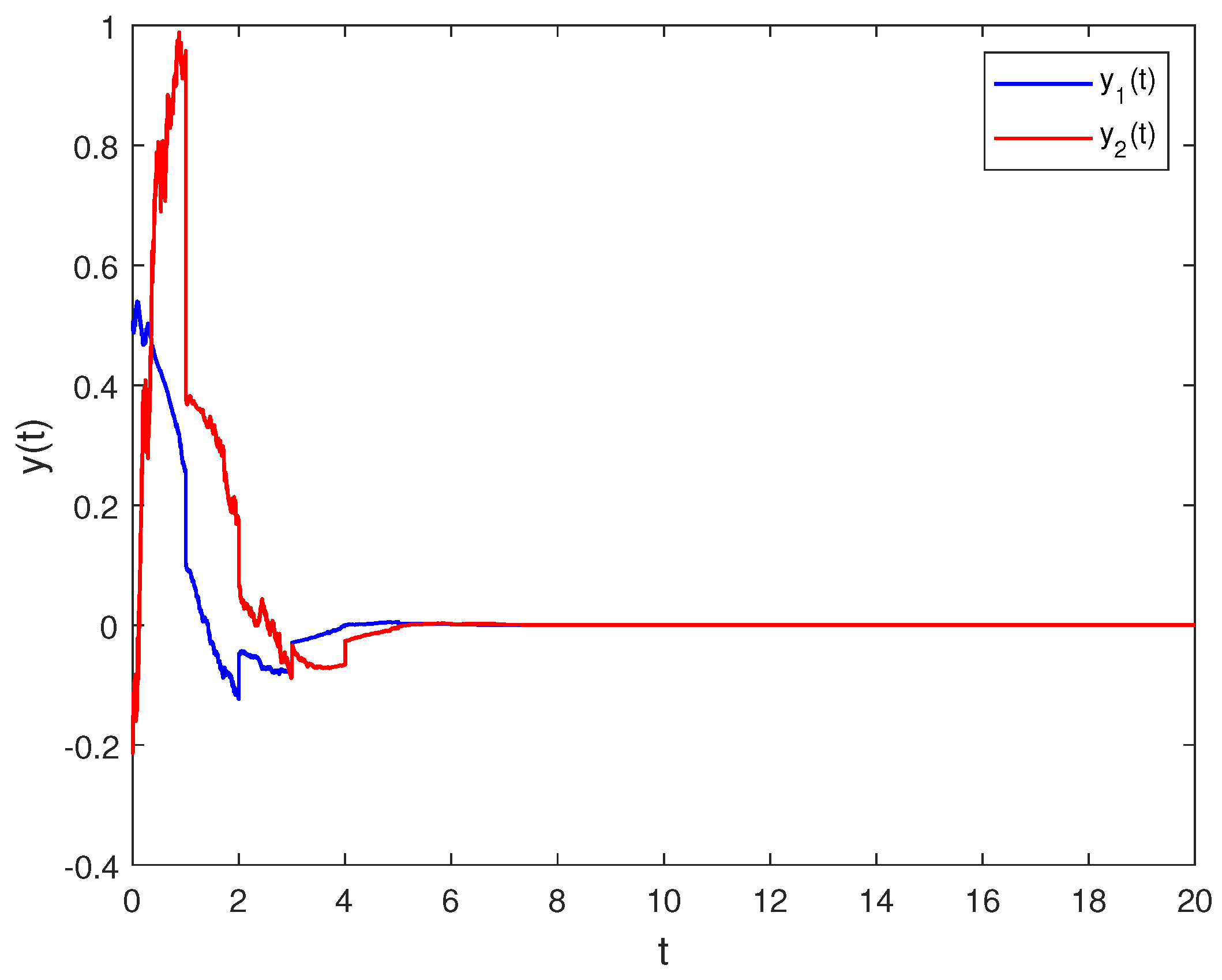
Example 1.

Firstly, we consider the two-dimensional stochastic differential equations with impulsive effects,

$$\left\{\begin{array}{c}dy\left(t\right)=\left(\begin{array}{cc}0.3& -0.5\\ 3& -0.6\end{array}\right)y\left(t\right)dt+\left(\begin{array}{cc}0.2& -0.1\\ -0.8& 0.1\end{array}\right)y\left(t\right)dw\left(t\right),t\in \left[t_{k-1},t_k\right),\hfill \\ y\left(t_k\right)=0.4y\left(t_k^{-}\right),t=t_k,k\in \mathbb{N},\hfill \end{array}\right.$$

(17)

where state $y\left(t\right)\in {\mathbb{R}}^2$.

We choose $\eta =3$, the feasible solution of LMI (16) is derived by Matlab toolbox

$$R=\left[\begin{array}{cc}32.5001& 5.4141\\ 5.4141& 11.3585\end{array}\right].$$

Therefore, it is clear from Theorem 1 that stochastic systems (17) is asymptotically stable.

The simulation results are as follows. For the initial condition $y{}_0={(0.5,-0.2)}^T$, in Figure 1, the state is unstable for stochastic systems (17) without stabilizing impulses. According to Figure 2 one can see that the state is stable for stochastic systems (17) with stabilizing impulses. We can derive that the impulses contribute to the stability of the system state.

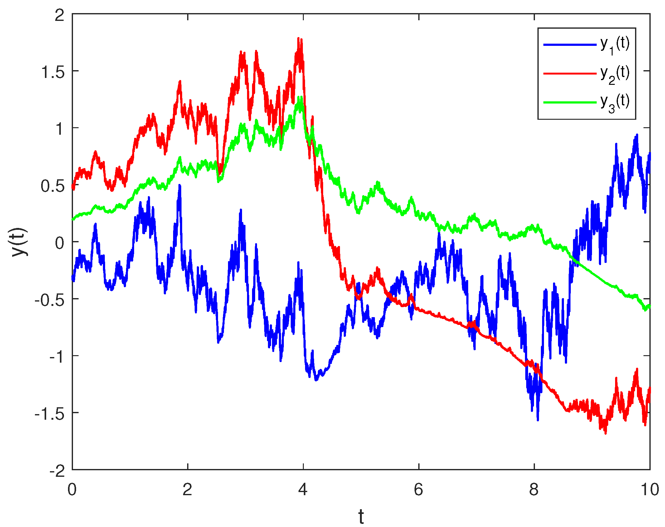
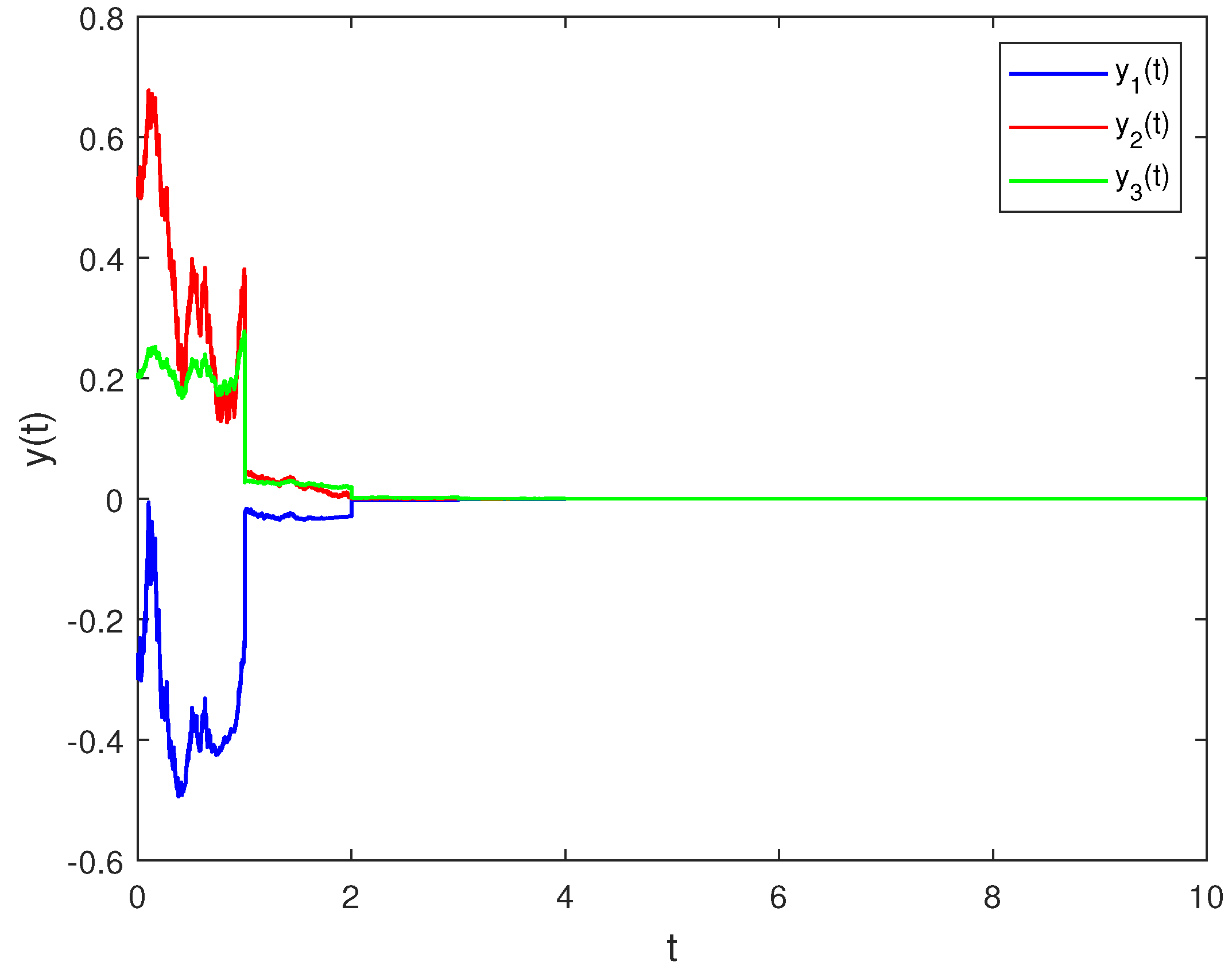
Example 2.

Next, we investigate the following three-dimensional impulsive stochastic differential equation,

$$\left\{\begin{array}{c}dy\left(t\right)=\left(\begin{array}{ccc}-1& 0.2& -0.5\\ 0.3& 0.1& 0.4\\ 0& 0.2& 0.1\end{array}\right)y\left(t\right)dt+\left(\begin{array}{ccc}-0.2& -0.8& 0\\ 0.3& -0.2& -0.4\\ 0& 0.1& -0.5\end{array}\right)y\left(t\right)dw\left(t\right),t\in \left[t_{k-1},t_k\right),\hfill \\ y\left(t_k\right)=0.1y\left(t_k^{-}\right),t=t_k,k\in \mathbb{N},\hfill \end{array}\right.$$

(18)

where state $y\left(t\right)\in {\mathbb{R}}^3$.

We set $\eta =6$, by solving LMI (16) in Remark 2, the feasible solution is obtained as follows

$$R=\left[\begin{array}{ccc}3.2678& 0.3266& -0.2426\\ 0.3266& 4.7449& 0.5246\\ -0.2426& 0.5246& 4.7890\end{array}\right].$$

For the initial value $y{}_0={(-0.3,0.5,0.2)}^T$, Figure 3 and Figure 4 indicate that the solution of system (18) with stabilizing impulses is asymptotically stable. As we observe, the convergence time of the state trajectory is shorter for the system (18) with impulsive effects.

5. Conclusions

Based on Lyapunov stability theory, bounded difference condition and martingale convergence theorem, the stability condition is derived for stochastic differential equations with stabilizing impulses. Finally, two examples and simulation figures are given to demonstrate the efficiency of the stability condition. Furthermore, the results of this paper will be applied to the stability analysis of nonlinear impulsive stochastic differential equations and stochastic homogeneous differential equations .

References

- Chen, C. Explicit solutions and stability properties of homogeneous polynomial dynamical systems via tensor orthogonal decomposition. arXiv 2021, arXiv:2107.11438. [Google Scholar]
- Liu, X.; Shen, J. Stability theory of hybrid dynamical systems with time delay. IEEE Trans. Autom. Control 2006, 51, 620–625. [Google Scholar] [CrossRef]
- Haddad, W.M.; L’Afflitto, A. Finite-time stabilization and optimal feedback control. IEEE Trans. Autom. Contro. 2016, 61, 1069–1074. [Google Scholar] [CrossRef]
- Ahmadi, A.A.; Khadir, B.E. On algebraic proofs of stability for homogeneous vector fields. IEEE Trans. Autom. Control 2019, 65, 325–332. [Google Scholar] [CrossRef] [Green Version]
- Jungers, R.; Ahmadi, A.A.; Parrilo, P.A.; Roozbehani, M. A characterization of Lyapunov inequalities for stability of switched systems. IEEE Trans. Autom. Control 2017, 62, 3062–3067. [Google Scholar] [CrossRef] [Green Version]
- Liu, B.; Xu, B.; Zhang, G.; Tong, L. Review of some control theory results on uniform stability of impulsive systems. Mathematics 2019, 7, 1186. [Google Scholar] [CrossRef] [Green Version]
- Li, H.; Liu, A. Asymptotic stability analysis via indefinite Lyapunov functions and design of nonlinear impulsive control systems. Nonlinear Anal. Hybrid Syst. 2020, 38, 100936. [Google Scholar] [CrossRef]
- Rao, R.; Lin, Z.; Ai, X.; Wu, J. Synchronization of epidemic systems with Neumann boundary value under delayed impulse. Mathematics 2022, 10, 2064. [Google Scholar] [CrossRef]
- Li, X.; Li, P. Stability of time-delay systems with impulsive control involving stabilizing delays. Automatica 2020, 124, 109336. [Google Scholar] [CrossRef]
- Li, X.; Cao, J.; Ho, D.W.C. Impulsive control of nonlinear systems with time-varying delay and applications. IEEE Trans. Cybern. 2020, 50, 2661–2673. [Google Scholar] [CrossRef]
- Jiang, B.; Lu, J.; Liu, Y. Exponential stability of delayed systems with average-delay impulses. SIAM J. Control Optim. 2020, 58, 3763–3784. [Google Scholar] [CrossRef]
- Ai, Z.; Chen, C. Asymptotic stability analysis and design of nonlinear impulsive control systems. Nonlinear Anal. Hybrid Syst. Int. Multidiscip. J. 2017, 24, 244–252. [Google Scholar] [CrossRef]
- Li, G.; Zhang, Y.; Guan, Y.; Li, W. Stability analysis of multi-point boundary conditions for fractional differential equation with non-instantaneous integral impulse. Math. Biosci. Eng. 2023, 20, 7020–7041. [Google Scholar] [CrossRef]
- Mao, X. Stochastic Differential Equations and Applications; Elsevier: Amsterdam, The Netherlands, 2007. [Google Scholar]
- Calvin, T.; Rostand, N. Impact of financial crisis on economic growth: A stochastic model. Stoch. Qual. Control 2022, 37, 45–63. [Google Scholar]
- Jin, X.; Li, Y.X. Adaptive fuzzy control of uncertain stochastic nonlinear systems with full state constraints. Inf. Sci. 2021, 574, 625–639. [Google Scholar] [CrossRef]
- Yu, J.; Yu, S.; Yan, Y. Fixed-time stability of stochastic nonlinear systems and its application into stochastic multi-agent systems. IET Control Theory Appl. 2021, 15, 126–135. [Google Scholar] [CrossRef]
- Liu, J.; Wu, L.; Wu, C.; Luo, W.; Franquelo, L.G. Event-triggering dissipative control of switched stochastic systems via sliding mode. Automatica 2019, 103, 261–273. [Google Scholar] [CrossRef]
- Zhu, Q.; Kong, F.; Cai, Z. Special issue “advanced symmetry methods for dynamics, control, optimization and applications”. Symmetry 2022, 15, 26. [Google Scholar] [CrossRef]
- Cao, W.; Zhu, Q. Razumikhin-type theorem for p th exponential stability of impulsive stochastic functional differential equations based on vector Lyapunov function. Nonlinear Anal. Hybrid Syst. 2021, 39, 100983. [Google Scholar] [CrossRef]
- Xu, H.; Zhu, Q. New criteria on p th moment exponential stability of stochastic delayed differential systems subject to average-delay impulses. Syst. Control Lett. 2022, 164, 105234. [Google Scholar] [CrossRef]
- Hu, W.; Zhu, Q. Stability criteria for impulsive stochastic functional differential systems with distributed-delay dependent impulsive effects. IEEE Trans. Syst. Man Cybern. Syst. 2019, 51, 2027–2032. [Google Scholar] [CrossRef]
- Hu, Z.; Mu, X. Event-triggered impulsive control for nonlinear stochastic systems. IEEE Trans. Cybern. 2021, 52, 7805–7813. [Google Scholar] [CrossRef]
- Cheng, P.; Deng, F.; Yao, F. Almost sure exponential stability and stochastic stabilization of stochastic differential systems with impulsive effects. Nonlinear Anal. Hybrid Syst. 2018, 30, 106–117. [Google Scholar] [CrossRef]
- Zhao, Y.; Wang, L. Practical exponential stability of impulsive stochastic food chain system with time-varying delays. Mathematics 2023, 11, 147. [Google Scholar] [CrossRef]
- He, Z.; Li, C.; Cao, Z.; Li, H. Stability of nonlinear variable-time impulsive differential systems with delayed impulses. Nonlinear Anal. Hybrid Syst. 2021, 39, 100970. [Google Scholar] [CrossRef]
- Wang, Y.; Lu, J. Some recent results of analysis and control for impulsive systems. Commun. Nonlinear Sci. Numer. Simul. 2020, 80, 104862.1–104862.15. [Google Scholar] [CrossRef]
- Li, X.; Song, S.; Wu, J. Exponential stability of nonlinear systems with delayed impulses and applications. IEEE Trans. Autom. Control 2019, 64, 4024–4034. [Google Scholar] [CrossRef]
- Cao, W.; Zhu, Q. Stability of stochastic nonlinear delay systems with delayed impulses. Appl. Math. Comput. 2022, 421, 126950. [Google Scholar] [CrossRef]
- Ren, W.; Xiong, J. Stability analysis of impulsive stochastic nonlinear systems. IEEE Trans. Autom. Control 2017, 62, 4791–4797. [Google Scholar] [CrossRef]
- Hu, W.; Zhu, Q.; Karimi, H.R. Some improved Razumikhin stability criteria for impulsive stochastic delay differential systems. IEEE Trans. Autom. Control 2019, 64, 5207–5213. [Google Scholar] [CrossRef]
- He, W.; Qian, F.; Han, Q.L.; Chen, G. Almost sure stability of nonlinear systems under random and impulsive sequential attacks. IEEE Trans. Autom. Control 2020, 65, 3879–3886. [Google Scholar] [CrossRef]
- Boyd, S.; El Ghaoui, L.; Feron, E.; Balakrishnan, V. Linear Matrix Inequalities in System and Control Theory; SIAM: Philadelphia, PA, USA, 1994. [Google Scholar]