Article

A Kalman-Based Compensation Strategy for Platoons Subject to Data Loss: Numerical and Empirical Study

by
Felipe I. Villenas
1,
Francisco J. Vargas
1,* and
Andrés A. Peters
2
1
Departamento de Electrónica, Universidad Técnica Federico Santa María, Avda. España 1680, Valparaíso 2390123, Chile
2
Faculty of Engineering and Sciences, Universidad Adolfo Ibáñez, Santiago 7941169, Chile
*
Author to whom correspondence should be addressed.
Mathematics 2023, 11(5), 1228; https://doi.org/10.3390/math11051228
Submission received: 6 February 2023 / Revised: 24 February 2023 / Accepted: 28 February 2023 / Published: 2 March 2023
(This article belongs to the Special Issue Control Theory and Applications)

Abstract

:
This article considers a homogeneous platoon with vehicles that communicate through channels prone to data loss. The vehicles use a predecessor-following topology, where each vehicle sends relevant data to the next, and data loss is modeled through a Bernoulli process. To address the lossy communication, we propose a strategy to estimate the missing data based on the Kalman filter with intermittent observations combined with a linear extrapolation stage. This strategy enables the followers to better deal with data dropouts. We compare this approach to one purely based on the linear extrapolation of previous data. The performance of both strategies is analyzed through Monte Carlo simulations and experiments in an ad hoc testbed, considering various data loss and transmission loss probabilities depending on the inter-vehicle distance. The results show that for the considered cases, the proposed strategy outperforms the linear extrapolation approach in terms of tracking and estimation error variances. Our results also show that the proposed strategy can achieve string stability for the mean and variance for both the tracking and estimation errors in scenarios where the basic extrapolation strategy cannot.

1. Introduction

Recently, many investigators have shown great interest in studying platoons of autonomous vehicles that navigate in a coordinated manner [1]. This has resulted in the development of technologies such as Cooperative Adaptive Cruise Control (CACC) [2], Intelligent Transportation Systems (ITS) [3], and Automated Highway Systems (AHS) [4], among others. The advancements in these technologies are expected to make the terrestrial transport of freight and passengers more efficient by utilizing highways more effectively, reducing fuel consumption and harmful emissions, and decreasing the rates of accidents and travel times [1].
In platooning applications, the main goal is for vehicles to navigate while keeping a determined distance between them using local measurements and information transmitted wirelessly from other cars [5]. A second objective is that the platoon has a string stability property [6]. If a vehicle platoon is string stable, the transient tracking errors that a vehicle may experience will affect the rest of the followers but will not amplify as they propagate along the platoon. On the contrary, if the platoon is string unstable, the same tracking errors will propagate and start amplifying along the platoon, which can result in oscillatory behaviors that can eventually cause collisions between vehicles.
In the literature on string stability, most works assume that communication between vehicles is ideal [6]. However, in practice, the communication between vehicles may be subject to random delays, random packet loss, and other phenomena common in wireless communication systems [7,8,9]. In this case, string stability analysis becomes more complex due to the random nature of the communication channels, and, notably, its analytical study is an emerging area. However, some early works have made some progress by analyzing the mean and/or variance of the tracking errors as sequences, where string stable behavior is required  [9,10,11,12,13,14]. In this paper, we study the string stability of platoons with channels subject to random data loss.
In control problems with lossy communication, it is natural to adopt a strategy to take action when a packet is not received. For instance, it is common to replace the missing data with the previously available data or zeroes [15]. In the context of platooning, it is common to use the previous samples to replace the lost data [7,16], although replacing them with zeroes has also been considered [10]. Other works, such as [17,18], studied similar platoon configurations where the controller’s previously available output data were used when information was not received. In the literature, there are few works that compare the performance of different strategies to determine the optimal one to use, except for [9]. In the said work, a comparison was made of a number of simple strategies based on replacing the missing data with the previous values, replacing them with zeroes, or using linear extrapolation. It was observed that the string stability property depends on the chosen strategy to replace the missing data [9]. It was also noted that the strategy based on linear extrapolation to estimate the lost data achieved acceptable performance. Thus, it is natural to consider the performance of more sophisticated replacement strategies. In this paper, we propose a strategy based on the Kalman filter with intermittent observations [19], which is an optimal estimator that takes into account data dropouts and is modeled on Bernoulli processes.
Kalman filtering with intermittent observations has been studied in networked control systems to estimate missing data due to communication failures [19,20,21,22]. It has also been utilized to address sensor malfunctions [23,24]. There are few works that consider the use of the Kalman filter in the context of platooning with wireless communication. The authors of [25] considered a platoon where the predecessor vehicle shares its position and velocity. Sensor faults are detected by a support vector machine (SVM) model and then they estimate the following vehicle state using an adaptive extended Kalman filter (AEKF) due to the sensor anomalies. In [26], a platoon with a time-headway policy was considered where the communication is subject to random delays. The authors proposed the use of the extended Kalman filter (EKF) to estimate the preceding vehicle acceleration when a delay in the transmission is detected. Similarly, in [27], a platoon was studied where each vehicle receives the position information from both the preceding vehicle and the one preceding it. When the communication suffers from packet loss, they switch to a dynamic communication topology and use an adaptive Kalman filter (AKF) to reduce the perceptual errors from the local sensors that are used to estimate the vehicle state due to the missing data. Other works, such as [28], utilized a strategy derived from the distributed Kalman filter (DKF) to estimate the compromised platoon data in the context of malicious attacks on the communication channel. All of these works concentrated on the quality of the estimates using the filter but none of them performed analyses of the string stability of the platoon. On the other hand, in [29], the authors considered a platoon with a sensor fusion approach for the relative position and velocity variables. They proposed an algorithm based on the Kalman filter for sensor fault detection and showed that by using the estimates obtained from their algorithm, the platoon was able to stay string stable after a fault was detected.
In this article, we propose a new strategy to deal with data loss in platooning that is more sophisticated than those in [9]. Our strategy is designed for homogeneous platoons described in discrete time, with a constant time headway spacing policy and a predecessor-following communication topology. In this case, vehicles only share information with their immediate follower vehicle. Note that some preliminary results have been presented in the conference proceeding paper [30]. Thus, the contributions of this work are as follows:
  • We propose a new strategy to estimate and replace the predecessor-transmitted data in case of loss. This strategy includes a stage where a linear extrapolation is carried out to estimate data from two vehicles ahead, as well as a stage based on the Kalman filter with intermittent observations [19,20], to estimate the predecessor vehicle’s state.
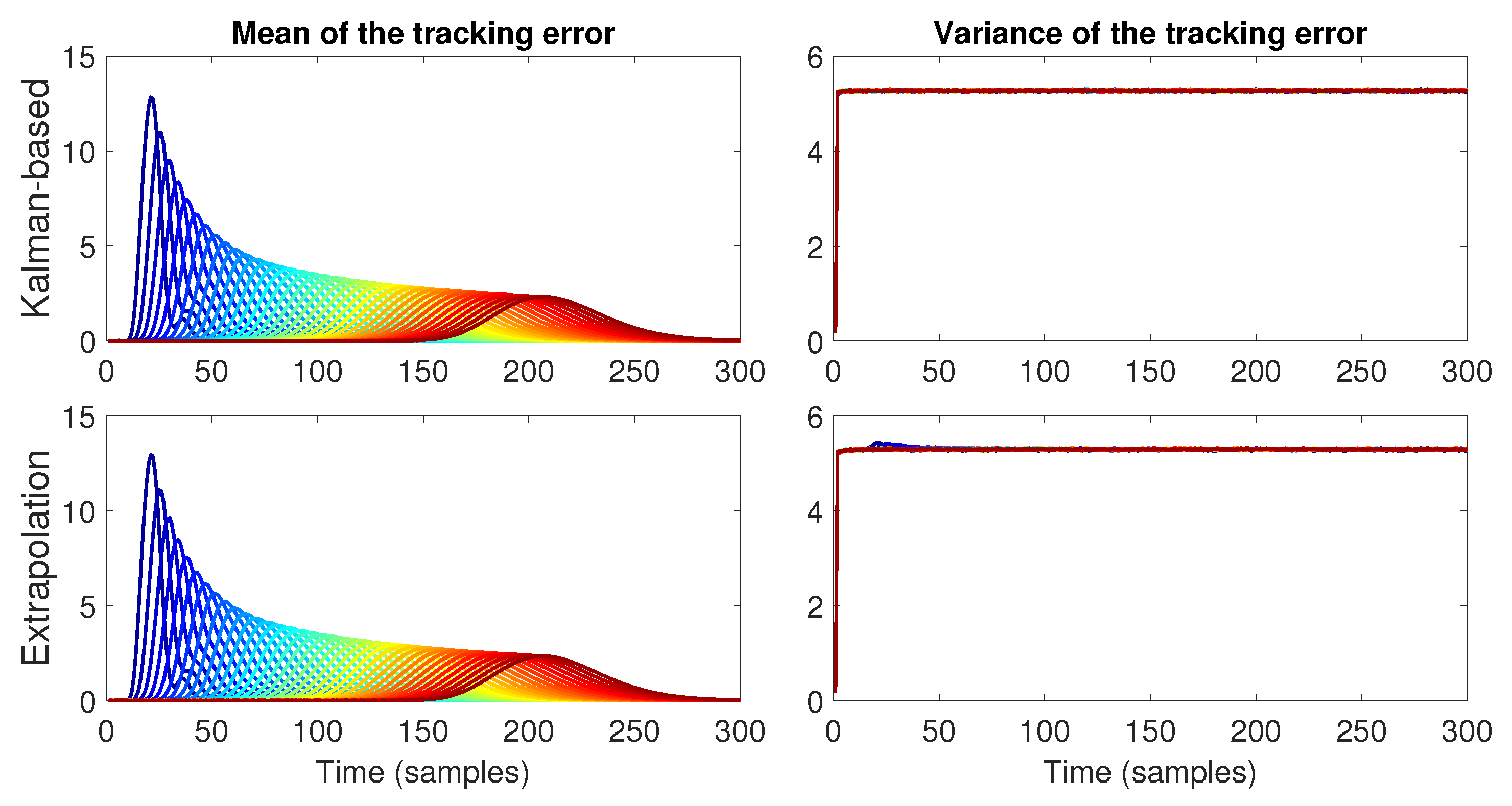
  • The performance of the proposed strategy is analyzed numerically for two cases for the data loss probability; a case with a constant data loss probability and another case where the transmission success is dependent on the inter-vehicle distance. As part of this analysis, we also compare the performance of our proposal with a simpler strategy based purely on linear extrapolation [9]. Our numerical results show that although both strategies can achieve string stability for the means and variances of both the tracking and estimation errors, the Kalman filtering-based approach produces better performance compared to the linear extrapolation strategy. Moreover, our proposed strategy is capable of achieving string stability for channels with higher data-loss probability values than those attainable using the extrapolation strategy.
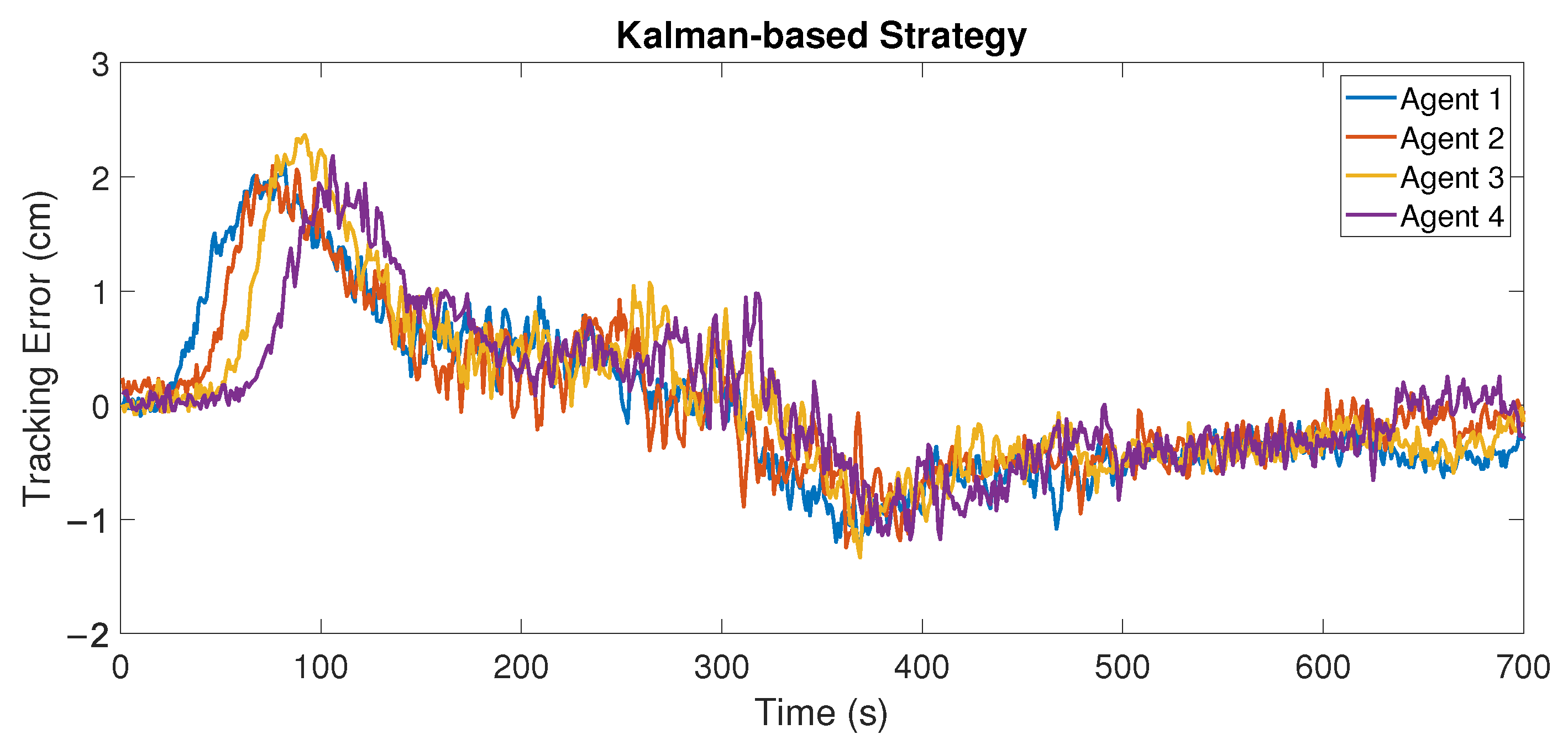
  • We also implement these strategies on the experimental platform PL-TOON [31,32], which is a low-cost platform with scale vehicles around 20 cm long that can is suitable for platooning studies. We show that both strategies can achieve tracking errors with string-stable performance, and although the comparison of these strategies does not demonstrate improvements, mainly due to sensor noise levels, the performance of the platoon is slightly better in terms of the variance when using the Kalman filter strategy.
This article is organized as follows. In Section 2, the problem setup is presented, which includes the platooning framework and the model for the communication channel that experiences random data loss. The proposed strategy and the one used for comparison purposes are described in Section 3. The performance of the two strategies is tested through simulations in Section 4, and the results of the experiments are presented in Section 5. Finally, the conclusions and future work are discussed in Section 6.

2. Platooning Problem Description

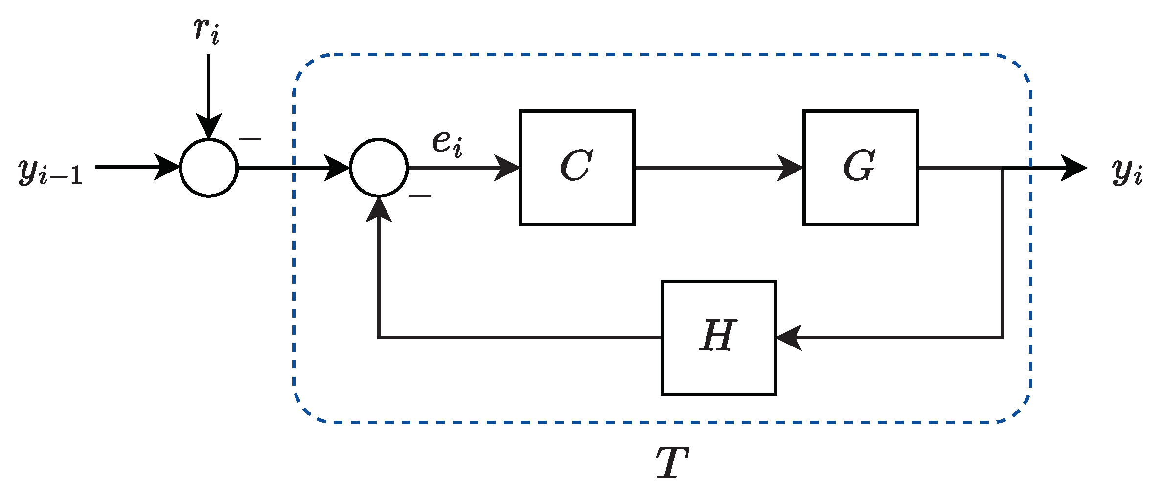
2.1. Platooning Setup with Ideal Communication

We consider a uni-dimensional platoon formed by M N vehicles using a predecessor-following topology. Each vehicle is identified using the index i = 0 , 1 , . . . , M 1 and follows the vehicle ahead while maintaining the desired inter-vehicle distance, except for the leader vehicle ( i = 0 ), which moves independently from the rest of the platoon. To perform this task, it is assumed that each vehicle can transmit some relevant information to the following vehicle through wireless communication. This is depicted in Figure 1, where i ( k ) represents the inter-vehicle distance between vehicle i and its predecessor.
In this work, we assume that the platoon depicted in Figure 1 is homogeneous, that is, each agent is described by the same dynamics. We consider that the dynamics of each agent are modeled by a discrete-time, linear time-invariant (LTI) system, described by the transfer function G ( z ) . Furthermore, each vehicle has the same local stabilizing controller described by the LTI system C ( z ) . We assume that G ( z ) and C ( z ) have a structure, where each one has integration and satisfies the condition that the product C ( z ) G ( z ) is strictly proper. These structures also guarantee that the product C ( z ) G ( z ) has double integration, which is a requirement for achieving adequate formation and perfect tracking of the leader vehicle velocity when the communication is ideal [33].
It is also assumed that at each time instant k Z , each vehicle is capable of measuring its own position, y i ( k ) , and obtaining its predecessor position, y i 1 ( k ) , and some additional data if needed, which are transmitted wirelessly. For this platooning setup, the local control loop should follow the predecessor vehicle and maintain the inter-vehicle distance as close as possible to a reference signal r i ( k ) . The inter-vehicle distance between vehicle i and its predecessor is given by
i ( k ) = y i 1 ( k ) y i ( k ) .
To reduce the collision probability between the vehicles when an unexpected event occurs, the distance with respect to the predecessor agent increases proportionally to its own velocity. The reference r i ( k ) has the following form
r i ( k ) = κ i + h [ y i ( k ) y i ( k 1 ) ] κ i + h v i ( k ) ,
where κ i is a constant that defines the minimum desired separation and the difference in its position with the previous sample y i ( k ) y i ( k 1 ) represents the rate of change of its position, which, in discrete time, is equivalent to the vehicle’s velocity v i ( k ) . This strategy is known as the constant time-headway spacing policy, where h > 0 is the time-headway constant [34].
We can assume, without altering the analysis, that κ i = 0 , which implies that the tracking error ζ i ( k ) corresponds to
ζ i ( k ) = y i 1 ( k ) y i ( k ) h y i ( k ) + h y i ( k 1 ) ,
and the error signal e i ( k ) that enters controller C ( z ) is given by e i ( k ) = ζ i ( k ) . These signals are not always identical, as explained later. In the Z-domain, e i ( k ) becomes
E i ( z ) = Y i 1 ( z ) Y i ( z ) [ ( 1 + h ) h z 1 ] .
We can state the equivalent local control loop shown in Figure 2, where H ( z ) = ( 1 + h ) h z 1 corresponds to a first-order FIR filter (finite impulse response) whose function is to enable the constant time-headway spacing policy and ensure that the string stabilization of the platoon is feasible [34]. In Figure 2, the closed-loop system T ( z ) is the transfer function between Y i 1 ( z ) and Y i ( z ) , which is given by
T ( z ) = G ( z ) C ( z ) 1 + G ( z ) H ( z ) C ( z ) .
Since the platoon is homogeneous, the system T ( z ) is identical for each agent and can be modeled as a discrete-time LTI system in state-space form as
x i ( k + 1 ) = A x i ( k ) + B y i 1 ( k ) + w i ( k ) ,
y i ( k ) = C x i ( k ) + q i ( k ) ,
where for the i-th agent, x i ( k ) is the closed-loop system state; y i 1 ( k ) is the predecessor vehicle position, which enters the i-th system (see Figure 3); and  y i ( k ) is the vehicle position. A, B, and C are the space-state matrices of the system, whereas w i ( k ) N ( μ w , P w ) and q i ( k ) N ( μ q , P q ) are the process and observation noise, respectively, which are second-order wide-sense stationary (WSS) stochastic processes that are mutually uncorrelated ( v N ( μ v , P v ) indicates that v is a random variable with a normal distribution, mean μ v , and covariance matrix P v ).

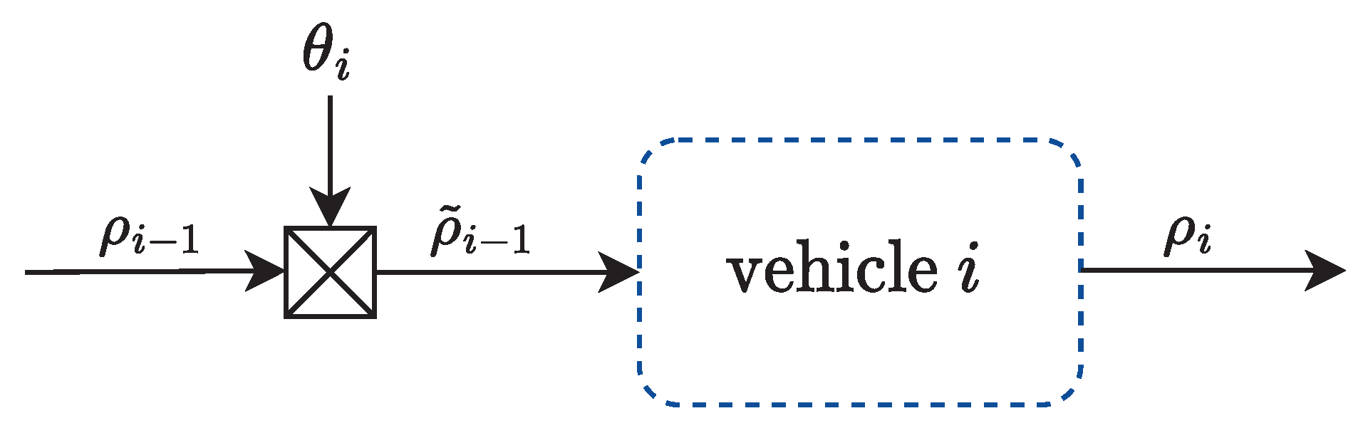
2.2. Platooning with Lossy Communication

2.2.1. Channel Model for Lossy Communications

We consider that each agent shares a data vector ρ i with the vehicle that follows it. We assume that the data transmitted ρ i ( k ) contain at least the vehicle position y i ( k ) but additional data can be included. This signal is transmitted wirelessly through an imperfect communication channel subject to random data loss. A common approach to modeling these lossy channels is to consider them to be defined by a Bernoulli process θ i { 1 , 0 } , where θ i ( k ) = 1 indicates that the data of the predecessor vehicle with index i 1 , denoted by ρ i 1 ( k ) , are received successfully at the vehicle with index i. On the other hand, when θ i ( k ) = 0 , the data are considered lost. The platoon including the channel model is shown in the scheme of Figure 3, where the input at the i-th vehicle is now the channel output. The i-th vehicle’s channel model is then given by
ρ ˜ i 1 ( k ) = θ i ( k ) ρ i 1 ( k ) ,
where ρ i 1 ( k ) is the channel input and ρ ˜ i 1 ( k ) is the channel output. It is noteworthy that vehicle i is aware of whether the data sent by the predecessor were received or not at a given instant. This is equivalent to assuming that vehicle i knows the state of θ i ( k ) .
The model described above is commonly used in the context of networked control systems [15,21]. It should be noted that in practical applications, the loss of transmitted data is not equivalent to receiving a zero measurement value. The Bernoulli variable θ i ( k ) in the channel model is an indicator for data loss and the value received by the receiver depends on the adopted protocol, which is determined by θ i ( k ) .
We consider two cases to define Pr { θ i ( k ) = 1 } , i.e., the probability of successful transmission of the communication channels.

Constant Probability

In this case, we assume that the probability of successful transmission in each vehicle is a constant p. Thus, we have p = Pr { θ i ( k ) = 1 } , which, in turn, implies that Pr { θ i ( k ) = 0 } = 1 p . This is the typical and simpler approach to modeling data loss in platooning [9,13,14] and represents the case where the transmission quality is not dependent on external factors such as the environment or the inter-vehicle distance.

Distance-Dependence Probability

A more realistic approach is to consider that the degradation in a wireless link has a direct relation to the separation distance [35]. In the case of a vehicle platoon with wireless communication, the quality of the transmitted signal is affected by the distance with respect to the preceding vehicle for a predecessor-following topology. Thus, it would be reasonable to consider that the transmission probability varies depending on the inter-vehicle distance, and thus Pr { θ i ( k ) = 1 } = p ( i ( k ) ) , where p ( i ( k ) ) is a function that characterizes the distance dependence. We consider that p ( i ( k ) ) is given by
p ( i ( k ) ) = α i ( k ) + β , i ( k ) 0 0 , i ( k ) > 0
for some parameters α and β , and with 0 being the maximum inter-vehicle distance that allows for a transmission probability higher than zero. In other words, p ( 0 ) = 0 .

2.2.2. Problems with Lossy Communication

Lossy communication should generate problems with the platooning task, mainly due to the fact that the measurement for the inter-vehicle distance is randomly lost. The tracking task is more difficult since the local controller in each vehicle only has access to y ˜ i 1 ( k ) = θ i ( k ) y i 1 ( k ) instead of y i 1 ( k ) , which implies that the controller input e i ( k ) is now given by
e i ( k ) = y ˜ i 1 ( k ) y i ( k ) h y i ( k ) + h y i ( k 1 ) ,
and thus e i ( k ) is not equal to the tracking error ζ i ( k ) in this scenario (see (3)). In the ideal communication case, both e i ( k ) and ζ i ( k ) are identical. However, when the communication is subject to random losses, this is no longer the case. The use of compensation strategies to deal with data loss is necessary for this scenario, and depending on the type of strategy used, different platoon performances can be achieved [9].
Moreover, not only the tracking task can be affected by data loss. Another important property in platooning problems known as string stability can be lost due to the effect of lossy communication. This property is detailed in the next section. In this article, we propose a new strategy based on the intermittent Kalman filter [19] and qualitatively evaluate its performance, with a special interest in observing whether or not it is capable of achieving string-stable behavior.

2.3. Platoon String Stability

String stability is normally observed in the behavior of the platoon’s tracking error. The expected behavior of a string-stable platoon is that the tracking error does not amplify as disturbances propagate along the string when the platoon size increases. An example of this for a simulated case with ideal communication and a properly designed local closed loop can be seen on the left side of Figure 4, where the position of each vehicle in the platoon is represented by colors, with blue representing the first agent and red representing the last agent.
Under ideal communication conditions for the described platooning setup, the string stability property admits an analytical definition. Indeed, it is not difficult to show that the error in (4) satisfies E i ( z ) = T ( z ) E i 1 ( z ) , which, in turn, implies that E n ( z ) = T ( z ) n 1 E 1 ( z ) . Considering that the closed-loop transfer function T ( z ) is a stable transfer function (the local controller C ( z ) is capable of stabilizing the closed loop), it is clear that the errors are not increasing in amplitude if | T ( e j ω ) | 1 , ω [ 0 , 2 π ] . This is equivalent to requiring T ( z ) 1 . We consider the following definition (similar to [10]):
Definition 1. 
The sequence of the transfer functions M n , n N is said to be string stable if there exists c R independent of n such that M n c for all n. Otherwise, we say that it is string unstable.
Clearly, for the given setup, the platoon is string stable in the deterministic case whenever T ( z ) 1 , as the associated sequence of the transfer functions is T n 1 ( z ) . On the other hand, if  T ( z ) > 1 , the platoon is string unstable as the interconnected system causes the tracking errors to increase in amplitude along the platoon. This is not desirable in practice since whenever the platoon size reaches a certain threshold, the magnitude of the tracking errors that increase out of proportion may cause the vehicles to collide with one another. For the previously described system with double integration in the product C ( z ) G ( z ) , it is not possible to achieve T ( z ) 1 if h = 0 . This is the reason that H ( z ) from the time-headway strategy is included in the closed loop. It is possible to guarantee the platoon’s string stability, as the chosen value of h is greater than the critical value [10,34].
Remark 1. 
In this and subsequent sections, the time behaviors of the platoon are displayed in graphs using a color-coded system. The initial follower is indicated in dark blue and the final follower is indicated in dark red. The vehicles in between are shown in the order specified in the color bar at the bottom of Figure 4. The colors, proceeding from left to right, correspond to the increasing indices of the vehicles along the line. The color bar is omitted in the remaining figures.
Under conditions where the communication is no longer perfect, the platoon string stability analysis stops being deterministic due to the randomness of the losses θ i ( k ) , and the deterministic condition T ( z ) 1 is no longer sufficient. Indeed, the successful transmission probability has a considerable effect on the sequence of the tracking errors, as observed in the right plot in Figure 4, where the probability is set to p = 0.8 and the resulting signals are more distorted compared to the ideal case, with peaks of a random nature. This is why the usual definitions for string stability cannot be used. Unfortunately, a standard analytical definition for string stability in a stochastic setting is missing in the current literature. Instead, in these scenarios, it is common to qualitatively analyze the mean and variance of the tracking error in order to observe the string-stable behavior [9,10,14]. In particular, in this paper, we qualitatively study string stability by analyzing the mean μ ζ i ( k ) and variance σ ζ i ( k ) 2 of the tracking error.
It is also important to mention that the use of a compensation strategy or policy to replace lost data is inevitable and may affect the string stability of the platoon [9]. For example, a simple strategy to use when ρ i ( k ) = y i ( k ) is to consider the communication channel output y ˜ i 1 ( k ) directly as an input to the system T ( z ) . This case results in behavior such as that shown in Figure 5, where even if the transmission probability is high ( p = 0.99 ), the magnitude of the tracking error increases significantly. Thus, this compensation scheme is not compatible with the notion of string stability. It is, therefore, relevant to propose compensation strategies that have better performance than the one shown in the example in Figure 5.

2.4. PL-TOON Implementation Considerations

The experimental implementation was carried out on the PL-TOON platform [31]. Each agent on the PL-TOON platform has a frontal time-of-flight sensor VL53L0X to measure the distance with respect to the predecessor vehicle and a second optical sensor ANDS3080 to measure the agent’s velocity independently. The distance sensor has a resolution of 1 mm (which varies depending on the ambient conditions) and a sampling period of 20 ms. The second sensor is an optical sensor, similar to that used in an optical mouse, which is used to measure the displacement of the agent, and then by measuring the elapsed time, it estimates the instantaneous velocity of the agent. Each of these sensors also has intrinsic measurement noise that has to be taken into account at the moment of performing the experiments. The main micro-controller unit of each vehicle is an ESP32, which has wireless capabilities that are used to broadcast data to the rest of the agents. A photo of part of the experimental setup is shown in Figure 6, where the individual components previously described are labeled. The details of these units and their sub-routines were explained in our previous work [31].
The model G ( z ) considered for this experiment is based on the model of the agents on the PL-TOON platform, which have the following structure (see [32]):
G ( z ) = b z ( z 1 ) ( z a ) ,
where a and b are constant parameters. We also use a PI controller since it is usually sufficient for obtaining acceptable results, which have the form:
C ( z ) = ( K p + K i ) z K p z 1 ,
where K p , K i , and K p are the design parameters. The values of a and b are obtained after performing a parameter identification procedure in one of the platform’s vehicles, which consists of exciting the agents in an open-loop setup with a step input, and then using the distance sensor data to calculate the gain and settling time of the response, allowing calculating a and b (see, for instance, [32]). This standard identification procedure yields b = 0.0020131 and a = 0.713 for the vehicle dynamics G ( z ) .
On the other hand, we also performed experiments to determine the data loss communication features on the platform and determine the probability of successful transmission p ( i ( k ) ) depending on the inter-vehicle distance. To obtain this function, we performed successive experiments by transmitting 1000 packets from one PL-TOON agent to obtain the total number of received packets in another agent for different inter-vehicle distances. After a number of iterations, we obtained the data shown in Figure 7 and performed a linear regression to obtain a transmission probability curve for our operating point, which is as follows:
p ( i ( k ) ) = 0.0025 i ( k ) + 0.9786 , i ( k ) 0 0 , i ( k ) > 0
The difference between the PL-TOON capabilities and those assumed in the problem setup is that the sensor measures the relative distance i ( k ) using the predecessor vehicle and not the absolute position y i ( k ) . In practice, the results from both the model and the experimental agent would be similar; however, the algorithm for some of the compensation strategies would need to be adapted to consider the difference in the measured variables. This is discussed in Section 3.3.

3. Compensation Strategies

In this work, we use a strategy where the missing data ρ i 1 ( k ) is replaced with an estimate ρ ^ i 1 ( k ) . The output of the compensation stage, which is referred to as ρ ¯ i 1 , is used in the control loop of the i-th vehicle and is given by
ρ ¯ i 1 ( k ) = θ i ( k ) ρ ˜ i 1 ( k ) + [ 1 θ i ( k ) ] ρ ^ i 1 ( k ) .
Thus, the channel output of the system is identical to the transmitted signal from the predecessor vehicle when the communication is successful, that is, ρ ¯ i 1 ( k ) = ρ i 1 ( k ) for θ i ( k ) = 1 (in this case, ρ ˜ i 1 ( k ) = ρ i 1 ( k ) ), and in cases where the transmission fails and the data are lost ( θ i ( k ) = 0 ), the output corresponds to an estimate ρ ^ i 1 ( k ) of some kind, with  ρ ¯ i 1 ( k ) = ρ ^ i 1 ( k ) .
To calculate the estimate ρ ^ i 1 ( k ) , two types of estimations are considered. The first is the simpler of the two and is based on linear extrapolation. Its performance was studied in [9] and it is used here for comparison purposes. The second type of estimation is the main contribution of this paper and corresponds to a strategy based on the intermittent Kalman filter, allowing us to consider the data-loss phenomenon as part of the estimation problem [19,20].

3.1. Linear Extrapolation

In this case, it is assumed that ρ i ( k ) = y i ( k ) . Since one of the objectives of the vehicle platoon is to achieve a constant velocity, the vehicles are expected to converge to a ramp-shaped trajectory y i ( k ) . Thus, using linear extrapolation for the estimate y ^ i 1 ( k ) of the position is appropriate in this context [9]. This strategy can be implemented in the following way:
y ^ i 1 ( k ) = y ˜ i 1 ( k ) if θ i ( k ) = 1 , y ¯ i 1 ( k 1 ) + Δ ( k ) if θ i ( k ) = 0 .
where Δ ( k ) is the estimate of the traveled distance between the instants k 1 and k, and can be calculated as Δ ( k ) = y ¯ i 1 ( k 1 ) y ¯ i 1 ( k 2 ) . Hence, using this strategy, the input to the system T can be written as
y ¯ i 1 ( k ) = θ i ( k ) y ˜ i 1 ( k ) + [ 1 θ i ( k ) ] 2 y ¯ i 1 ( k 1 ) y ¯ i 1 ( k 2 ) .
Furthermore, the term multiplied by ( 1 θ i ( k ) ) is equivalent to the output of a second-order FIR filter ( 2 z 1 ) / z 2 with y ¯ i 1 ( k ) as input. This strategy can be implemented as shown in the block diagrams in Figure 8 and Figure 9, where F e x t corresponds to this compensation strategy.

3.2. Strategy Based on the Intermittent Kalman Filter

The second strategy for data loss compensation is the main contribution of this paper and considers that the i-th vehicle computes an estimate of the preceding vehicle’s data to replace it in case of loss based on a local model of the ( i 1 ) -th vehicle. The input to the system T, denoted by y ¯ i 1 ( k ) , is given by
y ¯ i 1 ( k ) = θ i ( k ) y ˜ i 1 ( k ) + [ 1 θ i ( k ) ] y ^ i 1 ( k ) ,
where y ^ i 1 ( k ) denotes the estimates of the preceding vehicle’s position. Since the platoon is homogeneous, to obtain y ^ i 1 ( k ) , we use the following model for the vehicle i 1
x i 1 ( k + 1 ) = A x i 1 ( k ) + B y ¯ i 2 ( k ) + w i 1 ( k ) ,
y i 1 ( k ) = C x i 1 ( k ) + q i 1 ( k ) ,
which is essentially (6), but in (17), the input to the vehicle i 1 corresponds to the signal y ¯ i 2 , that is, the output from the compensation scheme of the preceding vehicle. Thus, for the implementation of this strategy in vehicle i, we assume that the vehicle ahead also transmits the information y ¯ i 2 , along with its position y i 1 , and hence, the channel input is ρ ( k ) = [ y i 1 ( k ) y ¯ i 2 ( k ) ] . To estimate y i 1 , we first estimate the state in (17) based on the Kalman filter with intermittent observations [19] but adapted for the context of this problem. Furthermore, when the transmission fails ( θ i ( k ) = 0 ), not only is y i 1 ( k ) lost but  y ¯ i 2 ( k ) is also lost. In this case, the input y ¯ i 2 ( k ) also has to be replaced with an appropriate estimate. Indeed, the inputs for this compensation stage are y ˜ i 1 ( k ) = θ i ( k ) y i 1 ( k ) and y ¯ ˜ i 2 ( k ) = θ i ( k ) y ¯ i 2 ( k ) . However, using a Kalman filter with intermittent observations to estimate y ¯ i 2 ( k ) would imply the computation of a spatially iterative filter that depends on the outputs of all the preceding vehicles. However, this cannot be implemented under the communication topology considered in this paper, where we only have access to the information sent from the predecessor vehicle. Thus, for the estimate of y ¯ i 2 ( k ) , the previously described linear extrapolation is applied to this signal, that is, the estimator based on the Kalman filter with intermittent observations uses the estimate y ¯ ^ i 2 ( k ) as its input, where
y ¯ ^ i 2 ( k )   = θ i ( k ) y ¯ ˜ i 2 ( k ) + [ 1 θ i ( k ) ] ( 2 y ¯ ^ i 2 ( k 1 ) y ¯ ^ i 2 ( k 2 ) ) ,
with y ¯ ˜ i 2 ( k ) = θ i ( k ) y ¯ i 2 ( k ) . Then, considering that x ^ i 1 ( k | j ) corresponds to the estimate of the state x i 1 ( k ) and using the information available up to the instant j, the prediction step is implemented using
x ^ i 1 ( k + 1 | k ) = A x ^ i 1 ( k | k ) + B y ¯ ^ i 2 ( k ) + μ w ,
y ^ i 1 ( k ) = C x ^ i 1 ( k | k 1 ) + μ q ,
whereas the filter update step is given by
x ^ i 1 ( k | k ) = x ^ i 1 ( k | k 1 ) + θ i ( k ) K i 1 ( k ) [ y ˜ i 1 ( k ) y ^ i 1 ( k ) ] ,
K i 1 ( k ) = P i 1 ( k | k 1 ) C ( C P i 1 ( k | k 1 ) C + P q ) 1 ,
P i 1 ( k + 1 | k ) = A ( I θ i ( k ) K i 1 ( k ) C ) P i 1 ( k | k 1 ) A + P w ,
where K i 1 ( k ) is the filter gain and  P i 1 ( k | j ) is related to the conditional covariance matrix of the state estimation error. Clearly, the terms in (20)–(22) depend on θ i ( k ) and, generally, are not expected to converge. The fact that P i 1 ( k + 1 | k ) is a random variable is one of the important differences between the Kalman filter with intermittent observations and the standard Kalman filter and is caused by random data dropouts [19].
Block diagrams of the proposed strategy are shown in Figure 10 and Figure 11, where the block K F represents the previously described Kalman filter and F K F refers to the whole compensation strategy, including the linear extrapolation for the input.

3.3. Strategies for Relative Distance Model

Both strategies described in the previous sections assume that the absolute positions y i ( k ) are available. Thus, to implement this strategy on the PL-TOON experimental platform, the algorithm has to be adapted, as we only have access to the relative distance i ( k ) = y i 1 ( k ) y i ( k ) .

3.3.1. Linear Extrapolation

Note that for the distance model of a PL-TOON agent, for ramp-shaped trajectories, the relative distance will be constant in the steady state. However, since i ( k ) = y i 1 ( k ) y i ( k ) but the measurement is ˜ i ( k ) = θ i ( k ) i ( k ) , the equivalent implementation of the linear extrapolation in (14) in this model is
^ i ( k ) = ˜ i ( k ) if θ i ( k ) = 1 , ¯ i ( k 1 ) if θ i ( k ) = 0 .
where ^ i ( k ) is the estimation obtained from this method and ¯ i ( k ) = θ i ( k ) ˜ i ( k ) + ( 1 θ i ( k ) ) ^ i ( k ) . This strategy is simply holding the previous value in case of data loss, which is a simple but common strategy for estimating a signal that is expected to be or is expected to converge to a constant value [15]. An implementation of this strategy written in pseudo-code is shown in Algorithm 1.
Algorithm 1 Data replacement using linear extrapolation (holding previous distance)
  • ˜ i ( k ) sensor measurement
  • θ i ( k ) detect if the data were lost
  •  
  • if  θ i ( k ) = 0  then replace data with a linear extrapolation estimate
  •      ^ i ( k ) PreviousDistance( ¯ i ( k ) )
  •      ¯ i ( k ) i ^ ( k )
  • else
  •      ¯ i ( k ) ˜ i ( k )                                                                         ▹ data received successfully
  • end if
  • e i ( k ) ¯ i ( k ) h v i ( k )                                                   ▹ calculate error for control loop
  •  
  • procedure PreviousDistance( ¯ i ( k ) )
  •      ^ i ( k ) ¯ i ( k 1 )                                                                   ▹ measurement estimation
  •     return  ^ i ( k )
  • end procedure

3.3.2. Strategy Based on the Intermittent Kalman Filter

Using the state-space representation of the system in (6) as a basis, we define an alternative state x i * ( k ) = x i 1 ( k ) x i ( k ) . This way, and considering the homogeneity of the platoon, we can obtain the inter-vehicle distance as
i ( k ) = C ( x i 1 ( k ) x i ( k ) ) + q i 1 ( k ) q i ( k ) = C x i * ( k ) + q i * ( k ) ,
where q i * = q i 1 q i is the new observation noise. Similarly, we can obtain the prediction step in the following way
x i * ( k + 1 ) = A x i * ( k ) + B i 1 ( k ) + w i * ( k ) ,
where w i * = w i 1 w i is the new process noise. Since both q i * and w i * are linear combinations of noise from different vehicles, their statistics are now q i * N ( μ q i 1 μ q i , P q i 1 + P q i ) and w i * N ( μ w i 1 μ w i , P w i 1 + P w i ) .
Here, we interpret that the distance i is the output of an LTI system with input i 1 . This is virtually equivalent to the already described platoon setup with 0 = u 0 y 0 , where u 0 is the actuation signal on the lead vehicle and  y 0 is its resulting position due to the same actuation. Hence, the goal is to use this system to estimate the state of this system and then the relative distance i when there is random data loss. Since in practice, we have access to i at all times through the vehicle’s sensor, the random data loss could be interpreted as a sensor malfunction. However, similar to the original setup, for this model, we also require the input i 1 , which is the relative distance measured by the preceding vehicle, and this variable has to be transmitted wirelessly; thus, it is subject to random data loss due to the communication channel.
Adapting (19) to these new equations results in the following estimate
x * ^ i ( k + 1 | k ) = A x * ^ i ( k | k ) + B ¯ ^ i 1 ( k ) + μ w * ,
^ i ( k ) = C x * ^ i ( k | k 1 ) + μ q * .
Then, the filter update step is given by
x * ^ i ( k | k ) = x * ^ i ( k | k 1 ) + θ i ( k ) K i ( k ) [ ˜ i ( k ) ^ i ( k ) ] ,
where ˜ i ( k ) = θ i ( k ) i ( k ) , and  ¯ ^ i 1 ( k ) is the estimate resulting from the linear extrapolation. The output of the filtering process is then ¯ i ( k ) = θ i ( k ) ˜ i ( k ) + ( 1 θ i ( k ) ) ^ i ( k ) . The equations for the gain K i ( k ) and the matrix P i ( k | k 1 ) remain the same as in (21) and (22), respectively, but using the covariances P q * and P w * instead of P q and P w . The equivalent implementation in pseudo-code is shown in Algorithm 2. Note that compared to Algorithm 1, here, the procedure to calculate the estimation using the Kalman filter with intermittent observations is called at each cycle to keep updating the state x ^ i * ( k ) and the matrix P i ( k ) .
Algorithm 2 Data replacement using strategy based on intermittent Kalman filter
  • ˜ i ( k ) local sensor measurement
  • ¯ ˜ i 1 ( k ) predecessor vehicle measurement                  ▹ obtained via wireless broadcast
  • θ i ( k ) detect if the data were lost
  •  
  • ^ i ( k ) IntKalmanFilter( ˜ i ( k ) , ¯ ˜ i 1 ( k ) , x ^ i * ( k ) , P i ( k ) , θ i ( k ) )
  • if  θ i ( k ) = 0  then replace data with Kalman filter estimate
  •      ¯ i ( k ) i ^ ( k )
  • else
  •      ¯ i ( k ) ˜ i ( k )                                                                            ▹ data received successfully
  • end if
  • e i ( k ) ¯ i ( k ) h v i ( k )                                                      ▹ calculate error for control loop
  •  
  • procedure IntKalmanFilter( ˜ i ( k ) , ˜ i 1 ( k ) , x ^ i * ( k ) , P i ( k ) , θ i ( k ) )
  •      K i ( k ) P i ( k ) C ( C P i ( k ) C + P q ) 1                                                ▹ Kalman gain
  •      ^ i ( k ) C x ^ i * ( k ) + μ q                                                                ▹ measurement estimation
  •     if  θ i ( k ) 0  then proceed with the update step
  •          x ^ i * ( k ) x ^ i * ( k ) + K i ( k ) ( i ( k ) ^ i ( k ) )
  •          P i ( k ) P i ( k ) K i ( k ) C P i ( k )
  •          ¯ ^ i 1 ( k ) ¯ ˜ i 1 ( k )
  •     else                                                                                                                            ▹ data is lost
  •          ¯ ^ i 1 ( k ) PreviousDistance( ¯ ˜ i 1 ( k ) )
  •     end if
  •      x ^ i * ( k ) A x ^ i * ( k ) + B ¯ ^ i 1 ( k ) + μ w                                                        ▹ prediction step
  •      P i ( k ) A P i ( k ) A + P w
  •     return  ^ i ( k )
  • end procedure

4. Simulation Results

In this section, we report the numerical results of the performance of both compensation strategies for a vehicle platoon subject to random data loss that we previously described.
Since the setup is of a stochastic nature due to the presence of random data loss in the transmission, the moments of the tracking error ζ i ( k ) are analyzed. To evaluate the performance of the tracking, first, it is required that the controller C ( z ) achieves mean square stability (MSS), that is, that both the mean and variance of the error converge [14]. A second condition is that the mean of the tracking error for each vehicle must follow
lim k μ ζ i ( k ) = E ζ i ( k ) = 0 , i = { 1 , . . . , M 1 } ,
with M being the total number of vehicles in the platoon and the operator E · indicating the expected value. To compare both compensation strategies quantitatively, we use the variance of the tracking error
σ ζ i 2 ( k ) = E ( ζ i ( k ) E ζ i ( k ) ) 2 .
Since the mean converges to zero, the strategy that presents less variance is considered to have achieved better performance, as it translates into a more fluid behavior of the platoon, and thus it reduces the collision probability between agents due to the random losses. Lastly, a behavior of the error signal that is compatible with string stability is considered to compare the strategies.
In the same way, to evaluate the quality of the estimation, we analyze the estimation errors from both strategies. An error is defined as
ε i ( k ) = y i ( k ) y ¯ i ( k ) , i = { 1 , . . . , M 1 } ,
where y ¯ i is the estimate resulting from the compensation stage in the ( i + 1 ) -th vehicle, whereas y i is the output of the i-th vehicle before going through the communication channel. The comparison is similar to ζ i ( k ) , that is, the strategy that achieves μ ε ( k ) = 0 and a smaller variance σ ε ( k ) 2 will achieve a better estimate.
For the simulation, we consider the linear model obtained for the PL-TOON agents, that is, each vehicle has a transfer function representation G ( z ) and controller C ( z ) given by
G ( z ) = 0.0020131 z ( z 1 ) ( z 0.713 ) , C ( z ) = 40 z 20 z 1 .
Furthermore, the block H ( z ) has a time-headway constant value of h = 5 , which guarantees string stability in the case with no communication loss for these dynamics [10]. On the other hand, the noises w and q have a zero mean and a small variance.
Due to the vehicle-leader trajectory being deterministic, for the simulation, it starts from rest and then accelerates forward for a short period of time in such a way that the velocity gradually changes, as shown in Figure 12.
The performance of the vehicle platoon for a platoon size of M = 40 is evaluated numerically through a Monte Carlo simulation with N = 5 × 10 5 realizations and for different values of the successful transmission probability p.

4.1. Constant Transmission Probability

In this first case, with a transmission probability of p = 0.95 , it can be observed in Figure 13 that the mean of the tracking error has string-stable behavior using both the Kalman filter strategy and the extrapolation strategy. In other words, the peak value of μ ζ i ( k ) decreases with the vehicle position within the platoon, i.e., with i. The same behavior can be observed for the variance of the tracking error σ ζ i ( k ) ; however, using the Kalman strategy results in a much smaller magnitude in comparison to the extrapolation strategy (close to 1000 times). This indicates that the intermittent Kalman filter strategy delivers better performance for this example. The same behavior is present in the estimation error ε i ( k ) (see Figure 14), which has string-stable behavior for both its mean and variance. However, now both the mean and variance have a smaller magnitude in the case of the Kalman strategy due to the Kalman filter reducing the estimation error.
On the other hand, when the transmission probability decreases to a value of p = 0.75 , it can be seen in Figure 15 that the mean of the tracking error μ ζ i ( k ) is still compatible with the notion of stochastic string stability for both strategies. The difference now is that the amplitude values of the variance increase significantly in comparison to the previous case. However, the variance of the Kalman filter is of a smaller magnitude in comparison to the extrapolation strategy; thus, this behavior is conserved from the previous case. It is also noteworthy that the difference in magnitude of the variances of both strategies decreases and now, the Kalman strategy is only about 100 times smaller than the extrapolation strategy. A similar situation is present in the estimation error shown in Figure 16, where it is shown that the mean and variance of the Kalman strategy result in a smaller estimation error and that the difference in magnitude between both strategies is not as large as the previous case for p = 0.95 . In addition, the overall peak values of both the mean and variance increase with the decrease in the successful transmission probability.
Remark 2. 
The spikes in the variances of samples 200–250, as seen in Figure 15 and Figure 16, correspond to numerical issues from the Monte Carlo simulation rather than as a result of the use of the compensation schemes. Nonetheless, these spikes do not affect the qualitative assessment of these Figures, as the difference in the performance of these two strategies is quite clear, as we described previously. Such spikes also appear and are more significant in the figures below, where the platoons are string unstable or close to instability.
Now, we reduce the time-headway constant to h = 4 , which is a value that still ensures string stability for the deterministic case but is much closer to the instability threshold. We also increase the number of vehicles to M = 400 and simulate using the same transmission probability of p = 0.75 . In this scenario, we can see from the results shown in Figure 17 that for the Kalman-based strategy, the mean of the tracking error μ ζ i ( k ) behaves in a string-stable manner, even for a large number of vehicles. The same can be said of the variance of the tracking error σ ζ i ( k ) since its peak value decreases across the platoon. In contrast, when analyzing the extrapolation strategy, it can be observed that now the mean is string unstable since we can see a clear amplification of the tracking error after 500 samples, which, in turn, generates oscillations near the end of the platoon. This behavior can be corroborated further by observing the variance of this strategy, which clearly increases with the number of vehicles in the platoon.
On the other hand, Figure 18 shows the results of the mean and variance of the estimation error ε i ( k ) . It can be observed that similar behavior occurs when the Kalman-based strategy achieves a lower mean and variance than the extrapolation strategy, and additionally, the mean of the latter shows string-unstable behavior. This example illustrates a clear benefit of using the Kalman-based strategy over the extrapolation strategy for the data replacement since, when the data transmission probability is relatively low (as shown with p = 0.75 ), the linear extrapolation strategy scheme exhibits string-unstable behavior, whereas the Kalman-based strategy is still able to maintain behavior compatible with string stability for the same transmission probability p. Thus, this suggests that the proposed strategy has a higher tolerance for communication failure and can achieve good performance for the vehicle platoon in scenarios where the extrapolation strategy is not even able to achieve string stability.

4.2. Distance-Dependent Transmission Probability

Rather than having a constant transmission probability, we now perform simulations where the transmission success rate p is dependent on the inter-vehicle distance, as we described in Section 2.2.1. Hence, we utilize the function p i ( i ( k ) ) defined in (12). The initial reference for the lead vehicle is the same as in the previous simulation with constant p. The time evolution of the probability p i ( i ( k ) ) is shown in Figure 19, where 10,000 trials were performed and then averaged to obtain the mean. It can be observed that at rest, the vehicles start with a value of p i ( i ( k ) ) > 0.95 and after the leader vehicle starts to accelerate, the value of p i ( i ( k ) ) gradually starts decreasing until it reaches a value of p i ( i ( k ) ) = 0.85 when the platoon achieves constant velocity. It is important to note that in this case, the value of p i ( i ( k ) ) is highly dependent on the initial conditions for a platoon setup with a time-headway spacing policy due to the inter-vehicle distance being proportional to the vehicle velocities. Thus, if the velocity is higher, the spacing between the vehicles will increase and as a result, the transmission probability p i ( i ( k ) ) will also decrease.
The error evolution for this case is shown in Figure 20. We can see that the results are similar to the case with constant p, where the mean behaves in a string-stable manner in both strategies and the Kalman-filtering scheme presents a smaller variance in comparison to the extrapolation strategy. It can also be observed that compared to the constant probability case with p = 0.95 , the variance seems noisier and has higher amplitude values. In the case of the estimation error, we can see the same tendency as before as shown in Figure 21, where the Kalman-based strategy presented lower mean and variance values.

5. Experimental Results

In this section, we report the results obtained from testing both strategies on the PL-TOON platform. The setup consisted of one lead vehicle and four following vehicles. Each vehicle transmitted its distance sensor information to the following vehicle, which was then used by the proposed strategy. It is important to highlight that in the experimental setup, both sensors may have been affected by intrinsic noise given the nature of the sensors. The model and controller of each agent were described in Section 4. Naturally, our experimental results are based on the analysis of the time evolution of the tracking error for a few trials in different setups rather than statistical analyses, as in the Monte Carlo-based simulation results. To implement the replacement strategies in the vehicles, we used the schemes derived in Section 3.3 and considered the data losses on the distance signal rather than the position signals, as described previously. We also emulated the losses in the agents’ micro-controller units to have more control over the value of the failure probabilities. We only considered the case with constant probabilities, which were simpler to implement.

5.1. Experiment 1

For the first experiment, starting from rest and with each agent in the desired formation, we changed the leader’s distance reference to an obstacle. This caused it to accelerate for a few seconds, which, in turn, produced a disturbance that propagated along the platoon formation. Then, the same experiment was repeated in the opposite direction. For this scenario, we used a constant transmission probability of p = 0.85 and a constant time-headway value of h = 5 . The results using the Kalman strategy are shown in Figure 22. It can be seen that the tracking error was compatible with string stability due to the error decreasing its peak amplitude at each vehicle. On the other hand, Figure 23 shows the same results but for the extrapolation strategy, where the tracking error also performed in a string-stable manner.

5.2. Experiment 2

In this case, we performed an experiment using a moving platoon since the differences between the strategies would be more noticeable if the leader’s speed varied continuously over time. The transmission probability was also set to a relatively low value of p = 0.7 to increase the likelihood of using the estimated values for the duration of the experiments. For the leader vehicle, we set its velocity as shown in Figure 24. From rest, it started to accelerate gradually in an exponential shape and then slowly decreased its velocity in the same way. This exponential-shaped velocity was chosen to highlight the differences between the proposed Kalman strategy and the simpler linear extrapolation strategy.
The experimental results of the resulting tracking error for the platoon are shown in Figure 25 and Figure 26 for the Kalman and extrapolation strategies, respectively. Each plot shows the mean of the tracking error for the eight trials of the experiment, which is denoted by ζ ¯ i ( k ) , and we calculate the integral square error (ISE) index defined as 1 N k = 0 N 1 ζ ¯ i ( k ) 2 , with N being the total number of samples. The resulting values are shown in Table 1 for each of the vehicles after the leader, and for the comparison of both strategies. In this case, it can be observed that the better performance of the Kalman strategy over the extrapolation strategy was not as clear as in the simulations, and overall, the most noticeable improvement was that the former achieve a lower noise variance than the latter.

5.3. Discussion about Noise Level

The main discrepancy between the experimental results and the simulations was due to the presence of intrinsic noise in the sensing devices. The PL-TOON platform agents have two sources of measurement noise, namely the distance sensor and the local velocity sensor, which are described in Section 2.4. The simulations were conducted with low noise variance for both P w and P q to better highlight the impact of random data loss and the proposed strategies on the error variance. When the noise variance was too high, the variance resulted in the Monte Carlo simulation converging to the constant noise value, and the variance caused by the data loss was overshadowed, as shown in Figure 27. Additionally, to obtain the experimental results, we performed a few trials, unlike the numerical results, which allowed us to easily perform thousands of trials to properly calculate the error statistics. Hence, the presence of noise in the scaled-down experimental platform makes it challenging to observe a significant improvement from using the Kalman strategy. However, the difference between the strategies would be more pronounced if they were implemented in an experimental platform with heavier vehicles or on a more noise-resistant platform. The experimental platform also provided an opportunity to address implementation issues and evaluate the effectiveness of the proposed strategy in dealing with data loss in the communication channel.

5.4. Discussion about Other Potential Issues in Real Scenarios

Beyond the implementation on the PL-TOON platform, in real-world scenarios, there are several circumstances that may limit the application of our proposed algorithm. However, extending our framework to address some of these potential problems is also possible. Some of these issues are as follows:
  • In practice, heterogeneous platoons are expected to be more common than homogeneous ones. This implies that the models of the vehicles G i are generally different, which is beyond our framework setup. One way to deal with this is to design stabilizing controllers C i such that the closed-loop system T is common to all vehicles in the platoon, if possible. Another approach is to extend our setup to heterogeneous platoons by considering a different model of the preceding vehicle in our derivations.
  • Our approach requires estimating the previous vehicle information, which implies having an accurate model of such a vehicle. Model uncertainty may yield a poor estimation. To deal with this issue, collaborative systems identification algorithms can be included in order to reduce model uncertainty [36], as well as the inclusion of robust estimation techniques [37].
  • In our setup, we assume linear models. In practice, general models are expected to be nonlinear; hence, our setup cannot be straightforwardly applied. One solution is to use feedback-linearization techniques [38] or obtain a closed-loop linear model. Another alternative is to extend our approach by considering an estimator for nonlinear systems such as the unscented Kalman filter (UKF) with intermittent observations [39].
  • The inter-vehicle communication channels can suffer from different types of phenomena that can affect the performance of the platoon beyond data loss. These phenomena include random delays, fading, signal-to-noise ratio limitations, and cyber attacks, among others. Our approach could be extended to include tools from networked control systems theory to reduce the effect of such communication issues on the control performance (see, e.g., [40,41,42,43,44]).

6. Conclusions and Future Work

In this work, we proposed a new compensation strategy for a homogeneous vehicle platoon with inter-vehicular communication subject to random data loss. The algorithm was based on the intermittent Kalman filter enriched with a linear extrapolation stage. Through simulations and experiments, we studied its performance and compared it to the performance of an existing strategy based purely on a linear extrapolation scheme. From the simulation results, it was observed that the platoon stayed string stable in the mean and variance of the tracking error for both the strategy based on the intermittent Kalman filter and the one based on a linear extrapolation strategy, with high values of the successful transmission probability ( p > 0.9 ) and a conservative value of the time-headway constant of h = 5 used as the platoon parameters. However, there was a clear improvement of ≈ 10 3 and ≈ 10 2 times less variance for the Kalman filtering-based strategy compared to the extrapolation-based strategy when p = 0.9 and p = 0.75 , respectively. It seems likely that there exists an infimal value of the transmission probability that achieves a well-behaved platoon for any given value of h in this configuration [10]. Moreover, when h = 4 , which is close to the infimal value for deterministic string stability, the Kalman strategy can achieve string stability, even for values of p = 0.75 , maintaining moderate variance values of the tracking and estimation error, whereas the extrapolation-based strategy cannot even achieve string stability. A similar situation was observed for the case when the transmission probability depended on the inter-vehicle distance, where the Kalman-based strategy showed better performance in terms of the variance but resulted in a noisier error in comparison to the constant transmission probability case.
From the experimental results, we observed that the proposed strategy based on the Kalman filter could be implemented on the experimental platform and was able to maintain the string-stable behavior of the platoon in the sense of considering the stochastic nature of the setup. By comparing the two strategies, we observed that the Kalman-based strategy also achieved a slight improvement in terms of the variance compared to the results obtained using the extrapolation strategy, and we concluded that the difference was not as evident compared to the simulations due to the high presence of noise in the experimental platform used.
In future work, we will study the effect of random packet loss in platooning with communication topologies other than the predecessor-following topology and we will also consider extending the results presented here to the case of a heterogeneous vehicle platoon. We also plan to corroborate these future results on a new version of the platform with more robustness to sensor noise.

Author Contributions

Conceptualization, F.J.V.; methodology, F.J.V.; software, F.I.V. and A.A.P.; validation, F.I.V.; formal analysis, F.I.V. and F.J.V.; investigation, all authors; resources, F.J.V. and A.A.P.; data curation, F.I.V. and F.J.V.; writing—original draft preparation, all authors; writing—review and editing, all authors.; visualization, all authors; supervision, F.J.V.; project administration, F.J.V.; funding acquisition, F.J.V. and A.A.P. All authors have read and agreed to the published version of the manuscript.

Funding

This work has been funded by the UTFSM internal project PI-LII-2020-38 and the ANID FONDECYT 11221365 grant.

Data Availability Statement

Not applicable.

Acknowledgments

The authors would like to thank the Advanced Center for Electrical and Electronic Engineering (AC3E), Basal Project FB0008.

Conflicts of Interest

The authors declare no conflict of interest.

References

  1. Wang, Z.; Wu, G.; Barth, M.J. A review on cooperative adaptive cruise control (CACC) systems: Architectures, controls, and applications. In Proceedings of the 2018 21st International Conference on Intelligent Transportation Systems (ITSC), Maui, HI, USA, 4–7 November 2018; pp. 2884–2891. [Google Scholar]
  2. Shladover, S.E.; Nowakowski, C.; Lu, X.Y.; Ferlis, R. Cooperative adaptive cruise control: Definitions and operating concepts. Transp. Res. Rec. 2015, 2489, 145–152. [Google Scholar] [CrossRef]
  3. Javed, M.A.; Zeadally, S.; Hamida, E.B. Data analytics for cooperative intelligent transport systems. Veh. Commun. 2019, 15, 63–72. [Google Scholar] [CrossRef]
  4. Raza, H.; Ioannou, P. Vehicle Following Control Design for Automated Highway Systems [25 Years Ago]. IEEE Control Syst. Mag. 2021, 41, 13–15. [Google Scholar] [CrossRef]
  5. Stüdli, S.; Seron, M.M.; Middleton, R.H. From vehicular platoons to general networked systems: String stability and related concepts. Annu. Rev. Control 2017, 44, 157–172. [Google Scholar] [CrossRef]
  6. Feng, S.; Zhang, Y.; Li, S.E.; Cao, Z.; Liu, H.X.; Li, L. String stability for vehicular platoon control: Definitions and analysis methods. Annu. Rev. Control 2019, 47, 81–97. [Google Scholar] [CrossRef]
  7. Qin, W.B.; Gomez, M.M.; Orosz, G. Stability and frequency response under stochastic communication delays with applications to connected cruise control design. IEEE Trans. Intell. Transp. Syst. 2016, 18, 388–403. [Google Scholar] [CrossRef]
  8. Gordon, M.A.; Vargas, F.J.; Peters, A.A.; Maass, A.I. Platoon Stability Conditions Under Inter-vehicle Additive Noisy Communication Channels. IFAC-PapersOnLine 2020, 53, 3150–3155. [Google Scholar] [CrossRef]
  9. Gordon, M.A.; Vargas, F.J.; Peters, A.A. Comparison of Simple Strategies for Vehicular Platooning With Lossy Communication. IEEE Access 2021, 9, 103996–104010. [Google Scholar] [CrossRef]
  10. Vargas, F.J.; Maass, A.I.; Peters, A.A. String stability for predecessor following platooning over lossy communication channels. In Proceedings of the International Symposium on Mathematical Theory of Networks and Systems, Hong Kong, China, 16–20 July 2018. [Google Scholar]
  11. Zhao, C.; Cai, L.; Cheng, P. Stability analysis of vehicle platooning with limited communication range and random packet losses. IEEE Internet Things J. 2020, 8, 262–277. [Google Scholar] [CrossRef]
  12. Elahi, A.; Alfi, A.; Modares, H. H consensus of homogeneous vehicular platooning systems with packet dropout and communication delay. IEEE Trans. Syst. Man Cybern. Syst. 2021, 52, 3680–3691. [Google Scholar] [CrossRef]
  13. Acciani, F.; Frasca, P.; Heijenk, G.; Stoorvogel, A.A. Stochastic string stability of vehicle platoons via cooperative adaptive cruise control with lossy communication. IEEE Trans. Intell. Transp. Syst. 2021, 23, 10912–10922. [Google Scholar] [CrossRef]
  14. Gordon, M.A.; Vargas, F.J.; Peters, A.A. Mean square stability conditions for platoons with lossy inter-vehicle communication channels. Automatica 2023, 147, 110710. [Google Scholar] [CrossRef]
  15. Schenato, L. To zero or to hold control inputs with lossy links? IEEE Trans. Autom. Control 2009, 54, 1093–1099. [Google Scholar] [CrossRef] [Green Version]
  16. Wen, S.; Guo, G.; Wang, W. Vehicles platoon control in vanets with capacity limitation and packet dropouts. In Proceedings of the 2016 IEEE 55th Conference on Decision and Control (CDC), Las Vegas, NV, USA, 12–14 December 2016; pp. 1709–1714. [Google Scholar]
  17. Salvi, A.; Santini, S.; Valente, A.S. Design, analysis and performance evaluation of a third order distributed protocol for platooning in the presence of time-varying delays and switching topologies. Transp. Res. Part C Emerg. Technol. 2017, 80, 360–383. [Google Scholar] [CrossRef]
  18. Tang, Y.; Yan, M.; Yang, P.; Zuo, L. Consensus based control algorithm for vehicle platoon with packet losses. In Proceedings of the 2018 37th Chinese Control Conference (CCC), Wuhan, China, 25–27 July 2018; pp. 7684–7689. [Google Scholar]
  19. Sinopoli, B.; Schenato, L.; Franceschetti, M.; Poolla, K.; Jordan, M.I.; Sastry, S.S. Kalman filtering with intermittent observations. IEEE Trans. Autom. Control 2004, 49, 1453–1464. [Google Scholar] [CrossRef]
  20. Schenato, L.; Sinopoli, B.; Franceschetti, M.; Poolla, K.; Sastry, S.S. Foundations of control and estimation over lossy networks. Proc. IEEE 2007, 95, 163–187. [Google Scholar] [CrossRef] [Green Version]
  21. Maass, A.I.; Vargas, F.J.; Silva, E.I. Optimal control over multiple erasure channels using a data dropout compensation scheme. Automatica 2016, 68, 155–161. [Google Scholar] [CrossRef]
  22. Vargas, F.J.; Cid, F.A.; Maass, A.I. Plant and buffer state estimation for networked predictive control over multiple erasure channels. ISA Trans. 2023. [Google Scholar] [CrossRef]
  23. Zhong, Y.; Liu, Y. Flexible optimal Kalman filtering in wireless sensor networks with intermittent observations. J. Frankl. Inst. 2021, 358, 5073–5088. [Google Scholar] [CrossRef]
  24. Nie, T.; Deng, Z.; Wang, Y.; Qin, X. A Robust Unscented Kalman Filter for Intermittent and Featureless Aircraft Sensor Faults. IEEE Access 2021, 9, 28832–28841. [Google Scholar] [CrossRef]
  25. Wang, Y.; Masoud, N.; Khojandi, A. Real-Time Sensor Anomaly Detection and Recovery in Connected Automated Vehicle Sensors. IEEE Trans. Intell. Transp. Syst. 2021, 22, 1411–1421. [Google Scholar] [CrossRef] [Green Version]
  26. Wu, C.; Lin, Y.; Eskandarian, A. Cooperative adaptive cruise control with adaptive Kalman filter subject to temporary communication loss. IEEE Access 2019, 7, 93558–93568. [Google Scholar] [CrossRef]
  27. Liu, R.; Ren, Y.; Yu, H.; Li, Z.; Jiang, H. Connected and automated vehicle platoon maintenance under communication failures. Veh. Commun. 2022, 35, 100467. [Google Scholar] [CrossRef]
  28. Dutta, R.G.; Hu, Y.; Yu, F.; Zhang, T.; Jin, Y. Design and analysis of secure distributed estimator for vehicular platooning in adversarial environment. IEEE Trans. Intell. Transp. Syst. 2020, 23, 3418–3429. [Google Scholar] [CrossRef]
  29. Hidavatullah, M.R.; Juang, J.C.; Fang, Z.H.; Chang, W.H. Heterogeneous platooning vehicle with robust sensor fault detection and estimation. In Proceedings of the 2020 International Symposium on Computer, Consumer and Control (IS3C), Taichung, Taiwan, 13–16 November 2020; pp. 436–439. [Google Scholar]
  30. Villenas, F.; Vargas, F.; Peters, A. A numerical study of a Kalman filtering based strategy for platooning with lossy communication. In Proceedings of the 2022 IEEE International Conference on Automation/XXV Congress of the Chilean Association of Automatic Control (ICA-ACCA), Curico, Chile, 24–28 October 2022. [Google Scholar]
  31. Peters, A.A.; Vargas, F.J.; Garrido, C.; Andrade, C.; Villenas, F. Pl-toon: A low-cost experimental platform for teaching and research on decentralized cooperative control. Sensors 2021, 21, 2072. [Google Scholar] [CrossRef]
  32. Badillo, D.; Huidobro, C.; Villenas, F.; Peters, A.; Vargas, F. Sensor Calibration and Filtering for an Agent of the PL-TOON Platooning Platform. In Proceedings of the 2021 IEEE CHILEAN Conference on Electrical, Electronics Engineering, Information and Communication Technologies (CHILECON), Online, 6–9 December 2021; pp. 1–6. [Google Scholar]
  33. Goodwin, G.C.; Graebe, S.F.; Salgado, M.E. Control System Design; Prentice Hall: Upper Saddle River, NJ, USA, 2001; Volume 240. [Google Scholar]
  34. Klinge, S.; Middleton, R.H. Time headway requirements for string stability of homogeneous linear unidirectionally connected systems. In Proceedings of the 48h IEEE Conference on Decision and Control (CDC) Held JOINTLY with 2009 28th Chinese Control Conference, Shanghai, China, 5–18 December 2009; pp. 1992–1997. [Google Scholar]
  35. Kurt, S.; Tavli, B. Path-Loss Modeling for Wireless Sensor Networks: A review of models and comparative evaluations. IEEE Antennas Propag. Mag. 2017, 59, 18–37. [Google Scholar] [CrossRef]
  36. Stegagno, P.; Yuan, C. Distributed cooperative adaptive state estimation and system identification for multi-agent systems. IET Control Theory Appl. 2019, 13, 815–822. [Google Scholar] [CrossRef]
  37. Zorzi, M. Distributed Kalman Filtering Under Model Uncertainty. IEEE Trans. Control Netw. Syst. 2020, 7, 990–1001. [Google Scholar] [CrossRef] [Green Version]
  38. Wu, Y.; Isidori, A.; Lu, R.; Khalil, H.K. Performance Recovery of Dynamic Feedback-Linearization Methods for Multivariable Nonlinear Systems. IEEE Trans. Autom. Control 2020, 65, 1365–1380. [Google Scholar] [CrossRef]
  39. Li, L.; Xia, Y. Unscented Kalman Filter Over Unreliable Communication Networks With Markovian Packet Dropouts. IEEE Trans. Autom. Control 2013, 58, 3224–3230. [Google Scholar] [CrossRef]
  40. Wu, Z.; Li, B.; Gao, C.; Jiang, B. Observer-based H∞ control design for singular switching semi-Markovian jump systems with random sensor delays. ISA Trans. 2022, 124, 290–300. [Google Scholar] [CrossRef]
  41. Vargas, F.J.; Silva, E.I.; Chen, J. Stabilization of two-input two-output systems over SNR-constrained channels. Automatica 2013, 49, 3133–3140. [Google Scholar] [CrossRef]
  42. González, R.A.; Vargas, F.J.; Chen, J. Mean Square Stabilization Over SNR-Constrained Channels With Colored and Spatially Correlated Additive Noises. IEEE Trans. Autom. Control 2019, 64, 4825–4832. [Google Scholar] [CrossRef]
  43. Liu, W.; Shi, P. Optimal linear filtering for networked control systems with time-correlated fading channels. Automatica 2019, 101, 345–353. [Google Scholar] [CrossRef]
  44. Pang, Z.H.; Fan, L.Z.; Guo, H.; Shi, Y.; Chai, R.; Sun, J.; Liu, G.P. Security of networked control systems subject to deception attacks: A survey. Int. J. Syst. Sci. 2022, 53, 3577–3598. [Google Scholar] [CrossRef]
Figure 1. Vehicle platoon with a predecessor-following topology and wireless communication.
Mathematics 11 01228 g001
Figure 2. Feedback control loop for the position y i in each vehicle, assuming ideal communication. The time-headway spacing policy is included in H ( z ) .
Mathematics 11 01228 g002
Figure 3. Lossy communication channel model for the i-th vehicle. The random data losses are described by the Bernoulli variable θ i .
Mathematics 11 01228 g003
Figure 4. Tracking error for M = 40 vehicle platoon. (Left) ideal communication. (Right) lossy communication, with a 0.8 probability of successful transmission.
Mathematics 11 01228 g004
Figure 5. Tracking error ζ i ( k ) , with y ˜ i 1 ( k ) as input and a transmission probability of p = 0.99 . In this case, replacing the lost data with zeroes results in string-unstable behavior.
Mathematics 11 01228 g005
Figure 6. Some of the PL-TOON agents used in the experiments. Each vehicle is about 20 cm long and has the components labeled in the image.
Mathematics 11 01228 g006
Figure 7. Resulting linear regression for the transmission probability p curve as a function of the separation distance .
Mathematics 11 01228 g007
Figure 8. Overview of the compensation strategy scheme using linear extrapolation ( F e x t ).
Mathematics 11 01228 g008
Figure 9. Compensation strategy using linear extrapolation for estimating the transmitted preceding vehicle’s output y ˜ i 1 .
Mathematics 11 01228 g009
Figure 10. Overview of the proposed compensation strategy based on the intermittent Kalman filter ( F K F ) .
Mathematics 11 01228 g010
Figure 11. Proposed compensation strategy based on the intermittent Kalman filter. The bottom part performs a linear extrapolation of the transmitted preceding vehicle’s input signal y ¯ ˜ i 2 , and the top part performs the transmitted preceding vehicle’s output y ˜ i 1 estimation based on the intermittent Kalman filter.
Mathematics 11 01228 g011
Figure 12. Position and velocity of the leader vehicle with a sample time of T s = 50 ms.
Mathematics 11 01228 g012
Figure 13. Mean μ ζ i ( k ) and variance σ ζ i 2 ( k ) of the tracking error for p = 0.95 . The variance of the Kalman strategy has a peak value of 1.5 × 10 4 , whereas the peak value for the extrapolation strategy variance is close to 0.15 .
Mathematics 11 01228 g013
Figure 14. Mean μ ε i ( k ) and variance σ ε i 2 ( k ) of the estimation error for p = 0.95 . In this case, the Kalman-based strategy has a peak mean value of 6 × 10 4 and a variance of 2 × 10 4 , whereas the extrapolation strategy has peak values of 0.1 and 0.2 for its mean and variance, respectively.
Mathematics 11 01228 g014
Figure 15. Mean μ ζ i ( k ) and variance σ ζ i 2 ( k ) of the tracking error for p = 0.75 . In this case, the peak variance value of the Kalman strategy increases to 0.03 , whereas the variance of the extrapolation strategy also increases to a peak value close to 3.
Mathematics 11 01228 g015
Figure 16. Mean μ ε i ( k ) and variance σ ε i 2 ( k ) of the estimation error for p = 0.75 . Here, the peak mean and variance also increase to values of 0.02 and 0.03 , respectively, whereas the extrapolation mean and variance increase to values of 0.5 and around 3.5 , respectively.
Mathematics 11 01228 g016
Figure 17. Mean μ ζ i ( k ) and variance σ ζ i 2 ( k ) of the tracking error for h = 4 , p = 0.75 , and M = 400 vehicles. In this case, both the mean and variance remain string stable using the Kalman-based strategy, whereas with the extrapolation strategy, the mean and variance exhibit clear string-unstable behavior.
Mathematics 11 01228 g017
Figure 18. Mean μ ε i ( k ) and variance σ ε i 2 ( k ) of the estimation error for h = 4 , p = 0.75 , and M = 400 vehicles. Here, the mean and variance of the Kalman-based strategy show a smaller amplitude in comparison to the extrapolation strategy. Additionally, the mean of the latter exhibits string-unstable behavior, as shown in the last vehicles of the platoon.
Mathematics 11 01228 g018
Figure 19. Monte Carlo simulation of 10,000 trials for the mean of the time evolution of the local successful probability transmission p i ( i ( k ) ) , which is dependent on the inter-vehicle distance.
Mathematics 11 01228 g019
Figure 20. Mean μ ζ i ( k ) and variance σ ζ i 2 ( k ) of the tracking error for distance-dependent p i ( i ( k ) ) . It can be observed that the Kalman-based strategy results in a lower variance value in comparison to the extrapolation strategy. The variance signals are also noisier compared to the constant transmission probability case.
Mathematics 11 01228 g020
Figure 21. Mean μ ε i ( k ) and variance σ ε i 2 ( k ) of the estimation error for distance-dependent p i ( i ( k ) ) . The Kalman-based strategy achieves a lower mean and variance for the estimation error in comparison to the extrapolation strategy.
Mathematics 11 01228 g021
Figure 22. Results of the tracking error using the intermittent Kalman-filter strategy on the experimental PL-TOON platform. It can be observed that the vehicles behaved in a string-stable manner.
Mathematics 11 01228 g022
Figure 23. Results of the tracking error using the linear extrapolation strategy in the PL-TOON platform. For this strategy, it can also be observed that the vehicles behaved in a string-stable manner.
Mathematics 11 01228 g023
Figure 24. Leader vehicle’s velocity with exponential trajectory for the moving platoon experiment.
Mathematics 11 01228 g024
Figure 25. Mean ζ ¯ i ( k ) of 8 trials of the tracking error using the Kalman-based strategy with a moving platoon.
Mathematics 11 01228 g025
Figure 26. Mean ζ ¯ i ( k ) of 8 trials of the tracking error using the extrapolation strategy with a moving platoon.
Mathematics 11 01228 g026
Figure 27. Tracking error with high noise variance for P w and P q . For this scenario, the Monte Carlo simulation converged to a constant value that corresponded with the resulting noise variance of the tracking error.
Mathematics 11 01228 g027
Table 1. Comparison of the ISE index for the tracking error for both strategies.
VehicleKalman-BasedExtrapolation
10.54250.5654
20.43670.4387
30.50490.5721
40.42440.5144
Disclaimer/Publisher’s Note: The statements, opinions and data contained in all publications are solely those of the individual author(s) and contributor(s) and not of MDPI and/or the editor(s). MDPI and/or the editor(s) disclaim responsibility for any injury to people or property resulting from any ideas, methods, instructions or products referred to in the content.

