1. Introduction
Harmonic is the most important factor to analyze power quality. While power electronic technology brings great benefits of convenience and efficiency, its nonlinear and unbalanced power characteristics also cause serious harmonic pollution to the power supply quality of the public power grid by injecting a large amount of harmonic and reactive power into the public power grid. The extensive use of power electronic devices intensifies the harmonic pollution of the power grid, and various faults caused by harmonic are more frequent [
1,
2,
3]. Therefore, it is vital to suppress the harmonic pollution in power system. Active power filter (APF) is a new type of power electronic device used to dynamically suppress harmonics of various amplitudes and frequencies and compensate reactive power, thus obtaining high power quality. APF has become the most ideal strategy for harmonics suppression [
4,
5].
The compensation ability of APF is largely dependent on the quality of the control strategy. Therefore, the design of an effective control strategy for APF promptly tracking and compensation the harmonic current is of great importance to suppress harmonic pollution. At present, the existing control strategies such as sliding mode control [
6,
7], repetitive control [
8,
9], fuzzy control [
10], adaptive control [
11,
12], neural network algorithm [
13,
14], backstepping control [
15,
16], etc., have been applied to improve the performance of APF. A discrete repetitive control strategy was introduced by Pandove et al. [
8] to deal with the instability caused by the high gain in higher frequency range based on the theory that RC is known for tracking periodic signals and offering high gains. A robust adaptive control strategy for the balance of nonlinear loads, harmonic compensation and power-factor correction was put forward by Ribeiro et al. [
12]. A backstepping controller with a dual self-tuning filter, which consists of an inner harmonic current compensation loop and an outer DC-voltage control loop, was developed in [
15] by integrating the backstepping strategy with self-tuning filter scheme to overcome poor stability margin and steady state error.
Sliding mode controller (SMC) has been an effective strategy for an uncertain system to deal with external disturbances and internal parameter variations because of its strong robustness and fast response [
17,
18]. However, the inherent chattering feature of SMC can lead to unmodeled dynamics of high frequency and even system instability, which limits its application in practical engineering fields. Recently, a global fast terminal sliding mode control (GFTSMC) consisting of two terms which, respectively, play the leading role when the system is far away from or near to the sliding mode surface, has been developed to weaken the chattering problem and increase the convergence rate [
19,
20,
21]. A backstepping global fast terminal SMC was designed by Truong et al. [
19] for trajectory tracking control of industrial robotic manipulators to realize stability of the control system. Aiming at improving the synchronization accuracy of dual-motor under external disturbances, Zhu et al. [
20] proposed a cross coupling control method based on second-order global fast terminal sliding mode control. A GFTSMC method for a flexible joint robot arm was discussed in [
21], which decreases the chattering and has a wide application in circuits and systems design.
In practical situations, it is usually difficult to acquire the accurate model of control system; thus, various control strategies cannot be implemented. However, advanced intelligent control methods have provided a valid way for dynamic systems to approximate the unknown nonlinear model, such as neural network and fuzzy control. The artificial neural network (NN) has been developed rapidly in recent years and is able to approximate any smooth nonlinear function in theory due to its strong learning ability. The fuzzy neural network (FNN) combines the expert experience of fuzzy control and the learning ability of NN. In [
22], a fractional order nonsingular terminal super-twisting SMC for a micro gyroscope based on the double-loop fuzzy neural network was designed to realize better tracking ability by adjusting the base width, the center vector and the feedback gain adaptively. Aiming to tackle the short circuit on power line, a recurrent wavelet petri fuzzy neural network method for a microgrid was introduced by Lin et al. [
23] to offer quick control response to mitigate the transient impact. In order to avoid a prior knowledge in the upper bound of uncertainties or external disturbances and obtain the less conservative results, the adaptive control method has been introduced in [
24], where a neuro-fuzzy system was used to handle the unknown nonlinear terms for fractional-order nonlinear strict-feedback systems. Some fuzzy neural controllers have been investigated to greatly enhance the approximation capability of the neural network for dynamic systems [
25,
26,
27].
Motivated by the research listed above, a global fast terminal SMC for active power filters based on a novel recurrent fuzzy neural network (GFTSMC-NRFNN) is adopted in this paper to realize the compensation of harmonic current and exact approximation of unknown model. The purpose of research is to find a more accurate and more prompt method to control APF, which is aimed at improving the power quality and realizing harmonic suppression. The adaptive law is employed to adjust the parameters in FNN. The main contributions of the proposed method can be summarized as follows.
(1) By combining the advantages of SMC and terminal sliding mode control, GFTSMC successfully solves the problem that the sliding mode surface fails to converge to zero in limited time, which can guarantee the finite-time convergence of the tracking error, enhance the convergence rate, and also weaken the chattering phenomenon.
(2) A novel recurrent FNN is adopted to approximate the unknown model and lump uncertainty in the APF system. First, NRFNN has an internal feedback loop in the fuzzification layer, which can store more information, thus improving the effect on the estimation of the unknown model. Moreover, the values of base width, center vector and feedback gains of NRFNN can be adjusted adaptively, which means the initial values can be set arbitrarily. Therefore, the goal of the unknown model and uncertainty approximation can be achieved, and the robustness and insensitivity of the APF system can be guaranteed.
(3) The simulation results fully verified the effectiveness and feasibility of the proposed GFTSMC-NRFNN. The task of harmonic compensation was realized and the total harmonic distortion rate of the power supply current after compensation can reach a good level. The superiority of the proposed method over other methods has been proved by analyzing the results of dynamic and steady-state performance.
The rest of the article is organized as follows. In
Section 2, the classification of APF is introduced and a second-order mathematic model of APF is established.
Section 3 shows the design of GFTSMC-NRFNN and proves its stability. Simulation experiments are given in
Section 4. Finally, the article is concluded in
Section 5.
2. Principle of the Active Power Filter
The harmonic current generated in the nonlinear load is mainly caused by the switching of semiconductor devices, while APF offsets the harmonic current by injecting equal amplitude and equal frequency current in the opposite direction into the circuit. Based on the system structure, APF can be divided into series APF, shunt APF, hybrid APF, and united power quality conditioner (UPQC). The structure diagrams of the four types of APFs are shown in
Figure 1. The shunt APF can be equivalent to a controlled current source, which injects harmonic current in the same size and opposite direction into the power grid, so as to suppress the harmonic components in the load current and realize the sinusoidization of the power grid current at the common confluence point. Shunt APF is mainly suitable for the harmonic compensation of the current source load.
The block diagram of the single-phase shunt APF is vividly shown in
Figure 2, where
is a grid voltage,
is a grid current,
is a load current,
is a compensation current of APF,
is the voltage of capacitor on the DC side,
is the inductance in AC side, and
is an equivalent resistance.
The APF consists of a main circuit, harmonic current detection module, and control system. The main circuit used to generate compensation current contains power electronic switching devices and a capacitor that can be seen as a constant voltage source. The harmonic current detection module is the premise of current compensation, which is based on the instantaneous reactive power theory. At present, the common harmonic current detection technologies are Fourier transforms [
28], wavelet transforms [
29], Hilbert transforms [
30], etc. The control system is compounded from DC voltage regulator and current control system. By regulating the DC voltage following the reference value, the DC voltage regulator is used to make sure that the power balance between the AC side and the DC side is balanced. In order to ensure that the compensation current tracks the reference current value, the current control system outputs control signals to the PWM generator, thereby controlling the main circuit of APF.
According to Kirchhoff’s law, the model of the single-phase shunt APF can be obtained as:
The status of the IGBT bridge is expressed as the switching function
, defined as follows:
The state equation of compensation current is derived as:
Due to the necessary error between the measured and actual value in practical application, the accurate value of inductance and resistance is unable to be obtained. When the system is working, the resistance value and inductance value will also change due to heating or aging. Assume the external disturbances and uncertainties as
, the first-order dynamic equation of APF is expressed as:
The derivative of Equation (4) is derived as:
In order to simplify the following operation, Equation (5) is written as:
where
represents the compensation current
,
represents
,
represents
,
represents
. The unknown lump uncertainty
is bounded by
and
is a positive constant.
3. Proposed Control System
The proposed APF control system shown in
Figure 3 can be divided into three parts: reference signals, controller, and APF system. The proposed controller is composed of GFTSMC and NRFNN. The aim of the proposed controller is to guarantee accurate and prompt tracking control of the reference current in a limited time in the presence of unknown dynamic characteristics.
- A.
Global Fast Terminal Sliding Mode Control
Several common forms of sliding mode control are introduced below.
Traditional Sliding Mode Control (SMC):
Terminal Sliding Mode Control (TSMC):
GFTSMC:
where
are positive. The time for the three types of sliding mode surface to converge to the equilibrium state is as follows:
where
is the convergence time of SMC,
is the convergence time of TSMC, and
is the convergence time of GFTSMC.
It can be proved that . It is evident that is infinite, which shows that SMC makes the state converge asymptotically in the linear sliding mode surface, but it cannot make the state converge to zero in a finite time. Because the nonlinear part is introduced, TSMC can effectively improve the convergence speed of the state variable in the system reaching the equilibrium state according to the finiteness of . When the state variable is far from the equilibrium state, the nonlinear part begins to work, making the convergence speed faster. The dynamic performance of the system is greatly improved compared with SMC. However, TSMC still has defects in its dynamic performance. When it is close to the equilibrium state, the convergence speed of TSMC is slower than that of SMC. Therefore, GFTSMC not only retains the characteristics that TSMC can converge to the equilibrium state in a limited time, but also retains the advantage of the fast convergence speed of the linear part of SMC when the sliding mode is close to the equilibrium state, so it can control the system promptly, accurately, and effectively.
- B.
Novel Recurrent Fuzzy Neural Network
Although FNN can approach any nonlinear function in theory, the adaptability of traditional FNN is very poor. After designing a traditional FNN, it is necessary to adjust the central vectors and base widths of its Gauss basis function for many times before a more satisfactory result can be obtained. The fixed center vectors and base widths FNN cannot obtain satisfactory results when facing the input of different signals.
As is illustrated in
Figure 4, the proposed NRFNN is constructed by four layers and an internal feedback channel, which has a multilayer perceptron. Thanks to the adaptive parameter learning, NRFNN enables a higher accuracy and a prompter response speed, whose feedback gains, center vectors, and base widths are adjusted to optimal values based on the adaptive laws in the learning process of neural network, so as to strengthen the adaptability to different signals compared to RBF networks with fixed center vectors and base widths. Due to the internal feedback channel, the NRFNN is capable of storing more information, thus having a better effect on the approximation of unknown nonlinear model.
To give a clearer comprehension of NRFNN, the basic function and signal transmission will be introduced as follows. The four layers of NRFNN are input layer, fuzzification layer, rule layer, and output layer, respectively.
(1) Input Layer, the first layer is the input layer, which is mainly used to receive the input signal
and transmit it to the next layer. The output signal of this layer is
.
(2) Fuzzification Layer, the second layer is used to calculate the membership degree of the output signal from the upper layer by using Gauss basis function. The number of neurons in this layer depends on the situation. However, different from the general neural network structure, this layer has feedback. In the second layer, the output signals in the previous round of the neurons will be stored and fed back by themselves through the feedback channel, which will then participate in the next round of calculation.
Set the output signal of this layer as
, where
, expressed as:
where
and
are the feedback signals,
and
are the inner feedback gains,
is the central vector,
is the basis width.
(3) Rule Layer, the third layer is the rule layer, where each node is marked as
meaning the multiplication of the input signals.
where
represents the output signal of rule layer,
,
.
(4) Output Layer, the fourth layer is the output layer. The nodes in this layer are connected to those of rule layer by weight, which are represented as
. As the result output of this round’s fuzzy neural network, set
as the output of the fourth layer as well.
- C.
Design of the Global Fast Terminal Sliding Mode Controller of APF
Taking the advantages of GFTSMC compared with other SMCs into account, the designed global fast terminal SMC is proposed.
According to section II, the mathematic model of APF can be expressed as:
If the ideal tracking trajectory is defined as
, so the tracking error is expressed as follows:
In order to ensure the tracking error converges to zero in finite time promptly, the global fast terminal sliding mode surface can be defined as:
where
and
represent the sliding mode coefficient,
and
are positive,
and
are required as odd numbers.
Solving the derivative of
obtains:
Substituting Equation (16) in Equation (19) generates:
Without taking the lump uncertainty and external disturbance into account, the equivalent controller can be obtained by setting
.
By dint of designing the switching controller as
, the controller of APF can be written as:
where
and
are positive constants.
Due to the incapacity of obtaining an accurate APF model that is an unknown part, the control law designed by Equation (22) cannot be implemented directly. Consequently, in the next part NRFNN will be adopted to adaptively approximate the unknown nonlinear model and lump uncertainty.
- D.
Design of the Global Fast Terminal Sliding Mode Controller Based on a Novel Recurrent Fuzzy Neural Network
Due to the reason that the model of APF is a nonlinear system and there is lump uncertainty in the model, the novel recursive fuzzy neural network is adopted as an approximator to estimate the unknown part of the model, thus realizing the control law described by Equation (22). The schematic diagram of system control is shown in
Figure 3.
The approximation model of APF which is approached by using NRFNN is expressed as:
According to the adaptive law, the values of parameters in NRFNN can be regulated adaptively online.
It is assumed that the optimal internal feedback gain value is
, the optimal weight value is
, the optimal center vector value is
, and the optimal base width value is
; hence, the unknown model of APF can be described as:
where
and
is the mapping error.
The approximation error of each parameter in approximation function can be defined as:
Therefore, the approximation error of the model can be derived as:
where
represents the approximation error.
In order to realize the adaptive online adjustment and adaptive laws of the base width value, the center vector value and internal feedback gain value of NRFNN, Taylor expansion is carried out on
, which is described as:
where
is the higher order term in Taylor expansion,
,
, and
are coefficient matrixes, which can be shown as:
By substituting Equation (27) in Equation (26), the expression of approximation error of the model can be described as:
where
can be defined as the sum of the approximation errors. Suppose that
has an upper bound,
, where
is a positive constant.
Therefore, by replacing
with
, the control law of GFTSMC using NRFNN can be derived as:
By substituting Equation (29) and Equation (30) into Equation (20), Expression (20) can be derived as:
- E.
Stability Analysis
The Lyapunov function is chosen as:
Define the following expression for the purpose of simple operation:
Therefore, Expression (32) can be written as:
Then, the derivative of Lyapunov function can be obtained as:
Substituting Equation (31) in Equation (35), expression is derived as:
According to the property of matrix trace, the following equations can be obtained:
Setting
yields:
Setting
yields:
Setting
yields:
Setting
yields:
Substituting Equations (38)–(41) into Equation (36) yields:
Because
,
and
,
and
are positive, as long as
, the following expressions can be derived:
Therefore, can be guaranteed. can ensure the semi-negative definite of and asymptotic stability of system. The semi-negative definite of can also is bounded, which means that will tend to zero, i.e., . According to Barbalat lemma, and will converge to zero. Consequently, the compensation current trajectory can track the reference current.
4. Simulation Study
To verify the effectiveness of the proposed global fast terminal SMC for APF based on novel recurrent fuzzy neural network, the simulation was carried out on MATLAB2019b/Simulink. The detailed parameters in this simulation are collected in
Table 1. The operating system of the desktop was 64 bits based on ×64 processor and the central processing unit (CPU) is i7-8550U, whose fundamental frequency was 1.8 GHz. In the simulation, the parameters of GFTSMC were chosen as
,
,
,
and the parameters of switching controller were selected as
,
. In the novel recurrent fuzzy neural network, we chose the learning rates values as
,
,
,
. The initial values of the base width vectors and center vectors of Gaussian function were
,
. Meanwhile, the initial values of weight and inner feedback gain were set as
,
.
Remark 1. The settings of the parameters in GFTSMC and switching gain play a vital role in the system performance. The reason why NRFNN was introduced to the system was to decrease the burden of the sliding mode control, which was adopted to estimate the unknown model and lump uncertainty of the APF system due to the approximation ability of nonlinear function in NRFNN. Therefore, the parameters in the sliding mode surface should be set roughly the same so as to highlight the effect. Moreover, though switching terms is critical to the control effect and robustness of system, switching gains that are too large can lead to serious chattering in practical application. The switching gain must be set smaller than the switching gain of a system with only sliding mode control.
The parameters used in the system are listed in
Table 1. As is vividly shown in
Figure 5, the power supply voltage curve was a standard sine waveform. The RMS of power supply voltage was set as 24 V in both the simulation and experiment, which is a low voltage level. Due to the low voltage level, the maximum harmonic current that can be compensated by the designed active power filter under nominal load was only 10 A. In the application of the active power filter, it is appropriate to experiment with reduced voltage parameters, which can be easily extended to high voltage conditions. In the laboratory, taking the safety, cost, and maintainability of the equipment into account, only one single-phase low-voltage APF equipment was disposed.
A traditional PI controller was adopted for the purpose of controlling the voltage of the DC side capacitor, where
and
. Though the integral component of the controller was inactive, the proportional component could maintain the voltage of DC-side at about 50 V approximately. The error caused by the voltage of DC-side had little effect on the power supply current and THD. The introduction of integral component can probably lead to the occurrence of integral saturation, which will cause a large overshoot of the system and system instability. As we can see from
Figure 6, the voltage of the DC side was able to reach the reference value of 50 V in a short time.
- A.
Steady-State Simulation Results and Analysis
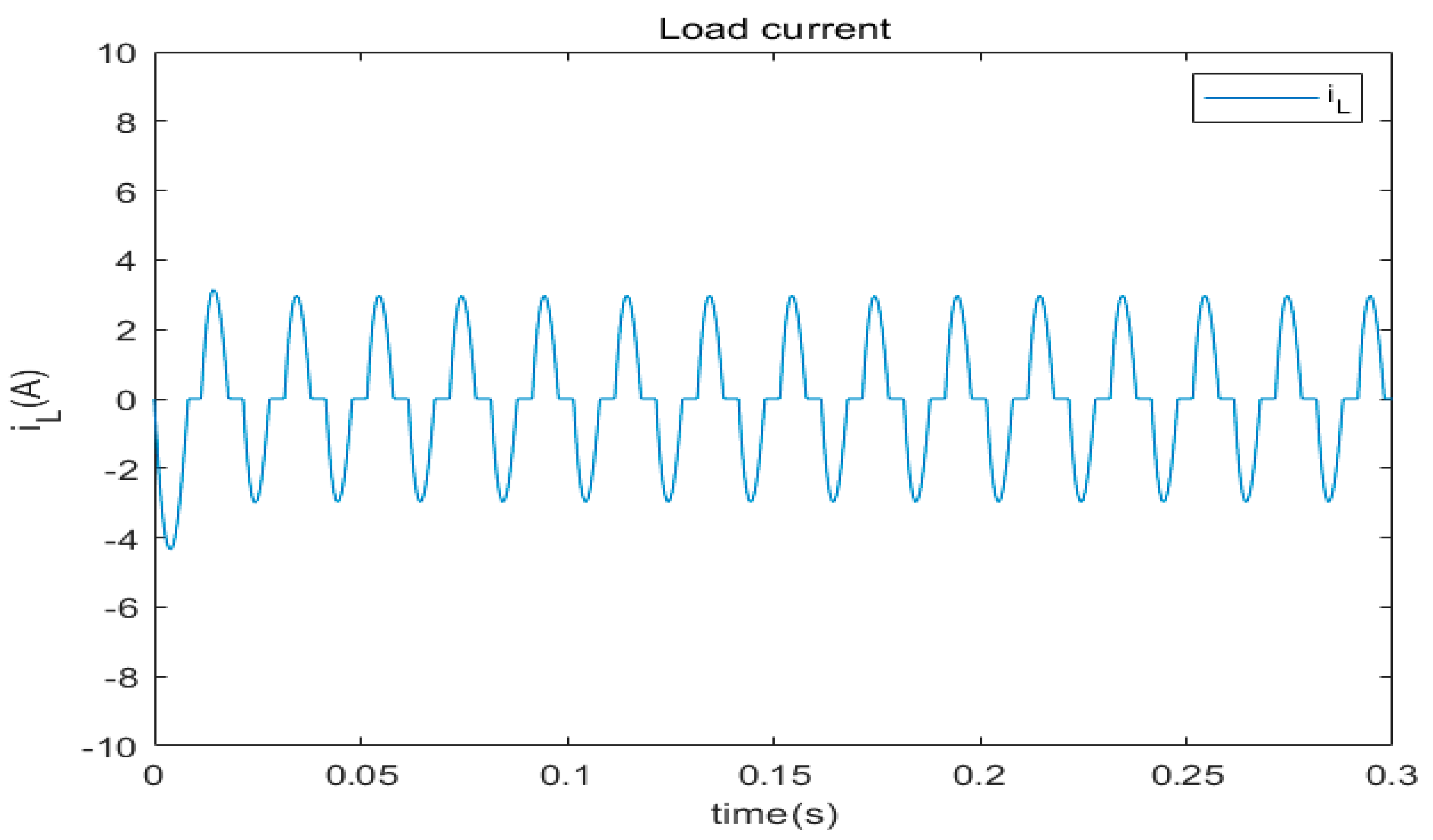
The APF was incorporated into the system at 0 s in the simulation. The curve of load current is shown in
Figure 7, which can also be seen as the power supply current before compensation. By observing the curve of load current, it is not hard to find that the nonlinear load led to severe current distortion, displaying a completely non-sinusoidal periodic waveform. The current of such a waveform will cause great harmonic pollution to the power grid once it flows into the power grid and result in various faults. The power supply current curve shown in
Figure 8 indicates that due to the connection of APF, the supply current became a sinusoidal waveform instead of distortion and the harmonic current was compensated in a very short period of time, which meant the success of compensation task.
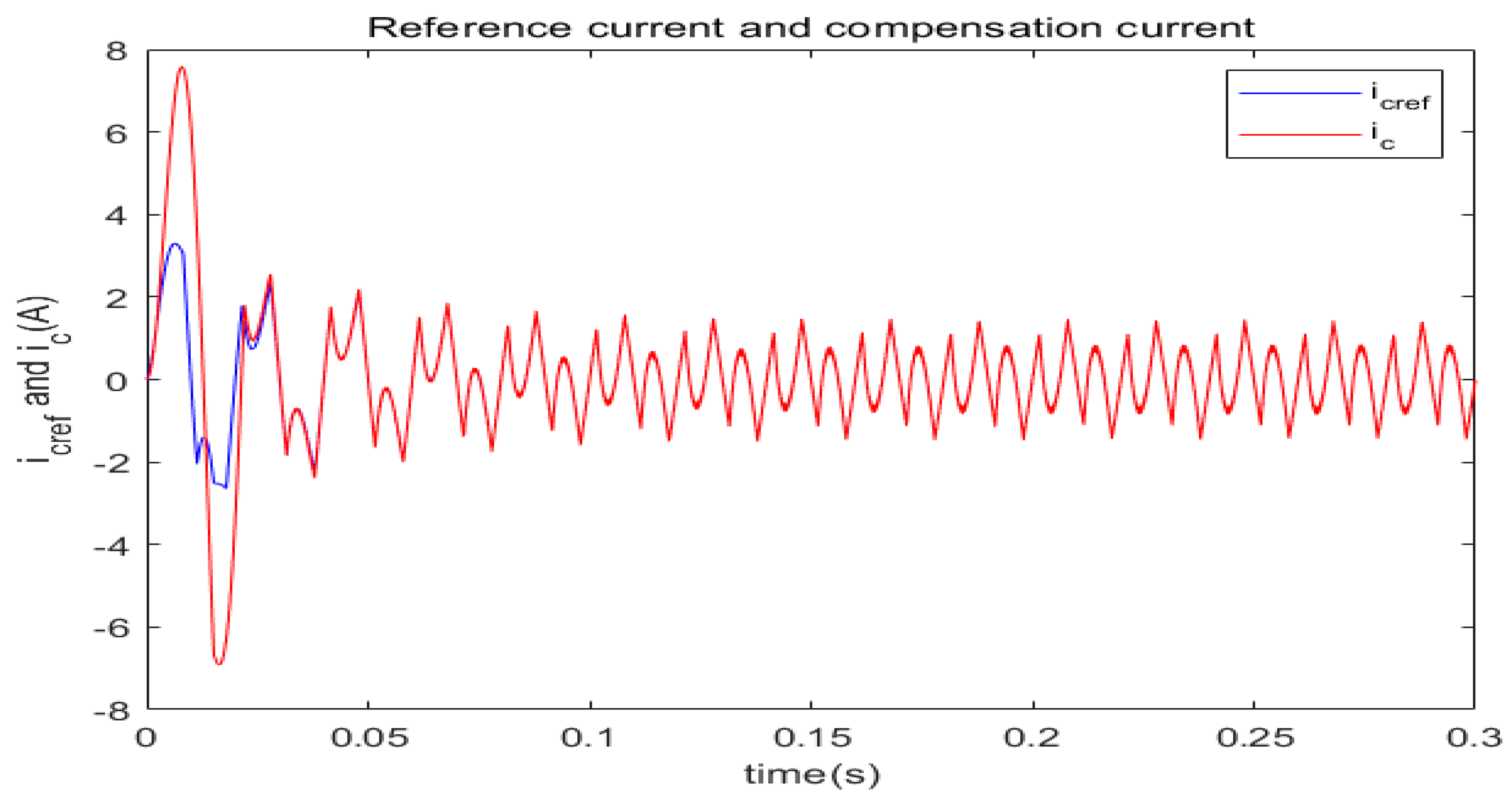
As is illustrated in
Figure 9, the blue curve is the reference current and the red curve is the compensation current output. From the comparison figure, the output compensation current tracked the reference current within 0.03 s on the whole, which indicates a prompt tracking response was achieved. Moreover,
Figure 10 clearly clarifies the error current curve between the reference current and the compensation current under steady-state response. The error current converging to zero after 0.1 s indicates the harmonic compensation was completed.
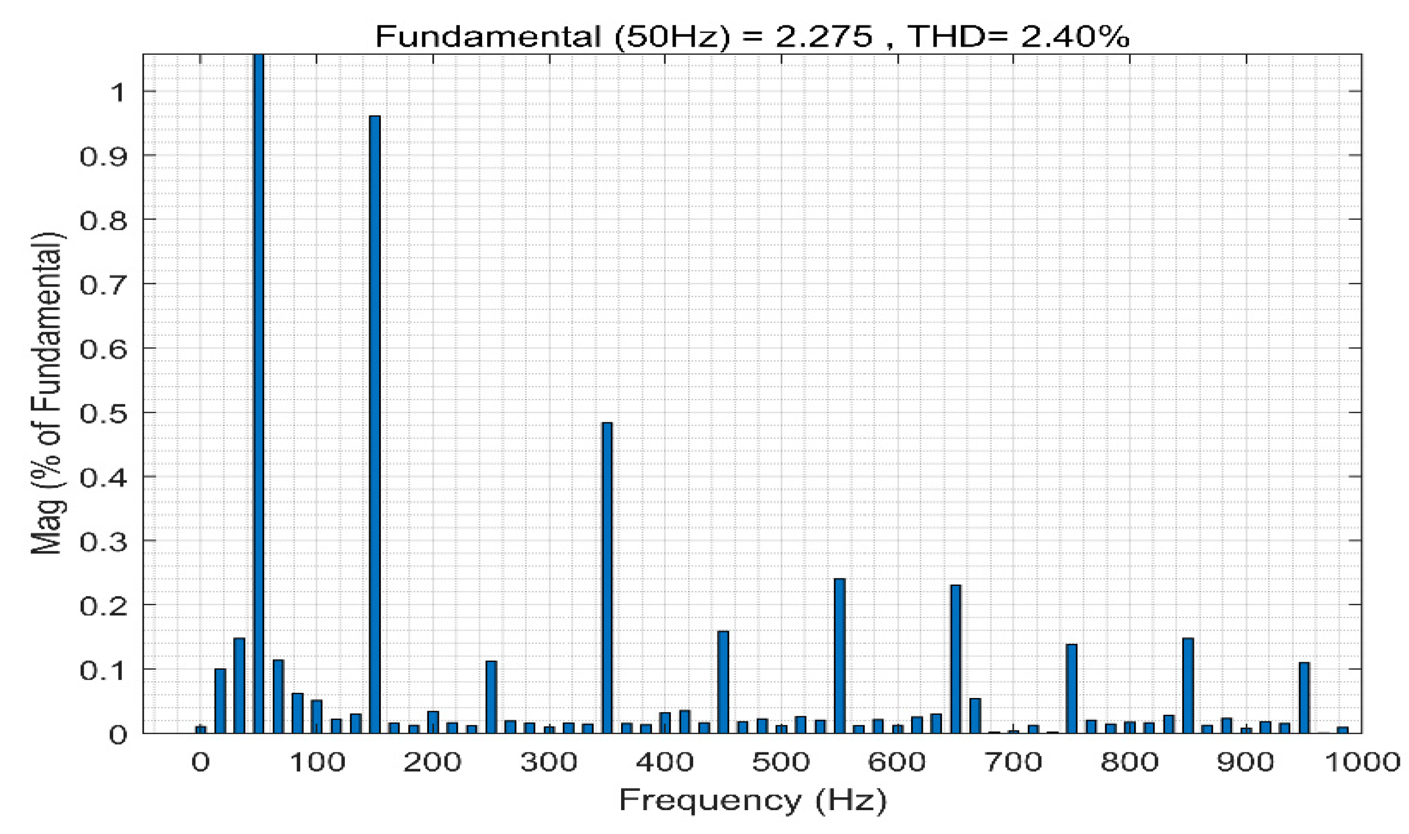
Remark 2. Total harmonic distortion (THD) refers to the sum of the harmonic component in the output signal that is more than the input signal, which is caused by the incomplete linearity of the system; hence, THD is a significant index to evaluate the power quality. THD can be calculated as follows:
whereis the effective value of total current,is the effective value of fundamental wave current, andis the effective value of harmonic components. According to Equation (45),
Figure 11 and
Figure 12 clearly clarify the THD of the power supply current under a steady-state response before and after compensation. Before the connection of APF, the THD of power supply current was high up to 40.3%. A current with such a high content of harmonic components will reduce the efficiency of the production, transmission, and utilization of electricity, resulting in the electrical equipment producing the vibration and noise, overheating, and thus accelerating the aging of the insulating layer. However, after compensation, the THD of the power supply current could be down to 2.4%, far lower than the international standard 5%, which shows the excellent compensation performance of APF.
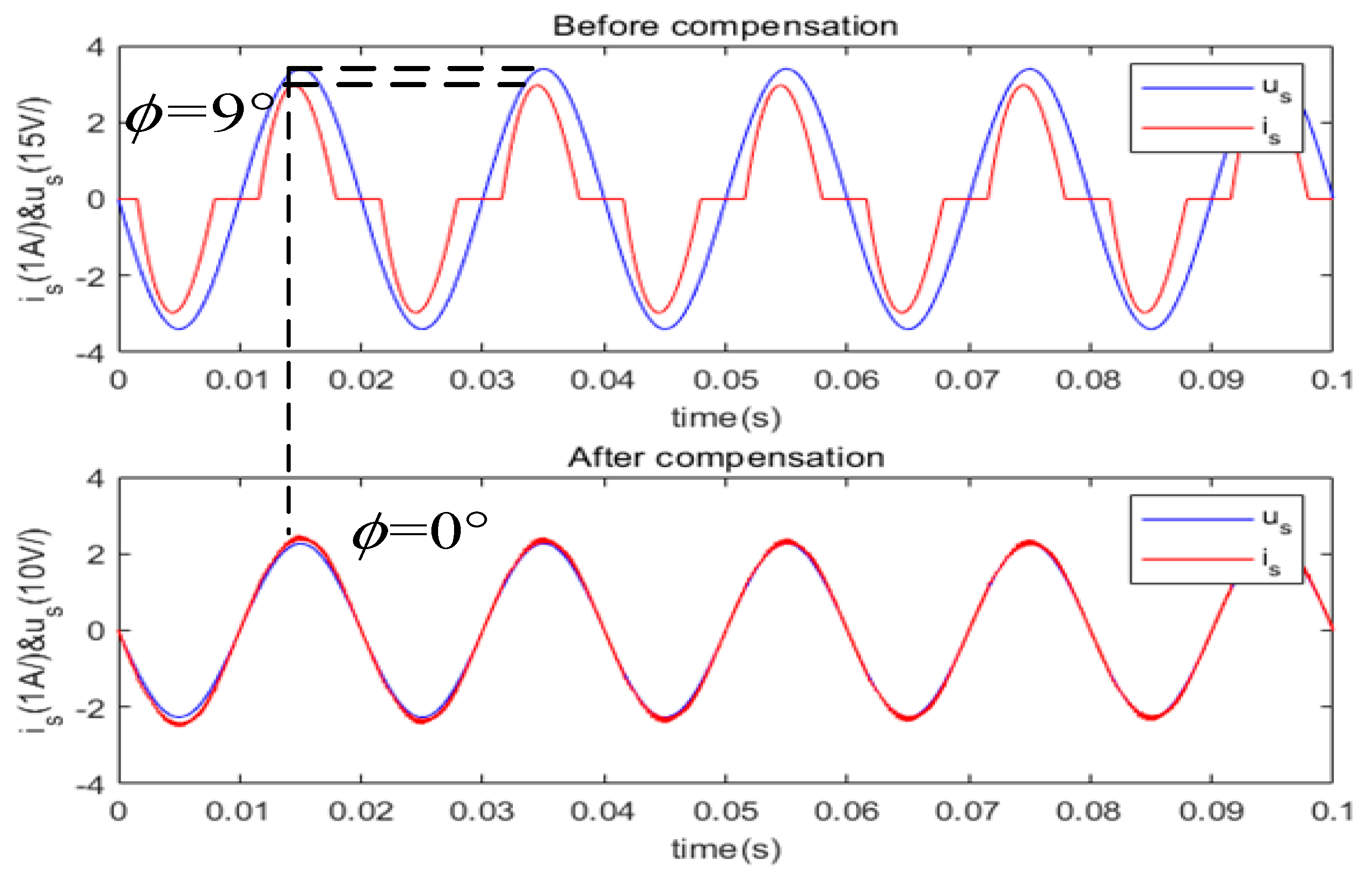
Except compensating harmonics from the nonlinear load, APF can compensate the reactive power on the load side as well; thus, the general evaluation index was comprised of two parts: power factor (PF) and THD. PF is defined as the ratio of active power of AC circuit to apparent power, which is also relevant to the harmonic content in current and the fundamental wave displacement angle. The calculation rule of PF is described as:
where
represents the PF, and
represents the phase angle between voltage and fundamental current, which can be also described as the fundamental current wave displacement angle.
Therefore, the reactive power compensation effect can be judged by calculating the PF from Equation (46). As is shown in
Figure 13, the displacement angle between the power supply voltage wave and fundamental current wave was 9° before compensation. Therefore, the PF was calculated as about 0.9161, which meant that the nonlinear load absorbed a certain amount of reactive power from the system. However, after the connection of APF, the curves of the scaled power supply voltage wave and fundamental current wave almost overlapped and PF was calculated as 0.9997. The lift of PF after the connection of APF gave us a vivid insight that APF had the capacity of not only compensating the harmonics caused by the nonlinear load, but also compensating the reactive power.
- B.
Dynamic Simulation Results and Analysis
A dynamic experiment was carried out on the proposed GFTSMC-NRFNN for the purpose of verifying the effectiveness of the proposed method. A parallel nonlinear load which was composed of an uncontrollable rectifier bridge resistive and capacitive load given in
Table 1 was added at 0.3 s and was removed at 0.6 s.
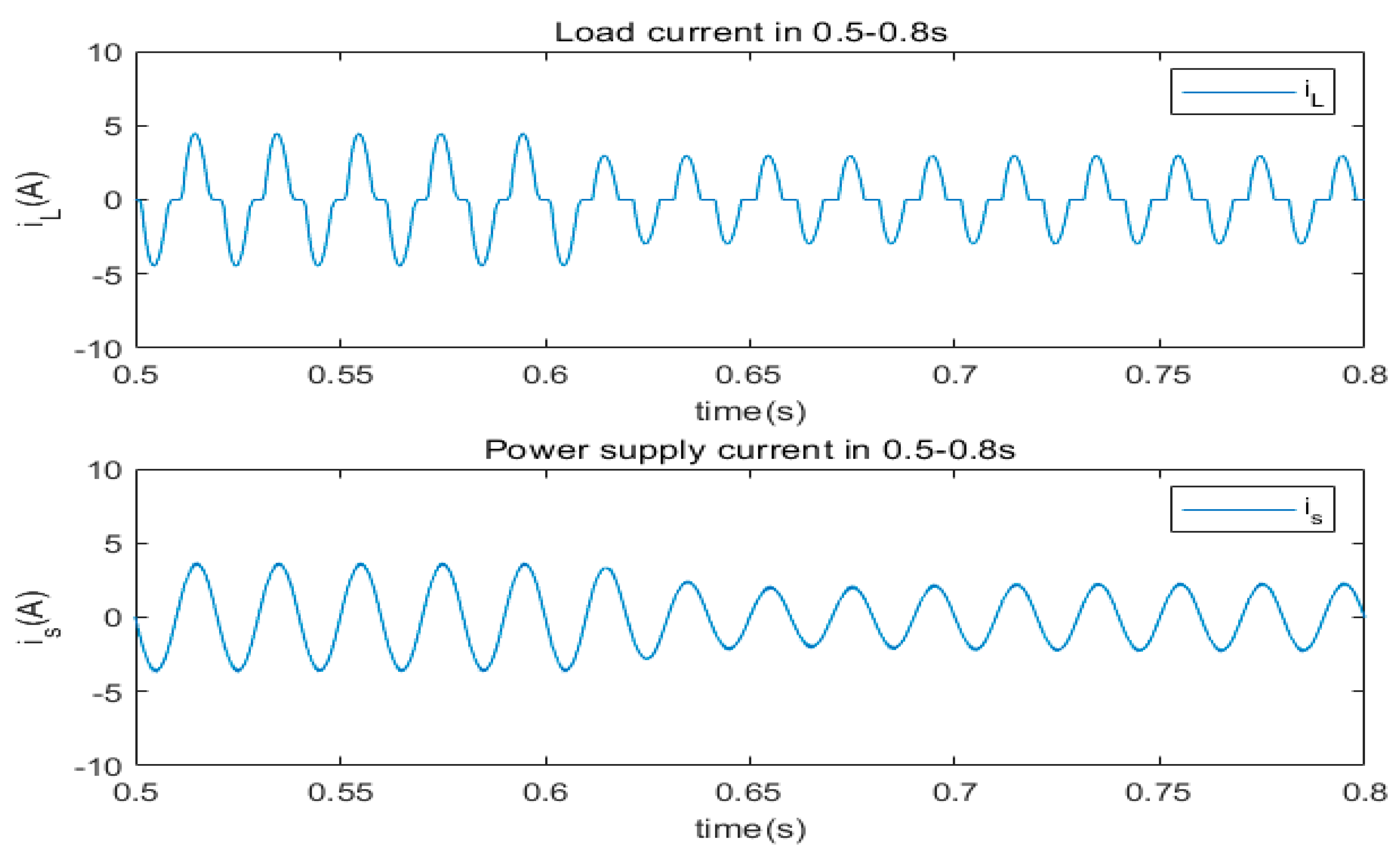
As is vividly depicted in
Figure 14, after the parallel nonlinear load was added at 0.3 s, both the load current and the power supply current had a sudden change and their amplitudes increased. In spite of the sudden change at 0.3 s, the waveform of power supply current quickly returned to a standard sine wave within only two cycles and re-entered a new steady state, implying that the proposed GFTSMC-NRFNN had an excellent dynamic performance. Similarly,
Figure 15 shows the load current and power supply current curve under a dynamic response when the load was decreased at 0.6 s. When the parallel nonlinear load was removed at 0.6 s, the amplitudes of load current and power supply current had a sudden apparent decline. Likewise, the power supply current was able to re-enter a new steady state swiftly.
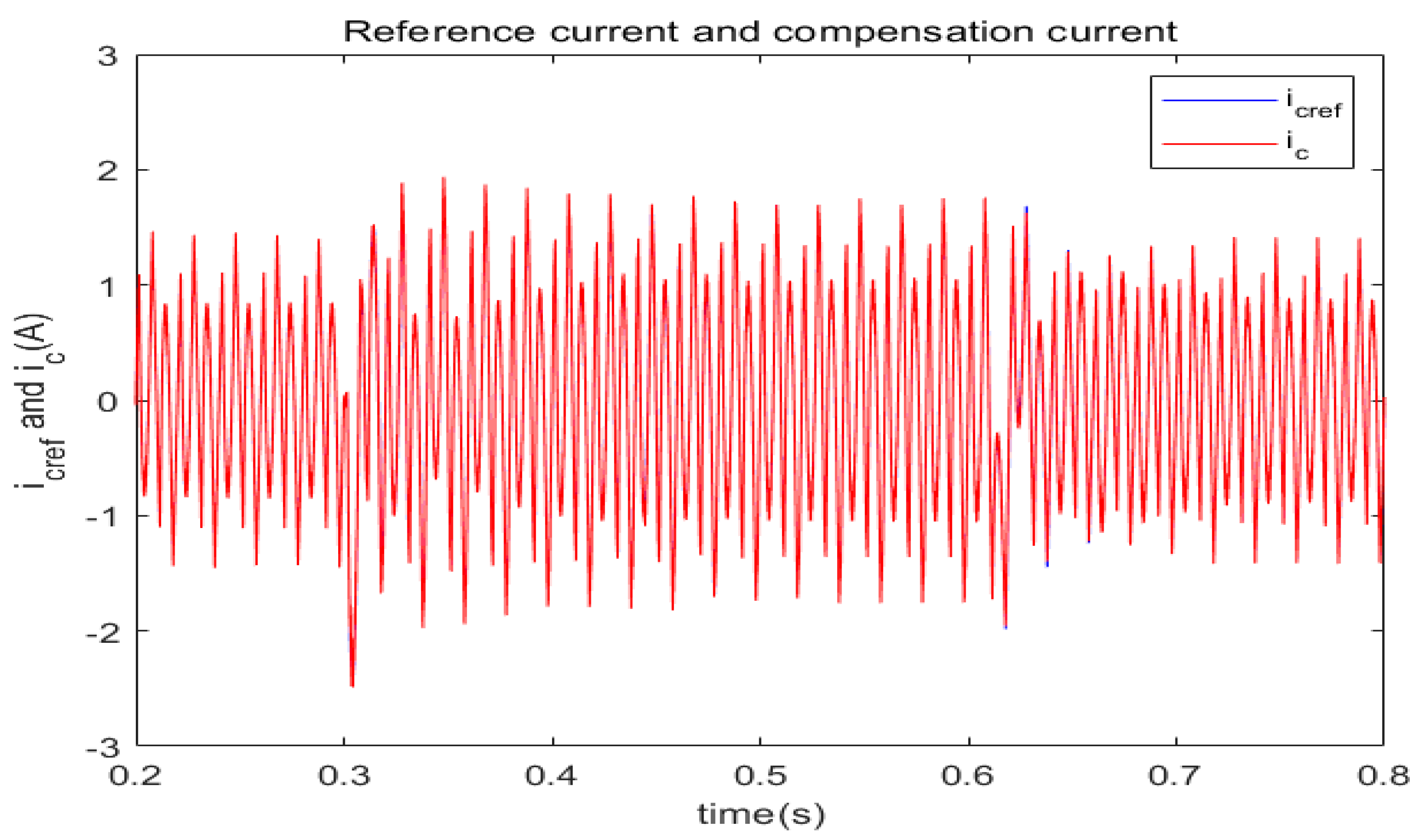
Figure 16 plots the comparison between the reference and compensation current curve of the dynamic response. The blue line represents the reference current, and the red line represents the compensation current. In
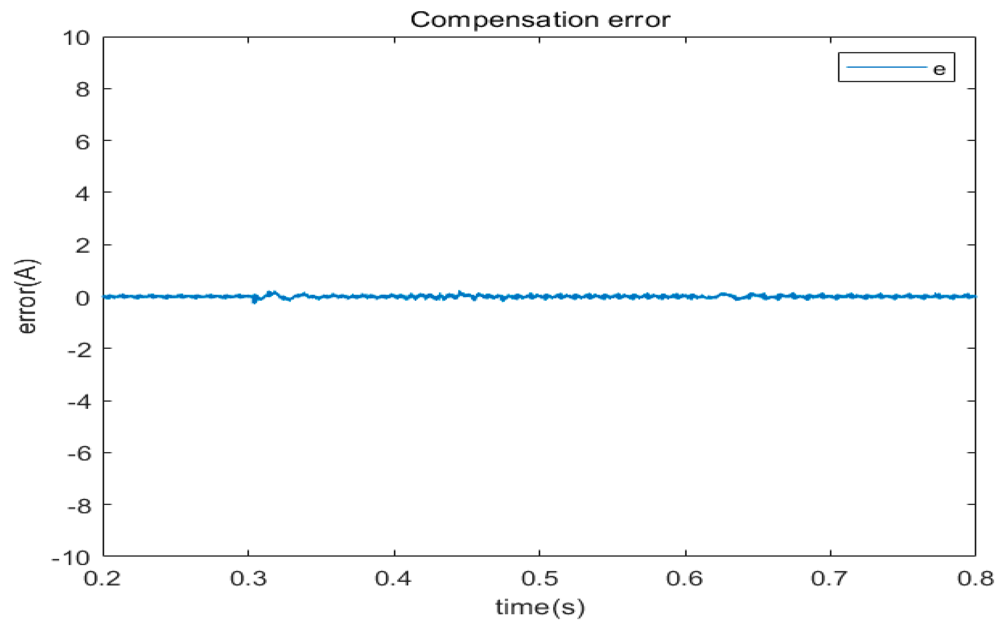
Figure 16, the curve of compensation current basically overlapped the reference current, showing that in the process of dynamic response, however the load changes, the compensation current has the capacity of tracking the reference current promptly and accurately. The error between reference and compensation current is plotted in
Figure 17. In spite of chattering, the error was always kept in a small bounded range. Though the error became larger when the load was increased or decreased, the error was able to re-converge to the equilibrium state again in a short time.
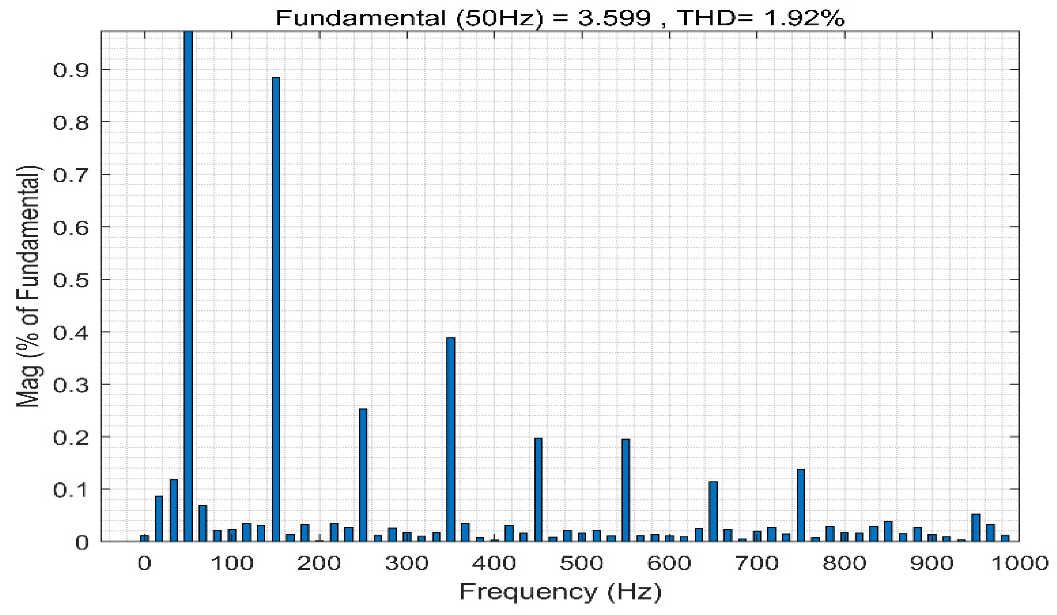
Figure 18 indicates the spectrum of power supply current after the load was increased and the power supply current re-entered into a new steady state. The THD rate was only 1.92%, showing the excellent dynamic compensation performance of APF when the parallel load was suddenly added. Similarly, the THD rate of power supply current in
Figure 19 showing the fantastic dynamic performance of APF when the sudden parallel load was removed was 2.58%.
- C.
Simulation Comparison Results and Analysis
Finally, in order to verify the superiority of the proposed method compared with other methods, a comparison simulation with the traditional SMC of APF based on traditional fuzzy neural network was implemented. The comparison method is abbreviated as SMC-FNN and the proposed method is abbreviated as GFTSMC-NRFNN. For the fairness of the comparison, optimal parameters were selected for the SMC-FNN controller.
According to
Figure 20, which plots the current tracking comparison curve between GFTSMC-NRFNN and SMC-FNN, the compensation current of both methods could track the reference current when entering the steady state. The partial enlargement figures in
Figure 20 imply that when encountering the sudden change of parallel nonlinear load, the compensation current of SMC-FNN was unable to track the reference current promptly and there was tracking misalignment, which was caused by its inability to compensate for the unknown disturbances. The reason why the tracking misalignment of SMC-FNN exists is that the adoption of internal feedback enables the fuzzy neural network to store more information, so as to improve the accuracy of compensation current control. Therefore, compared with SMC-FNN, the proposed GFTSMC-NRFNN had a better dynamic performance.
Furthermore,
Figure 21 shows the error current of two methods under both steady state response and dynamic response. From the first partial enlargement figure, the error of GFTSMC-NRFNN was capable of converging to zero about 0.01 s faster than SMC-FNN, which can be explained due to the fact that the convergence speed of GFTSMC was faster than SMC due to the addition of a nonlinear item. Similarly, the second partial enlargement figure indicates that when the nonlinear load was increased, the compensation error of SMC-FNN was larger than that of GFTSMC-NRFNN and the convergence speed of SMC-FNN was slower.
Table 2 presents the THD data of two strategies under different conditions. At a steady state, the THD of SMC-FNN was 2.57%, which was 1.57% higher than that of GFTSMC-NRFNN. In addition, after the parallel nonlinear load was added, the THD of SMC-FNN was 1.96%, which was 0.04% higher than that of proposed strategy. Moreover, after the parallel nonlinear load was removed, the THD of the compared method was 2.6%, which was 0.02% higher than that of the proposed method. In summary, no matter what the condition was, the THD of GFTSMC-NRFNN was always lower than that of SMC-FNN.
Above all, from the numerical simulation results, the proposed GFTSMC-NRFNN had a better steady-state and dynamic performance than the SMC-FNN, which shows the superiority of the proposed strategy.
Furthermore, in order to present the novelty and superiority of the proposed method over the existing schemes, a comparison was made over the existing methods. Listed in
Table 3 is the comparison THD results of two compared methods such as fuzzy sliding mode control based on adaptive backstepping fuzzy neural network (FSMC-ABFNN) [
16] and dynamic terminal sliding mode control based on double hidden layer recurrent neural network (DTSMC-DHLRNN) [
27] under steady state. The comparison results indicate that the proposed GFTSMC-NRFNN performed better than FSMC-ABFNN and DTSMC-DHLRNN in the numerical simulation.


