Article

Complex Fractional-Order LQIR for Inverted-Pendulum-Type Robotic Mechanisms: Design and Experimental Validation

1
Department of Electrical Engineering, National University of Computer and Emerging Sciences, Lahore 54770, Pakistan
2
Centre for Continuous Manufacturing and Advanced Crystallization, University of Strathclyde, Glasgow G1 1XQ, UK
3
School of Computer Science, Faculty of Science and Engineering, University of Hull, Hull HU6 7RX, UK
*
Author to whom correspondence should be addressed.
Mathematics 2023, 11(4), 913; https://doi.org/10.3390/math11040913
Submission received: 17 January 2023 / Revised: 4 February 2023 / Accepted: 7 February 2023 / Published: 10 February 2023
(This article belongs to the Special Issue Control Theory and Applications)

Abstract

:
This article presents a systematic approach to formulate and experimentally validate a novel Complex Fractional Order (CFO) Linear Quadratic Integral Regulator (LQIR) design to enhance the robustness of inverted-pendulum-type robotic mechanisms against bounded exogenous disturbances. The CFO controllers, an enhanced variant of the conventional fractional-order controllers, are realised by assigning pre-calibrated complex numbers to the order of the integral and differential operators in the control law. This arrangement significantly improves the structural flexibility of the control law, and hence, subsequently strengthens its robustness against the parametric uncertainties and nonlinear disturbances encountered by the aforementioned under-actuated system. The proposed control procedure uses the ubiquitous LQIR as the baseline controller that is augmented with CFO differential and integral operators. The fractional complex orders in LQIR are calibrated offline by minimising an objective function that aims at attenuating the position-regulation error while economising the control activity. The effectiveness of the CFO-LQIR is benchmarked against its integer and fractional-order counterparts. The ability of each controller to mitigate the disturbances in inverted-pendulum-type robotic systems is rigorously tested by conducting real-time experiments on Quanser single-link rotary pendulum system. The experimental outcomes validate the superior disturbance rejection capability of the CFO-LQIR by yielding rapid transits and strong damping against disturbances while preserving the control input economy and closed-loop stability of the system.

1. Introduction

Inverted-pendulum-type robots are widely favoured as a benchmark platform to examine and verify the advanced control methods designed to regulate the behaviour of under-actuated nonlinear systems [1]. The principles of inverted pendulum stabilisation are extensively used in the development of robust balancing control systems for legged humanoid robots, two-wheeled transporters, drones, aerial robots, submarine vessels, satellites, missiles, rockets, etc. [2]. Robot designs based on the inverted-pendulum require fewer actuators for motion control, which results in better control-input efficiency, higher dexterity, and a lesser propensity to break down [3].
Balance control and disturbance rejection are two important requirements for these systems in real-time applications, and methodically addressing them is not trivial [4]. In every application of Inverted Pendulum (IP) systems, a well-postulated balancing controller is a prerequisite that enables a robot to stabilise its posture in a structured environment [5]. Formulating an agile controller for a complex dynamical system is a difficult task indeed [6]. With fewer actuators than the degrees of freedom to be regulated, these systems represent an under-actuated behaviour [7]. Apart from their under-actuated configuration, these systems pose open-loop kinematic instability, highly nonlinear dynamics, and chaotic behaviour [8]. Furthermore, the system’s performance is prone to being affected by random disturbances imparted by environmental indeterminacies [9]. Due to the aforementioned nonlinear characteristics, controlling such systems becomes much harder under the influence of exogenous disturbances, transients, parametric uncertainties, and varying loads [10]. Therefore, there is a dire need for formulating robust and stable closed-loop controllers that yield fast response speeds and strong disturbance compensation behaviour [11].
Proportional–Integral–Derivative controllers are reasonably simple to construct, and they offer a reliable control yield for IP systems [12]. However, their linear configuration lacks the necessary degrees of freedom to effectively compensate for nonlinear disturbances [13]. Moreover, the fixed gains of these pre-designed controllers lack the flexibility to address slight variations in the operating conditions or parametric uncertainties [14]. Sliding mode controllers are conventionally used to deliver robust control effort to balance IP systems [15]. They generate highly discontinuous control activity and impose large input requirements that induce chattering in the response [16]. Fuzzy controllers yield agile balance control decisions for IP-type robot systems due to their flexible design [17]. However, synthesising the aforementioned intelligent controllers requires a well-calibrated rule base and large training data sets that increase the computational expense [18]. The Linear–Quadratic Regulator (LQR) is considered the most dominant model-based linear controller for the proposed IP-type robotic systems [19]. However, its yield gets severely degraded under the influence of unprecedented model variations, identification errors, and random noise, which generally lead to the complete collapse of the IP system [20]. Hence, the utilisation of the ubiquitous LQR is considered ill suited for controlling nonlinear IP-type under-actuated systems under disturbances [21].
The limited degrees of freedom of the PID controller, the fragile robustness of the LQR, the discontinuous control activity of SMC, and the computational complexity of intelligent controllers to regulate IP systems can be addressed by employing fractional-order controllers [22]. Fractional calculus has been extensively used in the scientific literature to accurately model and control complex and nonlinear dynamical systems [23]. Fractional-Order (FO) control, a well-known application area of fractional calculus, introduces control laws that involve fractional-ordered integration and differentiation operators [24]. The new parameters introduced in the form of the fractional orders of the aforementioned operators increase the controller’s design flexibility, which allows the control law to efficiently compensate for exogenous disturbances [25]. The fractional order of the mentioned operators can be selected as real, complex, or variable, depending on the system’s requirement [26]. Fractional-order controllers have also been applied to regulate the behaviour of IP-type nonlinear systems [27].
The extension of conventional FO controllers to formulate Complex Fractional-Order (CFO) controllers has recently gained a lot of attraction [28]. These controllers are designed such that the real-numbered fractional orders of differentiation/integration operators of the control law are replaced with complex orders of the form z = c + j d , where z is a complex number, and c and d represent the coefficients of the real and imaginary parts, respectively [29]. The shortcomings associated with the aforementioned controllers can be addressed by using fraction-order controllers. The augmentation of the differentiation/integration operators with a well-calibrated imaginary order undertakes to further improve the design flexibility of the control law, which significantly enhances the controller’s disturbance rejection capability and robustness against parametric uncertainties [30]. The complex orders further increase the controller’s degrees of freedom, thus allowing it to better address the exogenous perturbations while preserving the control efficiency. The utilisation of CFO controllers has recently gained a lot of attraction in various modern applications [30,31]. Scientific studies justify the usage of CFO controllers to deliver rapid transits with relatively stronger damping against disturbances for real-world engineering systems [32]. Thus, as compared to the aforementioned conventional control schemes, the CFO procedure offers favourable control behaviour across a broad range of operating conditions.
This article mainly contributes to systematically designing and experimentally validating an innovative CFO state feedback controller to improve the disturbance rejection capability and response speed of the nonlinear and under-actuated inverted-pendulum-type robotic mechanisms. The proposed control procedure employs the Linear–Quadratic–Integral Regulator (LQIR) as the baseline integer-order controller for the rotary inverted pendulum. The standard rotary inverted pendulum is chosen as the benchmarking experimental platform in this research due to its nonlinear dynamics, kinematic instability, and under-actuated characteristics [33]. The novel contributions of this research work are highlighted as follows:
  • Firstly, the differential/integral operators of the baseline controller are retrofitted with pre-calibrated real-numbered fractional-order operators to develop an FO-LQIR.
  • The FO-LQIR is systematically extended to a CFO-LQIR to robustify the control law’s performance. This is achieved by replacing the real-numbered fractional order of each operator in the control law with pre-configured complex-order operators. The new parameters introduced in each control law are empirically tuned by iteratively minimising a quadratic objective function that considers the position regulation errors and control input energy.
  • The efficacies and benefits of the proposed CFO-LQIR are benchmarked against the integer-order LQIR and FO-LQIR by conducting credible real-time hardware experiments on the Quanser single-link rotary pendulum setup [25].
The proposed CFO controller offers several benefits. It is evident from the scientific literature that FO controllers demonstrate better robustness and stabilisation control capabilities than their integer-order counterparts for rotary pendulums and other (similar) self-balancing robotic applications [25,26]. This establishes a clear motivation to methodically transform the ubiquitous FO controller into the proposed CFO controller for the rotary pendulum system to achieve superior robustness against disturbances and uncertainties. Furthermore, CFO controllers specialise in effectively handling the highly nonlinear, chaotic, and time-varying dynamics of complex higher-order systems. Inverted-pendulum-type robotic systems present all the aforementioned properties. Therefore, this is another major reason for formulating the CFO-LQIR to address the nonlinear control problem in this research. Although there have been some research works simulating the idea proposed in this paper [28,29], to the best of authors’ knowledge, the experimental validation of this idea has not been thoroughly reported as of today in the available literature. This essentially lays down the novelty and originality of the proposed research.
The remaining paper is organised as follows. The system’s dynamic model is derived in Section 2. The development of the baseline integer-order LQIR is presented in Section 3. Section 4 discusses the FO-LQIR design, and the proposed CFO-LQIR is formulated in Section 5. Experimental results are analysed and discussed in Section 6. Finally, Section 7 concludes this research.

2. System Description

The Single Rotary Inverted Pendulum (SRIP) is a well-known self-balancing electro-mechanical system with nonlinear dynamics and an under-actuated configuration. It has a single link that needs to be stabilised vertically. The aforementioned characteristics make the SRIP an ideal candidate platform to experimentally investigate and validate the efficacies of the proposed control laws for self-balancing robotic systems. The hardware schematic of a standard rotary pendulum is illustrated in Figure 1. The setup consists of a motorised horizontal rotating arm that generates the necessary energy to swing up and vertically balance the apparatus rod connected to it. The arm is rotated with the aid of a DC-geared servo motor that is coupled to one end of the arm link. The arm’s angular displacement ( α ) is measured via a rotary encoder that is installed with the motor’s shaft. The free end of the arm is attached to the apparatus rod that rotates freely about its pivot. The rod’s angular displacement ( θ ) is measured via another encoder that is commissioned at its pivot.
The system’s dynamic model is derived in terms of its generalised coordinates, α and θ , by using the Euler–Lagrange technique [34]. The system’s Lagrangian ( L ( t ) ) is evaluated as the difference between the system’s total potential energy ( E P ( t ) ) and kinetic energy ( E K ( t ) ), as given in (1), [15].
L ( t ) = E K ( t ) E P ( t )  
where
E P ( t ) = M p l p g ( cos θ ( t ) ) ,   E K ( t ) = 1 2 J e ( α ˙ ( t ) ) 2 + 1 2 M p ( r α ˙ ( t ) l p θ ˙ ( t ) ( cos θ ( t ) ) ) 2 + 1 2 M p ( l p θ ˙ ( t ) ( sin θ ( t ) ) ) 2 + 1 2 J p ( θ ˙ ( t ) ) 2
The model parameters are identified in Table 1. The Lagrangian is given as
L ( t ) = 1 2 ( J e + M p r 2 ) ( α ˙ ( t ) ) 2 + ( 2 3 M p l p 2 + 1 2 J p ) ( θ ˙ ( t ) ) 2 M p l p r ( cos θ ( t ) ) α ˙ ( t ) θ ˙ ( t ) M p l p g ( cos θ ( t ) )  
The nonlinear equations of motion are acquired using the following expressions [34].
δ δ t ( δ L δ α ˙ ) δ L δ α = τ b v α ˙ ( t ) ,     δ δ t ( δ L δ θ ˙ ) δ L δ θ = 0  
where τ ( t ) is the motor control torque, and b v represents the viscous friction in the motor. The value of b v is negligible. The motor torque is expressed as follows.
τ ( t ) = K t ( V m ( t ) K m α ˙ ( t ) ) R m    
where V m ( t ) is the motor’s voltage. The solution leads to the following equations.
α ¨ ( t ) = r M p 2 l p 2 g ( cos θ ( t ) ) θ ( t ) J p M p r 2 cos θ ( t ) sin θ ( t ) ( α ˙ ( t ) ) 2 ( J p + M p l p 2 ) τ ( t ) ( M p r 2 ( sin 2 θ ( t ) ) J e M p r 2 ) J p M p l p 2 J e
θ ¨ ( t ) = M p l p ( ( M p r 2 g ( sin 2 θ ( t ) ) J e g M p r 2 g ) θ ( t ) + r J e sin θ ( t ) ( α ˙ ( t ) ) 2 r τ ( t ) cos θ ( t ) ) ( M p r 2 ( sin 2 θ ( t ) ) J e M p r 2 ) J p M p l p 2 J e  
where α ( t ) and θ ( t ) represent the angular positions of the arm and the rod, respectively, α ˙ ( t ) and θ ˙ ( t ) are the angular velocities of the arm and the rod, respectively, and α ¨ ( t ) and θ ¨ ( t ) are the angular accelerations of the arm and the rod, respectively.
The system’s model is linearised about the vertical position, where α ( t ) = π   rad . ,   θ ( t ) = 0 ,   α ˙ ( t ) = 0 ,   θ ˙ ( t ) = 0 . The small angular displacements are approximated such that sin θ ( t ) 0 and cos θ ( t ) 1 . These approximations yield the following linearised state equations.
α ¨ ( t ) = 1 H ( r M p 2 l p 2 g θ ( t ) ( J p + M p l p 2 ) K t K m R m α ˙ ( t ) + ( J p + M p l p 2 ) K t R m V m ( t ) )
θ ¨ ( t ) = 1 H ( M p l p g ( J e + M p r 2 ) θ ( t ) r M p l p K t K m R m α ˙ ( t ) + r M p l p K t R m V m ( t ) )      
such   that  
H = J e J p + M p r 2 J p + M p l p 2 J e
The state-space representation of linear dynamical systems is expressed as
x ˙ ( t ) = A x ( t ) + B u ( t ) ,     y ( t ) = C x ( t ) + D u ( t )
where x ( t ) is the state vector, y ( t ) is the output vector, u ( t ) is the control input signal, A is the system matrix, B is the input matrix, C is the output matrix, and D is the feed-forward matrix. The system’s state and input vectors are provided in (10) [34].
x ( t ) = [ α ( t ) θ ( t ) α ˙ ( t ) θ ˙ ( t ) ] T , u ( t ) = V m ( t )
The nominal linear state-space model of the SRIP is given by (11) [15].
A = [ 0 0 1     0 0 0 0     1 0 a 1 a 2 0 0 a 3 a 4 0 ] , B = [ 0 0 b 1 b 2 ] , C = [ 1 0 0 0 0 1 0 0 0 0 1 0 0 0 0 1 ] , D = [ 0 0 0 0 ]  
where
a 1 = r M p 2 l p 2 g J p J e + J e l p 2 M p + J p M p r 2 , a 2 = K t K m ( J p + M p l p 2 ) ( J p J e + J e l p 2 M p + J p M p r 2 ) R m , a 3 = M p l p g ( J e + M p r 2 ) J p J e + J e l p 2 M p + J p M p r 2 , a 4 = r M p l p K t K m ( J p J e + J e l p 2 M p + J p M p r 2 ) R m , b 1 = K t ( J p + M p l p 2 ) ( J p J e + J e l p 2 M p + J p M p r 2 ) R m , b 2 = r M p l p K t ( J p J e + J e l p 2 M p + J p M p r 2 ) R m
The model parameters of the rotary pendulum are identified in Table 1 [35].

3. Linear–Quadratic–Integral Regulator (LQIR)

In this research, the LQIR is adopted as the baseline integer-order state compensator to vertically stabilise the pendulum rod and to regulate the arm at its reference position while preserving the system’s closed-loop asymptotic stability.

3.1. LQIR Formulation

The LQR is designed by minimising a Quadratic Performance Index (QPI) of the state and control input variables [36]. The Hamilton–Jacobi–Bellman (HJB) equations are solved to minimise the total cost and to deliver an optimal state compensator offline [37]. The QPI used in this research is given as
J l q = 1 2 0 ( x ( t ) T Q x ( t ) + u ( t ) T R u ( t ) ) d t
where Q 4×4 is a user-specified positive semi-definite state weighting matrix, and R ℝ is a user-specified positive definite input weighting matrix. The Q and R matrices penalise the system’s state and control input variations, respectively. These matrices are symbolically represented as
Q = diag ( q α q θ q α ˙ q θ ˙ ) , R = ρ
where q x 0 and ρ > 0 represent the real-numbered coefficients of the respective matrices. The value of ρ is preset to unity to ensure an economical control activity. The coefficients of the 𝑸 matrix are carefully calibrated offline by using the tuning procedure discussed in the following subsection. The optimised 𝑸 and 𝑹 matrices are used with the Riccati Equation, as expressed in (14), to compute its solution 𝑷.
A T P + P A P B R 1 B T P + Q = 0
where P   4×4 is a symmetric positive definite matrix. The matrix P is used to calculate the state compensator gain vector K , as shown below.
K = R 1 B T P
where K = [ k α k θ k α ˙ k θ ˙ ] . The conventional LQR law is expressed as follows.
u l q r ( t ) = K x ( t )
The following Lyapunov function is used to prove the asymptotic stability of the control law [36].
M ( t ) = x ( t ) T P ( t ) x ( t ) > 0 ,           for   x ( t ) 0        
The first derivative of the Lyapunov function is expressed as follows.
  M ˙ ( t ) = 2 x ( t ) T P x ˙ ( t ) = 2 x ( t ) T P ( A B K ( t ) ) x ( t )     = 2 x ( t ) T P ( A B R 1 B T P ) x ( t )                                                                                           = x ( t ) T ( P A + A T P ) x ( t ) 2 x ( t ) T ( P B R 1 B T P ) x ( t )          
By substituting Equation (14), the derivative M ˙ ( t ) simplifies, as given in (19).
M ˙ ( t ) = x ( t ) T Q ¯ x ( t ) x ( t ) T ( P B R 1 B T P ) x ( t )     < 0          
The expression of M ˙ ( t ) is negative semi-definite as long as Q = Q T 0 and R = R T > 0 . This condition is sufficient to guarantee the closed-loop asymptotic stability of the LQR law.
To increase the controller’s degrees of freedom, the conventional LQR is retrofitted with an auxiliary integral controller that enhances the system’s reference-tracking accuracy and damping strength against position regulation errors. The integral controller is expressed as the weighted sum of the error integral variables, as given in (20).
u I ( t ) = k i α 0 t e α ( τ ) d τ + k i θ 0 t e θ ( τ ) d τ        
such   that
e α ( t ) = α ( 0 ) α ( t ) , e θ ( t ) = π θ ( t )
where e α and e θ represent the error between the actual position and the reference position of the arm and the apparatus rod, respectively, and k i α and k i θ are the pre-calibrated integral gains associated with the respective error integral variables. The tuning procedure used to select the integral gains offline is discussed in the following sub-section. The resulting LQIR law is expressed as the linear combination of the conventional LQR and the aforementioned integral controller.
u ( t ) = u l q r ( t ) + u I ( t )
The LQIR law, in terms of the integer-order differential and integral operators, is expressed in (22).
u ( t ) = k α α ( t ) k θ θ ( t ) k α ˙ α ˙ ( t ) k θ ˙ θ ˙ ( t ) + k i α 0 t e α ( τ ) d τ + k i θ 0 t e θ ( τ ) d τ
The control signal, u ( t ) , is bounded within ± V m a x = ± 18.0   V to avoid over-heating or unnecessary wear and tear of the actuator’s winding [35]. For this purpose, the control signal is subjected to the saturation function, as shown below.
s a t ( u ( t ) ) = { V m a x ,                                                                           u ( t ) V m a x u ( t ) ,                             V m a x < u ( t ) < V m a x V m a x ,                                                                         u ( t ) V m a x                                                                  

3.2. Parameter Tuning Procedure

The LQR design depends upon the system’s state and control input variations, as dictated by J l q . However, assigning appropriate weights to the aforementioned variables is extremely important to ensure an optimal control yield. The trial-and-error-based settings of the Q and R matrices are limited by the designer’s experience and thus may not always deliver accurate position regulation and transient recovery behaviour [38]. Hence, in this section, a new objective function is introduced that considers the control variations as well as the error variations depicted by the time domain responses of α and θ . The cost function is expressed as
J c = 0 ( | e α ( t ) | 2 + | e θ ( t ) | 2 + | u ( t ) | 2 ) d t
Equal weights are set for the constituents of the aforementioned cost function to apply an equal impact to the state error minimisation as well as the control signal minimisation criteria. Applying the same weights to the state error and control input terms tends to deliver a good time domain response while economising the control energy expenditure to prevent actuator saturation [39]. The state-weighting factors are searched within the range [0, 100]. The offline selection process is initiated by giving equal (unity) weight to each state variable, such that Q = diag ( 1 1 1 1 ) . The range space is iteratively explored in the direction of the steepest gradient descent of the aforementioned objective function. In every iteration, the pendulum is allowed to vertically balance, the arm maintains its stations for 10.0 s, and the consequent cost is evaluated. The iterative tuning is terminated only when the minimum cost is achieved. The coefficients of Q and R thus optimised are given as q α = 32.8 , q θ = 52.2 , q α ˙ = 6.1 , q θ ˙ = 2.5 , and ρ = 1 . The application of the optimised set of the Q and R matrices to the Riccati equation delivers the following state compensator gains: k α = 6.21 , k θ = 130.56 , k α ˙ = 4.22 , and k θ ˙ = 17.83 . The integrals’ gains associated with the control law are also tuned by iteratively minimising the objective function using the same procedure, as discussed above. The integral gains are selected from the range [−5, 0]. Consequently, the integral gains calibrated for this research are k i α = 2.06 and k i θ = 7.47 × 10 6 .

4. Fractional-Order LQIR

This section comprehensively presents the constitution of the FO-LQIR law.

4.1. Fractional Calculus

Fractional calculus mainly deals with the integral and differential operators used in mathematical computations by assigning them pre-calibrated fractional powers instead of the typical integer ones [25]. The symbol used to represent the fractional mathematical operator is D λ , where λ is the generalised fractional order of the operator. The capability of fractional calculus to model and control the behaviour of highly chaotic and nonlinear systems is mainly attributed to the non-integer characteristics of the fractional orders that enables it to realise and address the system’s intrinsic un-modeled nonlinearities [40]. The fractional operators are mathematically defined via the well-known definitions given by Riemann–Liouville, Gruunwald–Letnikov, and Caputo [41]. These definitions are described, respectively, in (25)–(27).
D λ f ( t ) = 1 Γ ( n λ ) d n d t n a t f ( τ ) ( t τ ) λ n + 1 d τ
where f ( t ) is an arbitrary function, Γ ( x ) is the Euler gamma function, and n is an integer such that n 1 < λ < n .
D λ f ( t ) = lim h 0 1 h i i = 0 ( t a ) / h ( 1 ) i ( λ i ) f ( t i h )              
where ( λ i ) = Γ ( λ + 1 ) / Γ ( i + 1 ) Γ ( λ i + 1 ) , and h is the step size.
D λ f ( t ) = 1 Γ ( λ n ) a t f n ( τ ) ( t τ ) λ n + 1 d τ          

4.2. Fractional-Order Control Law Formulation

Fractional calculus can be combined with the (typical) integer-order LQIR to transform them into their fractional-order counterpart [42]. Hence, in this research, fractional calculus is used to transform the LQIR law synthesised in Section 3 into its fractional order counterpart. To realise the FO-LQIR law, the baseline LQIR law is augmented with fractional-order operators, as given in (28).
u ( t ) = k α α ( t ) k θ θ ( t ) k α ˙ ( D β α ( t ) ) k θ ˙ ( D γ θ ( t ) ) + k i α ( D δ e α ( t ) ) + k i θ ( D μ e θ ( t ) )  
The control law expressed in (27) uses the six original gains, k α , k θ , k α ˙ , k θ ˙ , k i α , and k i θ , which have already been prescribed in Section 3.2. The control law also introduces four new pre-configured parameters, β , γ , δ , and μ , that serve as the fractional orders of the integral and differential operators. The parameters β and γ are the real-numbered fractional orders associated with the differential operators of α ( t ) and θ ( t ) , respectively. The parameters δ and μ are the real-numbered fractional orders associated with the integral operators of e α ( t ) and e θ ( t ) , respectively. It is well known that the value of the reference signals does not affect the control law design in a typical regulatory control system. Hence, to simplify the computations, it is safe to assume that e α ( t ) = α ( t ) and e θ ( t ) = θ ( t ) . The FO-LQIR law can then be expressed as shown in (29).
u ( t ) = u α ( t ) + u θ ( t )
where
u α ( t ) = k α α ( t ) k α ˙ ( D β α ( t ) ) k i α ( D δ α ( t ) )
and
u θ ( t ) = k θ θ ( t ) k θ ˙ ( D γ θ ( t ) ) k i θ ( D μ θ ( t ) )
The transfer functions of the control laws u α ( t ) and u θ ( t ) are identified in (30).
C α ( s ) = U α ( s ) α ( s ) = k α k α ˙ s β k i α s δ , C θ ( s ) = U θ ( s ) θ ( s ) = k θ k θ ˙ s γ k i θ s μ  
where s is the Laplace operator. The computational implementation of the terms s β , s δ , s γ , and s μ is quite difficult, owing to the fractional orders. Hence, these fractional operators are approximated via the Oustaloup recursive approximation to simplify their digital realisation [43]. The fractional operator s λ can be approximated via the Oustaloup method, as given in (31).
s λ = C i = 1 N 1 + ( s ω z , i ) 1 + ( s ω p , i )      
such that
ω z , i = ω L ( ω H ω L ) 2 i 1 λ 2 N , ω p , i = ω L ( ω H ω L ) 2 i 1 + λ 2 N
where N is the order of the filter, and ω L and ω H are the lower and the upper translational frequencies of the filter, respectively. The value of C is selected such that ( j ω ) λ = 1 at 1.0 rad/s. In this work, a fifth-order Oustaloup recursive filter is employed with ω L = 10 2 rad/s and ω H = 10 2 rad/s to approximate the fractional operators.
The fractional orders associated with the FO-LQIR law are tuned by iteratively minimising the objective function J c using the procedure discussed in Section 3.2. The fractional orders are selected from the range [0, 2]. If the value of the fractional orders converges to zero, the integral/differential operators represent a simple proportional control term, whereas if the value of the fractional orders converges to unity, the operators mutate into the typical integer-order integral/differential control terms. The fractional orders chosen for the FO-LQIR are β = 0.865 , γ = 0.882 , δ = 0.479 , and μ = 0.348 .

5. Complex Fractional-Order LQIR

Complex fractional order controllers are formulated by augmenting the integer-order controllers with integral and differential operators, having complex-numbered orders instead of real-numbered fractional orders. The CFO-LQIR originates from third-generation Commande Robuste d’Ordre Non Entier (CRONE) control [44]. The CFO-LQIR proposed in this section is formulated such that all the integral/differential operators have a complex order, as given in (32).
u ( t ) = k α α ( t ) k θ θ ( t ) k α ˙ ( D d α ( t ) ) k θ ˙ ( D f θ ( t ) ) + k i α ( D g e α ( t ) ) + k i θ ( D h e θ ( t ) )
such   that
    d = β + j ρ , f = γ + j ε , g = δ + j σ , h = μ + j φ
where ρ , ε , σ , and φ are the coefficients of the complex order’s imaginary part. Using the assumptions adopted in Section 4, the CFO-LQIR law can be expressed as given in (33).
u ( t ) = u α ( t ) + u θ ( t )
where
u α ( t ) = k α α ( t ) k α ˙ ( D ( β + j ρ ) α ( t ) ) k i α ( D ( δ + j σ ) α ( t ) )
and
u θ ( t ) = k θ θ ( t ) k θ ˙ ( D ( γ + j ε ) θ ( t ) ) k i θ ( D ( μ + j φ ) θ ( t ) )
Owing to the augmentation of the complex orders, the modified transfer functions associated with each control law are identified as given in (34) [45].
C α ( s ) = k α k α ˙ ( s ) β + j ρ k i α ( 1 s ) δ + j σ , C θ ( s ) = k θ k θ ˙ ( s ) γ + j ε k i θ ( 1 s ) μ + j φ  
To understand their functionality, consider the following generalised transfer function of a complex controller.
C p ( s ) = k p k p ˙ ( s ) a + j b k i p ( 1 s ) c + j d    
where p represents α or θ . The differential operator in (35) can be written as
( s ) a + j b = ( s ) a ( s ) j b = ( s ) a e l n ( s ) j b = ( s ) a e j b l n ( s ) = ( s ) a [ cos ( b × l n ( s ) ) + j sin ( b × l n ( s ) ) ]  
In practice, the complex-ordered controller is required to yield a real output in response to a physical input signal. Hence, the complex operator is realised by considering only the real part of the expression, as given in (37).
( s ) a + j b = ( s ) a cos ( b × l n ( s ) )
Similarly, the integral operator can be written as
( 1 s ) c + j d = ( 1 s ) c ( 1 s ) j d                              
Using similar computations to simplify the differential operator, the integral operator is simplified as given in (39).
( 1 s ) c + j d = ( 1 s ) c cos ( d × l n ( 1 s ) )
With the aforementioned simplifications in place, the transfer function of each control law is expressed as given in (40) and (41).
C α ( s ) = k α k α ˙ ( s ) β cos ( ρ × l n ( s ) ) k i α ( 1 s ) δ cos ( σ × l n ( 1 s ) )
C θ ( s ) = k θ k θ ˙ ( s ) γ cos ( ε × l n ( s ) ) k i θ ( 1 s ) μ cos ( φ × l n ( 1 s ) )      
Upon simplification, the CFO-LQIR looks similar to the conventional FO-LQIR with additional terms that compute the cosine of the natural logarithms of the integer-order derivatives/integrals of the respective state variables. Each of the l n ( . ) terms are weighted with the coefficient of the complex order’s imaginary part. The control laws u α ( t ) and u θ ( t ) can thus be written as
u α ( t ) = k α α ( t ) k α ˙ ( D β α ( t ) ) cos ( ρ × l n | α ˙ ( t ) | ) k i α ( D δ α ( t ) ) cos ( σ × l n | 0 t e α ( τ ) d τ | )  
u θ ( t ) = k θ θ ( t ) k θ ˙ ( D γ θ ( t ) ) cos ( ε × l n | θ ˙ ( t ) | ) k i θ ( D μ θ ( t ) ) cos ( φ × l n | 0 t e θ ( τ ) d τ | )    
The finalised CFO-LQIR law is synthesised as u ( t ) = u α ( t ) + u θ ( t ) . The value of the auxiliary cos ( . ) term commutes between zero and unity. Under disturbances, the magnitude of the error integral or state derivative becomes large, causing the cos ( . ) term to converge to zero. Under nominal conditions, the magnitude of the error integral or state derivative tends to reduce, causing the cos ( . ) term to converge to unity. This arrangement not only increases the transient recovery speed and the damping against disturbances but also prevents the control law from imposing large servo control requirements upon the actuator. The final CFO-LQIR law is expressed as given in (44).
u ( t ) = k α α ( t ) k θ θ ( t ) k α ˙ ( t ) ( D β α ( t ) ) k θ ˙ ( t ) ( D γ θ ( t ) ) + k i α ( t ) ( D δ e α ( t ) ) + k i θ ( t ) ( D μ e θ ( t ) )
where  
k α ˙ ( t ) = k α ˙ cos ( ρ × l n | α ˙ ( t ) | ) ,     k θ ˙ ( t ) = k θ ˙ cos ( ε × l n | θ ˙ ( t ) | ) ,     k i α ( t ) = k i α cos ( σ × l n | 0 t e α ( τ ) d τ | ) ,   k i θ ( t ) = k i θ cos ( φ × l n | 0 t e θ ( τ ) d τ | )
The cos ( . ) term adaptively modulates the differential and integral gains of the control law, as the error conditions vary. The cos ( . ) term is saturated to zero if the internal argument becomes less than 0 rad. The term is saturated to unity if the internal argument exceeds π 2 rad. This condition is observed to maintain the asymptotic stability of the control law. The block diagram representing the CFO-LQIR structure is shown in Figure 2. The proposed scheme uses the same values for the real parts of the complex orders ( β , γ , δ , and μ ), as prescribed in Section 4. However, the scheme also introduces four new parameters, ρ , ε , σ , and φ , as the fractional order’s imaginary part. From a functional point of view, these parameters decide the variation rate of the cos ( . ) term. The new parameters are also tuned by iteratively minimising the objective function J c using the procedure discussed in Section 3.2. They are selected from the range [0, 2]. If the imaginary orders are made to be zero, the integral/differential operators reduce to real-numbered fractional order terms. The coefficients of the imaginary parts selected for the CFO-LQIR are ρ = 1.482 , ε = 1.365 , σ = 0.053 , and φ = 0.079 .

6. Experimental Evaluation and Discussions

This section presents the details of the real-time experiments conducted on the hardware setup and analyses the results to compare the robustness of the aforementioned controllers in a physical environment.

6.1. Experimental Setup

The efficacies of the controllers under discussion, i.e., LQIR, FO-LQIR, CFO-LQIR, and MCFO-LQIR, are investigated by conducting hardware-in-the-loop experiments on the Quanser SRIP setup, shown in Figure 3. The real-time angular displacements of the rod and the arm are acquired from their respective rotary encoders at a sampling frequency of 1000 Hz by using the NI-ELVIS data acquisition board. The encoder readings are digitised and serially transmitted to the software control application at 9600 bps. The customised control application is developed by using the ‘Block Diagram’ tool in LabVIEW, which runs on a 64-bit and 1.8 GHz personal computer with 8.0 GB RAM. The software provides the necessary libraries and filter blocks to implement the fractional operators. Hence, the prescribed control laws are easily realised without putting any recursive computational burden on the computer. The control application uses the updated state and control input variations in conjunction with the pre-configured compensator gains, as well as the real and imaginary fractional orders, to re-compute the control signal after every sampling interval. The re-adjusted control signals are serially transmitted to the onboard motor driver and amplifier circuit. The aforementioned circuit modulates the incoming control signals to drive the DC motor. The standard onboard motor driver circuit is capable of safely handling the highly discontinuous control activity with large control input peaks. The control application also provides a graphical interface that logs and displays the real-time changes in α ( t ) , θ ( t ) , and V m ( t ) . The following limitations are imposed on the system variables during the experiments.
  • Rod displacement limit: | e θ ( t ) | < 30.0 o .
  • Arm displacement limit: | e α ( t ) | < 180.0 o .
  • Control input limit: | V m ( t ) | < 18.0   V .
These hardware limitations are identified as per the scientific literature [46].

6.2. Tests and Results

The proposed CFO-LQIR is compared with the conventional LQIR, FO-LQIR, and MCFO-LQIR in the physical environment by conducting five unique hardware experiments, listed below. Each test case is designed to assess the controller’s resilience against a specific disturbance source. The simulated disturbance signals are applied in compliance with the aforementioned constraints.
  • Position regulation and station keeping: This experiment serves to analyse the vertical position regulation of the apparatus rod and the station-keeping capability of the arm in the absence of exogenous disturbances. The responses of α ( t ) , θ ( t ) , and V m ( t ) are depicted in Figure 4.
  • Impulsive disturbance rejection: The second experiment aims to investigate the controller’s robustness against the impulsive disturbances that are typically caused by the application of sudden yet short-term parametric variations and random forces. The test is performed by artificially applying a −5.0 V pulse with a duration of 100 ms in the control input profile at regular intervals. The responses of α ( t ) , θ ( t ) , and V m ( t ) are shown in Figure 5.
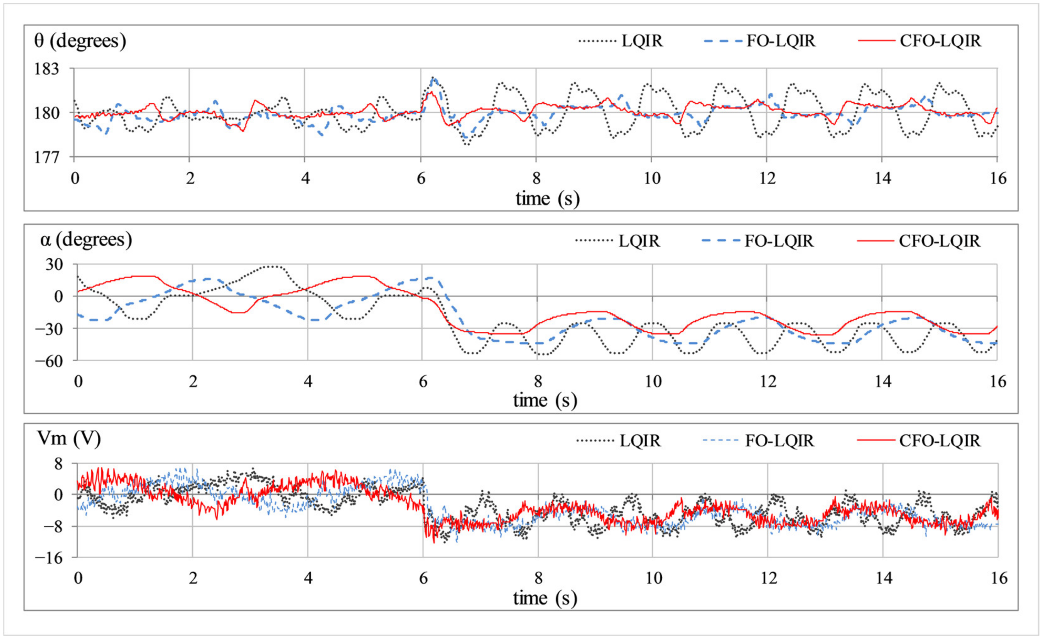
  • Step disturbance rejection: This experiment characterises the controller’s ability to reject sudden yet permanent load variations caused by constant exogenous forces. The pendulum is perturbed by artificially injecting a −5.0 V step signal in the control signal at t ≈ 6.0 s. The responses of α ( t ) , θ ( t ) , and V m ( t ) are shown in Figure 6.
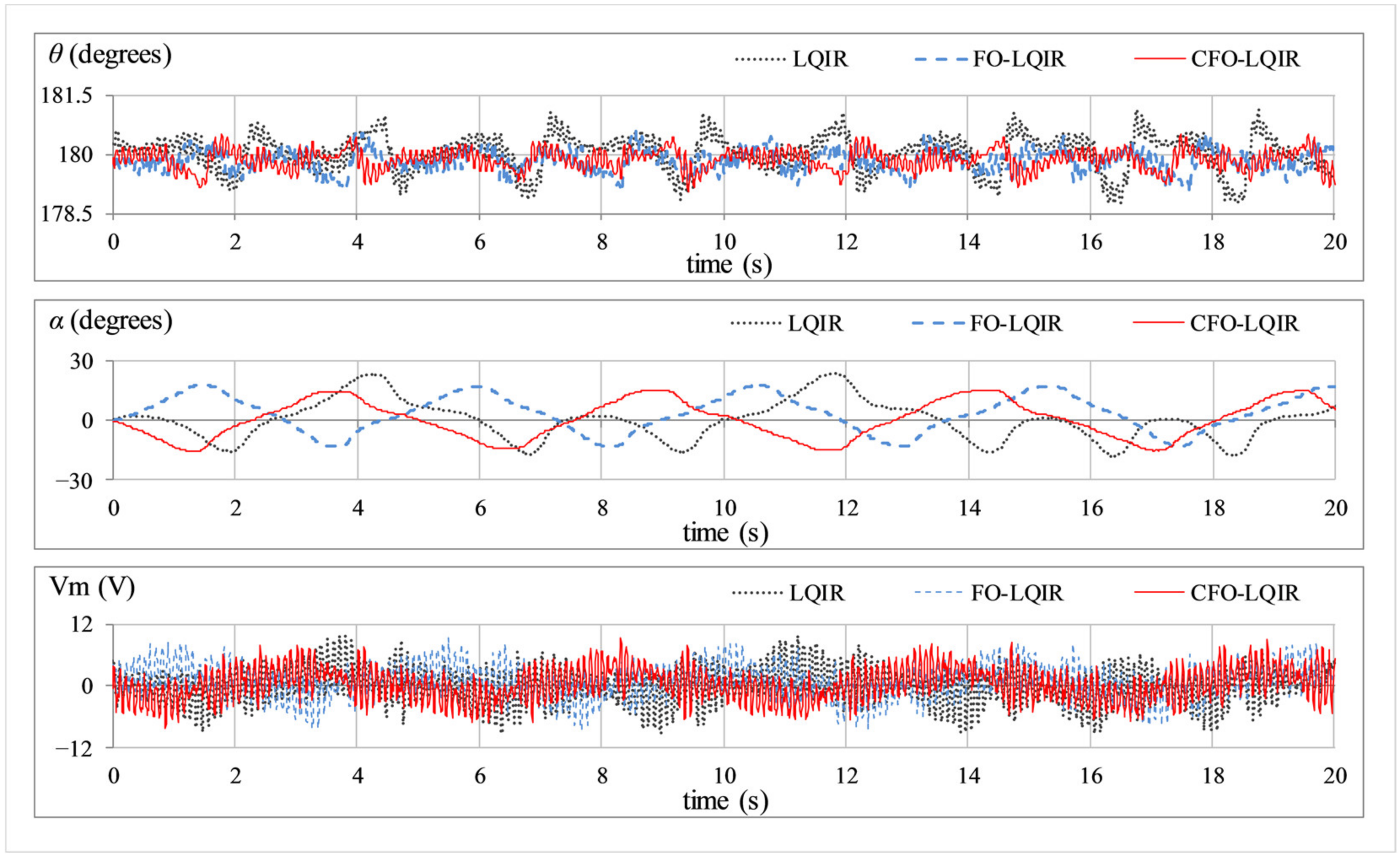
  • Sinusoidal noise attenuation: This experiment analyses the controller’s ability to attenuate the lumped disturbances caused by mechanical vibrations, measurement noise, and the chattering caused by the hysteresis in parasitic impedances. The test is performed by artificially injecting a sinusoidal signal of the form d ( t ) = sin ( 20   π t ) in the control signal. The responses of α ( t ) , θ ( t ) , and V m ( t ) are shown in Figure 7.
  • Modeling error compensation: The final experiment investigates the controller’s ability to compensate for the unprecedented modeling errors that are typically caused by inaccurate model identification or permanent model changes during the trials. The test is performed by attaching a 0.10 kg mass beneath the pendulum rod arm joint at t ≈ 6.0 s, as shown in Figure 4. This arrangement abruptly changes the actual system’s physical dynamics as compared to the reference model, which inevitably induces fluctuations in the state response(s). The responses of α ( t ) , θ ( t ) , and V m ( t ) are shown in Figure 8.

6.3. Discussion

The experimental outcomes are analysed as per the following Key Performance Indicators (KPIs).
  • ex_RMS: The root-mean-square value of error ( e α or e θ ), ( e x ( t ) ) 2 n .
  • ex_ITAE: The integral time-weighted absolute value of error ( e α or e θ ), t | e x ( t ) | d t .
  • ts,θ: The time taken by the pendulum’s apparatus rod to recover from a transient disturbance.
  • |Mp,x|: The magnitude of peak overshoot (or undershoot) contributed by the transient disturbances.
  • αoff: The offset in the arm’s position contributed by the step disturbance.
  • αp-p: The peak-to-peak amplitude of post-disturbance oscillations in the arm.
  • MSVm: The mean-square value of DC motor voltage.
  • Vp: The peak value of DC motor voltage under transient disturbances.
These standard KPIs are used in the scientific literature to correctly quantify the time domain performance of the SRIP system [47,48]. The quantitative analysis of the experimental results is presented in Table 2. The experimental results justify the enhanced robustness of CFO-LQIR in every experiment.
In experiment A (see Figure 4), the LQIR shows poor vertical position regulation accuracy of the rod and station keeping of the arm. The FO-LQIR exhibits mediocre improvement in the time domain behaviour. The CFO-LQIR manifests the best reference tracking accuracy while maintaining relatively economical control activity.
In experiment B (see Figure 5), the LQIR manifests large overshoots and a slow response speed. The FO-LQIR significantly improves the transit speed while suppressing the peak magnitude of the overshoots. The CFO-LQIR yields a relatively faster transient recovery speed while applying strong damping control effort to attenuate the overshoots. Furthermore, the CFO-LQIR also imposes minimal control input requirements upon the actuator under said disturbance conditions.
In experiment C (see Figure 6), the disturbance source renders highly disrupted control activity, which inevitably displaces the LQIR-driven pendulum arm with a large offset and induces large post-disturbance fluctuations in the arm as well as the apparatus rod. The FO-LQIR significantly improves the disturbance rejection capability, which leads to a smaller offset and fluctuations in the responses. The CFO-LQIR effectively minimises the offset in the arm’s position as well as the amplitude of post-disturbance fluctuations while expending less input energy and exhibiting smoother variations in the control profile.
In experiment D (see Figure 7), the LQIR and FO-LQIR both demonstrate weak immunity against the lumped disturbance along with large control input requirements. The CFO-LQIR effectively lowers the control input cost while effectively attenuating the chattering induced by the disturbance.
In experiment E (see Figure 8), the behaviour of the LQIR-driven system gets considerably degraded by the introduction of the parametric model variation. The FO-LQIR delivers reasonable modeling error compensation capability. The CFO-LQIR demonstrates the optimum model error rejection ability. The CFO-LQIR exhibits strong resilience against the modeling error and effectively damps the perturbations induced by it while curbing the overall control energy expenditure.
The superior disturbance rejection capability and response speed of the proposed CFO-LQIR are attributed to the enhanced flexibility in the controller design contributed by the complex orders associated with the integral/differential operators. These auxiliary terms increase the controller’s degrees of freedom to execute better realisation of the disturbances and thus perform better self-reasoning to flexibly manipulate the control input as the error conditions change. From an operational point of view, the cos ( . ) terms in the proposed control law (see (42)) act as gain modulators that depend on state error dynamics to regulate the differential and integral gains online. This arrangement not only increases the transient recovery speed and the damping against disturbances but also prevents the system from demanding large control input requirements. Although the tuning of a multitude of parameters poses a cumbersome task, the enhanced robustness and the flexibility to manipulate the control effort offered by the FO-LQIR outweighs this demerit.

6.4. A Special Comparison Case

In this article, a slightly modified variant of the proposed CFO-LQIR is also implemented and compared with the original CFO-LQIR procedure. The proposed modification is inculcated by changing the weight assignment in the cost function J c to tune the controller parameters. Thus, the controller parameters are re-calibrated offline by applying unequal weights to the constituents of the cost function, as shown below.
J c = 0 ( | e α ( t ) | 2 + 2 | e θ ( t ) | 2 + | u ( t ) | 2 ) d t
In this case, a larger weight is intentionally applied to the arm’s state error minimisation criteria in J c to observe its implications on the overall control behaviour of the proposed control law. The redesigned control law is referred to as the Modified CFO-LQIR (MCFO-LQIR). The tuning procedure prescribed in Section 3.2 is used. The coefficients of the Q and R matrices thus selected are given as q α = 39.4 , q θ = 55.2 , q α ˙ = 7.6 , q θ ˙ = 2.3 , and ρ = 1.02 . The re-calibrated matrices deliver the following state compensator gains: k α = 6.28 , k θ = 146.87 , k α ˙ = 4.72 , and k θ ˙ = 19.14 . The modified integral gains are k i α = 2.68 and k i θ = 6.95 × 10 6 . The real and imaginary parts of the new complex fractional orders chosen for the MCFO-LQIR law are β = 0.938 , γ = 0.894 , δ = 0.619 , μ = 0.315 , ρ = 1.861 , ε = 1.385 , σ = 0.077 , and φ = 0.086 . The position regulation and station-keeping capability of the SRIP system regulated by the MCFO-LQIR is compared with the CFO-LQIR under nominal conditions. The resulting responses of α ( t ) , θ ( t ) , and V m ( t ) are depicted in Figure 9.
The comparison reveals that the MCFO-LQIR scheme exhibits significant improvement in the arm’s position regulation accuracy as compared to the original CFO-LQIR. However, this improvement is achieved at the cost of highly discontinuous control activity and large control signal requirements, which inevitably inject chattering into the pendulum rod’s response, θ ( t ) . The results of this experiment are quantified in Table 3. This behaviour is caused by the application of unequal weights to the state error and control minimisation criteria in the cost function, which puts a relatively larger impact on the arm position regulation behaviour while affecting the overall control energy expenditure and the response of the apparatus rod.

7. Conclusions

This article systematically designs and implements an innovative complex-order controller to improve the robustness and disturbance rejection capability of an under-actuated and nonlinear SRIP system. For this purpose, a pre-calibrated set of complex-order integral and differential operators are augmented with a ubiquitous LQIR to improve the KPIs of the time domain performance. The proposed CFO-LQIR controller is compared against the integer-order LQIR and FO-LQIR. Especially, the introduction of the imaginary orders in the proposed CFO-LQIR increases the controller’s degree of freedom and improves its flexibility and adaptability to realise and reject the bounded exogenous disturbances. This augmentation equips the system to robustly handle nonlinear disturbances and parametric uncertainties. The aforementioned propositions are justified by analysing the experimental results collected from physical hardware. The proposed CFO-LQIR outperforms the other two controller variants in every test case by showing relatively faster transient recovery behaviour, lesser position regulation error, and stronger disturbance rejection. It remains optimum in every testing scenario by delivering rapid transits and strong damping against overshoots/undershoots as compared to its integer-order and fractional-order counterparts. Furthermore, the CFO-LQIR exhibits economical control energy expenditure and minimal position regulation error in the rod as compared to those of the MCFO-LQIR variant. In the future, the efficacies of using complex-order controllers with adaptively self-adjusting real and imaginary orders for under-actuated systems can be investigated. Furthermore, the mentioned control scheme has the potential to be extended and applied to other nonlinear dynamical and cyber-physical systems.

Author Contributions

Conceptualization, O.S.; methodology, O.S. and F.A.; software, O.S. and F.A..; validation, J.I.; formal analysis, O.S; investigation, O.S. and F.A.; resources, J.I.; data curation, F.A.; writing—original draft preparation, O.S.; writing—review and editing, J.I.; visualization, J.I.; supervision, J.I.; project administration, J.I.; All authors have read and agreed to the published version of the manuscript.

Funding

This research received no external funding.

Data Availability Statement

The authors declare that the data analysed during this study to support the findings will be made available on reasonable request.

Conflicts of Interest

The authors declare no conflict of interest.

References

  1. Li, Z.; Yang, C.; Fan, L. Advanced Control of Wheeled Inverted Pendulum Systems; Springer: London, UK, 2013. [Google Scholar]
  2. Johnson, T.; Zhou, S.; Cheah, W.; Mansell, W.; Young, R.; Watson, S. Implementation of a Perceptual Controller for an Inverted Pendulum Robot. J. Intell. Robot. Syst. 2020, 99, 683–692. [Google Scholar] [CrossRef]
  3. Krafes, S.; Chalh, Z.; Saka, A. A Review on the Control of Second Order Underactuated Mechanical Systems. Complexity 2018, 2018, 9573514. [Google Scholar] [CrossRef]
  4. Ilyas, M.; Khaqan, A.; Iqbal, J.; Riaz, R.A. Regulation of hypnosis in Propofol anesthesia administration based on non-linear control strategy. Braz. J. Anesthesiol. 2017, 67, 122–130. [Google Scholar] [CrossRef] [PubMed]
  5. Koryakovskiy, I.; Kudruss, M.; Babuška, R.; Caarls, W.; Vallery, H. Benchmarking model-free and model-based optimal control. Robot. Auton Syst 2017, 92, 81–90. [Google Scholar] [CrossRef]
  6. Sirisha, V.; Junghare, A.S. A Comparative study of controllers for stabilizing a Rotary Inverted Pendulum. Int. J. Chaos Control Model. Simul. 2014, 3, 1–13. [Google Scholar] [CrossRef]
  7. Huang, A.-C.; Kai, C.-Y.; Chen, Y.-F. Adaptive Control of Underactuated Mechanical Systems; World Scientific: Singapore, 2015. [Google Scholar]
  8. Gritli, H.; Belghit, S. Robust feedback control of the underactuated Inertia Wheel Inverted Pendulum under parametric uncertainties and subject to external disturbances: LMI formulation. J. Franklin Inst. 2018, 355, 9150–9191. [Google Scholar] [CrossRef]
  9. Lee, H.; Gil, J.; You, S.; Gui, Y.; Kim, W. Arm Angle Tracking Control with Pole Balancing Using Equivalent Input Disturbance Rejection for a Rotational Inverted Pendulum. Mathematics 2021, 9, 2745. [Google Scholar] [CrossRef]
  10. Rojsiraphisal, T.; Mobayen, S.; Asad, J.H.; Vu, M.T.; Chang, A.; Puangmalai, J. Fast Terminal Sliding Control of Underactuated Robotic Systems Based on Disturbance Observer with Experimental Validation. Mathematics 2021, 9, 1935. [Google Scholar] [CrossRef]
  11. Iqbal, J. Modern control laws for an articulated robotic arm: Modelling and simulation. Eng. Technol. Appl. Sci. Res. 2019, 9, 4057–4061. [Google Scholar] [CrossRef]
  12. Wang, J.J. Simulation studies of inverted pendulum based on PID controllers. Simul. Model. Pract. Theory 2011, 19, 440–449. [Google Scholar] [CrossRef]
  13. Iqbal, J.; Heikkila, S.; Halme, A. Tether tracking and control of ROSA robotic rover. In Proceedings of the 10th IEEE International Conference on Control, Automation, Robotics and Vision, Vietnam, Hanoi, Vietnam, 17–20 December 2008; pp. 689–693. [Google Scholar]
  14. Khan, O.; Pervaiz, M.; Ahmad, E.; Iqbal, J. On the derivation of novel model and sophisticated control of flexible joint manipulator. Revue Roumaine des Sciences Techniques-Serie Electrotechnique et Energetique 2017, 62, 103–108. [Google Scholar]
  15. Balamurugan, S.; Venkatesh, P.; Varatharajan, M. Fuzzy sliding-mode control with low pass filter to reduce chattering effect: An experimental validation on Quanser SRIP. Sadhana 2017, 42, 1693–1703. [Google Scholar] [CrossRef]
  16. Anjum, M.; Khan, Q.; Ullah, S.; Hafeez, G.; Fida, A.; Iqbal, J.; Albogamy, F.R. Maximum power extraction from a standalone photo voltaic system via neuro-adaptive arbitrary order sliding mode control strategy with high gain differentiation. Appl. Sci. 2022, 12, 2773. [Google Scholar] [CrossRef]
  17. Bhatti, O.S.; Tariq, O.B.; Manzar, A.; Khan, O.A. Adaptive intelligent cascade control of a ball-riding robot for optimal balancing and station-keeping. Adv. Robot. 2018, 32, 63–76. [Google Scholar] [CrossRef]
  18. Wang, X.; Abtahi, S.M.; Chahari, M.; Zhao, T. An Adaptive Neuro-Fuzzy Model for Attitude Estimation and Control of a 3 DOF System. Mathematics 2022, 10, 976. [Google Scholar] [CrossRef]
  19. Sukontanakarn, V.; Parnichkun, M. Real-Time Optimal Control for Rotary Inverted Pendulum. Am. J. Appl. Sci. 2009, 6, 1106–1115. [Google Scholar]
  20. Prasad, L.B.; Tyagi, B.; Gupta, H.A. Optimal Control of Nonlinear Inverted Pendulum System Using PID Controller and LQR: Performance Analysis Without and With Disturbance Input. Int. J. Autom. Comput. 2014, 11, 661–670. [Google Scholar] [CrossRef]
  21. Faisal, R.F.; Abdulwahhab, O.W. Design of an Adaptive Linear Quadratic Regulator for a Twin Rotor Aerodynamic System. J. Control Autom. Electr. Syst. 2021, 32, 404–415. [Google Scholar] [CrossRef]
  22. Dwivedi, P.; Pandey, S.; Junghare, A.S. Stabilization of Unstable Equilibrium Point of Rotary Inverted Pendulum using Fractional Controller. J. Frankl. Inst. 2017, 354, 7732–7766. [Google Scholar] [CrossRef]
  23. Li, Z.; Liu, L.; Dehgan, S.; Chen, Y.Q.; Xue, D. A review and evaluation of numerical tools for fractional calculus and fractional order controls. Int. J. Control 2017, 90, 1165–1181. [Google Scholar] [CrossRef]
  24. Kumar, N.; Alotaibi, M.A.; Singh, A.; Malik, H.; Nassar, M.E. Application of Fractional Order-PID Control Scheme in Automatic Generation Control of a Deregulated Power System in the Presence of SMES Unit. Mathematics 2022, 10, 521. [Google Scholar] [CrossRef]
  25. Saleem, O.; Mahmood-ul-Hasan, K. Robust stabilisation of rotary inverted pendulum using intelligently optimised nonlinear self-adaptive dual fractional order PD controllers. Int. J. Syst. Sci. 2019, 50, 1399–1414. [Google Scholar] [CrossRef]
  26. Dwivedi, P.; Pandey, S.; Junghare, A.S. Robust and novel two degree of freedom fractional controller based on two-loop topology for inverted pendulum. ISA Trans 2018, 75, 189–206. [Google Scholar] [CrossRef] [PubMed]
  27. Abdulwahhab, O.W.; Abbas, N.H. A New Method to Tune a Fractional-Order PID Controller for a Twin Rotor Aerodynamic System. Arab. J. Sci. Eng. 2017, 42, 5179–5189. [Google Scholar] [CrossRef]
  28. Shahiri, M.; Ranjbar, A.; Karami, M.; Ghaderi, R. Robust control of nonlinear PEMFC against uncertainty using fractional complex order control. Nonlinear Dyn. 2015, 80, 1785–1800. [Google Scholar] [CrossRef]
  29. Guefrachi, A.; Najar, A.; Amairi, M.; Aoun, M. Tuning of fractional complex order PID controller. IFAC−PapersOnLine 2017, 50, 14563–14568. [Google Scholar]
  30. Abdulwahhab, O.W. Design of a complex fractional order PID controller for a first order plus time delay system. ISA Trans 2020, 99, 154–158. [Google Scholar] [CrossRef]
  31. Shah, P.; Sekhar, R.; Iswanto, I.; Shah, M. Complex Order PIa+jbDc+jd Controller Design for a Fractional Order DC Motor System. Adv. Sci. Technol. Eng. Syst. J. 2021, 6, 541–551. [Google Scholar] [CrossRef]
  32. Tare, A.; Jacob, J.; Vyawahare, V.; Pande, V. Design of novel optimal complex-order controllers for systems with fractional-order dynamics. Int. J. Dyn. Control 2019, 7, 355–367. [Google Scholar] [CrossRef]
  33. Irfan, A.; Mehmood, A.; Razzaq, M.T.; Iqbal, J. Advanced sliding mode control techniques for inverted pendulum: Modelling and simulation. Eng. Sci. Technol. Int. J. 2018, 21, 753–759. [Google Scholar] [CrossRef]
  34. Jian, Z.; Yongpeng, Z. Optimal Linear Modeling and its Applications on Swing-up and Stabilization Control for Rotary Inverted Pendulum. In Proceedings of the 30th Chinese Control Conference, Yantai, China, 22–24 July 2011; pp. 493–500. [Google Scholar]
  35. Astom, K.J.; Apkarian, J.; Karam, P.; Levis, M.; Falcon, J. Student Workbook: QNET Rotary Inverted Pendulum Trainer for NI ELVIS; Quanser Inc.: Markham, ON, Canada, 2011. [Google Scholar]
  36. Lewis, F.L.; Vrabie, D.; Syrmos, V.L. Optimal Control; John Wiley and Sons: Hoboken, NJ, USA, 2012. [Google Scholar]
  37. Valencia-Rivera, G.H.; Merchan-Villalba, L.R.; Tapia-Tinoco, G.; Lozano-Garcia, J.M.; Ibarra-Manzano, M.A.; Avina-Cervantes, J.G. Hybrid LQR-PI Control for Microgrids under Unbalanced Linear and Nonlinear Loads. Mathematics 2020, 8, 1096. [Google Scholar] [CrossRef]
  38. Saleem, O.; Rizwan, M.; Mahmood-ul-Hasan, K. Self-tuning state-feedback control of a rotary pendulum system using adjustable degree-of-stability design. Automatika 2021, 62, 84–97. [Google Scholar] [CrossRef]
  39. Das, S.; Pan, I.; Halder, K.; Das, S.; Gupta, A. Optimum weight selection based LQR formulation for the design of fractional order PIλDμ controllers to handle a class of fractional order systems. In Proceedings of the 2013 International Conference on Computer Communication and Informatics, Coimbatore, India, 4–6 January 2013; pp. 1–6. [Google Scholar]
  40. Micev, M.; Ćalasan, M.; Oliva, D. Fractional Order PID Controller Design for an AVR System Using Chaotic Yellow Saddle Goatfish Algorithm. Mathematics 2020, 8, 1182. [Google Scholar] [CrossRef]
  41. Mishra, S.K.; Chandra, D. Stabilization and Tracking Control of Inverted Pendulum Using Fractional Order PID Controllers. J. Eng. 2014, 2014, 752918. [Google Scholar] [CrossRef]
  42. Saleem, O.; Awan, F.G.; Mahmood-ul-Hasan, K.; Ahmad, M. Self-adaptive fractional-order LQ-PID voltage controller for robust disturbance compensation in DC-DC buck converters. Int. J. Numer. Model. 2020, 33, e2718. [Google Scholar] [CrossRef]
  43. Monje, C.; Chen, Y.; Vinagre, B.; Xue, D.; Feliu, V. Fractional Order Systems and Control—Fundamentals and Applications; Springer: London, UK, 2010. [Google Scholar]
  44. Shahiri, M.; Ranjbar, A.; Karami, M.R.; Ghaderi, R. New tuning design schemes of fractional complex-order PI controller. Nonlinear Dyn. 2016, 84, 1813–1835. [Google Scholar] [CrossRef]
  45. Sekhar, R.; Singh, T.P.; Shah, P. Complex Order PIα+jβDγ+jθ Design for Surface Roughness Control in Machining CNT Al-Mg Hybrid Composites. Adv. Sci. Technol. Eng. Syst. J. 2020, 5, 299–306. [Google Scholar] [CrossRef]
  46. Astrom, K.J.; Apkarian, J.; Karam, P.; Levis, M.; Falcon, J. Instructor Workbook: QNET Rotary Invrted Pendulum Trainer for NI ELVIS; Quanser: Markham, ON, Canada, 2011; pp. 24–26. [Google Scholar]
  47. Saleem, O.; Mahmood-ul-Hasan, K.; Rizwan, M. An Experimental Comparison of Different Hierarchical Self-Tuning Regulatory Control Procedures for Under-Actuated Mechatronic Systems. PLoS ONE 2021, 16, e0256750. [Google Scholar] [CrossRef]
  48. Hfaiedh, A.; Chemori, A.; Abdelkrim, A. Stabilization of the Inertia Wheel Inverted Pendulum by Advanced IDA-PBC Based Controllers: Comparative Study and Real-Time Experiments. In Proceedings of the SSD 2022 17th International Multi-Conference on Systems, Signals & Devices, Monastir, Tunisia, 20–23 July 2020; pp. 753–760. [Google Scholar]
Figure 1. Simplified schematic of the SRIP system.
Mathematics 11 00913 g001
Figure 2. Block diagram of the proposed CFO-LQIR law.
Mathematics 11 00913 g002
Figure 3. QNET rotary pendulum setup.
Mathematics 11 00913 g003
Figure 4. SRIP’s response under normal conditions.
Mathematics 11 00913 g004
Figure 5. SRIP’s response under impulsive disturbances.
Mathematics 11 00913 g005
Figure 6. SRIP’s response under step disturbance.
Mathematics 11 00913 g006
Figure 7. SRIP’s response under sinusoidal disturbance.
Mathematics 11 00913 g007
Figure 8. SRIP’s response under model variation.
Mathematics 11 00913 g008
Figure 9. Response of CFO-LQIR versus MCFO-LQIR under nominal conditions.
Mathematics 11 00913 g009
Table 1. Model parameters of QNET rotary pendulum.
ParametersDescriptionValueUnits
MpMass of pendulum0.027kg
lpPendulum center of mass0.153m
LpLength of pendulum rod0.191M
rLength of horizontal arm0.083M
MarmMass of arm0.028Kg
gGravitational acceleration9.810m/s2
JeMoment about motor shaft1.23 × 10−4kgm2
JpMoment about pendulum1.10 × 10−4kgm2
RmMotor armature resistance3.30Ω
LmMotor armature inductance47.0mH
KtMotor torque constant0.028Nm
KmBack e.m.f. constant0.028V/(rad/s)
TmMaximum torque0.14Nm
Table 2. Summary of experimental results.
ExperimentKPIControl Scheme
SymbolUnitLQIRFO-LQIRCFO-LQIR
Aeθ_RMSdegrees0.530.430.36
eθ_ITAEs.degrees7.846.155.35
eα_RMSdegrees15.6911.8510.08
eα_ITAEs.degrees263.50196.18167.61
MSVmV28.478.207.18
Beθ_RMSdegrees0.710.640.47
eθ_ITAEs.degrees9.649.306.44
|Mp,θ|degrees2.772.482.23
ts,θs0.720.580.51
eα_RMSdegrees11.5110.349.68
eα_ITAEs.degrees189.14168.30161.69
MSVmV29.618.226.39
VpV−9.85−9.63−8.47
Ceθ_RMSdegrees1.120.560.42
eθ_ITAEs.degrees18.278.327.52
eα_RMSdegrees32.4728.1022.06
eα_ITAEs.degrees524.41458.96380.65
αoffdegrees−38.46−33.02−23.72
αp-pdegrees−28.74−30.75−21.61
MSVmV227.9328.6825.35
VpV−11.73−10.52−10.34
Deθ_RMSdegrees0.460.320.29
eθ_ITAEs.degrees7.245.134.50
eα_RMSdegrees10.149.859.53
eα_ITAEs.degrees160.08165.78160.63
MSVmV212.6211.7310.50
Eeθ_RMSdegrees1.060.900.78
eθ_ITAEs.degrees15.8312.8211.88
eα_RMSdegrees16.0112.9711.78
eα_ITAEs.degrees281.17223.89201.48
MSVmV211.4410.639.48
Table 3. Summary of experiment to compare MCFO-LQIR with CFO-LQIR.
KPIControl Scheme
SymbolUnitCFO-LQIRMCFO-LQIR
eθ_RMSdegrees0.360.40
eθ_ITAEs.degrees5.356.32
eα_RMSdegrees10.087.34
eα_ITAEs.degrees167.61121.65
MSVmV27.1813.50
VpV7.05−14.61
Disclaimer/Publisher’s Note: The statements, opinions and data contained in all publications are solely those of the individual author(s) and contributor(s) and not of MDPI and/or the editor(s). MDPI and/or the editor(s) disclaim responsibility for any injury to people or property resulting from any ideas, methods, instructions or products referred to in the content.

