1. Introduction
In recent years, multi-degree-of-freedom (DOF) industrial robots have been widely used in assembly, handling and other industries [
1,
2,
3]. They can replace repetitive machine-type manipulation, and they are servo devices that rely on their own power and control to achieve multiple functions. With the rapid development of modern manufacturing, requirements for the control accuracy, running speed and system stability of industrial robots are increasing [
4].
A robot system includes a driving device, a transmission device and the robot body. Driving devices mostly adopt PMSM [
5], due to PMSM having the characteristics of high accuracy, wide speed range, low speed and fast dynamic response. Transmission devices widely adopt harmonic drive. PMSM converts electromagnetic torque into joint torque using harmonic drive, which can drive the robot joints to complete specified motions and functions.
The transmission mechanism in harmonic drive is rolling transmission, and friction is represented by rolling friction. As a dynamic friction model, the LuGre friction model explains the relationship between nonlinear force, Coulomb friction, viscous friction and the Stribeck effect. It describes friction force as a function of relative velocity between the contact surfaces [
6,
7,
8]. The harmonic drive is divided into the motor side and the joint side in this paper. Dynamic equations based on the LuGre friction model are established in order to improve the generalized mathematical model of the robot joint servo system.
The process of researching PMSM-driven robot joints is currently accelerating, and researchers have made great progress in this area of science and technology innovation. However, there are still many problems to be solved related to the servo control of robot joint systems. In the actual industrial production, creating robot joints that have both superior response speed and control accuracy, and remain stable during the whole process of operation, has become a key technology problem in the research field of PMSM-driven robot joint servo control system [
9,
10].
Domestic and foreign researchers have carried out a large amount of research work with the aim of improving performance of control and optimization of PMSM-driven robot joints. Depending on the controller used, the design of servo control of robot joints can be divided into two types: signal control and energy control. From the point of view of signal control [
11,
12], the servo control system of a robot joint is considered to be a signal conversion device that converts the input position signal into the output position signal. Although a signal controller can achieve the control requirement of fast dynamic response, the electrical characteristics of PMSM and the friction characteristics of robot joints are not considered. Due to high energy consumption and loss of friction, the optimization of energy loss in the steady state cannot be achieved. Therefore, the steady-state error of the system is large, and vibration occurs during the operation of a robot joint when the signal controller is used alone. In contrast, from the point of view of energy control [
13,
14], the servo control system of a robot joint is considered an energy conversion device. It converts the given input energy into the actual output energy. The energy controller can cause the system to track accurately in the steady state and stabilise the joint during operation, but the dynamic response speed is very slow.
Based on the view of signal control, many control strategies have been proposed. These include backstepping control [
15], sliding mode control [
16], fuzzy control [
17], robust control [
18,
19], adaptive control [
20], etc.
The backstepping control (BC) algorithm is simple and makes the design process of a controller systematized and structured. BC is often combined with intelligent methods and other nonlinear methods in the position control of robot joint servo systems [
21,
22].
Sliding mode control (SMC) is extensively applied in nonlinear systems, due to its strong robustness against external disturbances and parameter perturbations. Traditional SMC has many obstacles in practical application; for instance, it cannot make systems converge in a limited time, and shows a obvious chattering phenomenon during the operation of the robot joints [
23,
24]. However, SMC has the merit of quick regulation, which can result in nonlinear systems having faster dynamic response speeds than with other control methods [
25].
An accurate mathematical model cannot be established for the robot joint servo system, so fuzzy control [
26] has been proposed. However, the steady-state error of the systems in this case is large and the control effect is unsatisfactory.
As a kind of robust control,
shows strong robustness in the field of controlling robot joints. In [
27], a controller for robot joints is designed using a
frame. It can precisely follow target signals and has good robustness. However, the design scheme of
is complicated and difficult to implement. The above research algorithms all stem from the viewpoint of signal control. Although they promote the response speed of robot joint servo systems, their steady-state error rates are large.
At present, scientific researchers are concerned with research into algorithms approaching the problem from the viewpoint of energy control. Ortega et al. proposed the port-controlled Hamiltonian (PCH) [
28,
29,
30,
31] control method, which uses a dissipative PCH model to represent the dynamic system. It can diminish the steady-state error of a robot joint’s servo system during operation. Nevertheless, the rapidity of this system is poor, and its dynamic properties are difficult to guarantee.
To sum up, both single signal control methods and energy control methods have their own weaknesses. In order to develop a system with both superior rapidity and accuracy at the same time, the strategy of optimized cooperative control is put forward in this paper. The strategy of optimized cooperative control adopts a optimized cooperative control coefficient based on the position error of robot joints, so that the system can smoothly switch between the signal controller and the energy controller. The signal controller occupies centre stage and guarantees the rapidity of system when the error of a joint is large. When the error is small, control switches from the signal controller to the energy controller. At this time, the energy controller occupies centre stage and guarantees the accuracy of the system. In this way, the robot joint benefits from the advantages of the signal controller and the energy controller. The system has short response time and low tracking error when robot joints are tracking target signals. Generalized mathematical models of the robot joint servo system are expressed by combining the robot body’s dynamics equation, motor characteristics and joint friction. The EPCH energy controller and ABSM signal controller are both designed using the generalized mathematical model. A Gaussian function is used as the optimized cooperative control coefficient, and the strategy of cooperative optimization control of EPCH and ABSM is designed. Finally, simulation results show that this strategy results in a robot system that has both fast response speed and high tracking accuracy.
The structure of this article is as follows. In
Section 2, the kinetic equation of a multi-joint industrial robot is given. In
Section 3, the EPCH energy controller, ABSM signal controller and the strategy of optimized cooperative control are designed. In
Section 4, we testify to the availability of optimized cooperative control through simulation results. The conclusion is given in
Section 5.
2. Mathematical Model of Multi-Joint Industrial Robot
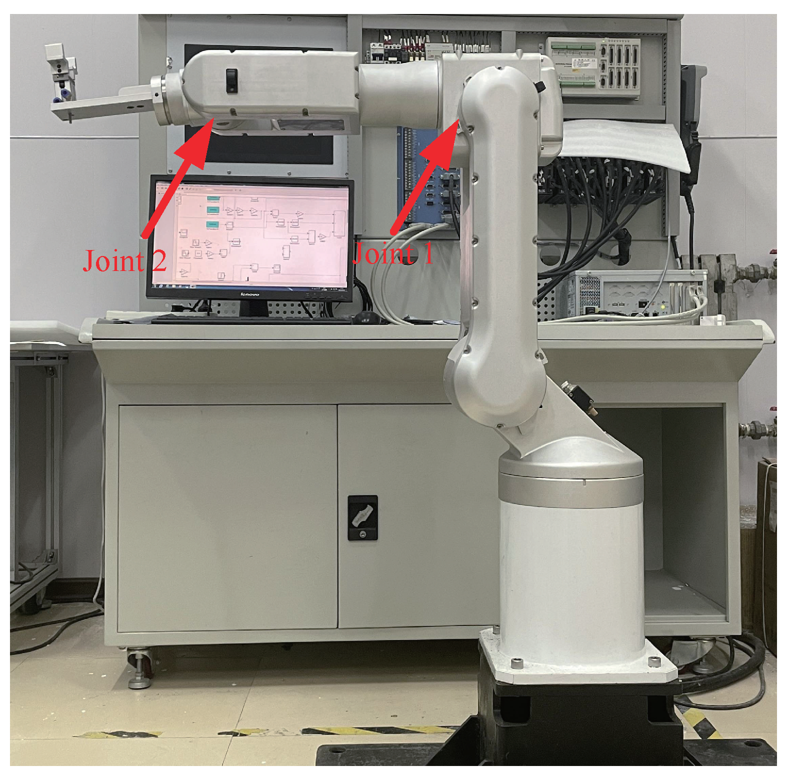
This paper takes the servo system of a 2-DOF robot as the object of study. The multi-joint industrial robot servo system is displayed in
Figure 1. It includes three parts: PMSM, harmonic drive and robot body. The Lagrange’s equation of the robot body is described as [
32]
where
,
and
denote the position, velocity and acceleration, respectively.
is the positive and definite inertia matrix.
includes the Coriolis and centripetal forces.
is the vector of gravity terms.
is the moment of the robot joint.
denotes the Coulomb friction coefficient matrix of robot joints.
is a vector of external force.
is the Jacobian matrix.
The parameters of robot body is presented in the
Appendix A.
To establish the mathematical model of PMSM, the following conditions are described:
- 1.
The influence of the core saturation phenomenon is not considered.
- 2.
The damping effects of the permanent magnet and rotor are ignored.
- 3.
The material of the permanent magnet is considered to be insulated.
- 4.
It is determined that the magnetic circuit is linear and satisfies the superposition theorem.
In a synchronously rotating
d-q reference frame, the model of the
i-th (
i = 1, 2) PMSM with implicit pole type (
) can be described as [
33]
where
is the electromagnetic torque of PMSM.
is the torque of the robot joint.
and
denote the stator voltages of the
d-axis and
q-axis, respectively.
and
denote the stator inductances of the
d-axis and
q-axis, respectively.
and
denote the stator currents of the
d-axis and
q-axis, respectively.
is the stator resistance per phase.
is the rotor flux linking of the stator.
is the number of pole pairs in PMSM.
is the angle.
is the moment of inertia in PMSM.
is the friction coefficient of PMSM.
is the angular velocity.
We can learn from
and
that
The i-th harmonic drive is decomposed into a dynamic model consisting of the motor side and joint side. The motor side is connected to the PMSM, and the joint side is connected to the robot joint.
The model of the motor side is
The model of the joint side is
where
is the load moment of the motor side.
is the friction torque of the motor side.
is the friction torque of the joint side.
is the moment of inertia of the motor side.
is the moment of inertia of the joint side.
is the angular acceleration of the motor shaft.
is the angular acceleration of the robot joint.
is the reduction ratio of the harmonic drive, and
.
The LuGre model expression of
is
where
and
denote the average bristle deformation amount and deformation rate of the high-speed axis, respectively.
,
,
,
, respectively, denote the Coulomb friction, Stribeck friction, Stribeck velocity and static friction functions of high-speed shafts.
,
and
denote the bristle stiffness, bristle damping and viscous friction of the motor side, respectively.
The LuGre model expression of
is
where
and
denote the average bristle deformation amount and deformation rate of the low-speed axis, respectively.
,
,
,
, respectively, denote the Coulomb friction, Stribeck friction, Stribeck velocity and static friction functions of low-speed shafts.
,
and
denote the bristle stiffness, bristle damping and viscous friction of the joint side, respectively.
is the angular velocity of the robot joint.
Because the material, quality and lubrication conditions of the motor side and the joint side of the harmonic drive are almost all the same, the parameters of the LuGre model take the same values.
From Equations (
1)–(
9), the generalized model of the robot joint servo system is deduced as
where
The dynamic equation (Equation (
10)) of the robot system satisfies the following properties [
34].
- (1)
is the positive definite symmetric matrix, and an inverse matrix
exists.
and
, as functions of
, are uniformly bounded. Namely, the existence of
and
makes the following equation hold:
- (2)
is the skew symmetric matrix. Namely,
can satisfy the following equation:
3. Design of Optimized Cooperative Control
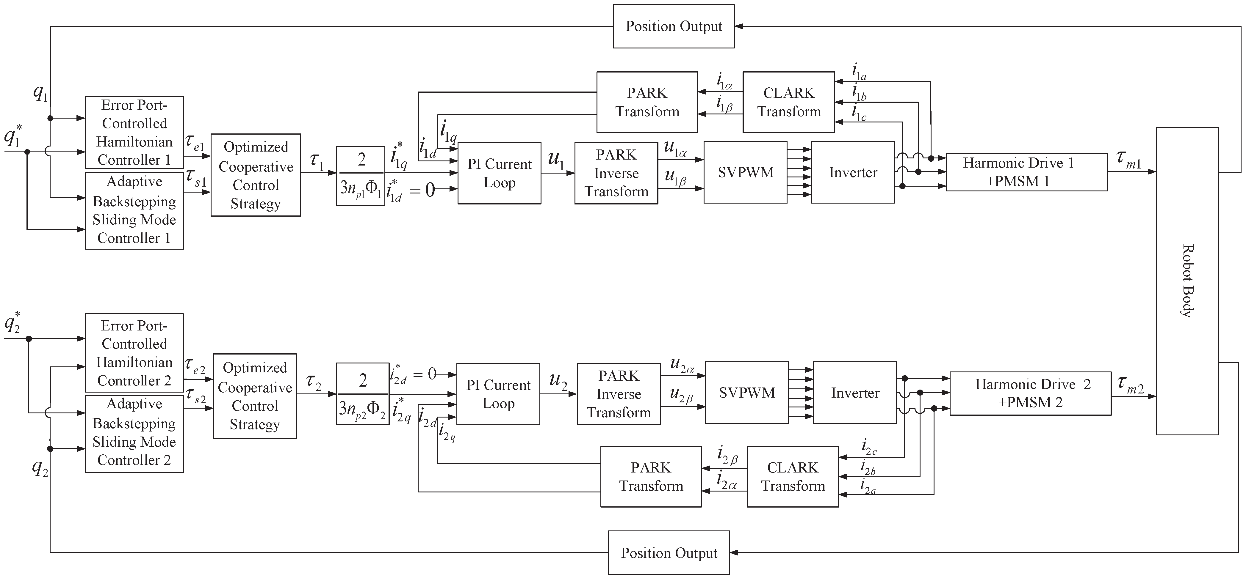
The control graph of the optimized cooperative control of a 2-DOF robot servo system is displayed in
Figure 2.
and
are the practical positions and expected positions of the robot joint, respectively.
are the output torque of the EPCH energy controller,
are the output torque of the ABSM signal controller,
is the output torque after the application of optimized cooperative control,
are the electromagnetic torque of PMSM, and
are the output voltage of PMSM. The inverter is a triphase inverter. Space Vector Pulse Width Modulation (SVPWM) is the pulse width modulation technology, which generates a pulse width modulation wave by switching mode. It considers the inverter system and PMSM as a whole, and the model is relatively simple.
The PI current loop is designed as follows:
where
,
are, respectively, the scale coefficient and integral coefficient of the PI current loop, which includes the adjustment of parameters
,
and
.
Because the current loop adopts PI control, the PMSM parameters , and do not need to be adjusted, and only the parameters and of the PI current loop need to be adjusted.
3.1. Design of EPCH Energy Controller
For a nonlinear system, the PCH model of the EPCH energy controller with energy dissipation can be calculated as [
35,
36,
37,
38]
where
,
, and
are the state vector, control vector, and output vector.
is the interconnection matrix,
, which expresses the interconnection structure.
is the damping matrix,
, which shows the resistive structure on the port.
reflects the port’s characteristics.
is the Hamiltonian function, which signifies the total energy stored by the system.
The state vector, control vector and position error of the robot joints are defined, respectively, as
where
denotes the generalized inertia matrix of the system, and
denotes the expected value of the robot joint’s motion trajectory.
The Hamiltonian function
of robot joints is defined as
where
is the potential energy of the robot joints.
Taking the partial differentiation of Equation (
23), we can get
Using Equations (17) and (24), we have
Then, combining Equations (19), (24) and (25), the PCH model of a 2-DOF robot is expressed as
where
Introducing state error into the PCH model can further improve the tracking accuracy of the system. The following is the design process of the EPCH controller.
The state error of the robot joints is
where
is the expected state matrix.
The expected Hamiltonian function, including the kinetic energy and potential energy of the robot joint, is chosen as
where
denotes the moment of inertia, and
indicates the kinetic energy of the robot joints.
denotes the proportional gain and
indicates the potential energy of robot joints.
Calculating the derivation of Equation (
31), we have
when the system is in equilibrium, that is,
, the internal storage energy of the system is the smallest. At this time, the form of the EPCH is expressed as
where the expected interconnection matrix
and expected damping matrix
are chosen as
The gain of damping matrix .
From Equations (26), (30) and (33), we can get
Using Equation (
36), we can obtain the control law
where
,
.
The desired Hamiltonian function (31) is the Lyapunov function, so the Lyapunov function
is
From the derivation of Equation (
38), we can obtain
Substituting Equations (10) and (37) into Equation (
39), we can get
is the largest invariant set of . Therefore, according to the Lasalle invariant set principle, the closed-loop control system of the robot is asymptotically stable at the equilibrium point.
3.2. Design of ABSM Signal Controller
The EPCH energy controller has the advantages of high precision and strong stability. However, its dynamic properties are not ideal when it is used alone. Therefore, the ABSM signal controller is proposed to compensate for the dynamic properties.
Before the construction of the ABSM signal controller, it is required to improve the dynamic equation of the robot joint system. We need to replace the friction moment term
with the uncertainty term
, and construct an adaptive law to estimate the uncertainty term
in real time, that is, making
. Then, Equation (
10) is represented as
where
only includes friction interference caused by PMSM, harmonic drive and the robot body, and any other external interference is not considered.
The design of the ABSM signal controller is as follows. Equation (
41) is converted to a state space expression:
Step 1: The position error of the robot joints is defined as
where
denotes the desired position of the robot joint.
Taking the derivative of Equation (
43), we get
We take the virtual control quantity
and define
The Lyapunov function of the subsystem of Step 1 is selected as
We conduct the derivative of Equation (
46) and use Equation (
45) to obtain
In Equation (
47), if
, then
. Therefore, the next step of the design is needed.
Step 2: Taking the derivative of Equation (
44) and using Equation (
42), we get
The sliding surface of a traditional SMC is selected as
where
denotes the positive constant value matrix.
By calculating the derivative of Equation (
49) and using Equation (
42), we have
We define the Lyapunov function of subsystem of Step 2 as
We conduct the derivative of Equation (
51) and combine Equations (47) and (50) to obtain
The estimation error is defined as
where
is the estimated value of the uncertainty term
, and
.
Based on Equation (
51), the Lyapunov function is defined at this time as
where
is the normal number matrix.
By taking the derivative of Equation (
54), and combining Equation (
52) with Equation (
53), we can get
In order to simplify Equation (
55) and further prove
, the control torque of the robot joint is selected
where
is the symmetric and positive constant value matrix, and
is a normal number.
The adaptive law can be taken as
The Lyapunov function of the whole robot system is defined as
By taking the derivative of Equation (
58), and substituting Equations (56) and (57) into Equation (
55), we get
We take
, and take the appropriate value to turn
into the positive definite matrix. We have
, and get
With the design of the above controller, the sliding surface can ultimately be bounded as stable, and the robot joints can move according to the desired trajectory.
3.3. Strategy of Optimized Cooperative Control
3.3.1. Design of Optimized Cooperative Controller
The ABSM signal controller contributes rapid response speed and outstanding dynamic performance to the system; the EPCH energy controller generates high tracking precision and impressive steady-state behavior. The strategy of optimized cooperative control is designed to combine the advantages of these two controllers. Additionally, the coefficient matrix of optimized cooperative control is introduced in order to make the control vector change continuously and smoothly in the optimized cooperative control procedure.
The design of the optimized cooperative controller is calculated as
where
denotes the input torque of a joint after optimized cooperative control,
is the coefficient matrix of optimized cooperative control based on the position error of the robot joint, and
.
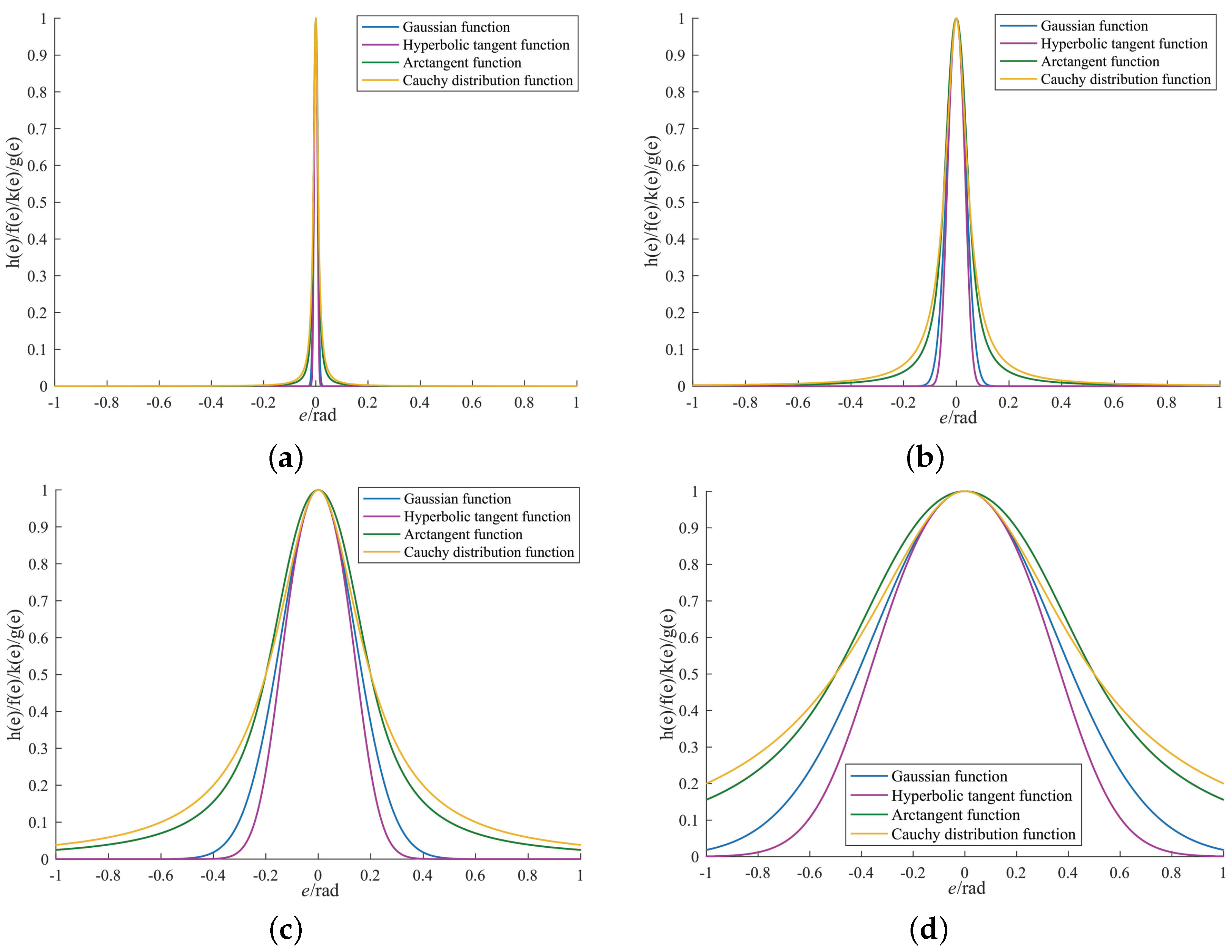
There are many kinds of mathematical function that can be used as cooperative control coefficients, and different cooperative control coefficients have different effects on the cooperative control of the system. In order to study which coefficient has the best effect on the cooperative control of the system, four kinds of cooperative control coefficient, namely a Gaussian function, hyperbolic tangent function, arctangent function, and Cauchy distribution function, are selected for comparison. Additionally, the optimized cooperative control coefficient is determined through comparative analysis of the scale effect, switching accuracy, switching speed and storage space.
The specific forms of the four cooperative control coefficients are shown in
Table 1, where
,
,
and
represent the Gaussian function, hyperbolic tangent function, arctangent function and Cauchy distribution function, respectively, and
represents the scale parameters.
Because the different scale parameters directly affect the cooperative control effect, it is important to carry out an analysis of parameter selection. When a scale parameter
is adopted, the tracking curve after the cooperative control is similar to that of the EPCH controller used alone, and the system’s rapidity is poor at this time; when a scale parameter
is adopted, the system’s rapidity gradually improves with the decrease of the scale parameter
; when a scale parameter
is adopted, the system’s rapidity is almost unchanged with the decrease of scale parameter
. In order to give the system good dynamic performance, and taking into account the factor of computational complexity, four groups of parameters
,
,
, and
are selected and analyzed. The mathematical curves of the above four coefficients are displayed in
Figure 3, where
.
It can be seen from
Figure 3 that, with a given scale parameter, the distribution trends of the four control coefficients are the same. Therefore, the scale effects are the same. Additionally, the function curves change mainly around the zero value; hence, the EPCH energy controller and ABSM signal controller start to switch when the error approaches zero. It can also be seen that the trend of the hyperbolic tangent function curve is steeper; the trend of the Gaussian function curve is steep; the trend of the arctangent function curve is gentler; and the Cauchy distribution function’s curve is gentle. The steeper the curve changes around zero value, the faster the switching process is completed, the higher the switching accuracy, and the faster and more accurate the system is. However, the algorithmic complexity of the four cooperative control coefficients are different, so the switching speed and storage space are also different. The higher the complexity of the algorithm, the slower the switching speed and the larger the storage space. On the contrary, the faster the switching speed, the smaller the storage space occupied.
To sum up, the scale effects are the same when any of the above four cooperative control coefficients are adopted. The steeper the curve, the higher the switching accuracy; the higher the complexity of the algorithm, the slower the switching speed, and the larger the storage space occupied.
Table 2 presents a comprehensive comparison of the four kinds of cooperative control coefficient.
Through the comparison and analysis of scale effect, switching precision, switching speed and storage space, it is shown that the Gaussian function has the best effect on the cooperative control. Therefore, the Gaussian function is the optimized cooperative control coefficient and is used in the strategy of optimized cooperative control, as shown:
In order to illustrate the process of optimized cooperative control, the relationship curves between optimized cooperative control coefficient
and position error
are shown in
Figure 4, where
.
3.3.2. Stability Proof of the Overall Robot System with Optimized Cooperative Control
Case 1: When
, that is
, according to Equation (
62),
. Only the ABSM signal controller works at this time, and the overall system of the robot is asymptotically stable.
Case 2: When
, that is
, according to Equation (
62),
. Only the EPCH energy controller works at this time, and the overall system of the robot is asymptotically stable.
Case 3: When
, that is
,
, according to Equation (
62),
. In this case, the EPCH energy controller and ABSM signal controller work together. The Lyapunov function of the overall robot system is defined as:
By taking the derivative of Equation (
64) and combining Equations (40) and (61), we can get
According to the Lasalle invariant set principle, the overall robot system is asymptotically stable. Consequently, the overall robot system after the application of optimized cooperative control is asymptotically stable.
4. Simulation Results
To demonstrate the validity of the optimized cooperative control method, Joint 1 and Joint 2 are taken as an example to simulate and analyze the robot system. The parameters of the EPCH energy controller are:
,
. The parameters of the ABSM signal controller are:
,
,
,
. The parameters of the PI current loop are:
,
. The scale parameter is
. The parameters of PMSM and the LuGre model are displayed in
Table 3.
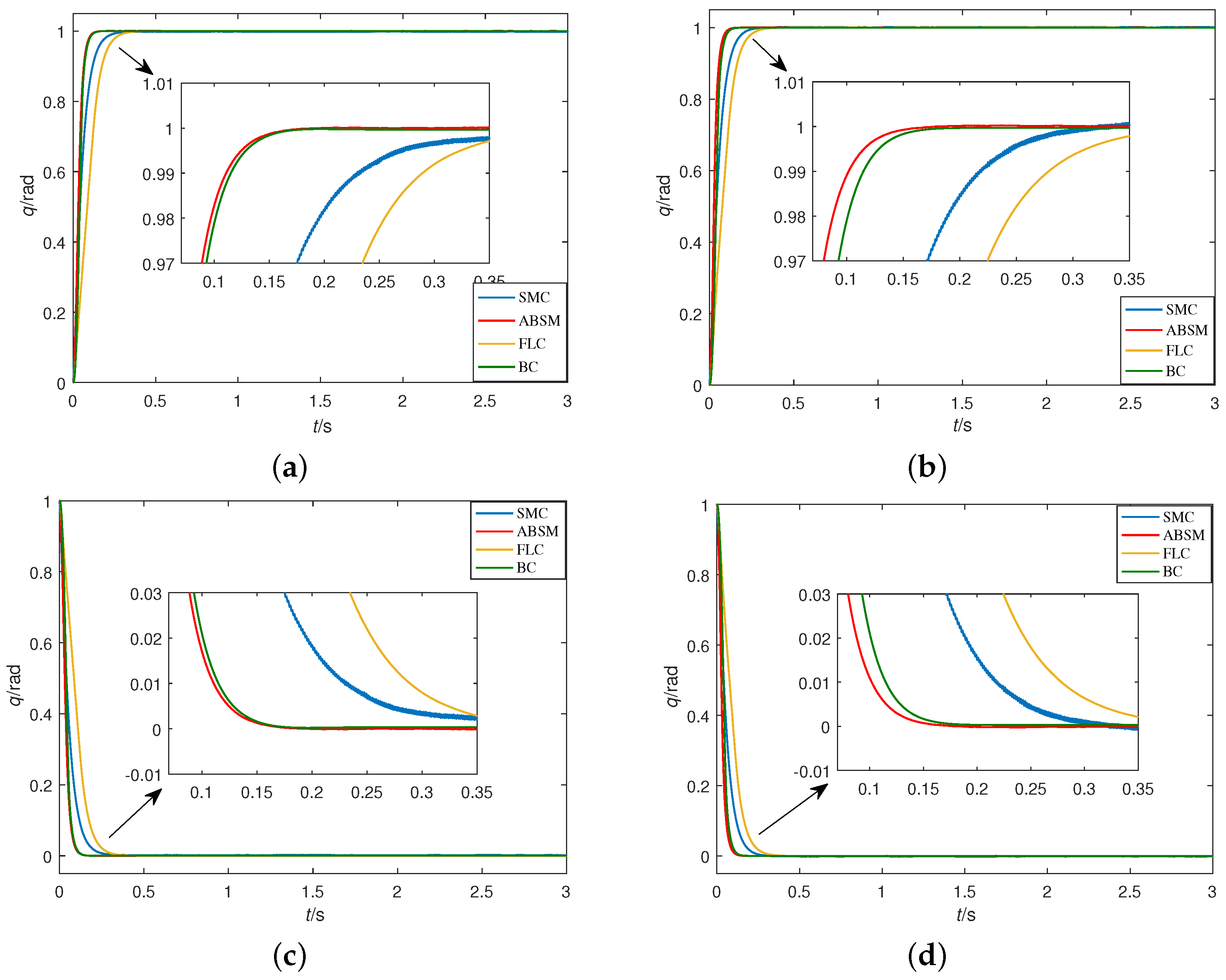
Case 1: To verify the advantage of the ABSM signal controller in dynamic response performance, simulations are conducted to compare the ABSM controller with BC, SMC, and feedback linearization control (FLC). Under no load condition, Joint 1 and Joint 2 track the unit step signal. The simulation results are shown in
Figure 5. The results indicate that the ABSM controller has the fastest dynamic response speed among the above four controllers. Therefore, the ABSM controller is the most suitable as the signal controller in the strategy of optimized cooperative control. The performance index of the four controllers is shown in
Table 4. It can be seen from
Table 4 that dynamic response time is the shortest when the ABSM controller is adopted.
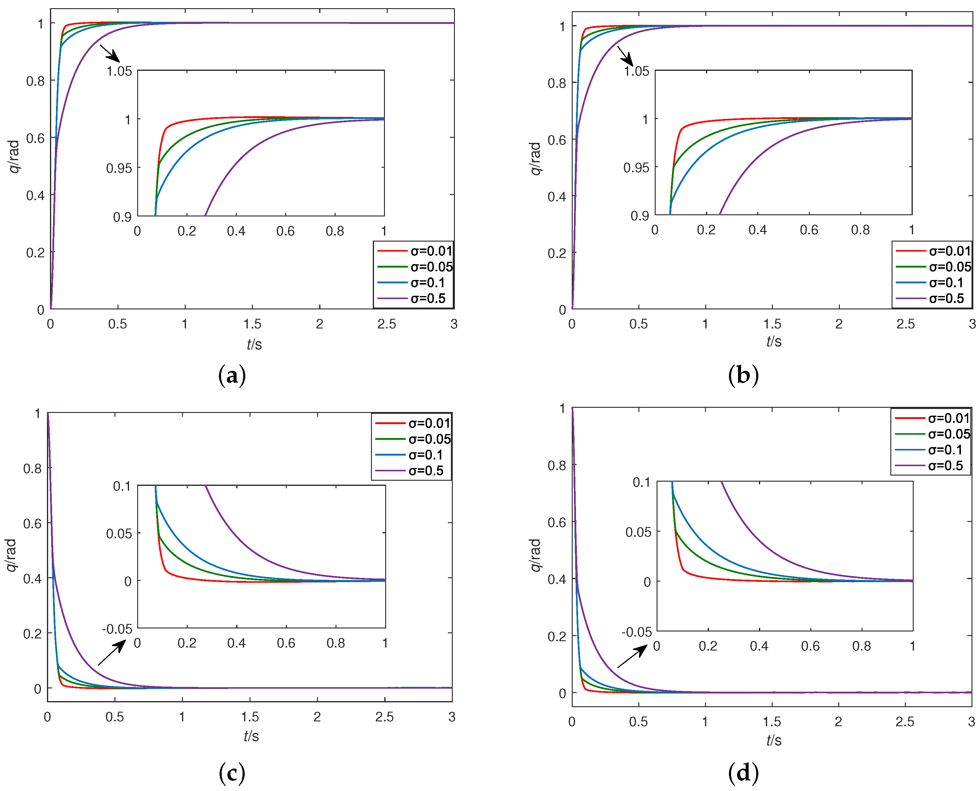
Case 2: To prove the effect of scale parameters on the cooperative control performance of the system, we select four groups of parameters:
,
,
and
. Robot joints track the unit step signal under the above four groups of parameters. The simulation results are shown in
Figure 6. It can be observed from
Figure 6 that the response speed of the system is the fastest with
. The steady-state error rates of the system are the same with different scale parameters. Furthermore, the smaller the scale parameter, the faster the response speed. Therefore, we choose the scale parameter
in the following
Case 3. In this case, the dynamic characteristics of the robot servo system are optimal.
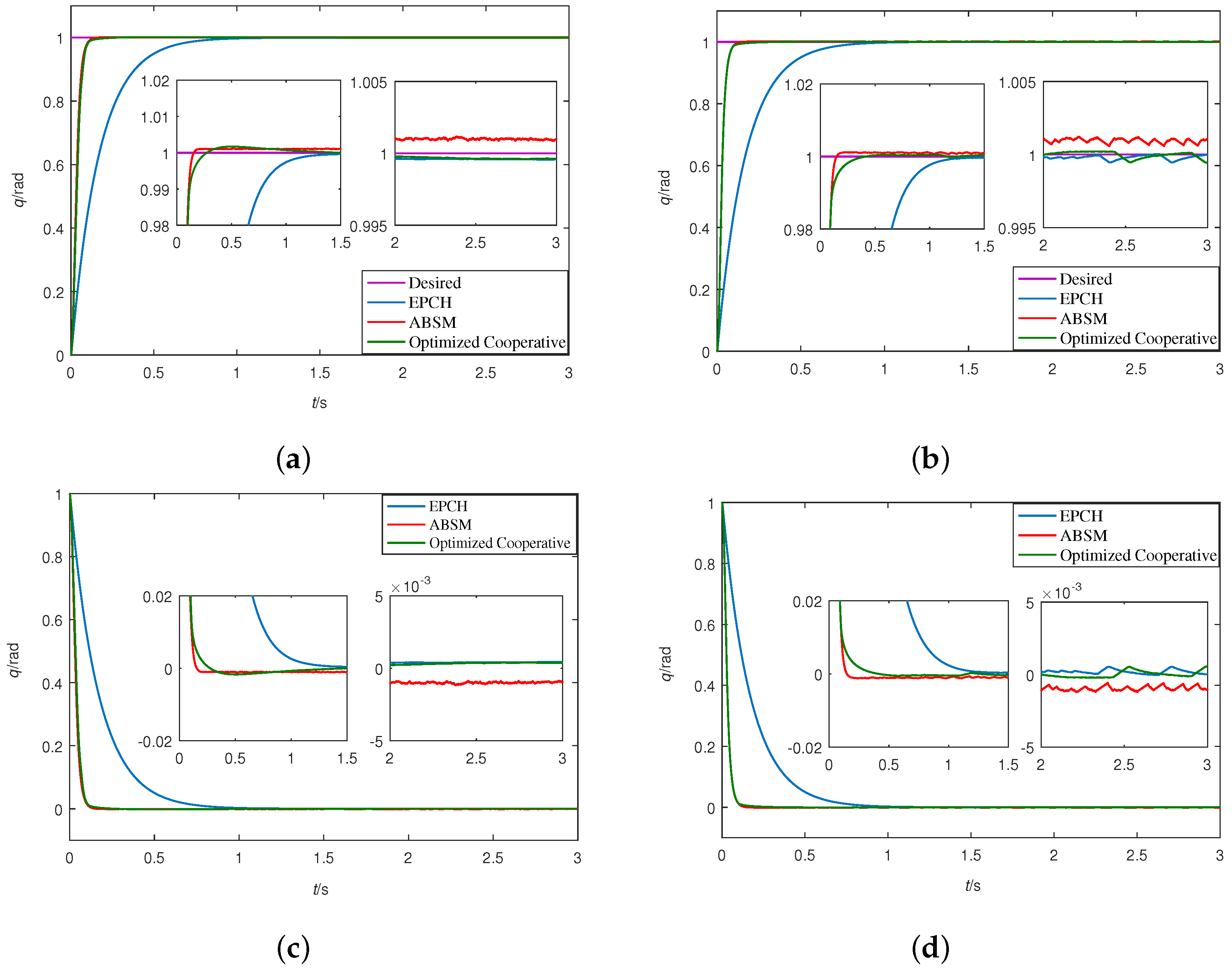
Case 3: To demonstrate the effectiveness of the strategy of optimized cooperative control, the curve of unit step response is measured. The scale parameter is set to
. The obtained curves of position tracking are displayed in
Figure 7. The simulation results reveal that the control characteristic after the application of optimized cooperative control is significantly better than with EPCH or ABSM. It can be seen from
Table 5 that, when the ABSM signal controller is used alone, the rise time of the system is about (0.17 s, 0.18 s) and the tracking error of the system is about (
rad,
rad); when the EPCH controller is used alone, the system’s rise time is about (1.02 s, 1.06 s) and its tracking error is about (
rad,
rad); when the strategy of optimized cooperative control is used, the system’s rise time is about (0.21 s, 0.23 s) and its tracking error is about (
rad,
rad). Therefore, the strategy of optimized cooperative control can reduce the rise time of the EPCH energy controller and the steady-state error of the ABSM signal controller. The optimized cooperative controller can give robot joints both superior rapidity and accuracy at once.
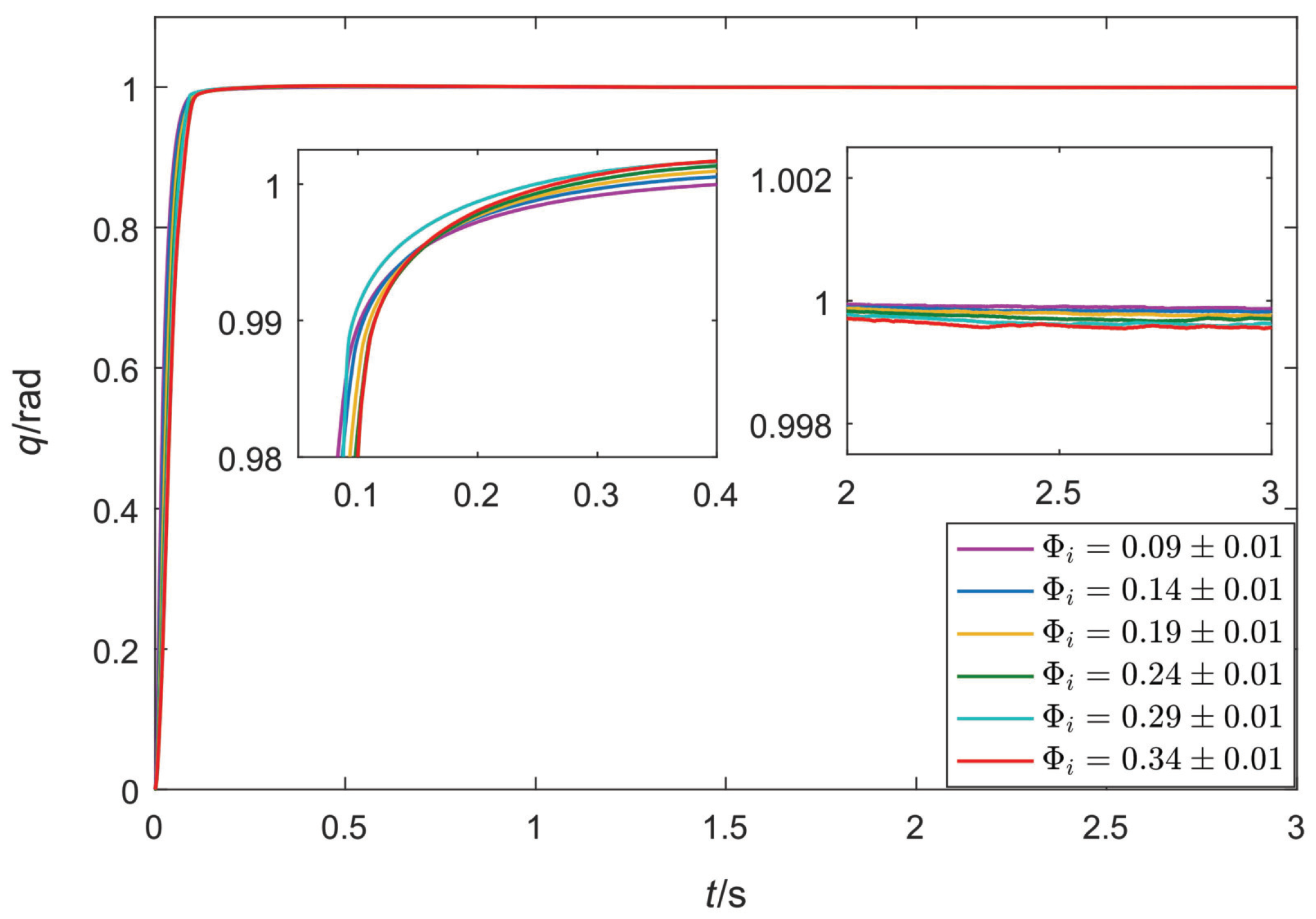
Case 4: To verify the influence of the PMSM mathematical model parameter
on the simulation results, the relevant parameter sensitivity analysis is shown in
Figure 8. The robot joint with optimized cooperative control tracks the unit step signal. The rise time required by the system is the lowest when
is selected; in this case, the system has the fastest dynamic response speed. However, a different PMSM mathematical model parameter
has almost the same effect on tracking error. Therefore, the system has the best control effect when
is adopted and the approximate error is
about
.


