Article

A Switching Mode Control Scheme for the Hovering Control of Quadrotor Unmanned Aerial Vehicles

1
College of Science, University of Shanghai for Science and Technology, Shanghai 200093, China
2
Department of Control Science and Engineering, University of Shanghai for Science and Technology, Shanghai 200093, China
*
Author to whom correspondence should be addressed.
These authors contributed equally to this work.
Mathematics 2023, 11(4), 994; https://doi.org/10.3390/math11040994
Submission received: 3 January 2023 / Revised: 6 February 2023 / Accepted: 13 February 2023 / Published: 15 February 2023

Abstract

:
This paper presents a novel switching mode control scheme for the six-DOF hovering control of underactuated quadrotor unmanned aerial vehicles (QUAVs) with strong coupling. Through this paper, the full six states of the position and attitude of the QUAV can be controlled to the special target configuration in a fixed time. First, a continuously differentiable fixed time controller with a state constraint was designed for the position system. Second, a fixed-time integral sliding mode controller was designed for the attitude subsystem. Thirdly, a switching law was designed to switch the above two types of controllers a limited number of times during hovering control. Additionally, the crash problem is fully discussed during the entire control process. In summary, the full-state hover mission was completed. The simulation experiments verify the effectiveness of the control algorithm.
MSC:
68T40; 70E60; 93B12; 93B53; 93C35; 93C85; 93D05; 34A34

1. Introduction

1.1. Background and Motivations

The quadrotor unmanned aerial vehicle (QUAV) is a kind of rotor micro-QUAV that combines the characteristics of nonlinearity, underactuation, strong coupling, and multivariability, etc. Its mechanical structure is simple, compact, and flexible, and it has important military and civil value [1]. Therefore, an increasing amount of scholars focus on the QUAV flight control, such as hovering control and tracking control. Among them, hovering control is one of the most basic and essential flight control methods for making the QUAV reach the target position first and then hovering in a specified attitude. For example, hovering control is indispensable for aerial performances or the delivery of goods using the QUAV in life. Therefore, it is valuable to design a controller with an excellent performance to control the QUAV to accomplish hovering tasks [2].
The QUAV can directly control the attitude angle and flight height by adjusting the rotational speeds of the four propellers during the flight, whereas the horizontal position can only be controlled indirectly through the coupling relationship between the QUAV attitude angle and the horizontal position. However, in addition to coupling and underactuation, external environments such as wind and magnetic fields can also affect the flight of the QUAV, which can lead to a crash event [3]. All of these factors make the design of a hovering controller for quadrotors challenging.
At present, many scholars have designed various controllers for the above problem, such as dual-loop controllers [4], robust backstepping controllers based on fuzzy compensation [5], and backstepping adaptive controllers (BACs) [6]. Although they can accomplish hover control to some extent, they are unable to control both the position and attitude to a specified configuration at the same time. Therefore, the focus of this paper is to design controllers with a superior performance to perform the hovering control of QUAVs while simultaneously reaching special positions and attitudes without crashing.

1.2. Literature Review

Up until now, a number of linear and nonlinear control methods have been reported to control quadrotor UAV flight control. With the development of artificial intelligence, some scholars proposed an artificial neural network (ANN) algorithm. An adaptive neural trajectory controller was set up to finish the control task in [7]. Rao et al. proposed a cascaded fuzzy neural net control method for position control that effectively reduces the overshoot and stabilization time [8]. Wang et al. proposed a non-singular fast terminal sliding mode control strategy to achieve the asymptotic stabilization of the error system [9]. Li et al. designed a generalized proportional integral observer-based finite-time composite control strategy that effectively solves the attitude deviation problem caused by wind disturbance [10]. However, these control methods can only achieve an asymptotic or finite-time stabilization of the system. Although the system state will eventually reach the equilibrium point, the convergence time cannot be determined, and its upper bound is related to the initial state, which will increase infinitely as the initial state tends to infinity. Both the uncertainty of the initial state and the infinity of time bring great obstacles to the application of control methods in practice.
To solve this problem, the concept of fixed-time stability was first proposed by Polyakov, which mainly shows that the convergence time of the system is only related to the system parameters and is independent of the initial state [11]. This important feature has laid an essential theoretical foundation for scholars to design fixed-time control algorithms that are more applicable in practical engineering. To better resist disturbances, a robust tracking control scheme based on a fixed-time perturbation observer was proposed in [12,13]. In [14], a combination of a fixed-time and sliding mode control observer was designed to effectively deal with ground effects and blade damage in the attitude subsystem. In [15], an active fault-tolerant control scheme based on fixed-time linear self-anti-disturbance control was designed. Based on the homogeneity theory and the Lyapunov stability method, a double-loop fixed-time controller was designed for attitude control in [16]. Based on the design idea of internal and external separation, a fixed-time output feedback trajectory tracking control strategy was designed by [17]. However, the influence of the altitude constraint existing in the flight control process of the QUAV has been neglected in all of the previous papers.
In fact, due to the coupling nature of the QUAV system, the altitude will keep changing with other states during the flight. Therefore, the control process should ensure that its flight altitude is always higher than the safety altitude; otherwise, it may make the QUAV crash. However, the current literature on the flight control of QUAVs hardly considers it, except for [18], which designs a trajectory optimization algorithm based on the Gaussian pseudospectral method of altitude that gives an altitude constraint. However, it should be noted that this work is not fixed time, which means that the convergence time has uncertainty. For this shortcoming, the fixed-time control algorithm with constraints is considered in this paper.
It is well known that sliding mode control algorithms play a significant role in the control of nonlinear systems. Therefore, many scholars have combined fixed-time theory with sliding mode control and proposed various new control strategies. Based on the appointed fixed-time sliding mode variables and adaptive techniques, an improved adaptive sliding mode law was designed [19]. A flatness-based fixed-time sliding mode control strategy was proposed for the quadrotor trajectory tracking problem subject to external disturbances [20]. A new continuous non-singular terminal sliding mode control was designed so that the sliding motion was fixed-time stable and not affected by the initial conditions of the system [21]. Ref. [22] proposed a new integral-type sliding mode adaptive technique based on fixed-time control law to suppress system perturbations and actuator failures. However, this work only considers the attitude angle control and ignores the importance of position control. Further studies will be seen in this research.
To be able to control more states of this multivariable system, and to better accomplish the control tasks, scholars must fully analyze the model structure of the QUAV. The original system can be seen as a dynamic system that is composed of two subsystems: one is a dynamic subsystem composed of three position variables, and the other is a dynamic subsystem composed of three angle variables. A non-singular fast terminal sliding mode control (NFTSMC) algorithm was designed in [23] based on the extended state observer (ESO) in order to complete the control task of three attitude angles, but the position control was not analyzed. Researchers carried out further research, and a novel adaptive robust control approach was proposed that can realize altitude control based on attitude angle control [24]. In reality, position control is very essential for hovering. Because the attitude subsystem can be decoupled into three attitude angle subsystems for separate control, attitude control is relatively easy. In contrast, for the position subsystem, three position coordinates have only one control input, and when the attitude angle changes, the position coordinates also change; thus, it is difficult to complete the control task of the three states of the position. Therefore, scholars have fully analyzed the coupling between the position and the attitude angle, and they have finally realized that a total of four states of the position and yaw angle can be controlled to a target value [21,25,26]. However, the roll angle and pitch angle cannot be freely controlled due to coupling, and they can only be controlled to certain unknown angles, which are derived from the position controller [27,28,29]. In order to overcome this challenge, this research starts from hovering control and combines the theory of homogeneity with the fixed-time control method to conduct a deep study. According to the requirement of stability, the conditions where six configuration variables can be completely stabilized are given in this research. Then, it is devoted to designing a new scheme for solving six state control problems of QUAVs.

1.3. Contribution

Motivated by the above research on QUAV control algorithms, this paper implements six-DOF hovering control for a given desired posture in a fixed time. The main contributions are as follows.
(1)
The position and attitude control of the QUAV achieve simultaneous stability. Different from the article [30], which only achieves the asymptotic stabilization of the position and yaw angle four-state control error system, the algorithm designed in this paper can completely control the configuration of the QUAV so as to realize hovering in a finite time at the equilibrium point that can be simultaneously stabilized.
(2)
A novel switching mode control algorithm is designed. Compared with the work in [31], which only analyzes the position and attitude subsystems separately, this paper not only analyzes the overall system control process in detail but also realizes the full-state control of the position and attitude to the target posture.
Furthermore, this switching control method consists of a fixed-time controller with constraints and a fixed-time integral sliding mode controller (FTISMC), which has never been designed in UAV control before. Compared with [32], in addition to allowing the system to achieve fixed-time stability, it also ensures that the altitude always meets the no-crash requirement, and further improves the control performance by eliminating the steady-state error with the help of the integral term.
(3)
To avoid a crash, the altitude change of the QUAV during the whole flight control process is analyzed in detail. The second-order differentiable fixed-time control algorithm with constraints is designed in the position loop to avoid the crash effectively.

1.4. Paper Organization

The paper is organized as follows: The QUAV system model, the research questions, and some necessary preliminaries are proposed in Section 2. The controller design details and stability analysis are given in Section 3. Simulations and comparative tests are performed in Section 4. The conclusions are given in Section 5. In addition, some important lemmas and proofs are presented in the Appendix A.
Notations: Throughout this paper, for a vector x = ( x 1 , , x n ) T R n , we denote x ¯ j = ( x 1 , , x j ) T R j , j = 1 , , n . For any a > 0 and x R , the function x a is defined as x a = x a for x > 0 ; x a = 0 for x = 0 ; x a = | x | a for x < 0 ; and the function x a is defined as x a = | x | a s i g n ( x ) , where:
s i g n ( x ) = 1 , x > 0 1 , 1 , x = 0 1 , x < 0 .
The value of s i g n ( x ) takes a random value of between 1 , 1 when x = 0 . Furthermore, for the convenience of writing, the arguments of the functions are omitted whenever no confusion arises in the context.

2. Model Description and Problem Formulation

2.1. Model of QUAVs

The QUAV is an underactuated system with four inputs and six outputs. The theoretical model of a QUAV is shown in Figure 1, which establishes the ground coordinate system and the body-fixed coordinate system. The earth-based coordinate system {E} ( O e , x e , y e , z e ) and the body-fixed coordinate system {B} ( O b , x b , y b , z b ) are introduced to describe the position { x , y , z } and the attitude angles { ϕ , θ , ψ } of the QUAV. In addition, the power system of the drone mainly consists of four micro-motors and propellers [33]. This subsection combines physical laws and mathematical methods to model the dynamics of the QUAV.
Define the angular velocities of the four rotors as ω 1 , ω 2 , ω 3 , ω 4 ; the total lift in the z b direction as U 1 , and the torques around the body frame axis as U 2 , U 3 , and U 4 [34].
U 1 ( t ) = b m ( ω 1 2 ( t ) + ω 2 2 ( t ) + ω 3 2 ( t ) + ω 4 2 ( t ) ) , U 2 ( t ) = l b J x ( ω 2 2 ( t ) + ω 4 2 ( t ) ) , U 3 ( t ) = l b J y ( ω 1 2 ( t ) + ω 3 2 ( t ) ) , U 4 ( t ) = d J z ( ω 1 2 ( t ) + ω 2 2 ( t ) ω 3 2 ( t ) + ω 4 2 ( t ) ) ,
where m is the mass, b denotes the lift coefficient, d denotes the antitorque coefficient, and l is the length of the quadrotor arm. J x , J y , and J z are the moments of inertia in Table 1.
In order to simplify the problem, the external inference factors such as the air resistance and gyro effect are ignored. Considering the QUAV as a rigid body and its structure as symmetrical, the model of QUAV can be obtained as in [21,35]:
x ¨ = U 1 ( c o s ϕ s i n θ c o s ψ + s i n ϕ s i n ψ ) , y ¨ = U 1 ( c o s ϕ s i n θ s i n ψ s i n ϕ c o s ψ ) , z ¨ = U 1 c o s ϕ c o s θ g , ϕ ¨ = 1 J x ( J y J z ) θ ˙ ψ ˙ + U 2 , θ ¨ = 1 J y ( J z J x ) ϕ ˙ ψ ˙ + U 3 , ψ ¨ = 1 J z ( J x J y ) ϕ ˙ θ ˙ + U 4 ,
where x , y , and z represent the position in the inertial frame; g is the gravity coefficient; and ϕ , θ , and ψ represent the roll angle, pitch angle, and yaw angle, respectively.
To simplify the dynamics model, the following definitions are introduced:
x 1 = ϕ ( t ) , x 2 = ϕ ˙ ( t ) , x 3 = θ ( t ) , x 4 = θ ˙ ( t ) , x 5 = ψ ( t ) , x 6 = ψ ˙ ( t ) , x 7 = x ( t ) , x 8 = x ˙ ( t ) , x 9 = y ( t ) , x 10 = y ˙ ( t ) , x 11 = z ( t ) , x 12 = z ˙ ( t ) .
Thus, the model of the QUAV (2) can be rewritten as follows:
ϕ ¨ = x ¨ 1 = x ˙ 2 = a 1 x 4 x 6 + U 2 , θ ¨ = x ¨ 3 = x ˙ 4 = a 2 x 2 x 6 + U 3 , ψ ¨ = x ¨ 5 = x ˙ 6 = a 3 x 2 x 4 + U 4 , x ¨ = x ¨ 7 = x ˙ 8 = U 1 ( c o s x 1 s i n x 3 c o s x 5 + s i n x 1 s i n x 5 ) , y ¨ = x ¨ 9 = x ˙ 10 = U 1 ( c o s x 1 s i n x 3 s i n x 5 s i n x 1 c o s x 5 ) , z ¨ = x ¨ 11 = x ˙ 12 = U 1 c o s x 1 c o s x 3 g ,
where a i are the standard parameters for i = 1 , 2 , 3 , and
a 1 = J y J z J x , a 2 = J z J x J y , a 3 = J x J y J z .

2.2. Problem Formulation

In this research, the hovering problem of special postures is fully considered. The reports in [30,31,36] also study the QUAV hover control problem and accomplish the task of controlling a total of four states of the position and yaw angles to the target attitude. However, the roll angle and pitch angle are limited by the output of the position controller and cannot be freely controlled. Therefore, the control objective of this research is to design a controller that generates torque to allow the position and attitude of QUAV to hover steadily in the desired position and attitude. In addition, in order to ensure that the UAV will not fall from a high place to the ground, the safe flight height H 0 is given. It is required that the flight altitude of the four-rotor UAV is always greater than the given safe altitude; that is, there will be no crash.
Give the desired trajectory { x T , y T , z T , ϕ T , θ T , ψ T } . Since hovering is in a fixed posture, the desired trajectory is a constant. By using Equation (3), it is clear that the control errors in the position loop and attitude loop can be defined as Equation (5), respectively:
e 1 ( t ) = x 1 ( t ) ϕ T , e 2 ( t ) = x 2 ( t ) , e 3 ( t ) = x 3 ( t ) θ T , e 4 ( t ) = x 4 ( t ) , e 5 ( t ) = x 5 ( t ) ψ T , e 6 ( t ) = x 6 ( t ) , e 7 ( t ) = x 7 ( t ) x T , e 8 ( t ) = x 8 ( t ) , e 9 ( t ) = x 9 ( t ) y T , e 10 ( t ) = x 10 ( t ) , e 11 ( t ) = x 11 ( t ) z T , e 12 ( t ) = x 12 ( t ) .
Therefore, the control objective is to design a controller so that the errors converge to zero in a fixed time with no crash, i.e., e i converges to zero in a fixed time for i = 1 , 2 , , 12 , and no crash.

3. Controller Design and Stability Analysis

It is known that the QUAV system (4) is controllable according to the literature [37] controllability proof. It is easy to see from the form of the system (4) that the states of the three attitude angle equations are completely controllable, and that it is not difficult to control them. The difficulty is that there is only one control input U 1 for the three position coordinate equations, which are nonlinear coupled by the sine cosine of the three attitude angles. It may need to be maintained at three special attitude angles to become controllable. Therefore, our control idea is to design a switching rate, switching back and forth between three position equation controls and the three attitude equation controls, and finally achieving the given value of six position and attitude variables.
Next, the control laws of the two subsystems are designed, respectively, and then the switching law is designed.

3.1. Controller Design of the Position Subsystem

First, we will discuss what position and attitude the QUAV can hover at. Second, we will discuss how to satisfy this condition. Third, if the condition is satisfied, we will determine how to design the controller U 1 in order to make the three position coordinates converge to the ideal value in a fixed time.
First, the problem of QUAV hovering to a position is considered. The desired fixed position { x T , y T , z T } is presented. Obviously, x ˙ T = y ˙ T = z ˙ T = 0 . Using Equations (4) and (5), it can be obtained that the control errors of the position subsystem can be expressed as:
e ˙ 7 = e 8 , e ˙ 8 = U 1 ( c o s ϕ s i n θ c o s ψ + s i n ϕ s i n ψ ) , e ˙ 9 = e 10 , e ˙ 10 = U 1 ( c o s ϕ s i n θ s i n ψ s i n ϕ c o s ψ ) , e ˙ 11 = e 12 , e ˙ 12 = U 1 c o s ϕ c o s θ g .
The equilibrium of the dynamic system above must meet:
U 1 ( c o s ϕ s i n θ c o s ψ + s i n ϕ s i n ψ ) = 0 , U 1 ( c o s ϕ s i n θ s i n ψ s i n ϕ c o s ψ ) = 0 , U 1 c o s ϕ c o s θ g = 0 .
According to Equation (7), it is easily seen that U 1 0 and Equation (8) can be obtained.
c o s ϕ s i n θ c o s ψ + s i n ϕ s i n ψ = 0 , c o s ϕ s i n θ s i n ψ s i n ϕ c o s ψ = 0 .
The two equations of Equation (8) are equivalent to s i n ϕ = 0 and s i n θ = 0 . It can be concluded that ϕ = θ = 0 or ϕ = θ = k π , where k is an integer. This means that the true values of ϕ and θ must be zero when hovering. In other words, if the hovering angles of the ϕ and θ ideals given in advance are not zero, it is impossible to achieve the e 7 and e 9 convergence to zero. Therefore, the ideal attitude angles given by the hovering of the QUAV must meet ϕ = 0 and θ = 0 . ψ is not limited. In summary, this means that the attitude angle of this kind of QUAV when hovering must be { ϕ T , θ T , ψ T } = { 0 , 0 , ψ T } .
The control problem of the position control subsystem (6) is discussed below.
For the position error subsystem (6), the virtual control input signals a ( t ) , b ( t ) , and c ( t ) in the x , y , and z directions are defined:
a ( t ) = U 1 ( c o s ϕ s i n θ c o s ψ + s i n ϕ s i n ψ ) , b ( t ) = U 1 ( c o s ϕ s i n θ s i n ψ s i n ϕ c o s ψ ) , c ( t ) = U 1 c o s ϕ c o s θ g .
If a ( t ) , b ( t ) , and c ( t ) can be designed arbitrarily, the system (6) is a state that is a fully controllable system composed of three fully decoupled second-order integrators. Their fixed-time control is not difficult to obtain.
 Theorem 1.
Consider the position error subsystem (6) with Equation (9); then, give the set Ω = { w | w R , | w | < σ } , where σ is a positive constant. If the continuous fixed-time controllers are set as:
a ( t ) = 0 t d τ 0 τ ( β 4 x ( z ¯ 4 x ) ζ 4 x r 5 x d s , b ( t ) = 0 t d τ 0 τ ( β 4 y ( z ¯ 4 y ) ζ 4 y r 5 y d s , c ( t ) = 0 t d τ 0 τ ( β 4 z ( z ¯ 4 z ) ζ 4 z r 5 z d s ,
where the parameters r 5 x , r 5 y , and r 5 z ; functions β 4 x ( · ) , β 4 y ( · ) , β 4 z ( · ) , ζ 4 x , ζ 4 y ; ζ 4 z are selected as given in Lemma A1 in Appendix A.1; and z i x , z i y , and z i z denote the i 1 -th-order derivative of the position errors e 7 ( t ) , e 9 ( t ) , and e 11 ( t ) , respectively; then, for all initial values e 7 ( 0 ) , e 9 ( 0 ) , e 11 ( 0 ) Ω , the following properties are established.
(i) 
The states e 7 ( t ) , e 9 ( t ) , and e 11 ( t ) all stay in the sets Ω for any t 0 , respectively.
(ii) 
The position error e i ( t ) , i = 7 , 8 , , 12 is regulated to zero in a fixed settling time T.
See Appendix A.3 for the proof of Theorem 1.
 Remark 1.
In some references, Equation (10) is often written in the following form:
a ( t ) = β 4 x ( z ¯ 4 x ) ζ 4 x r 5 x , b ( t ) = β 4 y ( z ¯ 4 y ) ζ 4 y r 5 y , c ( t ) = β 4 z ( z ¯ 4 z ) ζ 4 z r 5 z .
None of the above three expressions can be differentiated, especially at the origin, or are even discontinuous. When the QUAV is controlled to the ideal position, the angle of the QUAV is required to be controlled to the attitude angle, which requires that it is second-order steerable. Thus, here, we use the second integral.
 Remark 2.
The controller designed in comparison [35] is discontinuous, and the virtual control law designed in this paper is continuous and differentiable, which lays the foundation for the smoothness required for the attitude angle to reach a special attitude angle.
The above theorem shows that if the virtual controller can be designed as a ( t ) , b ( t ) , and c ( t ) , as defined in Equation (10), the hovering of three position coordinates can be completed. The following discusses what kind of situation a ( t ) , b ( t ) , and c ( t ) can be designed in order to look like Equation (10). Consider the necessity first.
Assuming that a ( t ) , b ( t ) , and c ( t ) are given according to Equation (10), consider whether U 1 ( t ) , ϕ ( t ) , θ ( t ) , and ψ ( t ) can satisfy Equation (9). According to the mathematical derivation, Equation (9) is equivalent to Equation (11).
a c o s ψ + b s i n ψ = U 1 c o s ϕ s i n θ , a s i n ψ b c o s ψ = U 1 s i n ϕ , c + g = U 1 c o s ϕ c o s θ .
For a given a ( t ) , b ( t ) , and c ( t ) , they depend only on the position and their derivative information, and are independent of the angle variable. We will consider how U 1 ( t ) , ϕ ( t ) , θ ( t ) , and ψ ( t ) satisfy Equation (11).
 Proposition 1.
Equation (11) has a solution in the following form.
U 1 ( t ) = a 2 + b 2 + ( c + g ) 2 , ϕ d ( t ) = 0 , θ d ( t ) = a t a n 2 ( a 2 + b 2 U 1 , c + g U 1 ) , ψ d ( t ) = a t a n 2 ( b a 2 + b 2 , a a 2 + b 2 ) .
The properties of the arctangent function are described in Appendix A.2, Property A1. Additionally, see Appendix A.4 for the proof of Proposition 1.
The above proposition shows that, as U 1 ( t ) is designed according to Equation (12), U 2 ( t ) , U 3 ( t ) , and U 4 ( t ) can be designed so that ϕ ( t ) , θ ( t ) , and ψ ( t ) are equal to the three angles ϕ d ( t ) , θ d ( t ) , and ψ d ( t ) , respectively, given by Equation (12) within a fixed time. After that time, Equation (11) is established, and, thus, Equation (9) is established. In this way, if a ( t ) , b ( t ) , and c ( t ) are provided by Equation (10), it can be seen from Theorem 1 that the position errors of the three position coordinates converge to zero in a fixed time.
 Remark 3.
Compared to the virtual control inputs designed in [25,38], which are not second-order differentiable, the virtual control inputs a ( t ) , b ( t ) , and c ( t ) designed in this work are continuously second-order differentiable. Therefore, the target attitude angles θ d ( t )   a n d   ψ d ( t ) are also continuously second-order differentiable, which lays the foundation for subsequent attitude control.
According to the above analysis, in the flight control process, the three attitude angles ϕ ( t ) , θ ( t ) , and ψ ( t ) should be controlled to ϕ d ( t ) , θ d ( t ) , and ψ d ( t ) in a fixed time, as shown in Equation (12) at first. Each of the three attitude angles is a second-order system relative to its control input. In order to control the three angles to an ideal value of ϕ d ( t ) , θ d ( t ) , and ψ d ( t ) , respectively, the second derivative of ϕ d ( t ) , θ d ( t ) , and ψ d ( t ) with respect to time must exist. The previous research only noticed that seeking a solution of the equation system (11), i.e., the form of (12), did not consider that the subsequent control implementation requires a second derivative, which is the reason for why we propose a double-integral fixed-time controller (10) in the article.
Next, consider how to design U 1 ( t ) , U 2 ( t ) , U 3 ( t ) , and U 4 ( t ) so that the three attitude angles can reach the desired attitude angles satisfying Equation (12) in a fixed time.

3.2. Controller Design of the Attitude Subsystem

In this subsection, the fixed-time integral sliding mode controller is designed to complete the attitude angle tracking control task. U 1 ( t ) is designed according to Equation (12). Now, consider the design problem for U 2 ( t ) , U 3 ( t ) , and U 4 ( t ) .
Consider three expected attitude angles ϕ d ( t ) , θ d ( t ) , and ψ d ( t ) , which satisfy Equation (12). The dynamic equation of the attitude angle error can be expressed based on Equations (4) and (5) as follows:
e ˙ 1 = x ˙ 1 ϕ ˙ d = e 2 , e ˙ 2 = x ¨ 1 ϕ ¨ d = a 1 x 4 x 6 + U 2 ϕ ¨ d , e ˙ 3 = x ˙ 3 θ ˙ d = e 4 , e ˙ 4 = x ¨ 3 θ ¨ d = a 2 x 2 x 6 + U 3 θ ¨ d , e ˙ 5 = x ˙ 5 ψ ˙ d = e 6 , e ˙ 6 = x ¨ 5 ψ ¨ d = a 3 x 2 x 4 + U 4 ψ ¨ d .
For the attitude error subsystem (13), define the following integral sliding surfaces as:
s e 1 ( t ) = e 2 ( t ) + k 1 0 t ( e 1 ( τ ) ϱ 1 + e 1 ( τ ) + e 1 ( τ ) ϱ 1 ) d τ + k 2 0 t ( e 2 ( τ ) ϱ 2 + e 2 ( τ ) + e 2 ( τ ) ϱ 2 ) d τ , s e 3 ( t ) = e 4 ( t ) + k 3 0 t ( e 3 ( τ ) ϱ 3 + e 3 ( τ ) + e 3 ( τ ) ϱ 3 ) d τ + k 4 0 t ( e 4 ( τ ) ϱ 4 + e 4 ( τ ) + e 4 ( τ ) ϱ 4 ) d τ , s e 5 ( t ) = e 6 ( t ) + k 5 0 t ( e 5 ( τ ) ϱ 5 + e 5 ( τ ) + e 5 ( τ ) ϱ 5 ) d τ + k 6 0 t ( e 6 ( τ ) ϱ 6 + e 6 ( τ ) + e 6 ( τ ) ϱ 6 ) d τ ,
where the parameters k i , ϱ i , and ϱ i , ( i = 1 , , 6 ) are selected as given in Appendix A.1, Lemma A2.
To solve this tracking problem, the following fixed-time sliding mode control scheme is developed.
 Theorem 2.
Considering the attitude error subsystem (13), the following fixed-time integral sliding mode controllers are set as:
U 2 ( t ) = k 1 ( e 1 ϱ 1 + e 1 + e 1 ϱ 1 ) k 2 ( e 2 ϱ 2 + e 2 + e 2 ϱ 2 ) k 1 ( s e 1 1 + 1 μ + s e 1 + s e 1 1 1 μ ) a 1 x 4 x 6 + ϕ ¨ d , U 3 ( t ) = k 3 ( e 3 ϱ 3 + e 3 + e 3 ϱ 3 ) k 4 ( e 4 ϱ 4 + e 4 + e 4 ϱ 4 ) k 3 ( s e 3 1 + 1 μ + s e 3 + s e 3 1 1 μ ) a 2 x 2 x 6 + θ ¨ d , U 4 ( t ) = k 5 ( e 5 ϱ 5 + e 5 + e 5 ϱ 5 ) k 6 ( e 6 ϱ 6 + e 6 + e 6 ϱ 6 ) k 5 ( s e 5 1 + 1 μ + s e 5 + s e 5 1 1 μ ) a 3 x 2 x 4 + ψ ¨ d ,
where ρ > 0 and μ > 1 are constants, such that the origin of system (13) is fixed-time stable for any initial condition.
 Remark 4.
From the composition of the above three controllers, we can see that, here, the second derivatives of ϕ d , θ d , and ψ d with respect to time are required. It can be deduced from (12) that the second derivative of a , b , and c is also required. This is the reason for why we use the double integral in Equation (10) of Theorem 1: because the integrand of Equation (10) is not differentiable. However, many previous studies only used the (10) integrand as virtual control inputs, which are difficult to implement in practice.
 Proof. 
Due to the symmetry, we only need to prove that e 1 and e 2 meet the conclusion of the theorem. The proof consists of two steps. We first show that the system can reach s e 1 = 0 in a fixed time under the controller (15). Then, we will prove that the tracking errors e 1 and e 2 converge to zero in a fixed time during the sliding motion s e 1 = 0 .
(1) The candidate Lyapunov function of the ϕ -subsystem is considered as:
V ( e 1 ) = | s e 1 | .
It is worth noting that the definition of V ˙ becomes nontrivial when s e 1 = 0 . This is because the right-hand side of (16) becomes discontinuous. Then, the concepts of Filippov solutions and the set-valued Lie derivative need to be applied [39]. Then, we have:
V ˙ s i g n ( s e 1 ) s ˙ e 1 | s e 1 S 0 + s i g n ( s e 1 ) s ˙ e 1 | s e 1 S 1 ,
where S 0 = s e 1 = 0 and S 1 = s e 1 0 are two sets. In the sense of Filippov, the case in which s e 1 = 0 holds for isolated time instants with zero measure can be disregarded in these time instants. If s e 1 = 0 holds along an interval of time with positive measure, then s ˙ e 1 = 0 holds at these time instants. Thus, the time derivative of V can be evaluated as:
V ˙ = s i g n ( s e 1 ) s ˙ e 1 .
Considering the integral sliding surface s e 1 in Equation (14), we obtain:
V ˙ = s i g n ( s e 1 ) s ˙ e 1 = s i g n ( s e 1 ) ( e ˙ 2 + k 1 ( e 1 ϱ 1 + e 1 + e 1 ϱ 1 ) + k 2 ( e 2 ϱ 2 + e 2 + e 2 ϱ 2 ) ) = s i g n ( s e 1 ) ( a 1 x 4 x 6 + U 2 ϕ ¨ d + k 1 ( e 1 ϱ 1 + e 1 + e 1 ϱ 1 ) + k 2 ( e 2 ϱ 2 + e 2 + e 2 ϱ 2 ) ) .
Substituting U 2 into Equation (17) yields:
V ˙ = k 1 ( | s e 1 | 1 + 1 μ + | s e 1 | + | s e 1 | 1 1 μ ) k 1 ( | s e 1 | 1 + 1 μ + | s e 1 | 1 1 μ ) k 1 V 1 + 1 μ k 1 V 1 1 μ .
From Lemma A3 in Appendix A.1, the system will reach the sliding surface s i = 0 in a fixed time T r , where T r π μ 2 k 1 .
(2) When s e 1 0 , s ˙ e 1 = 0 can be obtained and the reduced close-loop dynamics for t T r can be deduced as:
e ˙ 1 = e 2 , e ˙ 2 = k 1 ( e 1 ϱ 1 + e 1 + e 1 ϱ 1 ) k 2 ( e 2 ϱ 2 + e 2 + e 2 ϱ 2 ) .
According to Lemma A2 in Appendix A.1, system (19) is fixed-time stable at the origin, i.e., there exists a constant T s that is independent of the initial conditions, such that e i 0 for all t T r + T s , i = 1 , 2 .
Thus, the tracking errors of the roll angle ϕ converge to zero and remain zero at a fixed time T ϕ T r + T s .
Similar to the above proof, it can be proven that the proposed controllers also guarantee the QUAV to track its desired trajectory in the θ and ψ attitude channels. □
For the three-attitude angle tracking subsystems composed of Equation (13), (14), and (15), there must exist a fixed time T = m a x { T ϕ , T θ , T ψ } so that the tracking errors have e i 0 , i = 1 , , 6 as t > T .

3.3. Switching the Control Law for the Full Closed Loop

In the previous two sections, the control laws of the position subsystem and attitude subsystem are designed, respectively, which can make QUAV realize the position and attitude control. However, the position error tracking can be completed only when three special attitude angles are required, and these special attitude angles are not necessarily the ideal attitude angles that we want. The ideal attitude angle cannot achieve the convergence of the position tracking error. Therefore, it is necessary to design a switching rate between the two subsystems to realize the final and complete simultaneous tracking of all six pose variables.
It is easy to know that, in the overall control of QUAV position and attitude, the altitude is always changing, and it is very likely to crash during descent. Therefore, it is necessary to analyze whether the QUAV will crash in the process of altitude change. Given the safe take-off height H 0 , the initial take-off altitude of the QUAV satisfies z ( 0 ) H 0 . Additionally, the desired altitude z T is always higher than the safe take-off altitude H 0 . Then, it is convenient to derive the following proposition.
 Proposition 2.
If the initial height error e 11 ( 0 ) meets | e 11 ( 0 ) | < z T H 0 , then the QUAV will not crash during flight under the control of controller (10).
 Proof. 
Firstly, considering the following altitude subsystem:
e ˙ 11 ( t ) = e 12 ( t ) , e ˙ 12 ( t ) = c ( t ) .
It follows from Theorem 1 that the state e 11 ( t ) of system (20) always satisfies the state constraint under the control of controller (10). Therefore, when the initial height error e 11 ( 0 ) has:
| e 11 ( 0 ) | = | z ( 0 ) z T | < z T H 0 ,
σ = z T H 0 . According to Theorem 1, the height error e 11 ( t ) always satisfies:
| e 11 ( t ) | = | z ( t ) z T | < z T H 0 , t 0 .
Equation (21) is equivalent to:
z ( t ) z T < z T H 0 , z T z ( t ) < z T H 0 .
Thus, it is easy to obtain H 0 < z ( t ) < 2 z T H 0 , which makes the QUAV altitude meet the condition of no crash during flight.
The proof is completed. □
Through the above analysis, we can find that the selection of H 0 is very important. If the given QUAV fuselage height is H b , the safe take-off height H 0 should meet H b H 0 < z T . The initial take-off height z ( 0 ) should meet z ( 0 ) H 0 . Therefore, in order to prevent the initial take-off height from being too high to be realized, H 0 should not be selected as too large a value.
Based on the above analysis, the switching controller is designed in the following three steps.
Step 1: For the given ideal positions x T , y T , and z T , e 7 , e 8 , , e 12 are defined according to Equation (5); a , b , and c are defined according to Theorem 1, U 1 ; ϕ d , θ d , and ψ d are defined according to Equation (12); and s e 1 , s e 2 , and s e 3 are specified by (14). U 2 , U 3 , and U 4 are given by (15). Taking control law (23), where e 1 , e 2 , , e 6 are defined according to Equation (13),
U 1 ( t ) = a 2 + b 2 + ( c + g ) 2 , U 2 ( t ) = k 1 ( e 1 ϱ 1 + e 1 + e 1 ϱ 1 ) k 2 ( e 2 ϱ 2 + e 2 + e 2 ϱ 2 ) k 1 ( s e 1 1 + 1 μ + s e 1 + s e 1 1 1 μ ) ρ s i g n ( s e 1 ) a 1 x 4 x 6 + ϕ ¨ d , U 3 ( t ) = k 3 ( e 3 ϱ 3 + e 3 + e 3 ϱ 3 ) k 4 ( e 4 ϱ 4 + e 4 + e 4 ϱ 4 ) k 3 ( s e 3 1 + 1 μ + s e 3 + s e 3 1 1 μ ) ρ s i g n ( s e 3 ) a 2 x 2 x 6 + θ ¨ d , U 4 ( t ) = k 5 ( e 5 ϱ 5 + e 5 + e 5 ϱ 5 ) k 6 ( e 6 ϱ 6 + e 6 + e 6 ϱ 6 ) k 5 ( s e 5 1 + 1 μ + s e 5 + s e 5 1 1 μ ) ρ s i g n ( s e 5 ) a 3 x 2 x 4 + ψ ¨ d .
It is well known that the QUAV drops from time to time. In the process of U 2 , U 3 , and U 4 , designed in accordance with the Theorem 2 attitude angle, in a fixed time to achieve ϕ , θ , ψ = ϕ d , θ d , ψ d , the height of the QUAV varies with the angle at the same time. However, since the attitude angles do not meet the conditions (12) at this stage, U 1 designed by Equation (10) and Theorem 1 can only control the position to approach the desired position. Hence, to avoid the loss of the QUAV in the process control, the change in height has to be analyzed.
At the beginning, the initial take-off altitude of the QUAV satisfies z ( 0 ) > H 0 . Thus, it is easy to obtain:
| e 11 ( 0 ) | = | z ( 0 ) z T | < z T H 0
According to Proposition 2, the QUAV will not crash during flight.
Then, there exists t T 1 such that ϕ , θ , and ψ converge to ϕ d , θ d , and ψ d , respectively, and they remain unchanged. According to the above discussion, this design can ensure that the QUAV height is within the safe range. When t T 1 , we have:
e 1 = ϕ ϕ T 0 , e 2 = ϕ ˙ ϕ ˙ T 0 , e 3 = θ θ d 0 , e 4 = θ ˙ θ ˙ d 0 , e 5 = ψ ψ d 0 , e 6 = ψ ˙ ψ ˙ d 0 .
When t T 1 , continue to step 2.
Step 2: Continue with the given control law (23). When U 2 , U 3 , and U 4 ensure that three attitude angles are stabilized at ϕ T , θ d , and ψ d , Equation (12) holds, then U 1 starts to control the position to the desired position.
In the process of height control, the QUAV can descend first and then ascend to the desired altitude. To avoid a crash, it is necessary to ensure that the height of the QUAV still meets the condition z ( t ) H 0 in the process of position control.
When the attitude angles are controlled in Step 1, the height of the QUAV always meets z ( t ) > H 0 in t 0 , T 1 . Therefore, the initial error value of the flight height in Step 2 meets:
| e 11 ( T 1 ) | = | z ( T 1 ) z T | < z T H 0 .
Then, according to Proposition 2, the QUAV will also not crash during flight.
Thus, there exist T x such that x , y , and z converge to x T , y T , and z T , respectively, and they remain unchanged in t T 1 + T x .
Then, when T T 1 + T x , the position errors converge to zero, and the virtual control inputs a = b = c = 0 can be known from Equation (10). From Equation (12), it can be known that the pitching angle is θ d = 0 . Since the control law (23) has always been adopted, U 2 has been controlling θ to converge to θ d . Thus, there exists T θ , such that θ converges to θ d = θ T = 0 and remains unchanged in t T 2 = T 1 + T x + T θ .
e 3 = θ θ T 0 , e 4 = θ ˙ θ ˙ T 0 , e 7 = x x T 0 , e 8 = x ˙ x ˙ T 0 , e 9 = y y T 0 , e 10 = y ˙ y ˙ T 0 , e 11 = z z T 0 , e 12 = z ˙ z ˙ T 0 .
When t T 2 , continue to step 3.
Step 3: On the basis of the previous control, there is the attitude angle ϕ = θ = ϕ T = θ T = 0 , so the position subsystem (26) can be obtained.
x ¨ ( t ) = 0 , y ¨ ( t ) = 0 , z ¨ ( t ) = U 1 ( t ) g .
Switch the control law U 1 , U 2 , U 3 , and U 4 , as shown in Equation (27), where e 5 = ψ ψ T . At this moment, only the yaw angle is not yet controlled to the desired attitude angle ψ T .
U 1 ( t ) = g , U 2 ( t ) = k 1 ( e 1 ϱ 1 + e 1 + e 1 ϱ 1 ) k 2 ( e 2 ϱ 2 + e 2 + e 2 ϱ 2 ) k 1 ( s e 1 1 + 1 μ + s e 1 + s e 1 1 1 μ ) ρ s i g n ( s e 1 ) a 1 x 4 x 6 , U 3 ( t ) = k 3 ( e 3 ϱ 3 + e 3 + e 3 ϱ 3 ) k 4 ( e 4 ϱ 4 + e 4 + e 4 ϱ 4 ) k 3 ( s e 3 1 + 1 μ + s e 3 + s e 3 1 1 μ ) ρ s i g n ( s e 3 ) a 2 x 2 x 6 , U 4 ( t ) = k 5 ( e 5 ϱ 5 + e 5 + e 5 ϱ 5 ) k 6 ( e 6 ϱ 6 + e 6 + e 6 ϱ 6 ) k 5 ( s e 5 1 + 1 μ + s e 5 + s e 5 1 1 μ ) ρ s i g n ( s e 5 ) a 3 x 2 x 4 + ψ ¨ T ,
Then, there exists t T 3 = T 2 + T ψ , such that ψ stabilizes to the desired value ψ T and remains unchanged.
e 5 = ψ ψ T 0 , e 6 = ψ ˙ ψ ˙ T 0 .
At this time, x and y are not affected and the tracking errors remain zero; then, the control input U 1 = g makes the z state maintain stability.
When t T 3 , the control objective is achieved and there will be no crash during flight control.
Summing up the above process, the following results can be obtained.
 Theorem 3.
For the dynamic model of QUAV (2), the given desired trajectory { x T , y T , z T , 0 , 0 , ψ T } and the safe take-off height H 0 , the switching tracking controllers (23) and (27) allow the QUAV to accurately track the desired trajectory and result in no crash, i.e., the position and attitude tracking errors and its derivatives converge to zero with no crash in a fixed time T 3 .
 Remark 5.
The function s i g n ( x ) in the designed controller will cause obvious chattering in the control process; thus, the saturation function s a t ( x ) replaces s i g n ( x ) in the controllers to avoid chattering:
s a t ( x ) = 1 , s > δ s δ , | s | δ .
 Remark 6.
The switching mode control adopted in this paper refers to the control law that switches the position and attitude, respectively, according to the state change in the whole control process of the QUAV. Here, if the other sliding mode control is adopted, the problem will be complicated. In addition, the fixed-time integral sliding mode control law is designed in the attitude subsystem control problem in this paper. In order to solve the problem of chattering caused by sliding mode control, we adopted an effective method. On the one hand, adding an integral term in the controller design process is conducive to weakening the chattering. On the other hand, the saturation function s a t ( x ) is used instead of the sign function to weaken the chattering of the attitude subsystem [40].

4. Simulation Results

In this section, the effectiveness of the controller proposed in this paper is verified by a numerical simulation. Give the desired trajectory as [ x T , y T , z T , ϕ T , θ T , ψ T ] T = [ 8 , 6 , 12 , 0 , 0 , 0 ] T . In the simulation experiment, the body model parameters of the QUAV are set as m = 0.468 kg, g = 9.81 m/s 2 , J x = J y = 0.0049 kg· m 2 , and J z = 0.0088 kg· m 2 in [31]. The initial state of the QUAV is [ x , y , z , ϕ , θ , ψ ] T = [ 0 , 0 , 2 , π 3 , π 4 , 3 π 4 ] T , where the safe take-off height is H 0 = 2 . With the help of MATLAB/SIMULINK, different controllers are used for the two subsystems of the position and attitude. The effectiveness of the control strategy designed in this paper is further proven by the design’s comparative experiment.

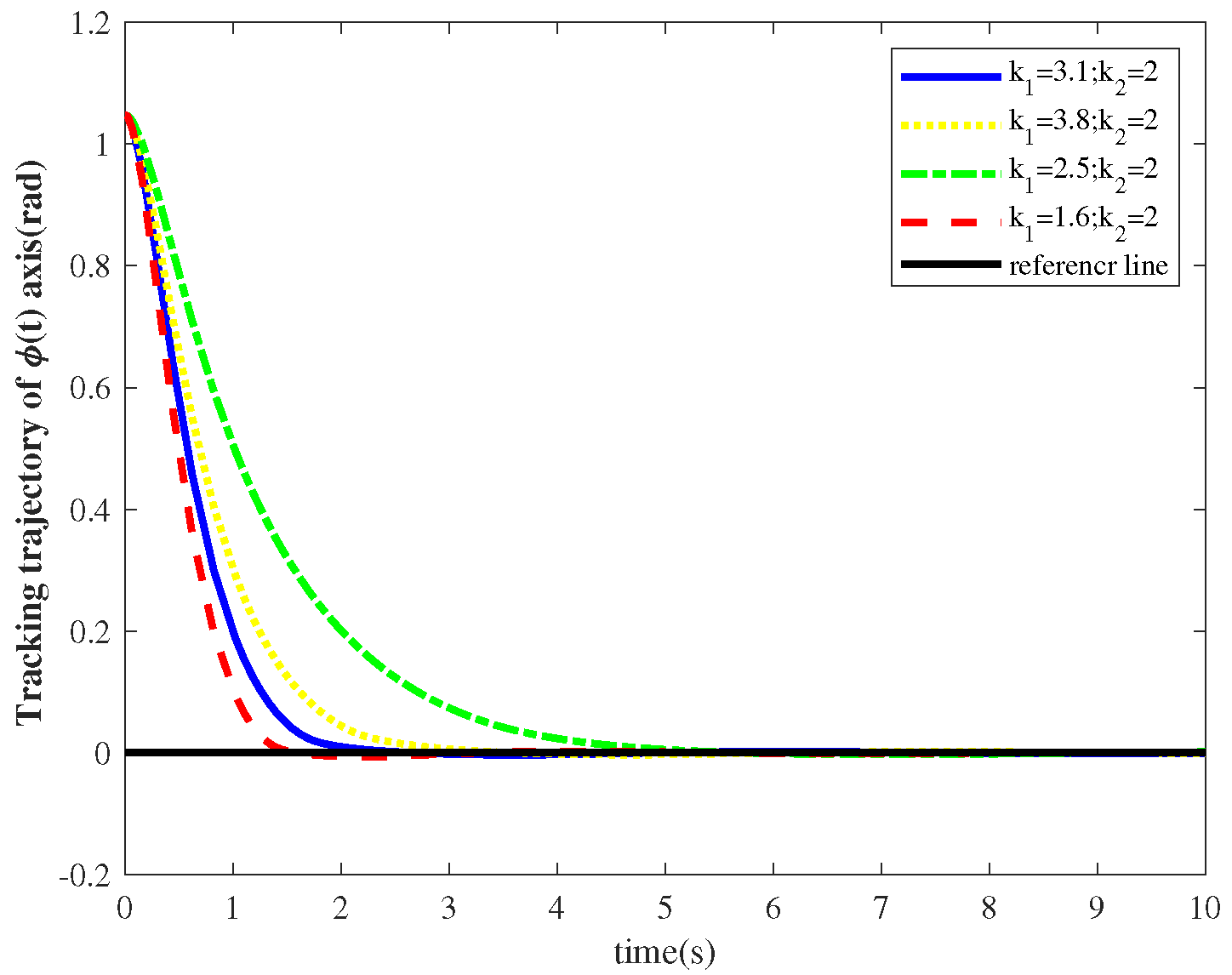
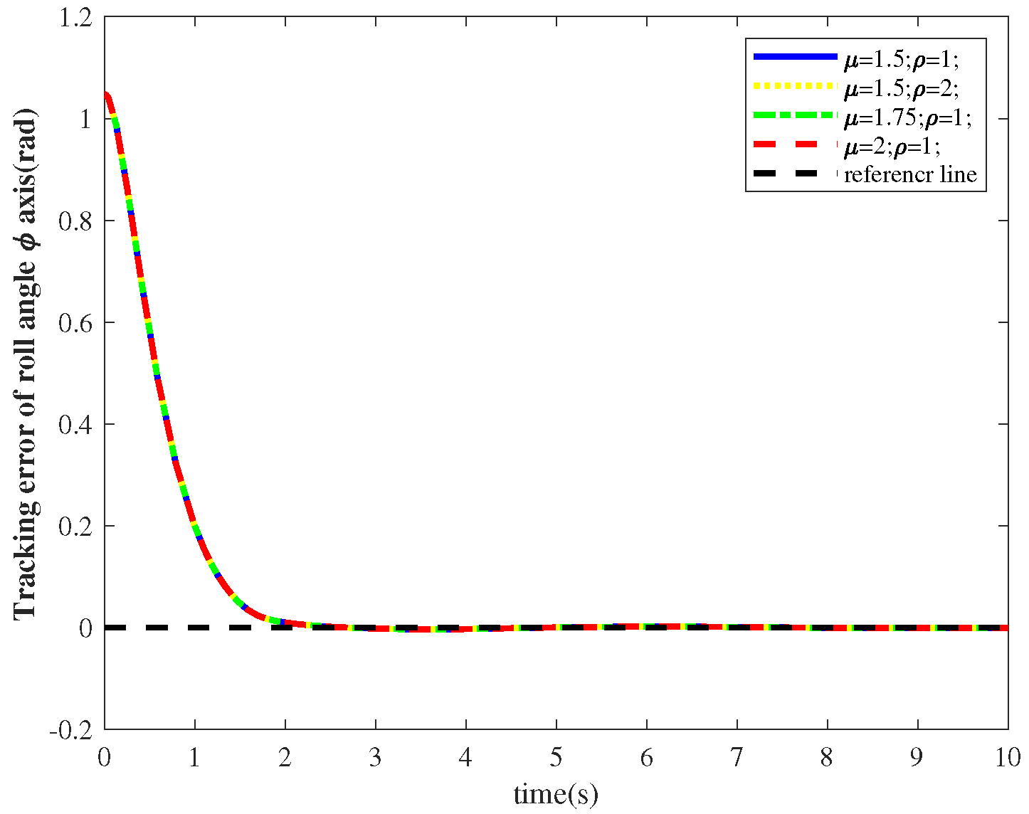
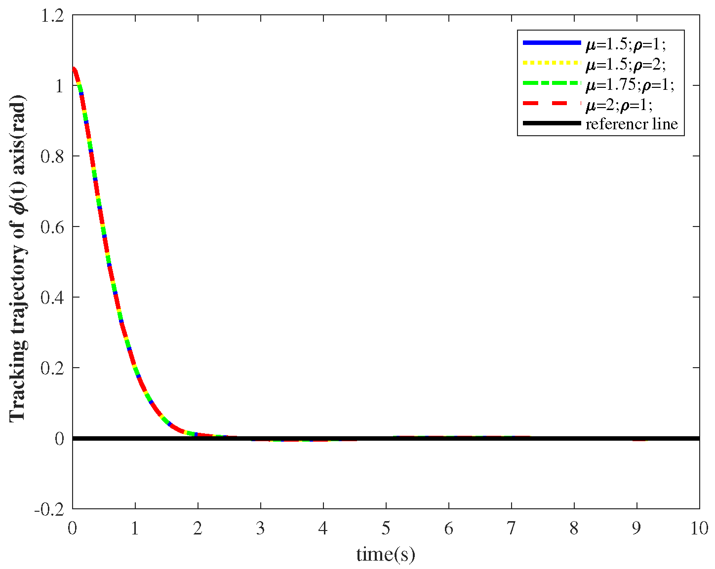
4.1. Attitude Tracking Control under FTISMC

The switching controller proposed in this paper requires the attitude subsystem to control the attitude angles ϕ , θ , and ψ to ϕ d , θ d , and ψ d , respectively, and so the effectiveness of the attitude controller FTISMC is proven first. Four different controllers were used for the simulation experiments, which are FTISMC, non-singular fast terminal sliding mode controller (NFTSMC) [23], finite-time controller (FC) [41], and proportional differential controller (PD). The control parameters used in the experiment are shown in Table 2. Figure 2 shows the simulation results of the attitude angle tracking error under the control of different controllers. In Figure 3 and Figure 4, the attitude angle and angular velocity under the control of different controllers vary with time. From Figure 2, Figure 3 and Figure 4, it can be seen that the attitude subsystem controlled by FTISMC has a faster convergence speed compared to other controllers. Among them, the subsystems controlled by FC and PD converge similarly and more slowly.
Additionally, Figure 5 shows the simulation comparison results of the attitude subsystem control of the inputs designed in this paper. Table 3 clearly shows the performances of different controllers through three performance metrics: stabilization time, maximum overshoot, and peak time. The FTISMC stabilization time is faster, the maximum overshoot is acceptable, and the overall control performance is better, as seen in Figure 5 and Table 3.
Next, the parameter sensitivity of FTISMC is analyzed. The integral gains k 1 and k 2 determine the returned value of the integral element in the sliding mode variable s e 1 in (14). According to (19), the fixed time T r is inversely proportional to k 1 . A larger k 1 can increase the convergence rate of s e 1 , as well as the amplitude of the integral element in (14), but it may also cause severe chattering. Similarly, a smaller k 2 reduces the convergence time but leads to a smaller overshoot. Additionally, the larger parameters ρ and μ will result in larger dithering. Thus, we have to choose the right parameters for the experiment.
Taking the ϕ —subsystem as an example, when FTISMC chooses different parameters k 1 and k 2 , the simulation results of the roll angle control are shown in Figure 6, Figure 7, Figure 8 and Figure 9. When k 1 = 3.8 and k 2 = 2 , although the trajectory converges the fastest, the overshoot is too large. Additionally, when k 1 = 1.6 and k 2 = 2 , although the overshoot is smaller, the convergence speed is the slowest. Therefore, the parameters k 1 = 3.1 and k 2 = 2 are chosen for the comprehensive experimental comparison. As can be seen by Figure 10, Figure 11, Figure 12 and Figure 13, the attitude angle control results do not significantly change with different parameters μ and ρ . Therefore, the controller is not sensitive to the selection of these two parameters.

4.2. Position Tracking Control under a Continuous Fixed-Time Controller

To prove the effectiveness of the continuous fixed-time controller with the constraints proposed in this paper, a comparative test was designed. In the position subsystem, three different controllers were used for the simulation experiments, which are the fixed-time controller proposed in this paper, the finite-time controller [41], and the traditional PD controller. The simulation parameters are shown in Table 4. According to [42], we chose function β n ( x ¯ n ) = 1 + i = 1 n | x i | 2 2 in Appendix A.1, Lemma A1. Figure 14 shows the simulation results of three different controllers in the position subsystem. Then, Figure 15 shows the simulation comparison results of the position subsystem control input. Similarly, Table 5 shows the control performances of different control inputs U 1 according to three metrics: stabilization time, maximum overshoot, and peak time.
In order to verify that the proposed fixed-time controller has fixed-time characteristics, three sets of different initial states were selected for the simulation experiments. These three sets of randomly selected initial conditions are I1: [ x 0 , y 0 , z 0 ] T = [ 3 , 2 , 20 ] T , I2: [ x 0 , y 0 , z 0 ] T = [ 12 , 1 , 6 ] T , and I3: [ x 0 , y 0 , z 0 ] T = [ 5 , 9 , 8 ] T , respectively, and the parameters were selected to remain the same. The position tracking error simulation results are shown in Figure 16. It is obvious that the fixed-time controller can obtain a very fast convergence speed, and the convergence time is basically the same under the three different initial states. According to the simulation results, it is clear that the convergence time of the proposed control method does not depend on the initial value of the system.
In the switching control designed in this paper, through a theoretical analysis, it can be known that the control input of the attitude angle subsystem has only a small change in the switching process, so that the change process from the three attitude angles ϕ , θ to the target attitude angle ϕ T , θ T , and ψ T is a continuous change process. It can be clearly seen from Figure 15 that the control input of the position subsystem changes from U 1 in (23) to U 1 = g after switching.
In addition, the control inputs U 1 , U 2 , U 3 , and U 4 are related to the rotor speeds ω 1 , ω 2 , ω 3 , and ω 4 by Equation (1), which gives:
ω 1 2 ω 2 2 ω 3 2 ω 4 2 = 1 4 1 0 2 1 1 2 0 1 1 0 2 1 1 2 0 1 m b U 1 J x l b U 2 J y l b U 3 J z d U 4 ,
where m , b , l , d , J x , J y , and J z are parameters. The control inputs U 1 , U 2 , U 3 , and U 4 can be obtained by Theorem 3, and the real control rotor speeds ω 1 , ω 2 , ω 3 , and ω 4 can be obtained by Equation (25). In the actual flight control process, the overall control of the QUAV can be completed by controlling the rotor speeds ω 1 , ω 2 , ω 3 , and ω 4 .
In summary, it can be seen from Figure 2 and Figure 14 that the quadrotor can quickly complete the hovering task of six states of the position and attitude under the switching control scheme designed in this paper. Through the simulation image, we can also see that the altitude tracking error of the QUAV is constantly decreasing, thus verifying the conclusion that there will be no crash.

5. Conclusions

In this article, a novel switching mode control law was proposed to control the position and attitude of QUAVs so that their six states can be stabilized at a given particular posture point for a fixed time. For the position subsystem, a continuously differentiable fixed-time controller with a double-integral form was designed, and, for the attitude subsystem, a fixed-time attitude controller was designed; finally, the whole flight switching controller was presented and the crash problem was analyzed in detail by switching the mode control law. In addition, simulations were designed to compare the experiments with existing research methods. The experiments show that the proposed control method can control the error to converge to zero within 3 s. Additionally, the sensitivity of the controller parameters was analyzed through simulation experiments, and it was proven that the switching mode control algorithm improves the control performance without depending on the initial state. The readers can refer to the parameters in Section 4 when reproducing the simulation experiment. However, the system model established in this paper does not take into account the effects of external disturbances and air resistance. In future work, influence factors such as the gyro moment, air resistance, and external interference will be fully considered so that the QUAV can still achieve full state control while remaining under influence.

Author Contributions

Conceptualization, N.C. and C.W.; methodology, N.C. and C.W.; software, N.C.; validation, N.C. and C.W.; formal analysis, N.C.; investigation, N.C. and C.W.; resources, C.W.; writing—original draft preparation, N.C.; writing—review and editing, N.C. and C.W.; supervision, C.W.; project administration, C.W.; funding acquisition, C.W. All authors have read and agreed to the published version of the manuscript.

Funding

This paper was partially supported by the Nature Science Foundation of China under Grant (6217023627, 62003214, 62173054, 6217323), the National Defense Basic Research Program (JCKY2019413D001) and the development plan of military medical research and innovation team.

Data Availability Statement

The data that support the findings of this study are available within the article.

Acknowledgments

The authors thank their schoolmates for their suggestions and research assistance throughout the study.

Conflicts of Interest

The authors declare no conflict of interest.

Appendix A

Appendix A.1. Some Relevant and Important Lemmas

 Lemma A1
([42]). Consider the following system:
x ˙ i ( t ) = x i + 1 ( t ) , i = 1 , 2 , , n 1 x ˙ n ( t ) = u ( t )
with the initial condition x ( 0 ) = x 0 , where x ( t ) = ( x 1 , , x n ) T R n and u ( t ) R are the system state and input, respectively. Define a set of continuous virtual controllers x 1 * , , x n * , shown as:
x 1 * = 0 , ζ 1 = x 1 1 r 1 x 1 * 1 r 1 , x i * = β i 1 ( x ¯ i 1 ) ζ i 1 r i , ζ i = x i 1 r i x i * 1 r i , ( i = 1 , 2 , , n )
with constants v ( 1 n , 0 ) and r i = 1 + ( i 1 ) v , and continuous scalar functions β j ( x ¯ j ) > 0 , j = 1 , , i 1 , where x ¯ j Γ j σ :
Γ j σ = { x ¯ j ( t ) : x ¯ j ( t ) R j , | x 1 ( t ) | < σ } , j = 1 , , i 1 .
If the controller u ( t ) of system (A1) is designed as:
u ( t ) = β n ( x ¯ n ) ζ n r n + 1
with design parameters l 1 > 0 , l 2 > 0 and v < p < 2 2 v , satisfying:
2 ( v 2 ) l 1 v + ( 2 v ) 2 2 + p 2 v n p + v 2 v l 2 ( p + v ) < T ,
then, for all x 1 ( 0 ) Ω , where Ω = { w | w R , | w | < σ } is a constraint and σ is a positive constant, the following properties are established.
(i) The state x 1 ( t ) stays in the set Ω for all t 0 .
(ii) All states of the whole closed-loop system can be adjusted to zero within a fixed time T.
 Remark A1.
This is the result of the fixed-time stabilization design of multiple series integrators, where the time T is independent of the initial value of the system.
 Lemma A2
([43]). Consider the system (A1), and x 0 R n represents the initial condition of the system. If the controller is designed as:
u ( t ) = i = 1 n k i ( x i ϱ i + x i + x i ϱ i ) .
where the parameters ϱ i , ϱ i , ( i = 1 , 2 , , n ) are calculated by:
ϱ n j = ϱ ( j + 1 ) j ϱ , ϱ n j = 2 ϱ j ϱ ( j 1 ) , ( j = 0 , 1 , , n 1 ) .
If ϱ ( ϵ , 1 ) and the parameters k i > 0 , ( i = 1 , 2 , , n ) are chosen to ensure that the n-order polynomials s n + k n s n 1 + + k 1 and s n + 3 k n s n 1 + + 3 k 1 are Hurwitz, then there exists a positive real number ϵ in the interval ( 1 2 , 1 ) such that the origin of system (A1) is fixed-time stable for any initial condition x 0 R n .
 Remark A2.
Compared with Lemma A1, the fixed-time control law designed by Lemma A2 has no constraints and is more general.
 Lemma A3
([11,44]). Consider the following system:
x ˙ ( t ) = f ( t , x ) , x ( 0 ) = x 0 ,
where x R n and f : R + × R n R n is a nonlinear function.
If there exists a continuous radially unbounded and positive definite function V ( x ) such that
V ˙ ( x ) α V p β V q
for some α , β > 0 , p > 1 , 0 < q < 1 , then the origin of this system (A5) is globally fixed-time stable and the settling time function T can be estimated by:
T T m a x : = 1 α ( p 1 ) + 1 β ( 1 q ) .
In addition, if p = 1 + 1 μ and q = 1 1 μ with μ > 1 are selected, the settling time function T can be estimated using a less conservative bound:
T m a x : = π μ 2 α β .

Appendix A.2. The Properties of the Arctangent Function

In the following, an angle calculation function often encountered in the robotics textbook [45], namely, the arctangent function, abbreviated a t a n 2 , is defined as follows:
a t a n 2 ( a , b ) = a r c t a n ( a b ) , b > 0 a r c t a n ( a b ) + π , a 0 , b < 0 a r c t a n ( a b ) π , a < 0 , b < 0 π 2 , a > 0 , b = 0 π 2 , a < 0 , b = 0 u n d e f i n e d . a = 0 , b = 0
This function establishes the one-to-one correspondence between the plane points and angles in the complex plane. This function has the following characteristics.
 Property A1.
Consider the following inverse function z = a t a n 2 ( a , b ) , where z π , π , and a and b represent the constant values of the x-axis coordinates and y-axis coordinates, respectively. The following two conclusions hold.
(1) If the constant c > 0 is chosen, then there is:
z = a t a n 2 ( a c , b c ) = a t a n 2 ( a , b ) ,
(2) If the constant c < 0 is chosen, then there is:
z = a t a n 2 ( a c , b c ) = a t a n 2 ( a , b ) π , a > 0 , b > 0 a t a n 2 ( a , b ) + π , a 0 , b > 0 a t a n 2 ( a , b ) , b < 0 π 2 , a > 0 , b = 0 π 2 , a < 0 , b = 0 u n d e f i n e d . a = 0 , b
 Remark A3.
After analyzing the situation when the non-zero constant c takes different values, it is easy to obtain Property A1 based on the property of inverse function 2.

Appendix A.3. The Proof of Theorem 1

It can be seen from (16), (19), and (20) that the structures of the three subsystems controlled by a ( t ) , b ( t ) , and c ( t ) are the same. We only need to prove one. Taking the z-axis direction as an example, the stability analysis of the system is as follows.
At first, the z-error subsystem is transformed by defining z 1 z ( t ) = e 11 ( t ) , z 2 z ( t ) = e 12 ( t ) , z 3 z ( t ) = c ( t ) , z 4 z ( t ) = c ˙ ( t ) , z ˙ 4 z ( t ) = u ( t ) , and then the fourth-order integrator system is given:
z ˙ 1 z ( t ) = z 2 z ( t ) , z ˙ 2 z ( t ) = z 3 z ( t ) , z ˙ 3 z ( t ) = z 4 z ( t ) , z ˙ 4 z ( t ) = u ( t ) .
Define a set of continuous virtual controllers z 1 z * ( t ) , , z 4 z * ( t ) , shown as:
z 1 z * ( t ) = 0 , ζ 1 z ( t ) = z 1 z ( t ) 1 r 1 z z 1 z * ( t ) 1 r 1 z , z i z * ( t ) = β i 1 ( z ¯ ( i 1 ) z ) ζ i 1 ( t ) r i z , ζ i z ( t ) = z i z ( t ) 1 r i z z i z * ( t ) 1 r i z , ( i = 1 , 2 , 3 , 4 )
with constants v ( 1 n , 0 ) , r i z = 1 + ( i 1 ) v for i = 1 , , 4 , and smooth functions β j ( z ¯ j z ) > 0 for j = 1 , , 4 , where there is z ¯ j z Γ j z σ z :
Γ j z σ z = { z ¯ j z ( t ) : z ¯ j z ( t ) R j , | z j z ( t ) | < σ z } .
For all z j z ( 0 ) Γ 4 z σ z , if the controller u of system (A11) is designed as:
u ( t ) = z 5 z * ( t ) = β 4 ( z ¯ 4 z ) ζ 4 z ( t ) r 5 z
with design parameters l 1 > 0 , l 2 > 0 and v < p < 2 2 v satisfying:
2 ( v 2 ) l 1 v + ( 2 v ) 2 2 + p 2 v n p + v 2 v l 2 ( p + v ) < T z ,
it follows from Lemma A1 that the closed loop system composed of (6), (9), and (10) is stable for a fixed time.
According to (10), u ( 0 ) = 0 and u ˙ ( 0 ) = 0 . Integrating the controller u ( t ) with a double gives z 3 z ( t ) = c ( t ) , as shown in Equation (10). Therefore, the second-order system (6) is also fixed-time stable when using the controller c ( t ) , i.e., there exists a constant T z that is independent of the initial conditions, such that e 11 ( t ) 0 , e 12 ( t ) 0 and e 11 ( t ) Ω e 11 for all t T z .
Similar to the above proof, it can be proven that the proposed controllers also guarantee the QUAV to track its desired trajectory in the x and y position channels.
The proof is completed.

Appendix A.4. The Proof of Proposition 1

Because ϕ d = 0 , it is only necessary to check:
a c o s ψ d + b s i n ψ d = U 1 s i n θ d
a s i n ψ b c o s ψ = 0
c + g = U 1 c o s θ d
From Equation (12), it is clear that
s i n θ d = a 2 + b 2 U 1 , c o s θ d = c + g U 1 , s i n ψ d = b a 2 + b 2 , c o s ψ d = a a 2 + b 2 .
Therefore, there are:
a c o s ψ d + b s i n ψ d = a 2 a 2 + b 2 + b 2 a 2 + b 2 = a 2 + b 2 = U 1 · a 2 + b 2 U 1 = U 1 s i n θ d .
Thus, (A15a) is established.
In addition,
a s i n ψ d b c o s ψ d = a b a 2 + b 2 a b a 2 + b 2 = 0 .
Therefore, (A15b) is established.
Then, consider:
U 1 c o s θ d = U 1 · c + g U 1 = c + g .
Thus, (A15c) is established, so Equation (11) holds.
The proof is completed.

References

  1. Deepak, B.B.V.L.; Singh, P. A survey on design and development of an unmanned aerial vehicle (quadcopter). Int. J. Intell. Unmanned Syst. 2016, 4, 70–106. [Google Scholar]
  2. Bai, Y.Q.; Liu, H.; Shi, Z.Y.; Zhong, Y. Robust flight control of quadrotor unmanned air vehicles. Jiqiren (Robot) 2012, 34, 519–524. [Google Scholar] [CrossRef]
  3. Ma, F.Y.; Yang, Z.; Ji, P. Sliding mode controller based on the extended state observer for plant-protection quadrotor unmanned aerial vehicles. Mathematics 2022, 10, 1346. [Google Scholar] [CrossRef]
  4. Wang, F.; Xian, B.; Huang, G.P.; Zhao, B. Autonomous hovering control for a quadrotor unmanned aerial vehicle. In Proceedings of the 32nd Chinese Control Conference (CCC), Xi’an, China, 26–28 July 2013; pp. 620–625. [Google Scholar]
  5. Basri, M.A.M. Robust Backstepping controller design with a fuzzy compensator for autonomous hovering quadrotor UAV. Iran. J. Sci. Technol. Trans. Electr. Eng. 2018, 42, 379–391. [Google Scholar] [CrossRef]
  6. Zhou, L.H.; Zhang, B. Quadrotor UAV flight control using backstepping adaptive controller. In Proceedings of the IEEE 6th International Conference on Control Science and Systems Engineering (ICCSSE), Beijing, China, 17–19 July 2020; pp. 169–172. [Google Scholar]
  7. Wang, M.; Chen, B.; Lin, C. Prescribed finite-time adaptive neural trajectory tracking control of quadrotor via output feedback. Neurocomputing 2021, 458, 364–375. [Google Scholar] [CrossRef]
  8. Rao, J.J.; Li, B.; Zhang, Z. Position control of quadrotor UAV based on cascade fuzzy neural network. Energies 2022, 15, 1763. [Google Scholar] [CrossRef]
  9. Wang, F.; Ma, Z.G.; Gao, H.M. Disturbance observer-based nonsingular fast terminal sliding mode fault tolerant control of a quadrotor UAV with external disturbances and actuator faults. Int. J. Control Autom. Syst. 2022, 20, 1122–1130. [Google Scholar] [CrossRef]
  10. Li, S.; Sun, Z.; Talpur, M.A. A finite time composite control method for quadrotor UAV with wind disturbance rejection. Comput. Electr. Eng. 2022, 103, 108299. [Google Scholar] [CrossRef]
  11. Polyakov, A. Nonlinear feedback design for fixed-time stabilization of linear control systems. IEEE Trans. Autom. Control 2012, 57, 2106–2110. [Google Scholar] [CrossRef] [Green Version]
  12. Zhou, S.C.; Guo, K.X.; Yu, X. Fixed-time observer based safety control for a quadrotor UAV. IEEE Trans. Aerosp. Electron. Syst. 2021, 57, 2815–2825. [Google Scholar] [CrossRef]
  13. Liu, K.; Wang, R.J.; Zheng, S.J. Fixed-time disturbance observer-based robust fault-tolerant tracking control for uncertain quadrotor UAV subject to input delay. Nonlinear Dyn. 2022, 107, 2363–2390. [Google Scholar] [CrossRef]
  14. Guo, K.X.; Zhang, W.Y.; Zhu, Y.K. Safety control or quadrotor UAV against ground effect and blade damage. IEEE Trans. Ind. Electron. 2022, 69, 13373–13383. [Google Scholar] [CrossRef]
  15. Liu, L.; Liu, J.J.; Li, J.F. Fault-tolerant control for quadrotor based on fixed-time ESO. Mathematics 2022, 10, 4386. [Google Scholar] [CrossRef]
  16. Ma, D.; Xia, Y.; Shen, G. Practical fixed-time disturbance rejection control for quadrotor attitude tracking. IEEE Trans. Ind. Electron. 2021, 68, 7274–7283. [Google Scholar] [CrossRef]
  17. Shao, X.L.; Tian, B.; Yang, W. Fixed-time trajectory following for quadrotors via output feedback. ISA Trans. 2021, 68, 213–224. [Google Scholar] [CrossRef]
  18. Li, X.; Qi, G.Y.; Zhang, L.M. Time-varying formation dynamics modeling and constrained trajectory optimization of multi-quadrotor UAVs. Nonlinear Dyn. 2021, 106, 3265–3284. [Google Scholar] [CrossRef]
  19. Li, B.; Gong, W.Q.; Yang, Y.S. Appointed fixed time observer-based sliding mode control for a quadrotor UAV under external disturbances. IEEE Trans. Aerosp. Electron. Syst. 2022, 58, 290–303. [Google Scholar] [CrossRef]
  20. Ai, X.L.; Yu, J.Q. Fixed-time trajectory tracking for a quadrotor with external disturbances: A flatness-based sliding mode control approach. Aerosp. Sci. Technol. 2019, 89, 58–76. [Google Scholar] [CrossRef]
  21. Mechali, O.; Xu, L.; Huang, Y. Observer-based fixed-time continuous nonsingular terminal sliding mode control of quadrotor aircraft under uncertainties and disturbances for robust trajectory tracking: Theory and experiment. Control Eng. Pract. 2021, 111, 104806. [Google Scholar] [CrossRef]
  22. Gong, W.Q.; Li, B.; Yang, Y.S. Fixed-time integral-type sliding mode control for the quadrotor UAV attitude stabilization under actuator failures. Aerosp. Sci. Technol. 2019, 95, 105444. [Google Scholar] [CrossRef]
  23. Hua, C.C.; Wang, K.; Chen, J.N. Tracking differentiator and extended state observer-based nonsingular fast terminal sliding mode attitude control for a quadrotor. Nonlinear Dyn. 2018, 94, 343–354. [Google Scholar] [CrossRef]
  24. Yang, S.; Han, J.; Xia, L. Adaptive robust servo constraint tracking control for an underactuated quadrotor UAV with mismatched uncertainties. ISA Trans. 2020, 106, 12–30. [Google Scholar] [CrossRef] [PubMed]
  25. Tripathi, V.K.; Kamath, A.K.; Behera, L. Finite-time super twisting sliding mode controller based on higher-order sliding mode observer for real-time trajectory tracking of a quadrotor. IET Control Theory Appl. 2020, 14, 2359–2371. [Google Scholar] [CrossRef]
  26. Moeini, A.; Lynch, A.F.; Zhao, Q. A backstepping disturbance observer control for multirotor UAVs: Theory and experiment. Int. J. Control 2022, 95, 2364–2378. [Google Scholar] [CrossRef]
  27. Mu, C.; Zhang, Y. Learning-based robust tracking control of quadrotor with time-varying and coupling uncertainties. IEEE Trans. Neural Netw. Learn. Syst. 2020, 31, 259–273. [Google Scholar] [CrossRef] [PubMed]
  28. Miranda-Colorado, R.; Aguilar, L.T.; Herrero-Brito, J.E. Reduction of power consumption on quadrotor vehicles via trajectory design and a controller-gains tuning stage. Aerosp. Sci. Technol. 2018, 78, 280–296. [Google Scholar] [CrossRef]
  29. Miranda-Colorado, R.; Aguilar, L.T. Robust PID control of quadrotors with power reduction analysis. ISA Trans. 2020, 98, 47–62. [Google Scholar] [CrossRef]
  30. Choi, Y.C.; Ahn, H.S. Nonlinear control of quadrotor for point tracking: Actual implementation and experimental tests. IEEE/ASME Trans. Mechatron. 2015, 20, 1179–1192. [Google Scholar] [CrossRef]
  31. Zhu, W.; Du, H.; Cheng, Y. Hovering control for quadrotor aircraft based on finite-time control algorithm. Nonlinear Dyn. 2017, 88, 2359–2369. [Google Scholar] [CrossRef]
  32. Shao, S.; Wang, S.; Zhao, Y. Fixed time output feedback control for quadrotor unmanned aerial vehicle under disturbances. Proc. Inst. Mech. Eng. Part G J. Aerosp. Eng. 2022, 236, 3554–3566. [Google Scholar] [CrossRef]
  33. Huang, T.; Huang, D.; Wang, Z. Robust tracking control of a quadrotor UAV based on adaptive sliding mode controller. Omplexity 2019, 2019, 7931632. [Google Scholar] [CrossRef]
  34. Xu, L.X.; Ma, H.J.; Guo, D. Backstepping sliding-mode and cascade active disturbance rejection control for a quadrotor UAV. IEEE Trans. Mechatron. 2020, 25, 2743–2753. [Google Scholar] [CrossRef]
  35. Labbadi, M.; Cherkaoui, M. Robust adaptive nonsingular fast terminal sliding-mode tracking control for an uncertain quadrotor UAV subjected to disturbances. ISA Trans. 2020, 99, 290–304. [Google Scholar] [CrossRef] [PubMed]
  36. Lee, K.U.; Kim, H.S.; Park, J.B. Hovering control of a quadrotor. In Proceedings of the 12th International Conference on Control, Automation and Systems (ICCAS), Jeju, Republic of Korea, 17–21 October 2012; pp. 162–167. [Google Scholar]
  37. Majd, S.; THassan, S.; Benjamin, L. Local controllability and attitude stabilization of multirotor UAVs: Validation on a coaxial octorotor. Rob. Auton. Syst. 2017, 91, 128–138. [Google Scholar]
  38. Wang, F.; Gao, H.; Wang, K. Disturbance observer-based finite-time control design for a quadrotor UAV with external disturbance. IEEE Trans. Aeros. Elect. Syst. 2021, 57, 834–847. [Google Scholar] [CrossRef]
  39. Filippov, A.F. Differential Equations with Discontinuous Righthand Sides: Control Systems; Kluwer: Dordrecht, The Netherlands, 1988. [Google Scholar]
  40. Suleiman, H.U.; Mu’azu, M.B.; Arma, T.A. Methods of chattering reduction in sliding mode control: A case study of ball and plate system. In Proceedings of the 2018 IEEE 7th International Conference on Adaptive Science and Technology (ICAST), Accra, Ghana, 22–24 August 2018; pp. 1–8. [Google Scholar]
  41. Wu, D.; Zhang, W.; Du, H. Robust adaptive finite-time trajectory tracking control of a quadrotor aircraft. Int. J. Robust Nonlinear Control 2021, 31, 8030–8054. [Google Scholar] [CrossRef]
  42. Yao, H.; Gao, F.; Huang, J. Barrier lyapunov functions-based fixed-time stabilization of nonholonomic systems with unmatched uncertainties and time-varying output constraints. Nonlinear Dyn. 2020, 99, 2835–2849. [Google Scholar] [CrossRef]
  43. Tian, B.; Lu, H.; Zuo, Z. Fixed-time stabilization of high-order integrator systems with mismatched disturbance. Nonlinear Dyn. 2018, 94, 2889–2899. [Google Scholar] [CrossRef]
  44. Parsegov, S.E.; Polyakov, A.E.; Shcherbakov, P.S. Fixed-time consensus algorithm for multi-agent systems with integrator dynamics. IFAC Proc. Vol. 2013, 46, 110–115. [Google Scholar] [CrossRef] [Green Version]
  45. Craig, J.J. Introduction to Robotics: Mechanics and Control, 4th ed.; Pearson: New York, NY, USA, 2018; pp. 109–145. [Google Scholar]
Figure 1. The theoretical model of QUAV.
Mathematics 11 00994 g001
Figure 2. Attitude angle tracking error of different controllers.
Mathematics 11 00994 g002
Figure 3. Attitude angle tracking trajectories of different controllers.
Mathematics 11 00994 g003
Figure 4. Attitude angle tracking trajectories of different controllers.
Mathematics 11 00994 g004
Figure 5. Control inputs of different controllers.
Mathematics 11 00994 g005
Figure 6. ϕ of different k 1 and k 2 .
Mathematics 11 00994 g006
Figure 7. ϕ ˙ of different k 1 and k 2 .
Mathematics 11 00994 g007
Figure 8. e ϕ of different k 1 and k 2 .
Mathematics 11 00994 g008
Figure 9. U 2 of different k 1 and k 2 .
Mathematics 11 00994 g009
Figure 10. ϕ of different μ and ρ .
Mathematics 11 00994 g010
Figure 11. ϕ ˙ of different μ and ρ .
Mathematics 11 00994 g011
Figure 12. e ϕ of different μ and ρ .
Mathematics 11 00994 g012
Figure 13. U 2 of different μ and ρ .
Mathematics 11 00994 g013
Figure 14. Position tracking errors of different controllers.
Mathematics 11 00994 g014
Figure 15. Control input U 1 of different controllers.
Mathematics 11 00994 g015
Figure 16. Position tracking error of different initial values.
Mathematics 11 00994 g016
Table 1. Parameters of QUAV dynamics.
ParameterMeaning
x y z T Coordinates in the inertial frame
ϕ θ ψ T Roll, pitch, and yaw angles
J x J y J z T Inertial moments, along with given directions
ω 1 ω 2 ω 3 ω 4 T Angular velocities of the four rotors
U 1 U 2 U 3 U 4 T Thrust and torques, along with given directions
m g T Mass and gravitational acceleration
b d l T Lift coefficient, antitorque coefficient, and length of the quadrotor arm
Table 2. The control parameters in the experiments.
ControllerControl Parameters
FTISMC k 1 = k 3 = k 5 = 3.1 , k 2 = k 4 = k 6 = 2 , ϱ 1 = ϱ 3 = ϱ 5 = 0.6 , ϱ 1 = ϱ 3 = ϱ 5 = 1.667 , ϱ 2 = ϱ 4 = ϱ 6 = 0.75 , ϱ 2 = ϱ 4 = ϱ 6 = 1.25 , μ = 1.5 , ρ = 1 , δ = 0.05
NFTSMC k 1 = k 2 = k 5 = k 6 = k 9 = k 10 = 0.5 , k 3 = k 7 = k 11 = 0.8 , k 4 = k 8 = k 12 = 1 , λ 1 = λ 3 = λ 5 = 7 , λ 2 = λ 4 = λ 6 = 5 , q 1 = q 2 = q 3 = 5 , p 1 = p 2 = p 3 = 3
FC a p 1 = a p 2 = a p 3 = 4.5 , a d 1 = a d 2 = a d 3 = 5.5 , b 1 = b 3 = b 5 = 0.75 , b 2 = b 4 = b 6 = 0.857
PD k p 1 = k p 2 = k p 3 = 3 , k d 1 = k d 2 = k d 3 = 4
Table 3. Summary and comparison of attitude subsystem controllers performances.
Attitude ControllerSettling Time(s)Maximum OvershootPeak Time(s)
Schemes U 2 U 3 U 4 U 2 U 3 U 4 U 2 U 3 U 4
FTISMC2.1742.2882.2832.6470.39610.93060.5061.4470.6305
NFTSMC2.2882.7543.5311.6720.9591.0720.71741.4031.15
FC4.143.743.6520.7520.0790.3130.6022.0621.054
PD4.143.943.8290.710.0740.2930.7912.0621.174
Table 4. The control parameters in the experiments.
ControllerControl Parameters
fixed-time controller σ = 10 , v = 0.2 , p = 2 , l = 3
finite-time controller k p 1 = k p 2 = k p 3 = 4.5 , k d 1 = k d 2 = k d 3 = 5.5 , a 1 = a 3 = a 5 = 0.75 , a 2 = a 4 = a 6 = 0.857
traditional controller k p 1 = k p 2 = k p 3 = 3 , k d 1 = k d 2 = k d 3 = 4
Table 5. Summary and comparison of attitude subsystem controllers performances.
Position Controller U 1 Settling Time(s)Maximum OvershootPeak Time(s)
fixed-time controller3.0225.430.046
finite-time controller4.8360.230.184
traditional controller3.6543.060.498
Disclaimer/Publisher’s Note: The statements, opinions and data contained in all publications are solely those of the individual author(s) and contributor(s) and not of MDPI and/or the editor(s). MDPI and/or the editor(s) disclaim responsibility for any injury to people or property resulting from any ideas, methods, instructions or products referred to in the content.

