M-Polar Fuzzy Graphs and Deep Learning for the Design of Analog Amplifiers

Abstract

The design of analog circuits is a complex and repetitive process aimed at finding the best design variant. It is characterized by uncertainty and multivariate approaches. The designer has to make different choices to satisfy a predefined specification with required parameters. This paper proposes a method for facilitating the design of analog amplifiers based on m-polar fuzzy graphs theory and deep learning. M-polar fuzzy graphs are used because of their flexibility and the possibility to model different real-life multi-attribute problems. Deep learning is applied to solve a regression task and to predict the membership functions of the m-polar fuzzy graph vertices (the solutions), taking on the role of domain experts. The performance of the learner is high since the obtained errors are very small: Root Mean Squared Error is from 0.0032 to 0.0187, Absolute Error is from 0.022 to 0.098 and Relative Error is between 0.27% and 1.57%. The proposed method is verified through the design of three amplifiers: summing amplifier, subtracting amplifier, and summing/subtracting amplifier. The method can be used for improving the design process of electronic circuits with the possibility of automating some tasks.

1. Introduction

The design process of analog circuits is characterized by its complexity and uncertainty, but also by its multivariate approaches. According to one predefined specification with initial parameters, it is possible to have multiple solutions that satisfy this assignment. It is obvious that the designer must find the best design by entering one iterative procedure, and making one or another decision. In support of the designer, a wide variety of methods and methodologies are proposed—from the use of standard matrix theory [1] to contemporary machine learning approaches [2].

The topic related to machine learning-driven design of analog circuits is under extensive investigation, because of the desire for facilitating the designer and automating as many engineering tasks as possible. This could reduce the design time, increase the design quality and decrease the effort of both a beginner and experienced engineer.

Some works show the applicability of evolutionary computing in analog circuit design and possibilities for time controlling [3], achieving efficient and flexible design [4], and design optimization [5]. Bayesian optimization techniques are also under investigation, pointing out another different possible approach for improving the circuit design process regarding design speed and accuracy [6,7].

Deep learning (DL) as a part of machine learning is based on architectures of artificial neural networks (ANNs) and is used for solving classification or regression tasks in different domains and industries, including electronic circuit design [8] and analysis [9]. This popularity of supervised DL is due to its capability to perform predictions and classifications with high accuracy. This is possible because of the flexibility of ANNs construction and DL algorithm parameters adjustment.

Nowadays, the theory of fuzzy graphs gets its popularity due to its wide applications in many areas of real life. The concept of a fuzzy graph was initially introduced by Kauffman [10], but the development of the fuzzy graphs theory is due to Rosenfeld [11] and Yeh and Bang [12]. The fuzzy graphs theory has been developing in different directions, such as fuzzy tolerance graphs [13], fuzzy threshold graphs [14], interval-valued fuzzy graphs [15,16,17], fuzzy k-competition graphs and p-competition fuzzy graphs [18], m−step fuzzy competition graphs [19], and hesitant fuzzy graphs [20]. In 1994, Zhang [21,22] introduced the concept of bipolar fuzzy sets as a generalization of fuzzy sets. This theory was developed by Akram [23] to present bipolar fuzzy graphs. In 2014, Chen et al. [24] discussed the notion of m-polar fuzzy sets as a generalization of bipolar fuzzy sets. Ghorai and Pal [25] introduced the m-polar fuzzy graphs as a generalization of bipolar fuzzy graphs and defined different operations. The theory of m-polar fuzzy graphs was further developed in [26,27,28,29]. A detailed explanation could be found in two contemporary monographs [30,31].

This work is the first to use m-polar fuzzy graphs theory with the benefits of deep learning for the design of analog amplifiers, but we consider the idea to combine the advantages of fuzzy graphs and deep learning to be very promising. Graphs theory is used, taking into account its powerful capability for solving different real-life problems. Modelling of such problems often involves multi-polar information, including uncertainty and process limits, so attracting m-polar fuzzy graphs for describing such problems is very useful. Deep learning predictions are utilized in the role of the domain experts to point out the membership functions of m-polar fuzzy graph vertices. The regression task is solved with high performance.

The aim of the paper is to present a method for designing analog amplifiers by discussing some basic concepts regarding m-polar fuzzy graphs and considering the advantages of deep learning. The following is a summary of the research work’s main contribution:

1. The activity for designing analog amplifiers is defined as a multi-attribute problem, which is solved here using the m-polar fuzzy graphs and deep learning.

2. For the verification of the proposed method, three electronic circuits are designed: an inverting summing amplifier, a subtracting amplifier (differential amplifier), and a summing/subtracting amplifier with an operational amplifier.

3. The predictive models are experimentally evaluated using data sets collected considering the functional and electrical behavior of the examined circuits.

The paper is organized as follows: In Section 2, a review of the basic concept of fuzzy graphs theory and m-polar fuzzy graphs as well as different types of product operations for m-polar fuzzy graphs are presented. Section 3 is dedicated to discussing the usage of ANNs in solving circuit design problems. Section 4 considers the proposed method. In Section 5, the presented method for analog circuit design is demonstrated and verified in the real-life application of analog amplifier design. The conclusion is driven in the last section.

2. Fuzzy Graphs Theory

2.1. Basic Concepts of Fuzzy Graphs

A graph is a pair $G=\left(V, E\right)$ of a nonempty set of vertices $V$ (or nodes) and a set of edges $E$. Each edge has either one or two vertices associated with it, called its endpoints. An edge is said to connect its endpoints. A graph is called simple if it has no loops and no multiple edges.

Definition 1

[32]. A fuzzy graph $G=\left(V,\sigma ,\mu \right)$ is a triple consisting of a nonempty set $V$ together with a pair of functions $\sigma :V\to \left[0,1\right]$ and $\mu :E\to \left[0.1\right]$ such that for all  $x, y\in V$, $\mu \left(xy\right)\le \sigma \left(x\right)\wedge \sigma \left(y\right)$, where $\wedge$ stands for the minimum.

Definition 2

[33]. A fuzzy graph  $G=\left(V,\sigma ,\mu \right)$ is complete if $\mu \left(xy\right)=\sigma \left(x\right)\wedge \sigma \left(y\right)$ for all $x, y\in V$.

Definition 3

[24]. An m-polar fuzzy set (or a ${\left[0,1\right]}^m$ -set) on  $X$ is mapping $M:X\to {\left[0,1\right]}^m$.

The ${\left[0,1\right]}^m$ (m-power of $\left[0,1\right]$) is considered to be a poset with point-wise order $\le$ (m is natural), where $\le$ is defined by $x\le y\iff P_i\left(x\right)\le P_i\left(y\right)$ for each $i=1,2,\dots ,m$, $x,y\in {\left[0,1\right]}^m$, and $P_i:{\left[0,1\right]}^m\to \left[0,1\right]$ is the i−th projection mapping ($i=1,2,\dots ,m$). Here, $1=\left(1, 1,..., 1\right)$ is the greatest value and $0=\left(0, 0,..., 0\right)$ is the smallest value in ${\left[0,1\right]}^m$.

Definition 4

[24]. Let $\sigma$ be an m-polar fuzzy set on a set $V$. An m-polar fuzzy relation on $\sigma$ is an m-polar fuzzy set $\mu$ of $V\times V$ such that $\mu \left(xy\right)\le \sigma \left(x\right)\wedge \sigma \left(y\right)$ for all $x,y\in V$, i.e., for each $i=1,2,\dots ,m$, for all $x,y\in V$: $P_i\circ \mu \left(xy\right)\le P_i\circ \sigma \left(x\right)\wedge P_i\circ \sigma \left(y\right)$.

Definition 5

[30]. An m-polar fuzzy graph $G=\left(V,\sigma ,\mu \right)$ is a triple consisting of a nonempty set $V$ together with a pair of functions $\sigma :V\to {\left[0,1\right]}^m$ and $\mu :E=V\times V$ →${\left[0,1\right]}^m$, where $\sigma$ is an m-polar fuzzy set on the set of vertices $V$ and $\mu$ is an m-polar fuzzy relation in $V$ such that for all $x,y\in V$, $\mu \left(xy\right)\le \sigma \left(x\right)\wedge \sigma \left(y\right)$, where $\wedge$ stands for minimum.

It can be noted that $\mu \left(x,y\right)=0$ for all $x,y\in V\times V-E$.

2.2. Products in m-Polar Fuzzy Graphs

2.2.1. Direct (Tensor) Product

Definition 6

[30]. Let $G_1=\left({\sigma }_1,{\mu }_1\right)$ of $G_1^{*}=\left(V_1,E_1\right)$ and $G_2=\left({\sigma }_2,{\mu }_2\right)$ of $G_2^{*}=\left(V_2,E_2\right)$ be two m-polar fuzzy graphs. The direct product of $G_1$ and $G_2$ is denoted by $G_1\times G_2$ and is defined as a pair $G_1\times G_2=\left({\sigma }_1\times {\sigma }_2,{\mu }_1\times {\mu }_2\right)$, such that for each $i=1,2,\dots ,m$:

$$P_i\circ \left({\sigma }_1\wedge {\sigma }_2\right)\left(x_1,x_2\right)=P_i\circ {\sigma }_1\left(x_1\right)\wedge P_i\circ {\sigma }_2\left(x_2\right) \mathrm{for} \mathrm{all} \left(x_1,x_2\right)\in V_1\times V_2$$

$$P_i\circ \left({\mu }_1\wedge {\mu }_2\right)\left(\left(x_1,x_2\right)\left(y_1,y_2\right)\right)=P_i\circ {\mu }_1\left(x_1{y}_1\right)\wedge P_i\circ {\mu }_2\left(x_2{y}_2\right)$$

for all $x_1{y}_1\in E_1,x_2{y}_2\in E_2$.

Proposition 1

[30]. The direct product of two m-polar fuzzy graphs is an m-polar fuzzy graph.

2.2.2. Semi-Strong Product

Definition 7

[31]. Let $G_1=\left({\sigma }_1,{\mu }_1\right)$ of $G_1^{*}=\left(V_1,E_1\right)$ and $G_2=\left({\sigma }_2,{\mu }_2\right)$ of $G_2^{*}=\left(V_2,E_2\right)$ be two m-polar fuzzy graphs. The semi-strong product of $G_1$ and $G_2$ (denoted by $G_1⊡G_2$) is defined as a graph $G_1⊡G_2=\left({\sigma }_1⊡{\sigma }_2,{\mu }_1⊡{\mu }_2\right)$ of $G^{*}=\left(V_1\times V_2,E\right)$ (here $E=\left\{\left(x_1,y_1\right)\left(x_1,y_2\right) \mid x_1\in V_1,y_1{y}_2\in E_2\right\}\cup \left\{\left(x_1,y_1\right)\left(x_2,y_2\right) \mid x_1{x}_2\in E_1,y_1{y}_2\in E_2\right\}$) such that for each $i=1,2,\dots ,m$:

$P_i\circ \left({\sigma }_1⊡{\sigma }_2\right)\left(x,y\right)=P_i\circ {\sigma }_1\left(x\right)\wedge P_i\circ {\sigma }_2\left(y\right)$ for all $\left(x,y\right)\in V_1\times V_2$;

$P_i\circ \left({\mu }_1⊡{\mu }_2\right)\left(x_1,x_2\right)\left(x_1,y_2\right)=P_i\circ {\sigma }_1\left(x\right)\wedge P_i\circ {\mu }_2\left(x_2{y}_2\right)$ for all $x_1\in V_1$ and $x_2{y}_2\in E_2$;

$P_i\circ \left({\mu }_1⊡{\mu }_2\right)\left(x_1,x_2\right)\left(y_1,y_2\right)=P_i\circ {\mu }_1\left(x_1{y}_1\right)\wedge P_i\circ {\mu }_2\left(x_2{y}_2\right)$ for all $x_1{x}_2\in E_1$ and $x_2{y}_2\in E_2$;

Proposition 2

[26]. The semi-strong product of two m-polar fuzzy graphs is an m-polar fuzzy graph.

2.2.3. Strong Product

Definition 8

[31]. Let $G_1=\left({\sigma }_1,{\mu }_1\right)$ of $G_1^{*}=\left(V_1,E_1\right)$ and $G_2=\left({\sigma }_2,{\mu }_2\right)$ of $G_2^{*}=\left(V_2,E_2\right)$ be two m-polar fuzzy graphs. The strong product of $G_1$ and $G_2$ (denoted by $G_1\otimes G_2)$ is defined as a graph $G_1\otimes G_2=\left({\sigma }_1\otimes {\sigma }_2,{\mu }_1\otimes {\mu }_2\right)$ of $G^{*}=\left(V_1\times V_2,E\right)$ where

$$\begin{gathered} E=\left\{\left(x_1,y_1\right)\left(x_1,y_2\right) \mid x_1\in V_1,y_1{y}_2\in E_2\right\}\cup \left\{\left(x_1,y\right)\left(x_2,y\right) \mid x_1{x}_2\in E_1,y\in V_2\right\} \\ \cup \left\{\left(x_1,y_1\right)\left(x_2,y_2\right)\mid x_1{x}_2\in E_1,y_1{y}_2\in E_2\right\} \end{gathered}$$

such that for each $i=1,2,\dots ,m$:

$P_i\circ \left({\sigma }_1\otimes {\sigma }_2\right)\left(x,y\right)=P_i\circ {\sigma }_1\left(x\right)\wedge P_i\circ {\sigma }_2\left(y\right)$ for all $\left(x,y\right)\in V_1\times V_2$;

$P_i\circ \left({\mu }_1\otimes {\mu }_2\right)\left(x_1,x_2\right)\left(x_1,y_2\right)=P_i\circ {\sigma }_1\left(x_1\right)\wedge P_i\circ {\mu }_2\left(x_2{y}_2\right)$ for all $x_1\in V_1$ and $x_2{y}_2\in E_2$;

$P_i\circ \left({\mu }_1\otimes {\mu }_2\right)\left(x_1,x_2\right)\left(y_1,x_2\right)=P_i\circ {\mu }_1\left(x_1{y}_1\right)\wedge P_i\circ {\sigma }_2\left(x_2\right)$ for all $x_1{y}_1\in E_1$ and $x_2\in V_2$;

$P_i\circ \left({\mu }_1\otimes {\mu }_2\right)\left(x_1,x_2\right)\left(y_1,y_2\right)=P_i\circ {\mu }_1\left(x_1{y}_1\right)\wedge P_i\circ {\mu }_2\left(x_2{y}_2\right)$ for all $x_1{y}_1\in E_1$ and $x_2{y}_2\in E_2$.

Proposition 3

[31]. The strong product of two m-polar fuzzy graphs is an m-polar fuzzy graph.

2.2.4. Lexicographic Product

Definition 9

[30]. Let $G_1=\left({\sigma }_1,{\mu }_1\right)$ of $G_1^{*}=\left(V_1,E_1\right)$ and $G_2=\left({\sigma }_2,{\mu }_2\right)$ of $G_2^{*}=\left(V_2,E_2\right)$ be two m-polar fuzzy graphs. The lexicographic product of $G_1$ and $G_2$ (denoted by $G_1•G_2$) is defined as a pair $G_1•G_2=\left({\sigma }_1•{\sigma }_2,{\mu }_1•{\mu }_2\right)$ such that for each $i=1,2,\dots ,m$:

$P_i\circ \left({\sigma }_1•{\sigma }_2\right)\left(x_1,x_2\right)=P_i\circ {\sigma }_1\left(x_1\right)\wedge P_i\circ {\sigma }_2\left(x_2\right)$ for all $\left(x_1,x_2\right)\in V_1\times V_2$;

$P_i\circ \left({\mu }_1•{\mu }_2\right)\left(\left(x_1,x_2\right)\left(x_1,y_2\right)\right)=P_i\circ {\sigma }_1\left(x_1\right)\wedge P_i\circ {\mu }_2\left(x_2{y}_2\right)$ for all $x_1\in V_1$ and $x_2{y}_2\in E_2$;

$P_i\circ \left({\mu }_1•{\mu }_2\right)\left(x_1,x_2\right)\left(y_1,y_2\right)=P_i\circ {\mu }_1\left(x_1{y}_1\right)\wedge P_i\circ {\mu }_2\left(x_2{y}_2\right)$ for all $x_1{y}_1\in E_1$ and $x_2{y}_2\in E_2$;

Proposition 4

[30]. The lexicographic product of two m-polar fuzzy graphs is an m-polar fuzzy graph.

Some applications of m-polar fuzzy graphs for facilitating the decision-making process in a wide variety of studied domains are discussed in [31,34,35]. It is obvious that the presented methods and techniques have the potential to deal with multi-attribute, multi-criteria, and multi-objective problems in uncertain and fuzzy environments. This is the reason such an approach is chosen for application in the field of electronic circuit design.

3. Deep Learning and Applications in Electronic Circuit Design

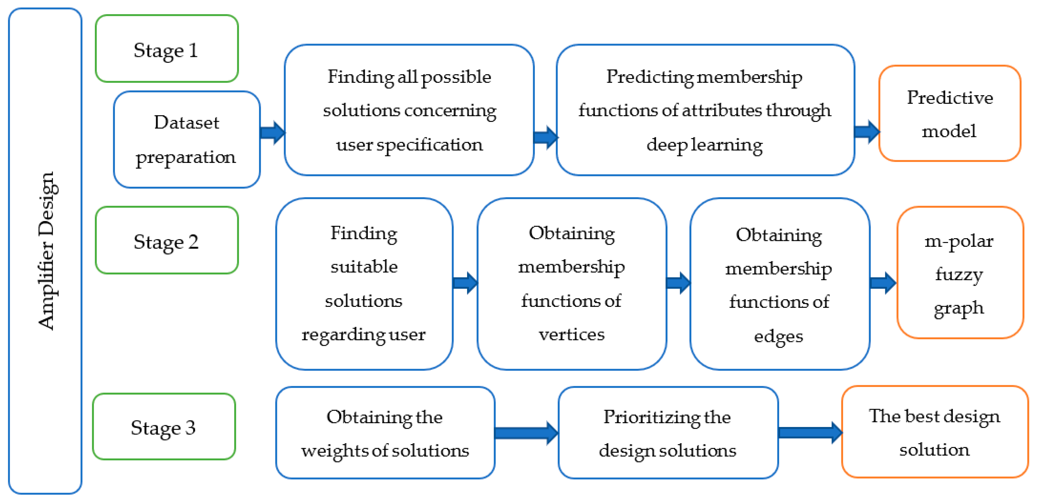
Deep Learning (DL) comprises multiple methods and techniques, based on ANNs, which are utilized for different purposes—from studying a process, event, or facts to analyzing, predicting, or optimizing some parameters. Contemporary surveys summarize approaches, types, and architectures of deep learning algorithms, as well as discuss their applications in the context of supervised, unsupervised, and reinforcement learning [36,37]. The advantages of DL, such as universal usage, robustness, workability with different data types, and scalability are also described. The cases in which DL is suitable for usage are explained to show its usefulness in the unavailability of domain experts, the impossibility to gather the expertise and the complexity of the problem.

In the automation of electronic circuit design, a few papers are devoted to the advantages of ANNs utilization in support of the designers’ tasks.

Dieste-Velasco et al. propose a methodology for assisting the analytical design of analog circuits as it combines the statistical technique factorial design of experiments and ANNs [38]. Such an approach allows the behavioral modelling of circuits to be done with high accuracy.

The work of Devi et al. is focused on the automated design of analog circuits through the usage of ANN-based supervised learning [39]. The method is verified in the design of two different analog circuits and the obtained results are characterized by high accuracy and small mean squared error.

Wang et al. applied deep learning to solve the sizing problem of analog circuits [40]. Two ANNs architectures are proposed, Recurrent Neural Network (RNN) and DL, which are proven to possess the capability to predict the transistor size with high accuracy.

More sophisticated solutions for automating the design process of complex analog systems [41] and for improving the circuit synthesis [42] point out the possibility of reducing the design process resources and decreasing the designer’s effort.

Budak et al. deal with the speed of the design of integrated analog circuits proposing an efficient method for sizing [43]. The method is verified in the design of analog amplifiers and a comparator, and the results show its benefit.

It seems that DL possesses a big potential for the implementation of a supportive, automated, and smart design process that facilitates decision-making and problem-solving. All these advantages and possibilities are considered when choosing the DL for creating predictive models and speeding up the circuit design.

4. Proposed Method

The design of analog amplifiers could be defined as a multi-attribute problem, which is solved here through the utilization of the m-polar fuzzy graphs theory and deep learning. The developed method for amplifier design is presented in Figure 1 and includes three stages:

• In the first stage, a dataset is prepared according to a predefined specification regarding the designed amplifier. All possible variants of the designed electronic circuit are found and membership functions of attributes are predicted through a deep learning algorithm.
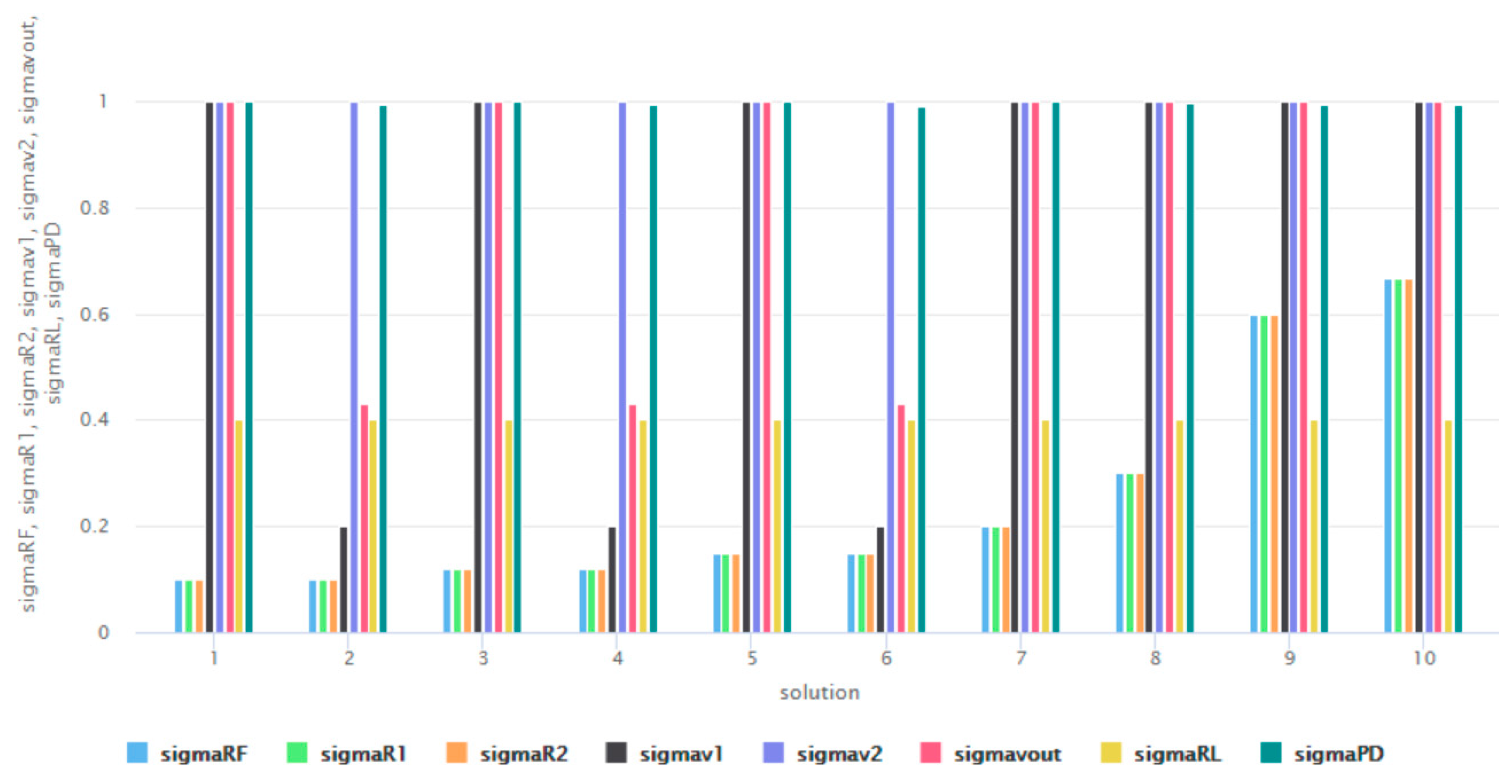
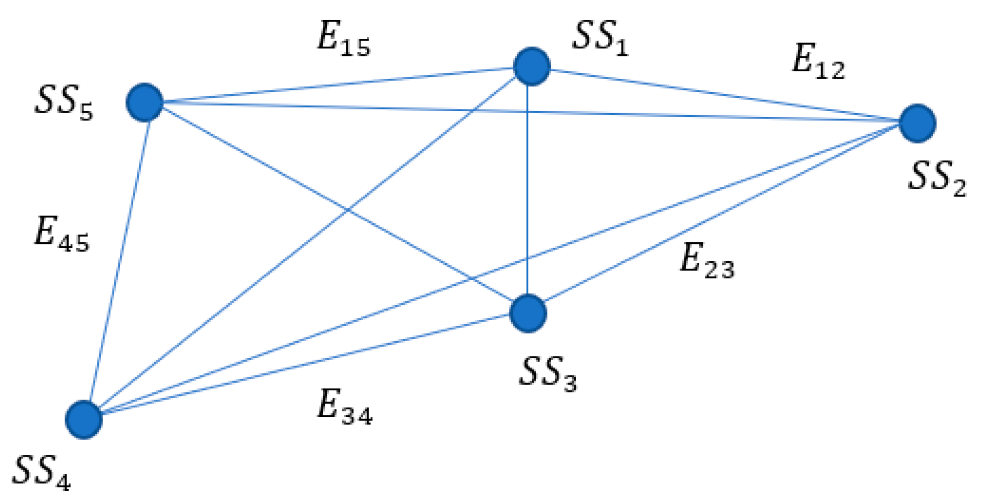
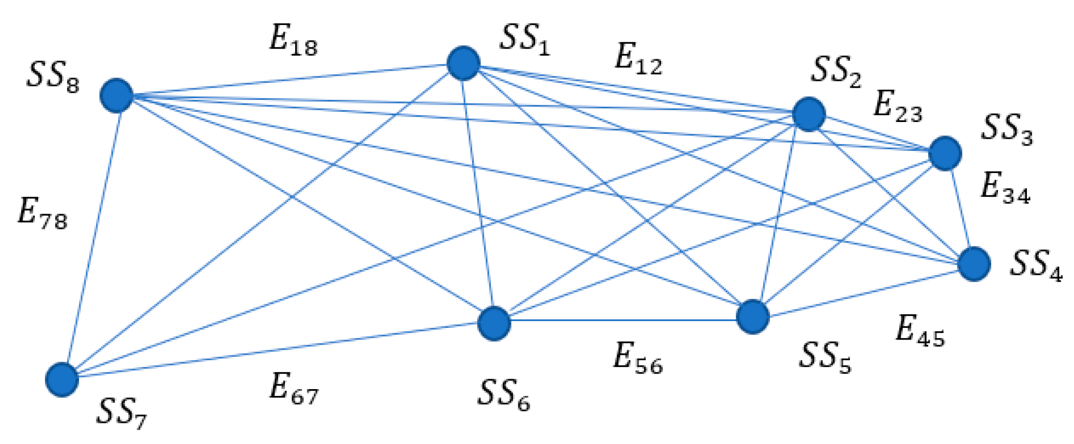
• The second stage points out the suitable design solutions, considering the requested parameters, and after obtaining the membership values of vertices and edges, an m-polar fuzzy graph is constructed.
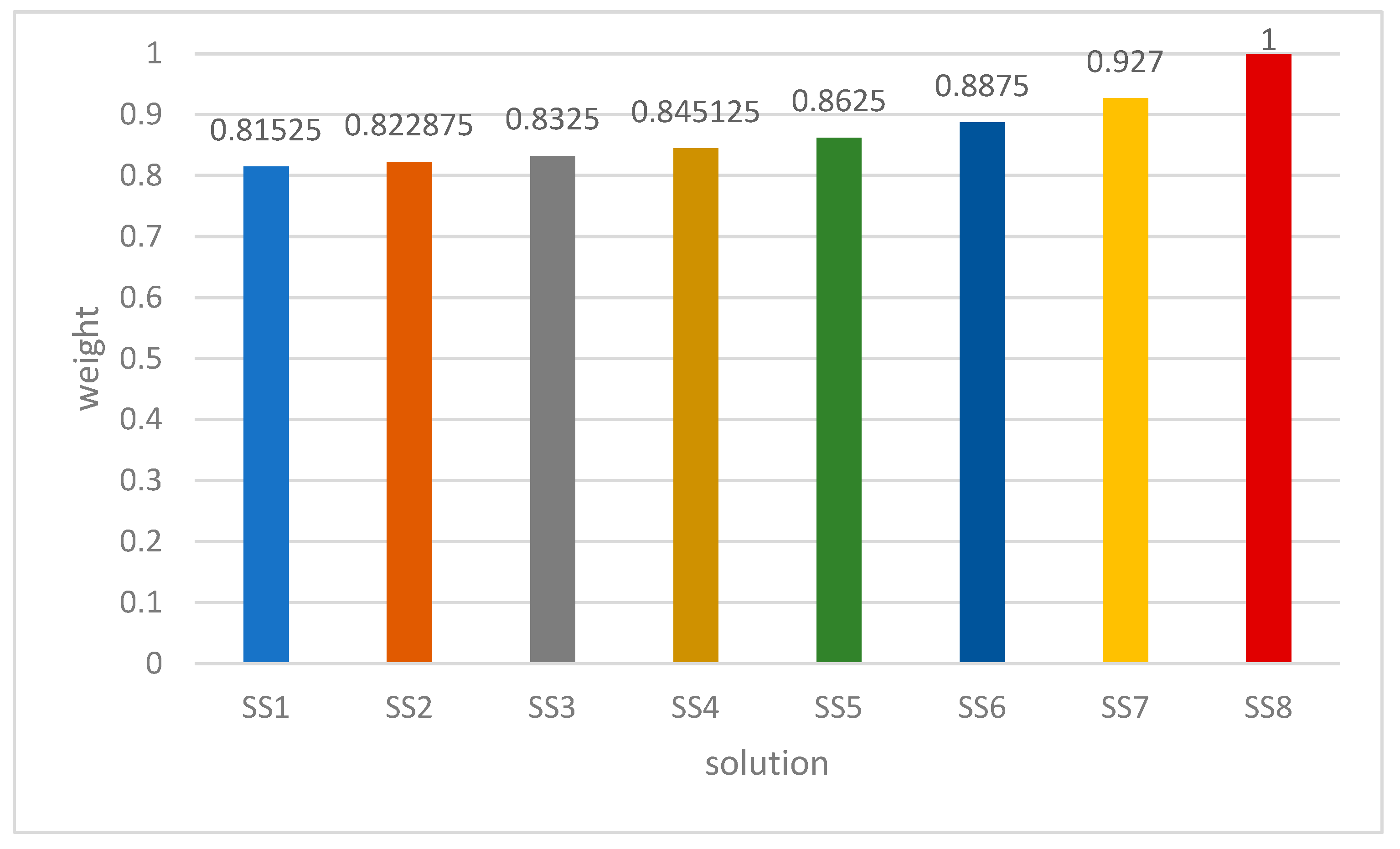
• In the third stage, the most suitable solutions are prioritized, finding the best one, according to the user’s specifications and certain requirements.

5. Experimentation and Results

The problem related to finding the most useful designs of an electronic circuit is examined as a multi-attribute problem for solving. The typical attributes of a given circuit that better explain its electrical and functional behavior are chosen, as they have to be adjusted considering an input specification. For the verification of the proposed method, comprising m-polar fuzzy graphs theory and DL, three electronic circuits are designed: an inverting summing amplifier, a subtracting amplifier (differential amplifier), and a summing/subtracting amplifier with an operational amplifier.

5.1. Design of Inverting Summing Amplifier

Summing amplifiers are very often implemented through operational amplifiers with negative feedback and topology shown in Figure 2. They are used for solving equations such as [44]:

$$v_{out}=-\left(k_1{v}_1+k_2{v}_2+\dots +k_n{v}_n\right)$$

(1)

where scaling coefficients $k_1,k_2, \dots , k_n$ are defined as the ratio between the feedback resistor $R_F$ and the input resistors $R_1, R_2, \dots , R_n$, $v_1, v_2, \dots , v_n$ are input voltage signals, and $v_{out}$ is the output voltage.

One of the challenges for designers is how to satisfy Equation (1), taking into account the possible ranges of input values $v_1, v_2, \dots , v_n$ and output signal $v_{out}$ and considering the allowed range of power dissipation $P_D$typical for the used operational amplifier for a given load $R_L$.

Power dissipation has to possess appropriate values for the normal functioning of the operational amplifier. Otherwise, the operational amplifier will be damaged and the realized analog circuit will not work as expected or will stop working. The amplifier power dissipation $P_D$ is found by knowing the supply voltage $V_S$, maximal quiescent current $I_Q$, output current $I_o$, load current $I_L$, and output voltage $v_{out}$ [45].

The design process of summing amplifiers Is related to finding the values of input resistors $R_1, R_2, \dots , R_n$, taking into account the given scaling coefficients $k_1,k_2, \dots , k_n$ in Equation (1), the output voltage $v_{out}$ at given input voltages $v_1, v_2, \dots , v_n$, and at certain values of the feedback resistor $R_F$ and the load resistor $R_L$.

Let us suppose that the used operational amplifier is OPA 322 [46] and the equation to be solved when designing an inverting summing amplifier, taking into consideration the allowed power dissipation is:

$$v_{out}=-\left(3v_1+6v_2\right)$$

(2)

During the first stage of the proposed method, a dataset in the form of

Table 1. Prepared dataset with possible solutions.

S	${\mathit{R}}_{\mathit{F}},\mathit{k}\mathit{\Omega }$	${\mathit{R}}_1,\mathit{k}\mathit{\Omega }$	${\mathit{R}}_2,\mathit{k}\mathit{\Omega }$	${\mathit{v}}_1,\mathit{V}$	${\mathit{v}}_2,\mathit{V}$	${\mathit{v}}_{\mathit{o}\mathit{u}\mathit{t}},\mathit{V}$	${\mathit{R}}_{\mathit{L}},\mathit{k}\mathit{\Omega }$	${\mathit{P}}_{\mathit{D}},\mathit{m}\mathit{W}$	$\mathit{\sigma }\left({\mathit{P}}_{\mathit{D}}\right)$
$S_1$	60	20	10	0.01	0.01	0.09	10	10.511	0.999
$S_2$	60	20	10	0.05	0.01	0.21	10	10.590	0.992
$S_3$	60	20	10	0.1	0.01	0.36	10	10.684	0.983
$S_4$	60	20	10	0.15	0.01	0.51	10	10.772	0.975
$S_5$	60	20	10	0.2	0.01	0.66	10	10.855	0.968
…		…	…	…	…	…	…	…	…

is prepared, considering a predefined specification. The investigated range of $R_{\mathrm{F}}$ is from $60 \mathrm{k}\mathsf{\Omega }$ to $6 \mathrm{k}\mathsf{\Omega }$, $v_1$ and $v_2$ have values from $0.01V$ to $0.5V$, and $R_L$ takes values from $0.5 \mathrm{k}\mathsf{\Omega }$ to $10 \mathrm{k}\mathsf{\Omega }$. During the design process multiple solutions $S_1, S_2, \dots , S_n$ are possible, which must first be found. All solutions possess common attributes $A_1=R_1, A_2=R_2, A_3=v_1, A_4=v_2, A_5=v_{out}, A_6=R_F,A_7=R_L, A_8=P_D,$ e.g., $S_1=f\left(A_1, A_2, A_3, A_4,A_5,A_6,A_7,A_8\right),$ $S_2=f\left(A_1, A_2, A_3, A_4,A_5,A_6,A_7,A_8\right),$ …, $S_n=f\left(A_1, A_2, A_3, A_4,A_5,A_6,A_7,A_8\right)$.

All obtained solutions are assigned membership values for each attribute ${\sigma }^{S_i}\left(A_j\right)$ corresponding to the membership functions. The created dataset is presented in Table 1 and the last column includes the membership values of power dissipation $P_D$. The membership values of other attributes are not shown, but they are predicted in a similar way through a deep learning algorithm with a regression task. The ANN includes two hidden layers with 50 neurons at each layer. The utilized activation function is Rectifier. The dataset contains 13,090 records, of which 70% are used for training and 30% for testing.

The achieved accuracy of the predictive model is assessed considering standard metrics such as Root mean squared error (RMSE) = 0.0098, Absolute error (AE) = 0.0053, and Relative error (RE) = 0.98%. Figure 3 presents the prediction chart and the linear regression result.

In the second stage, the designer is looking for solutions with maximal membership function of power dissipation$P_D$, e.g., minimal values of power dissipation$P_D$ and allowable values of the rest of the examined attributes. It is found that these requirements are satisfied by 51 of 13,090 designs: $S{S}_1, S{S}_2,.., S{S}_{51}$. The membership functions of vertices (solutions) of the fuzzy graph are predicted through deep learning as ten random solutions are shown in Figure 4. For further exploration, five solutions which are the most appropriate, are considered. Thus, effort and resources are reduced, selecting and examining the closest to the user specification solutions.

An m-polar fuzzy graph is constructed with five vertices (the most suitable five solutions with minimal power dissipation $P_D–S{S}_1, S{S}_2, \dots , S{S}_5$ and edges between them (Figure 5). The membership functions of the edges ($S{S}_i, S{S}_k$), with respect to the attributes $A_1÷A_8$ are found according to the following equation [31] (

Table 2. Membership values of the edges.

$\mathit{S}{\mathit{S}}_{\mathit{i}}\otimes \mathit{S}{\mathit{S}}_{\mathit{k}}$	${\mathit{A}}_1$	${\mathit{A}}_2$	${\mathit{A}}_3$	${\mathit{A}}_4$	${\mathit{A}}_5$	${\mathit{A}}_6$	${\mathit{A}}_7$	${\mathit{A}}_8$
$E_{12}=S{S}_1\otimes S{S}_2$	0.1	0.1	0.1	1	1	1	0.4	0.999
$E_{23}=S{S}_2\otimes S{S}_3$	0.12	0.12	0.12	1	1	1	0.4	0.999
$E_{34}=S{S}_3\otimes S{S}_4$	0.1	0.1	0.1	1	1	1	0.4	0.999
$E_{45}=S{S}_4\otimes S{S}_5$	0.1	0.1	0.1	1	1	1	0.444	0.999
$E_{15}=S{S}_1\otimes S{S}_5$	0.1	0.1	0.1	1	1	1	0.4	0.999
…	…	…	…	…	…	…	…	…

):

$$\mu \left(S{S}_i, S{S}_k\right)={\sigma }^{S{S}_i}\left(A_j\right)\wedge {\sigma }^{S{S}_k}\left(A_j\right)$$

(3)

In the third stage, the membership values of the solutions considering the membership values of every attribute, are calculated through the weight function:

$$w\left(S_i\right)=\frac{\sum {\sigma }^{S{S}_i}\left(A_j\right)}{\mathrm{n}}$$

(4)

where n is the number of attributes.

Figure 6 gives information on the calculated weights of every candidate for the best solution. It seems that the $S{S}_3$ is the best-found design considering the specified requirements. The best design could be used for amplifier prototyping with priorities in comparison to the other four designs.

5.2. Design of Subtracting Amplifier (Differential Amplifier)

The function realized from the subtracting amplifier (differential input amplifier), presented in Figure 7, is described by the following equation [44]:

$$v_{out}=k\left(v_2-v_1\right)$$

(5)

where $k=\frac{R_F}{R_1}$, e.g., the output voltage is proportional to or equal to the difference between the input voltages.

Let us suppose that the specification requires the subtracting amplifier to realize the following function at minimal power dissipation $P_D$:

$$v_{out}=3\left(v_2-v_1\right)$$

(6)

The suggestion is that the used operational amplifier is OPA 322 [46] and the explored range of $R_{\mathrm{F}}$ is from $60 \mathrm{k}\mathsf{\Omega }$ to $3 \mathrm{k}\mathsf{\Omega }$, $v_1$ and $v_2$ have values from $0.01V$ to $0.5V$, $R_L$ takes values from $0.5 \mathrm{k}\mathsf{\Omega }$ to $10 \mathrm{k}\mathsf{\Omega }$. The design solutions are characterized by seven attributes: $A_1=R_1, A_2=v_1, A_3=v_2, A_4=v_{out}, A_5=R_F,A_6=R_L, A_7=P_D,$ e.g., $S_1=f\left(A_1, A_2, A_3, A_4,A_5,A_6,A_7\right),$ $S_2=f\left(A_1, A_2, A_3, A_4,A_5,A_6,A_7\right),$ …, $S_n=f\left(A_1, A_2, A_3, A_4,A_5,A_6,A_7\right)$.

The prepared dataset is similar to Table 1. The membership values of the rest of the attributes are also predicted through a deep-learning algorithm. The learning records are 5710 and the prediction chart of the membership values of power dissipation (sigma) is presented in Figure 8. The created predictive model is characterized by very small errors: RMSE = 0.0032, AE = 0.0022, RE = 0.27%.

Figure 9 depicts the membership values of ten randomly chosen designs.

At the second stage, out of all possible 5710 designs, eight are selected—these with the maximal membership values of power dissipation $P_D$.

For fuzzy graph construction, in addition to the membership values of vertices, it is necessary to know the membership values of the edges, which are calculated similarly to the previous demonstration and are presented in

Table 3. Membership values of the edges.

$\mathit{S}{\mathit{S}}_{\mathit{i}}\otimes \mathit{S}{\mathit{S}}_{\mathit{k}}$	${\mathit{A}}_1$	${\mathit{A}}_2$	${\mathit{A}}_3$	${\mathit{A}}_4$	${\mathit{A}}_5$	${\mathit{A}}_6$	${\mathit{A}}_7$	${\mathit{A}}_8$
$E_{12}=S{S}_1\otimes S{S}_2$	1	1	0.222	0.3	1	1	1	1
$E_{23}=S{S}_2\otimes S{S}_3$	1	1	0.25	0.333	1	1	1	1
$E_{34}=S{S}_3\otimes S{S}_4$	1	1	0.285	0.375	1	1	1	1
$E_{45}=S{S}_4\otimes S{S}_5$	1	1	0.333	0.428	1	1	1	1
$E_{56}=S{S}_5\otimes S{S}_6$	1	1	0.4	0.5	1	1	1	1
$E_{67}=S{S}_6\otimes S{S}_7$	1	1	0.5	0.6	1	1	1	1
$E_{78}=S{S}_7\otimes S{S}_8$	1	1	0.666	0.75	1	1	1	1
…	…	…	…	…	…

. The m-polar fuzzy graph itself is shown in Figure 10. Its structure points out the most suitable designs found, which are eight $S{S}_1÷S{S}_8$. They are connected because they share common attributes.

In the third stage, the best solution found is $S{S}_8$, after calculating the values of the weighting function (ordinate axes) as it is shown in Figure 11. It seems that SS8 is the design, which satisfies the user requirements in the best way. Moreover, the remaining seven also could be applied because of the closest weighting values to the most suitable design.

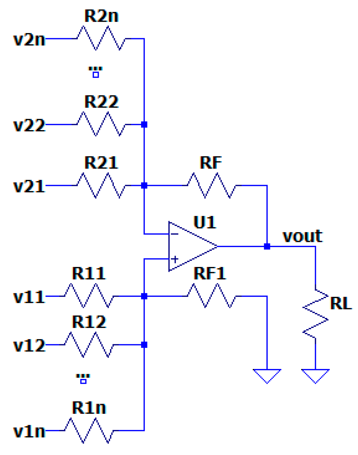
5.3. Summing and Subtracting Amplifier

The electronic circuit of the summing and subtracting amplifier is presented in Figure 12. The output voltage $v_{out}$ is calculated as the sum of the input voltages applied to the non-inverting input $v_{11}, v_{12},\dots ,v_{1n}$, and the subtraction of the input voltages at the inverting input $v_{21},v_{22},\dots ,v_{2n}$. So, the implemented function of this amplifier can be presented in the following form [44]:

$$v_{out}=\left(k_{11}{v}_{11}+k_{12}{v}_{12}+\cdots +k_{1n}{v}_{1n}\right)-\left(k_{21}{v}_{21}+k_{22}{v}_{22}+\cdots +k_{2n}{v}_{2n}\right)$$

(7)

The sizing coefficients are defined as the ratio between the feedback resistor and the respective input resistor $k_{1j}=\frac{R_{F1}}{R_{1j}}$ and $k_{2j}=\frac{R_F}{R_{2j}}$.

If the specification says that the amplifier must satisfy the following equation:

$$v_{out}=\left(9v_{11}+2v_{12}\right)-\left(6v_{21}+3v_{22}\right)$$

(8)

then the first stage includes the dataset preparation, which is similar to the one shown in Table 1 and the aim is the design with minimal power dissipation $P_D$ to be found considering a given load $R_L$. The examined design solutions are 144,414: $S_1÷S_{144414}$ as they possess 11 common attributes: $A_1=R_{\mathrm{F}}, A_2=R_1, A_3=R_2, A_4=R_3, A_5=R_4,A_6=v_1, A_7=v_2, A_8=v_3, A_9=v_4, A_{10}=v_{out},A_{11}=P_D$. All obtained solutions are assigned predicted membership values for each attribute ${\sigma }^{S_i}\left(A_j\right)$ through the usage of a deep learning algorithm. The prediction chart of membership values of power dissipation $P_D$ is presented in Figure 13. The predictive model is evaluated, and it is characterized by very small errors: RMSE = 0.0187, AE = 0.0098, RE = 1.57%.

The membership values of ten random solutions out of 144,414 found solutions are presented in Figure 14.

Stage two includes selecting the most suitable solutions from 144,414 designs. The membership values of the most appropriate 39 designs $S{S}_1÷S{S}_{39}$ are calculated, as well as the membership functions of the edges ($S{S}_i, S{S}_k$) taking into account the attributes $A_1÷A_{11}$. Then, the m-polar fuzzy graph is constructed.

In the third stage, for every attribute, the membership values of the edges between the vertices are calculated and the weights of the solutions are presented in Figure 15. The best solution found is $S{S}_1$ according to the predefined user specification.

6. Conclusions

The paper presents a novel method for supporting the design process of analog amplifiers based on the concepts of m-polar fuzzy graphs and deep learning techniques. For the verification of the proposed method, three electronic circuits are designed: an inverting summing amplifier, a subtracting amplifier (differential amplifier), and a summing/subtracting amplifier with an operational amplifier as the solved problem is related to finding the designs with the smallest power dissipation and performing a certain mathematical function. The findings point out that:

• The synergetic combination of m-polar fuzzy graphs theory and DL leads to obtaining the most suitable solutions only in three stages, extremely reducing the number of repetitive tasks concerning the calculation of the values of designs’ attributes, their comparison, and design selection.
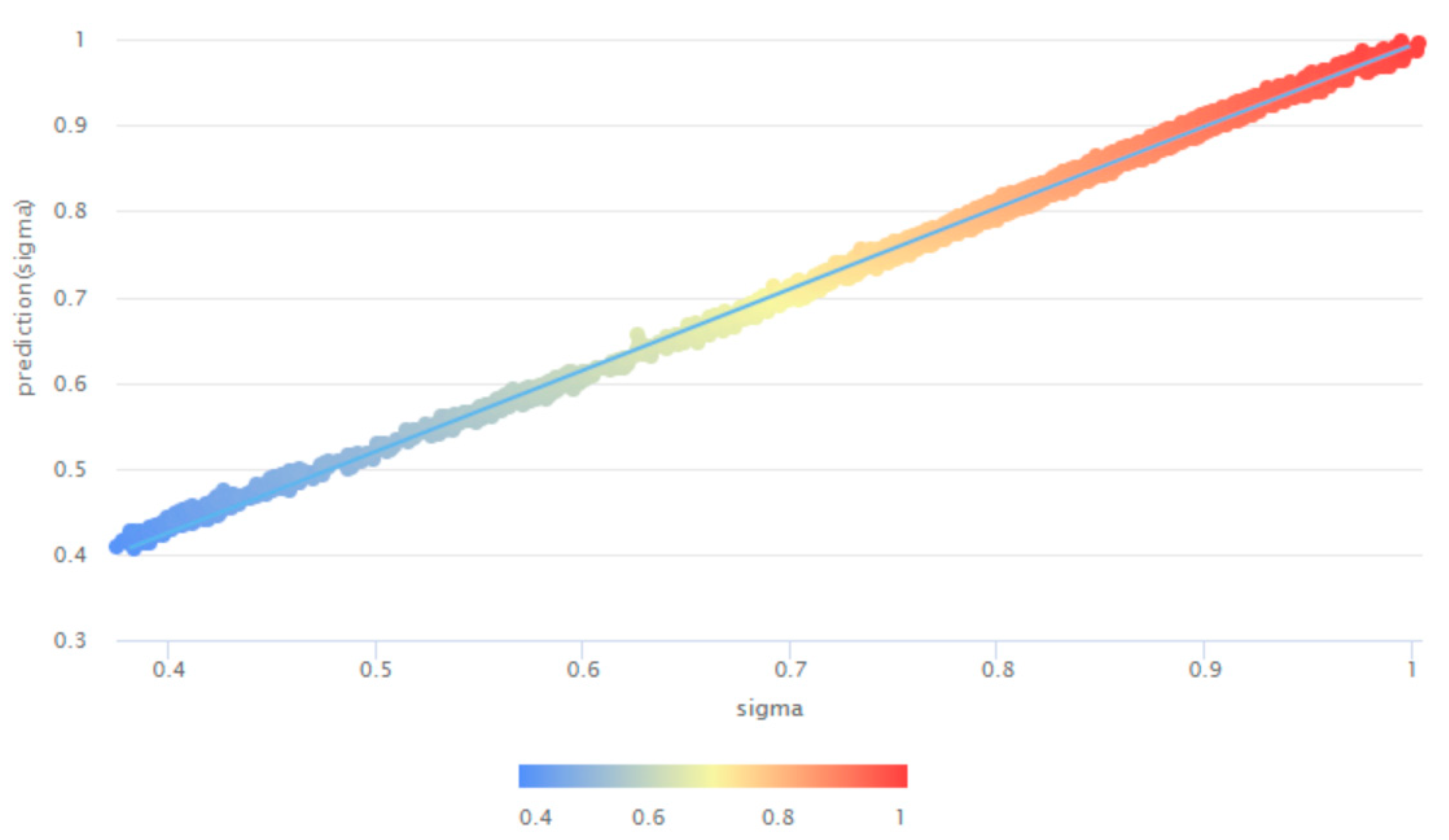
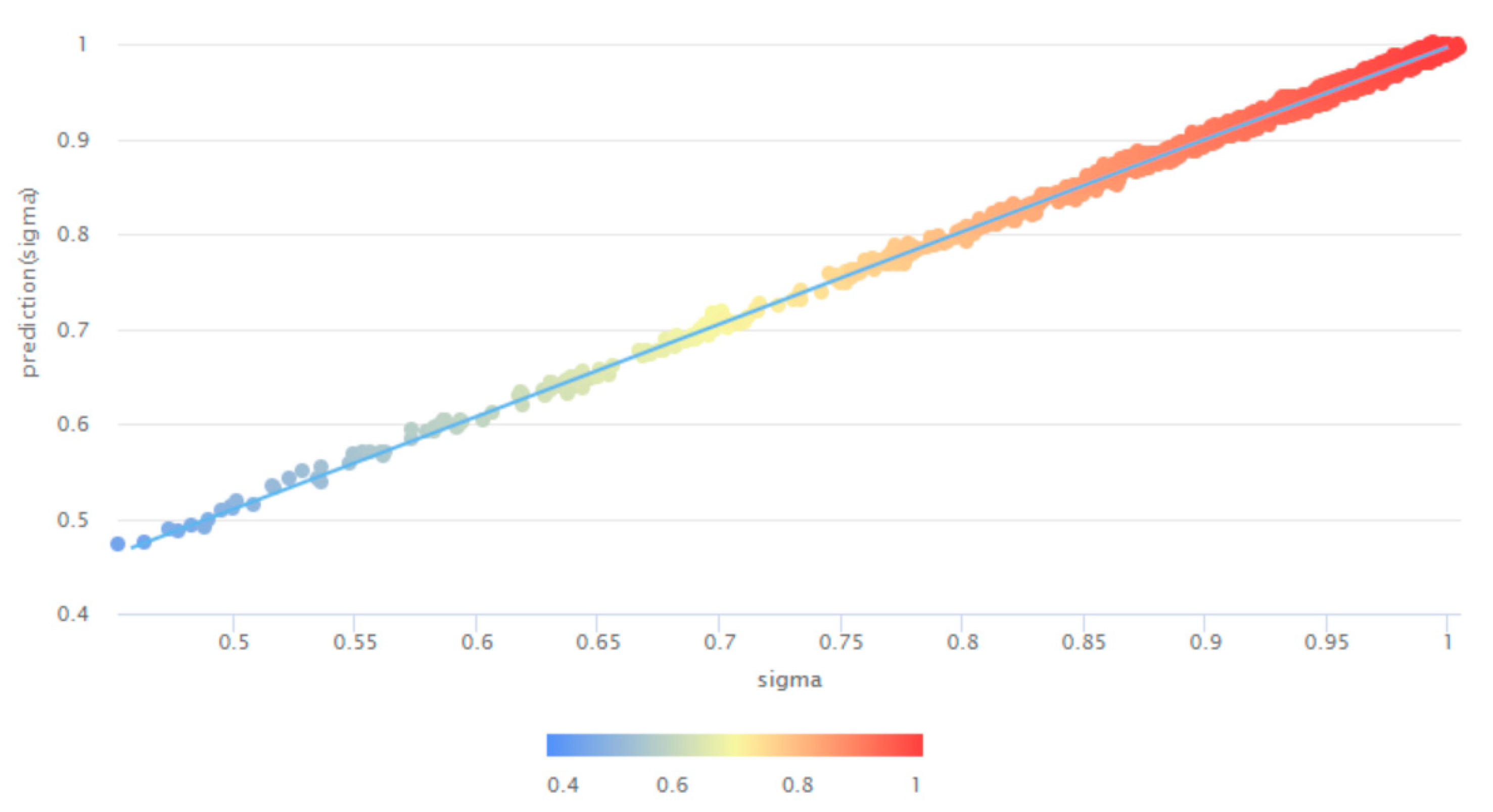
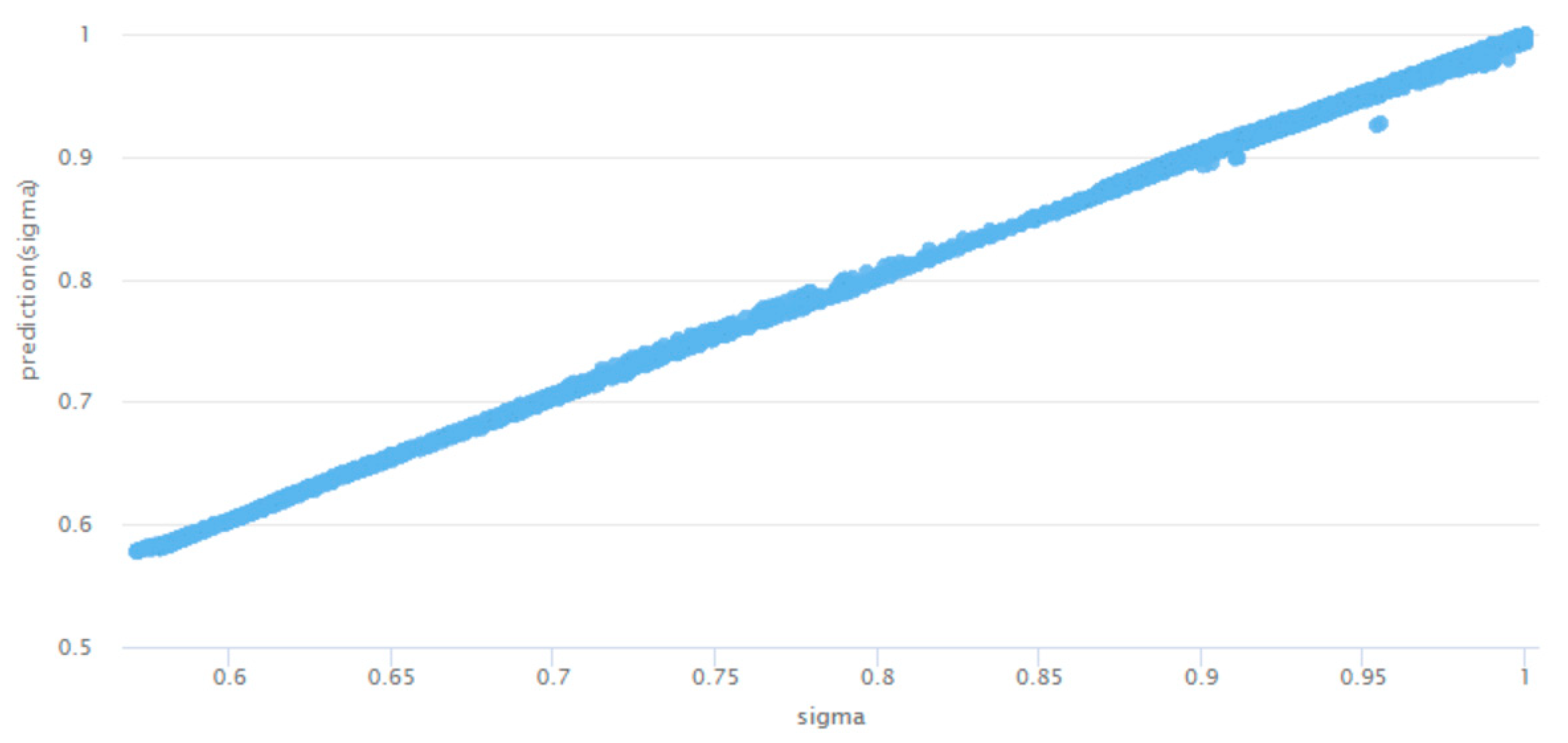
• DL is a suitable approach when expert opinion could be predicted and used for further analysis. In this work, the membership functions of attributes are predicted instead of the expert votes to be gathered. The created predictive models are evaluated, and it is proved that they are characterized with high precision since the obtained errors are very small: RMSE is from 0.0032 to 0.0187, AE is from 0.022 to 0.098, and RE is between 0.27% and 1.57%.
• Fuzzy graph construction gives a possibility for very fast finding the eligible designs, proposes apparatus for their prioritization, and an opportunity for reaching the best design according to a given predefined user specification.

The method can be applied to the design of any electronic circuit to assist a designer in decision-making when the task is multivariate and the environment is complex and uncertain. A promising future work includes further exploration of the advantages and applicability of the m-polar fuzzy graphs theory and deep learning in support of circuit designers and analysts.

References

1. Palomera-Garcia, R. Revisiting Matrix Theory and Electric Circuit Analysis. 2007. Available online: https://www.ineer.org/Events/ICEE2007/papers/140.pdf (accessed on 1 December 2022).
2. Mina, R.; Chadi, J.; Sakr, G.E. A Review of Machine Learning Techniques in Analog Integrated Circuit Design Automation. Electronics 2022, 11, 435. [Google Scholar] [CrossRef]
3. Gao, Y.; He, J. An approach to reducing the time complexity of analog active circuit evolutionary design. In Proceedings of the 2015 11th International Conference on Natural Computation (ICNC), Zhangjiajie, China, 15–17 August 2015; pp. 1098–1102. [Google Scholar] [CrossRef]
4. Zhang, X.; Xia, P.; He, J. Distributed Computation Framework for Circuit Evolutionary Design Under CS Network Architecture. In Proceedings of the 2018 IEEE 18th International Conference on Communication Technology (ICCT), Chongqing, China, 8–11 October 2018; pp. 232–236. [Google Scholar] [CrossRef]
5. Chen, C.-H.; Yang, Y.-S.; Chen, C.-Y.; Hsieh, Y.-C.; Tsai, Z.-M.; Li, Y. Circuit-Simulation-Based Design Optimization of 3.5 GHz Doherty Power Amplifier via Multi-Objective Evolutionary Algorithm and Unified Optimization Framework. In Proceedings of the 2020 IEEE International Symposium on Radio-Frequency Integration Technology (RFIT), Hiroshima, Japan, 2–4 September 2020; pp. 76–78. [Google Scholar] [CrossRef]
6. Fang, Y.; Pong, M.H. A Bayesian Optimization and Partial Element Equivalent Circuit Approach to Coil Design in Inductive Power Transfer Systems. In Proceedings of the 2018 IEEE PELS Workshop on Emerging Technologies: Wireless Power Transfer (Wow), Montreal, QC, Canada, 3–7 June 2018; pp. 1–5. [Google Scholar] [CrossRef]
7. Lyu, W.; Yang, F.; Yan, C.; Zhou, D.; Zeng, X. Batch Bayesian Optimization via Multi-Objective Acquisition Ensemble for Automated Analog Circuit Design. In Proceedings of the 35th International Conference on Machine Learning, Stockholm, Sweden, 10–15 July 2018. [Google Scholar]
8. Li, Q.; Shih, T.-Y. Non-Foster Matching Circuit Synthesis Using Artificial Neural Networks. In Proceedings of the 2021 IEEE Radio and Wireless Symposium (RWS), San Diego, CA, USA, 17–22 January 2021; pp. 11–13. [Google Scholar] [CrossRef]
9. Xuefang, X.; Qinghao, Z.; Yun, L. The Fault Analysis of Analog Circuit Based on BP Neural Network. In Proceedings of the 2021 4th International Conference on Advanced Electronic Materials, Computers and Software Engineering (AEMCSE), Changsha, China, 26–28 March 2021; pp. 128–131. [Google Scholar] [CrossRef]
10. Kaufman, A. Introduction à la Théorie des Sous-Ensembles flous à l’usage des Ingénieurs: Applications à la Linguistique, à la Logique et à la Sémantique; Masson et cie 1: Échandens, Switzerland, 1973. [Google Scholar]
11. Rosenfield, A. Fuzzy graphs. In Fuzzy Sets and Their Application; Zadeh, L., Fu, K., Shimura, M., Eds.; Academic Press: New York, NY, USA, 1975; pp. 77–95. [Google Scholar]
12. Yeh, R.; Bang, S. Fuzzy graphs, fuzzy relations, and their applications to cluster analysis. In Fuzzy Sets and Their Applications; Zadeh, L.A., Fu, K.S., Shimura, M., Eds.; Academic Press: New York, NY, USA, 1975; pp. 125–149. [Google Scholar]
13. Samanta, S.; Pal, M. Fuzzy tolerance graphs. Int. J. Latest Trends Math. 2011, 1, 57–67. [Google Scholar]
14. Samanta, S.; Pal, M. Fuzzy threshold graphs. CIIT Int. J. Fuzzy Syst. 2011, 3, 360–364. [Google Scholar]
15. Pal, M.; Samanta, S.; Rashmanlou, H. Some results on interval-valued fuzzy graphs. Int. J. Comput. Sci. Electron. Eng. 2015, 3, 205–211. [Google Scholar]
16. Pramanik, T.; Samanta, S.; Pal, M. Interval-valued fuzzy planar graphs. Int. J. Mach. Learn. Cybern. 2016, 7, 653–664. [Google Scholar] [CrossRef]
17. Rashmanlou, H.; Pal, M. Balanced interval-valued fuzzy graphs. J. Phys. Sci. 2013, 17, 43–57. [Google Scholar]
18. Samanta, S.; Pal, M. Fuzzy k-competition graphs and p-competition fuzzy graphs. Fuzzy Inform. Eng. 2013, 5, 191–204. [Google Scholar] [CrossRef]
19. Samanta, S.; Akram, M.; Pal, M. M-step fuzzy competition graphs. J. Appl. Math Comput. 2015, 47, 461–472. [Google Scholar] [CrossRef]
20. Javaid, M.; Kashif, A.; Rashid, T. Hesitant Fuzzy Graphs and Their Products. Fuzzy Inf. Eng. 2020, 12, 238–252. [Google Scholar] [CrossRef]
21. Zhang, W. Bipolar fuzzy sets and relations: A computational framework for cognitive modeling and multiagent decision analysis. In Proceedings of the First International Joint Conference of The North American Fuzzy Information Processing Society Biannual Conference. The Industrial Fuzzy Control and Intellige, San Antonio, TX, USA, 18–21 December 1994; pp. 305–309. [Google Scholar]
22. Zhang, W. Bipolar fuzzy sets. In Proceedings of the 1998 IEEE International Conference on Fuzzy Systems Proceedings. IEEE World Congress on Computational Intelligence, Anchorage, AK, USA, 4–9 May 1998; pp. 835–840. [Google Scholar]
23. Akram, M. Bipolar fuzzy graphs. Inf. Sci. 2011, 181, 5548–5564. [Google Scholar] [CrossRef]
24. Chen, J.; Li, S.; Ma, S.; Wang, X. M-polar fuzzy sets: An extension of bipolar fuzzy sets. Sci. World J. 2014, 2014, 416530. [Google Scholar] [CrossRef] [PubMed] [Green Version]
25. Ghorai, G.; Pal, M. A Study on m-polar Fuzzy Planar Graphs. Int. J. Comput. Sci. Math. 2016, 7, 283–292. [Google Scholar] [CrossRef]
26. Ghorai, G.; Pal, M. On some operations and density of m-polar fuzzy graphs. Pac. Sci. Rev. A Nat. Sci. Eng. 2015, 17, 14–22. [Google Scholar] [CrossRef] [Green Version]
27. Ghorai, G.; Pal, M. Some isomorphic properties of m-polar fuzzy graphs with applications. Springer Plus 2016, 5, 2104. [Google Scholar] [CrossRef] [Green Version]
28. Akram, M.; Akmal, R.; Alshehri, N. On m polar fuzzy graph structures. Springer Plus 2016, 5, 1448. [Google Scholar] [CrossRef] [Green Version]
29. Mahapatra, T.; Pal, M. An investigation on m-polar fuzzy tolerance graph and its application. Neural Comput. Appl. 2022, 34, 3007–3017. [Google Scholar] [CrossRef]
30. Akram, M. M-Polar Fuzzy Graphs, Theory, Methods & Applications; Springer Nature Switzerland AG: Cham, Switzerland, 2019. [Google Scholar]
31. Pal, M.; Samanta, S.; Ghorai, G. Modern Trends in Fuzzy Graph Theory; Springer Nature Singapore Pte Ltd.: Singapore, 2020. [Google Scholar]
32. Mathew, S.; Mordeson, J.; Malik, D. Fuzzy Graph Theory; Springer International Publishing: Cham, Switzerland, 2018. [Google Scholar]
33. AL-Hawary, T. Complete fuzzy graphs. Int. J. Math. Comb. 2011, 4, 26–34. [Google Scholar]
34. Bera, S.; Pal, M. On m-Polar Interval-valued Fuzzy Graph and its Application. Fuzzy Inf. Eng. 2020, 12, 71–96. [Google Scholar] [CrossRef]
35. Akram, M.; Sarwar, M. Novel applications of m-polar fuzzy competition graphs in decision support system. Neural Comput. Applic 2018, 30, 3145–3165. [Google Scholar] [CrossRef]
36. Nosratabadi, S.; Mosavi, A.; Keivani, R.; Ardabili, S.; Aram, F. State of the Art Survey of Deep Learning and Machine Learning Models for Smart Cities and Urban Sustainability. In Engineering for Sustainable Future; Várkonyi-Kóczy, A., Ed.; Inter-Academia 2019; Lecture Notes in Networks and Systems; Springer: Cham, Switzerland, 2020; Volume 101. [Google Scholar]
37. Alom, M.Z.; Taha, T.M.; Yakopcic, C.; Westberg, S.; Sidike, P.; Nasrin, M.S.; Asari, V.K. State-of-the-Art Survey on Deep Learning Theory and Architectures. Electronics 2019, 8, 292. [Google Scholar] [CrossRef] [Green Version]
38. Dieste-Velasco, M.I.; Diez-Mediavilla, M.; Alonso-Tristán, C. Regression and ANN Models for Electronic Circuit Design. Complexity 2018, 2018, 7379512. [Google Scholar] [CrossRef]
39. Devi, S.; Tilwankar, G.; Zele, R. Automated Design of An[alog Circuits using Machine Learning Techniques. In Proceedings of the 2021 25th International Symposium on VLSI Design and Test (VDAT), Surat, India, 16–18 September 2021; pp. 1–6. [Google Scholar] [CrossRef]
40. Wang, Z.; Luo, X.; Gong, Z. Application of Deep Learning in Analog Circuit Sizing. In Proceedings of the 2018 2nd International Conference on Computer Science and Artificial Intelligence, Shenzhen, China, 8–10 December 2018; pp. 571–575. [Google Scholar] [CrossRef]
41. Hasani, R.M.; Haerle, D.; Baumgartner, C.F.; Lomuscio, A.R.; Grosu, R. Compositional neural-network modeling of complex analog circuits. In Proceedings of the 2017 International Joint Conference on Neural Networks (IJCNN), Anchorage, AK, USA, 14–19 May 2017; pp. 2235–2242. [Google Scholar] [CrossRef] [Green Version]
42. Dutta, R.; James, A.; Raju, S.; Jeon, Y.J.; Foo, C.S.; Chai, K.T.C. Automated Deep Learning Platform for Accelerated Analog Circuit Design. In Proceedings of the 2022 IEEE 35th International System-on-Chip Conference (SOCC), Belfast, UK, 16 May 2022; pp. 1–5. [Google Scholar] [CrossRef]
43. Budak, A.F.; Gandara, M.; Shi, W.; Pan, D.Z.; Sun, N.; Liu, B. An Efficient Analog Circuit Sizing Method Based on Machine Learning Assisted Global Optimization. IEEE Trans. Comput.-Aided Des. Integr. Circuits Syst. 2022, 41, 1209–1221. [Google Scholar] [CrossRef]
44. Ivanova, M. Analog Electronics; Technical University of Sofia: Sofia, Bulgaria, 2020; ISBN 978-619-167-423-7. (In Bulgarian) [Google Scholar]
45. Kuehl, T. Top Questions on Op Amp Power Dissipation—Part 2; Texas Instruments: Dallas, TX, USA, 2014; Available online: https://e2e.ti.com/blogs_/archives/b/precisionhub/posts/top-2-questions-on-op-amp-power-dissipation-part-2 (accessed on 1 December 2022).
46. Texas Instruments. OPAx322x 20-MHz, Low-Noise, 1.8-V, RRI/O, CMOS Operational Amplifier with Shutdown; Texas Instruments: Dallas, TX, USA, 2016; Available online: https://www.ti.com/lit/ds/symlink/opa322.pdf?ts=1673723341954&ref_url=https%253A%252F%252Fwww.ti.com%252Fproduct%252FOPA322 (accessed on 1 December 2022).
Figure 1. Proposed method.
Mathematics 11 01001 g001
Figure 2. Inverting summing amplifier [44].
Mathematics 11 01001 g002
Figure 3. Prediction chart of the power dissipation P D membership values (sigma) at inverting summing amplifier design.
Mathematics 11 01001 g003
Figure 4. Membership values of ten random solutions at design of inverting summing amplifier.
Mathematics 11 01001 g004
Figure 5. M-polar fuzzy graph at design of inverting summing amplifier.
Mathematics 11 01001 g005
Figure 6. Calculated weights of the solutions at design of the inverting summing amplifier.
Mathematics 11 01001 g006
Figure 7. Subtracting amplifier [44].
Mathematics 11 01001 g007
Figure 8. The prediction chart of the membership values of power dissipation (sigma) at subtracting amplifier design.
Mathematics 11 01001 g008
Figure 9. Membership values of randomly chosen solutions at design of subtracting amplifier.
Mathematics 11 01001 g009
Figure 10. M-polar fuzzy graph at design of subtracting amplifier.
Mathematics 11 01001 g010
Figure 11. Prioritizing the suitable designs of the subtracting amplifier.
Mathematics 11 01001 g011
Figure 12. Summing and subtracting amplifier [44].
Mathematics 11 01001 g012
Figure 13. The prediction chart of the membership values of power dissipation (sigma) at design of summing and subtracting amplifier.
Mathematics 11 01001 g013
Figure 14. Sigma membership values of ten random designs of summing and subtracting amplifier.
Mathematics 11 01001 g014
Figure 15. Prioritizing the suitable designs of the summing and subtracting amplifier.
Mathematics 11 01001 g015