
Mining Significant Utility Discriminative Patterns in Quantitative Databases
Abstract
:1. Introduction
2. Preliminaries and Problem Statement
3. Two-Phase Sampling Procedure
3.1. Overview of the Procedure
| Algorithm 1: HUPSampler |
| Input: D: Dataset [m, M]: the user-specified length interval : minimum utility threshold Output: a random HUP //Step 1: Sampling an integer k 1. Create an ID-tree by scanning D once. 2. For each integer j in [m, M], calculate TUj, TU[m, M] and TU based on ID-tree 3. Draw an integer k in [m, M] based on the utility distribution TUk~TU[m, M] //Step 2: Sampling a HUP 4. Create an ID-tree of RTWUK with random item sequence 5. Randomly return a HUP of length k with utility > based on ID-tree |
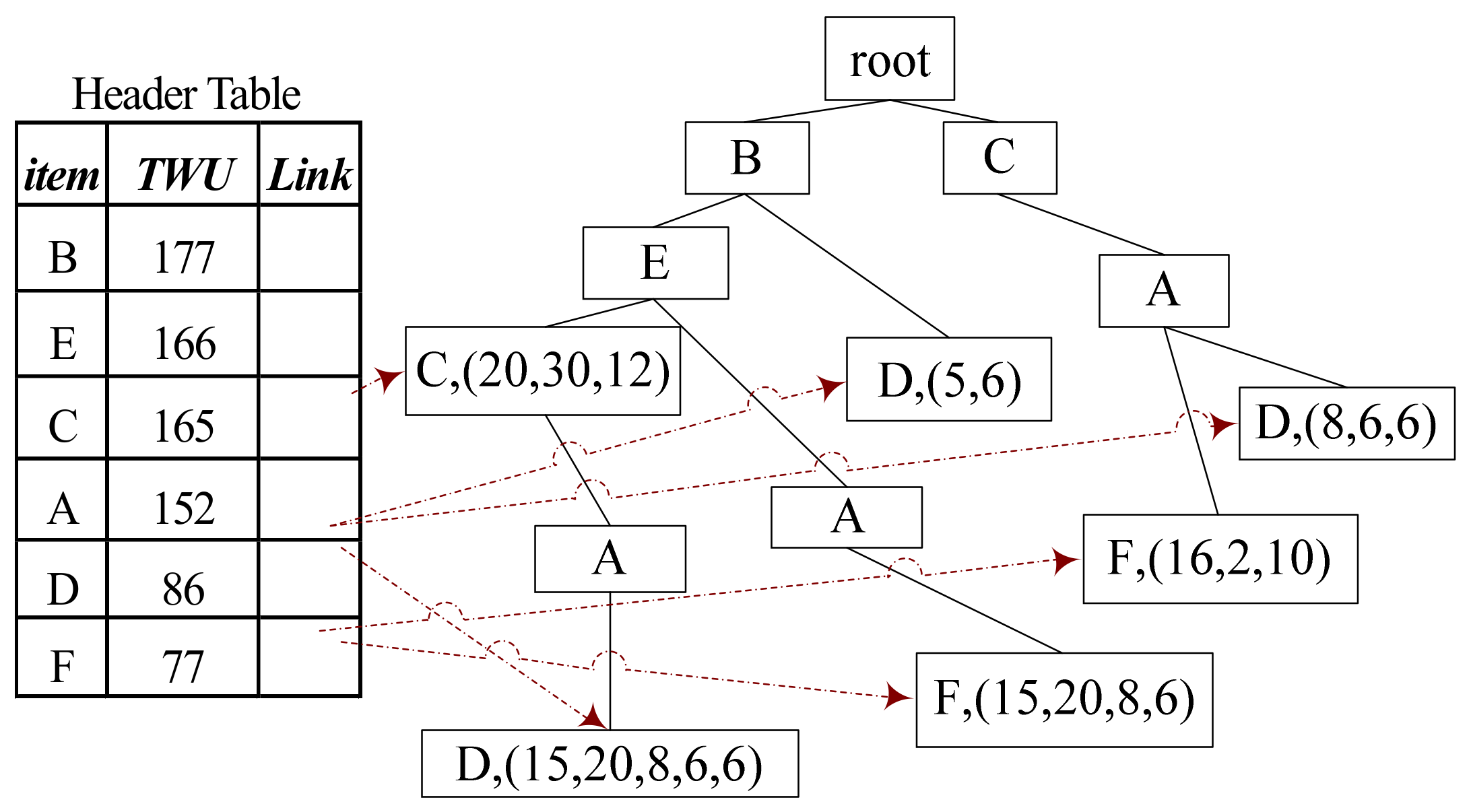
3.2. ID-Tree for Drawing Integer k
3.2.1. Structure of ID-Tree
- .name records the name of the item in ;
- .parent records the parent of ;
- .children records the children of .
- .piu records the utility of the items in the path which is from to the root node. And it can be visited by the indexes of the nodes;
- .bu saves the utility list of base-item which contains the utility of and could be known as a sub set of the path from to the root node.
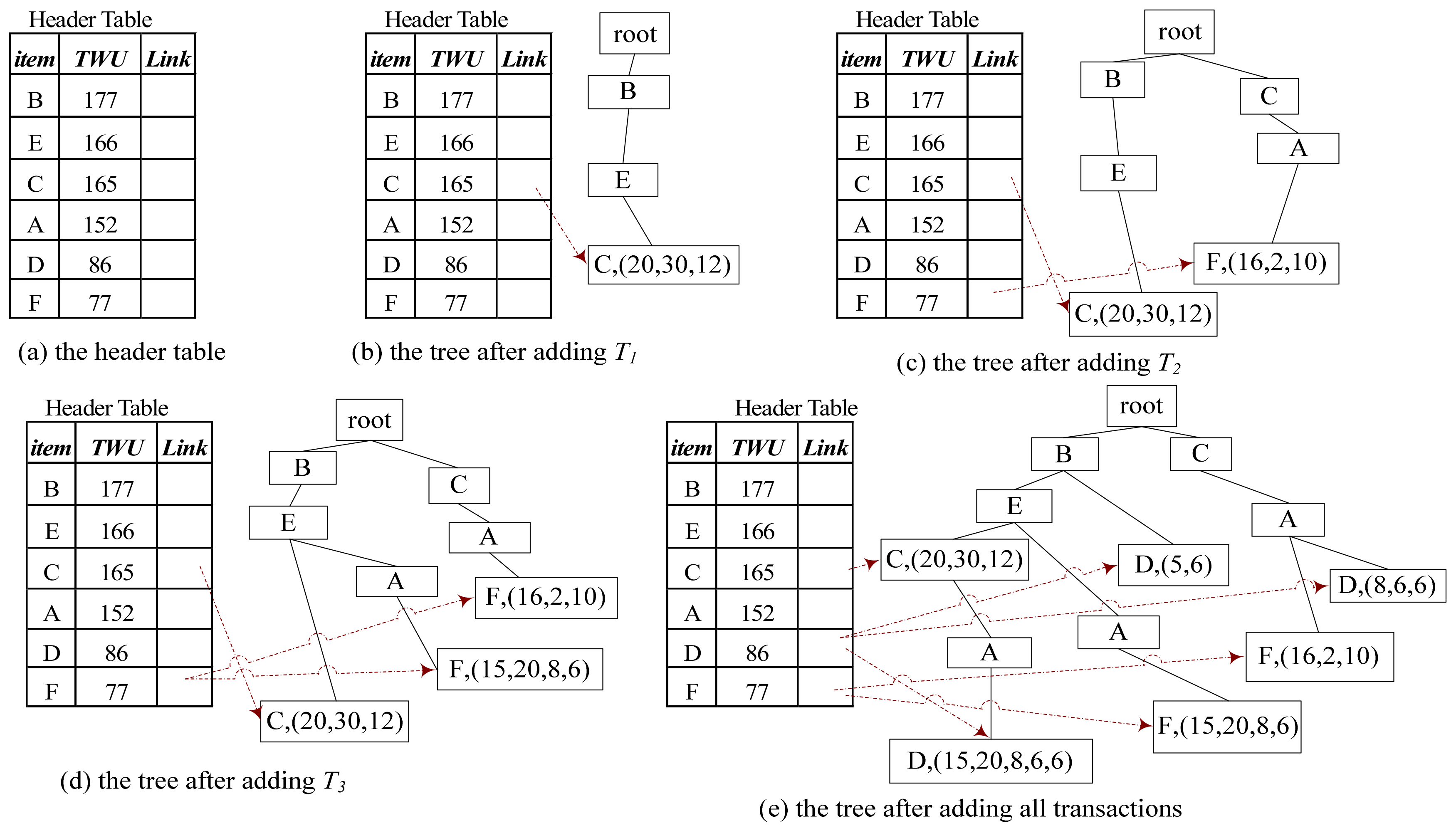
3.2.2. ID-Tree Construction
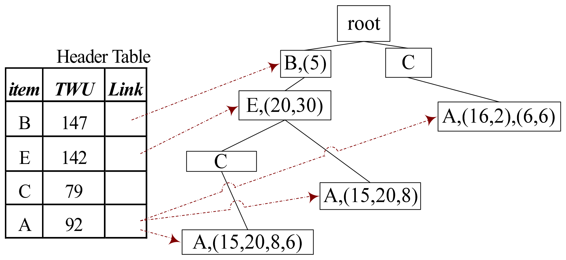
3.2.3. Calculating TU[m, M] and Drawing Integer k Proportionally
| Algorithm 2: CreateTree |
| Input: D: Dataset Output: a ID-tree T 1. For each transaction Td of D do 2. For each item X in Td do 3. Calculate H.X.TWU 4. End For 5. End For 6. Initialize a Tree T with an empty root node, initialize a Table H with TWU descending order 7. T = root() 8. For each transaction Td of D do 9. Insert Td to T with the same descending order of H 10. Add utility to the leaf node 11. Add the links 12. End For 13. Return T |
| Algorithm 3: CalculateTU |
| Input: T: a tree H: a header table m: Minimum length M: Maximum length Dictionary DC Output: TUj (j = m, m + 1, …, M) 1. For each tail node P in H do: 2. base-itemset = Path (P, m, M) 3. If len (base-itemset) ≥ m and len (base-itemset) ≤ M then 4. DC [len (base-itemset)] + =U (base-itemset) 5. End If 6. End For 7. For each tail node P in H do: 8. If P.parent.bu = NULL then 9. P.parent.bu = P.bu 10. P.parent.piu = P.piu 11. else: 12. P.parent.bu + =P.bu 13. P.parent.piu + =P.piu 14. End If 15. Remove P from T 16. End For 17. Create a header table subH 18. CalculateTU (T, subH, m, M,DC) |
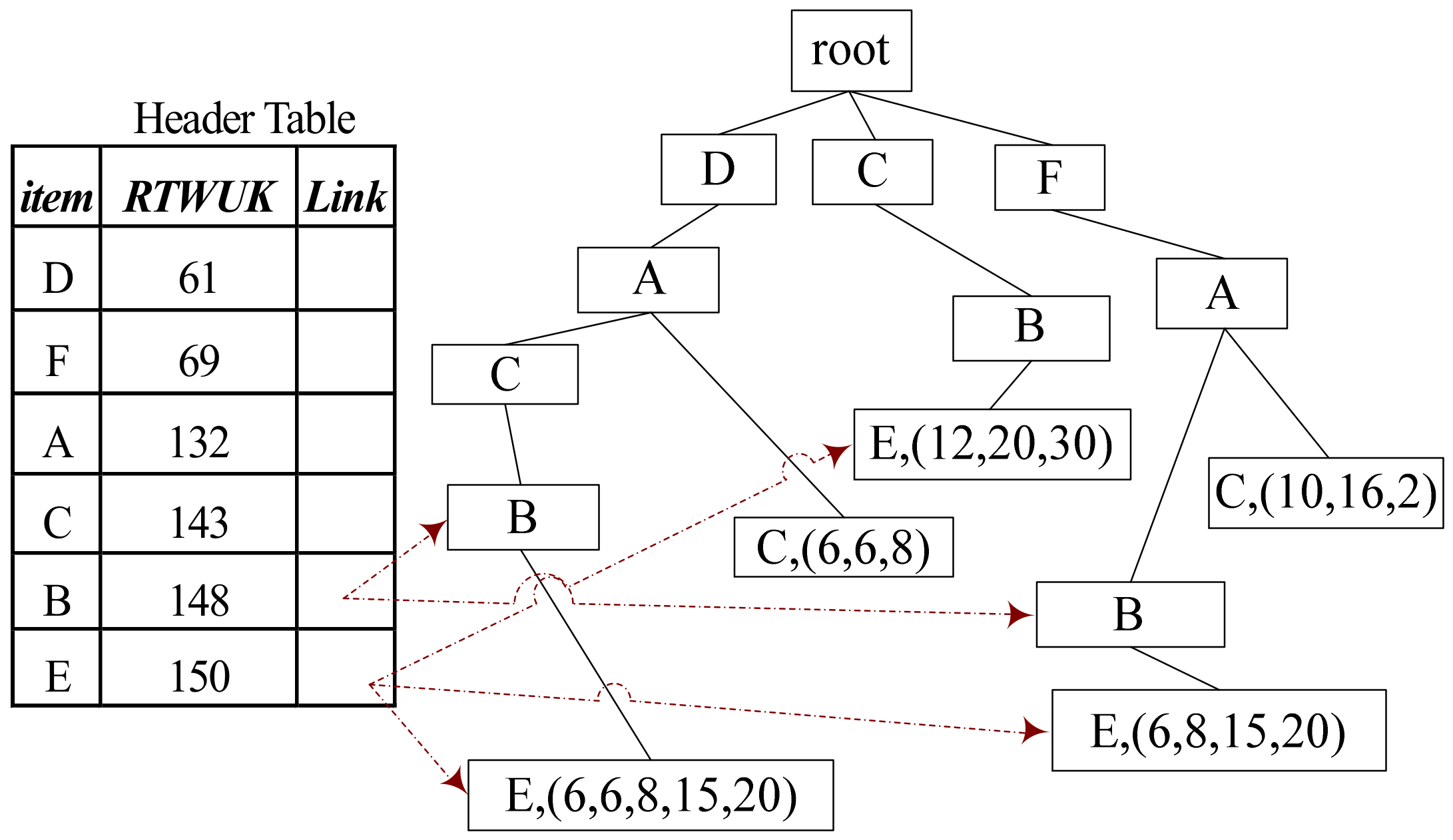
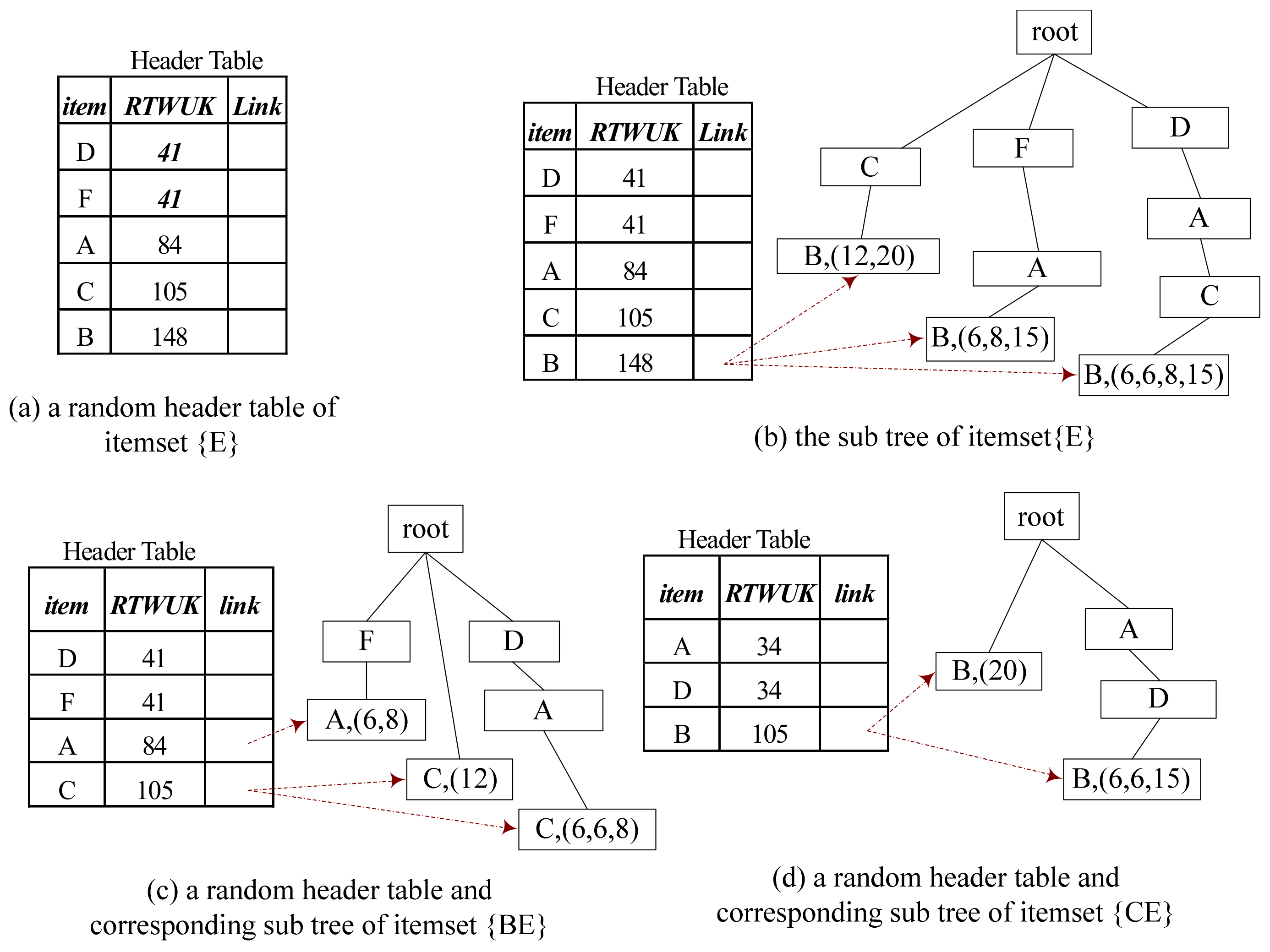
3.2.4. Draw a HUP Uniformly
| Algorithm 4: MHUPK |
| Input: H: a random header table T: a random tree with RTWUK corresponding to H. k: length of pattern MinU: minimum utility value base-item Output: A random HUP of length k 1. For each item P in H (with a bottom-up sequence) do: 2. If H.P.RTWUK ≥ MinU then 3. base-item = base-item {P} 4. If |base-item| = k and H.P.utility ≥ MinU then 5. Break and Return base-item 6. End If 7. If |base-item| < k then 8. Create SubHeader SubH and SubTree SubT 9. MHUPK (subT, subH, k, MinU, base-item) 10. End If 11. Remove P 12. End If 13. End For |
4. Experimental Study
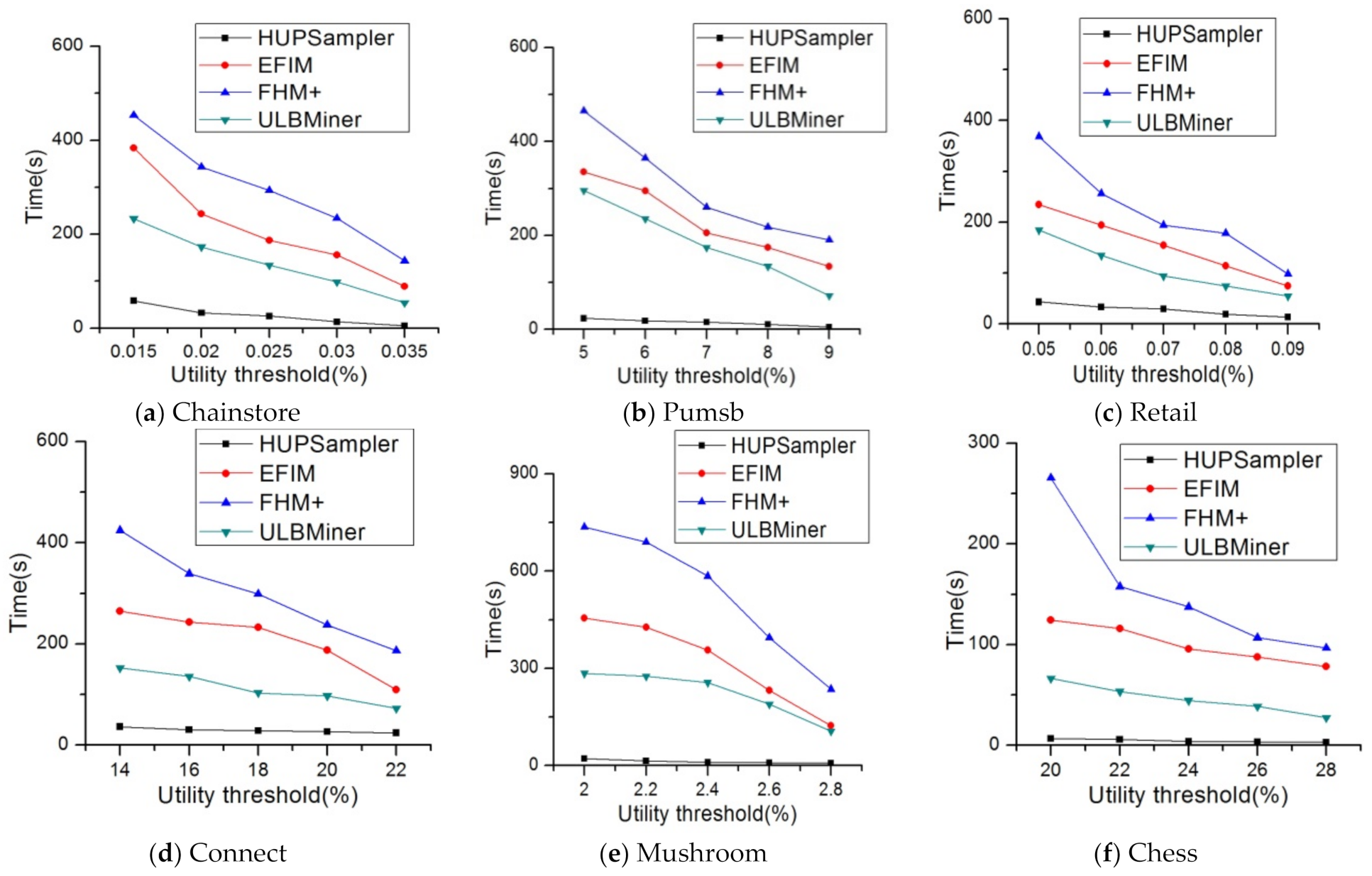
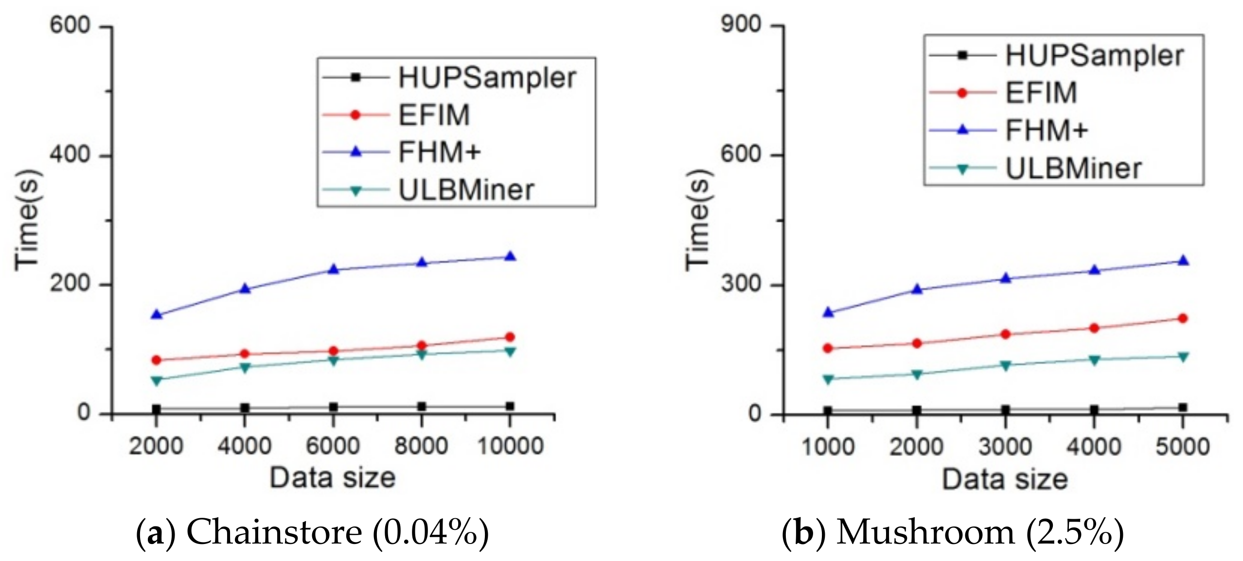
4.1. Running Time
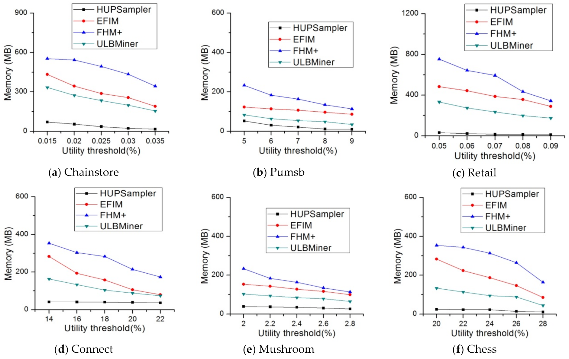
4.2. Memory Usage
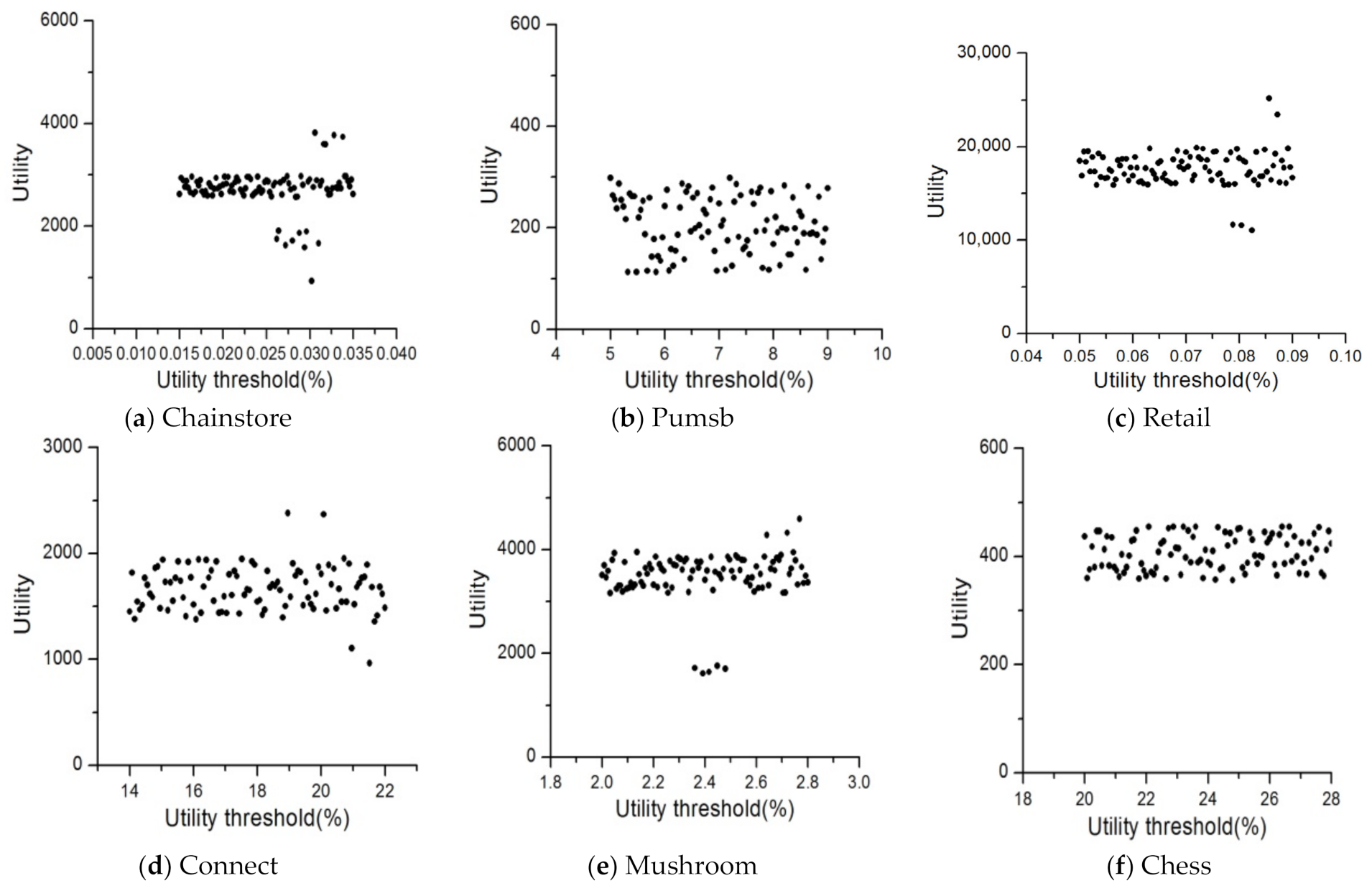
4.3. Utility Distribution
4.4. Case Study
5. Conclusions and Feature Work
Author Contributions
Funding
Institutional Review Board Statement
Informed Consent Statement
Data Availability Statement
Conflicts of Interest
References
- Cheng, J.; Xie, Y.; Zhang, J. Industry structure optimization via the complex network of industry space: A case study of Jiangxi Province in China. J. Clean. Prod. 2022, 338, 130602. [Google Scholar] [CrossRef]
- Wang, E.T.; Chen, A.L. Mining frequent itemsets over distributed data streams by continuously maintaining a global synopsis. Data Min. Knowl. Discov. 2011, 23, 252–299. [Google Scholar] [CrossRef]
- Cheng, J.; Luo, X.W. Analyzing the land leasing behavior of the government of Beijing, China, via the multinomial logit model. Land 2022, 11, 376. [Google Scholar] [CrossRef]
- Tseng, V.; Shie, B.; Wu, C.; Yu, P. Efficient Algorithms for Mining High Utility Itemsets from Transactional Databases. IEEE Trans. Knowl. Data Eng. 2013, 25, 1772–1786. [Google Scholar] [CrossRef]
- Nguyen, H.; Le, N.; Bui, H.; Le, T. A new approach for efficiently mining frequent weighted utility patterns. Appl. Intell. 2022, 53, 121–140. [Google Scholar] [CrossRef]
- Tung, N.T.; Nguyen, L.T.; Nguyen, T.D.; Fourier-Viger, P.; Nguyen, N.T.; Vo, B. Efficient mining of cross-level high-utility itemsets in taxonomy quantitative databases. Inf. Sci. 2022, 587, 41–62. [Google Scholar] [CrossRef]
- Duong, Q.H.; Fournier-Viger, P.; Ramampiaro, H.; Norvag, K.; Dam, T.L. Efficient high utility itemset mining using buffered utility-lists. Appl. Intell. 2018, 48, 1859–1877. [Google Scholar] [CrossRef]
- Fournier-Viger, P.; Wu, C.W.; Souleymane, Z.; Vincent, S. FHM: Faster high-utility itemset mining using estimated utility co-occurrence pruning. In Foundations of Intelligent Systems, 1st ed.; Springer: Cham, Switzerland, 2014; pp. 83–92. [Google Scholar]
- Liu, J.; Wang, K.; Fung, B. Direct Discovery of High Utility Itemsets without Candidate Generation. In Proceedings of the 2012 IEEE 12th International Conference on Data Mining (ICDM), Brussels, Belgium, 10–13 December 2012; pp. 984–989. [Google Scholar]
- Souleymane, Z.; Fournier-Viger, P.; Jerry, C.; Lin, W.; Wu, C.W.; Vincent, S.T. EFIM: A fast and memory efficient algorithm for high-utility itemset mining. Knowl. Inf. Syst. 2017, 51, 595–625. [Google Scholar]
- Liu, M.; Qu, J. Mining high utility itemsets without candidate generation. In Proceedings of the 21st ACM International Conference on Information and Knowledge Management, Maui, HI, USA, 29 October–2 November 2012; pp. 55–64. [Google Scholar]
- Fournier-Viger, P.; Lin, J.C.; Dong, Q.; Dam, T. FHM+: Faster high-utility itemset mining using length upper-bound reduction. In Proceedings of the International Conference on Industrial, Engineering and Other Applications of Applied Intelligent Systems, Berlin/Heidelberg, Germany, 2–4 August 2016; pp. 115–127. [Google Scholar]
- Jenkins, S.; Walzer-Goldfeld, S.; Riondato, M. SPEck: Mining Statistically-significant Sequential Patterns Efficiently with Exact Sampling. Data Mining Knowl. Disc. 2022, 36, 1575–1599. [Google Scholar] [CrossRef]
- Pellegrina, L.; Cousins, C.; Vandin, F.; Riondato, M. McRapper: Monte-Carlo Rademacher Averages for Poset Families and Approximate Pattern Mining. ACM Trans. Knowl. Discov. Data 2022, 16, 124. [Google Scholar] [CrossRef]
- Djenouri, Y.; Comuzzi, M. Combining Apriori heuristic and bio-inspired algorithms for solving the frequent itemsets minin problem. Inf. Sci. 2017, 420, 1–15. [Google Scholar] [CrossRef]
- Pietracaprina, A.; Riondato, M.; Upfal, E.; Vandin, F. Mining top-k frequent itemsets through progressive sampling. Data Min. Knowl. Disc. 2010, 21, 310–326. [Google Scholar] [CrossRef]
- Lin, J.C.W.; Zhang, Y.; Zhang, B.; Fournier-Viger, P.; Djenouri, Y. Hiding sensitive itemsets with multiple objective optimization. Soft Comput. 2019, 23, 12779–12797. [Google Scholar] [CrossRef]
- Tseng, V.S.; Wu, C.W.; Fournier-Viger, P.; Yu, P.S. Efficient Algorithms for Mining Top-K High Utility Itemsets. IEEE Trans. Knowl. Data Eng. 2016, 28, 54–67. [Google Scholar] [CrossRef]
- Yun, U.; Ryang, H.; Ryu, K.H. High utility itemset mining with techniques for reducing overestimated utilities and pruning candidates. Expert Syst. Appl. 2014, 41, 3861–3878. [Google Scholar] [CrossRef]
- Zhang, C.; Zhang, S.; Webb, G.I. Identifying approximate itemsets of interest in large databases. Appl. Intell. 2003, 18, 91–104. [Google Scholar] [CrossRef]
- Gan, W.; Lin, J.C.W.; Zhang, J. Fast utility mining on sequence data. IEEE Trans. Cybern. 2021, 51, 487–500. [Google Scholar] [CrossRef]
- Bashir, S.; Lai, D. Mining Approximate Frequent Itemsets Using Pattern Growth Approach. Inf. Technol. Control 2022, 50, 627–644. [Google Scholar] [CrossRef]
- Yan, C.; Aijun, A. Approximate Parallel High Utility Itemset Mining. Big Data Res. 2016, 6, 26–42. [Google Scholar]
- Diego, S.; Leonardo, P.; Matteo, C.; Fabio, V. SPRISS: Approximating Frequent K-mers by Sampling Reads, and Applications. Bioinformatics 2022, 38, 3343–3350. [Google Scholar]
- Cheng, J. Analysis of the factors influencing industrial land leasing in Beijing of China based on the district-level data. Land Use Policy 2022, 122, 106389. [Google Scholar] [CrossRef]
- Han, Y.; Moghaddam, M. Analysis of sentiment expressions for user-centered design. Expert Syst. Appl. 2021, 171, 114604. [Google Scholar] [CrossRef]
- Yin, P.; Cheng, J. A MySQL-based software system of urban land planning database of Shanghai in China. CMES-Comp. Model Eng. 2023, 135, 2387–2405. [Google Scholar] [CrossRef]
- Fournier-Viger, P.; Gomariz, A.; Gueniche, T. Spmf: A java open source pattern mining library. J. Mach. Learn. Res. 2014, 15, 3389–3393. [Google Scholar]
- Diop, A.; Giacometti, D.; Li, A.S. Sequential Pattern Sampling with Norm Constraints. In Proceedings of the IEEE International Conference on Data Mining (ICDM), Singapore, 17–20 November 2018; pp. 89–98. [Google Scholar]
- Diop, L. High Average-Utility Itemset Sampling Under Length Constraints. In Proceedings of the 26th Pacific-Asia Conference on Knowledge Discovery and Data Mining, Berlin/Heidelberg, Germany, 16–19 May 2022; pp. 134–148. [Google Scholar]
- Wang, L. An Algorithm for Mining Fixed-Length High Utility Itemsets. In Lecture Notes in Computer Science, 1st ed.; Springer: Cham, Switzerland, 2022; pp. 3–20. [Google Scholar]
- Ahmed, C.F.; Tanbeer, S.K.; Jeong, B.S.; Lee, Y.K. Efficient Tree Structures for High Utility Pattern Mining in Incremental Databases. IEEE Trans. Knowl. Data Eng. 2009, 21, 1708–1721. [Google Scholar] [CrossRef]
- Li, Y.C.; Yeh, J.S.; Chang, C.C. Isolated items discarding strategy for discovering high utility itemsets. Data Knowl. Eng. 2008, 64, 198–217. [Google Scholar] [CrossRef]
- Cheng, J.; Yin, P. Analysis of the complex network of the urban function under the lockdown of COVID-19: Evidence from Shenzhen in China. Mathematics 2022, 10, 2412. [Google Scholar] [CrossRef]


| Transaction | |
|---|---|
| T1 | (B, 4) (C, 3) (E, 3) |
| T2 | (A, 1) (C, 4) (F, 10) |
| T3 | (A, 4) (B, 3) (E, 2) (F, 6) |
| T4 | (B, 1) (D, 1) |
| T5 | (A, 3) (B, 3) (C, 2) (D, 1) (E, 2) |
| T6 | (A, 3) (C, 2) (D, 1) |
| Item | A | B | C | D | E | F |
|---|---|---|---|---|---|---|
| Profit | 2 | 5 | 4 | 6 | 10 | 1 |
| Symbol | Definition |
|---|---|
| HUP | High utility pattern |
| HUPK | High utility pattern of length k |
| D | Transactional Dataset |
| Td | dth transaction in D |
| HUP[m, M] | Set of patterns with length in [m, M] |
| MHUPK | Algorithm of mining HUPK |
| TU[m, M] | Sum list of transaction utility with length in [m, M] |
| TWU | Transaction-weighted utility value of D |
| RTWUK | The maximum utility of patterns of length k in D |
| TUk | Sum of transaction utility of length k |
| U(X) | Utility of pattern X |
| U(Td) | Utility of transaction Td |
| Minimum utility threshold | |
| ID-tree | A utility tree |
| m | Minimum lengthof HUP |
| M | Maximum length of HUP |
| Length j | TUj | TU[2,j] |
|---|---|---|
| 2 | 570 | 570 |
| 3 | 587 | 1157 |
| 4 | 269 | 1426 |
| 5 | 55 | 1481 |
| Item | A | B | C | D | E | F |
|---|---|---|---|---|---|---|
| RTWUK | 132 | 148 | 143 | 61 | 150 | 69 |
| Rank | HUP | Utility |
|---|---|---|
| 1 | {BCE} | 105 |
| 2 | {ABE} | 84 |
| 3 | {BEF} | 41 |
| 4 | {BDE} | 41 |
| 5 | {ACD} | 40 |
| 6 | {ACE}, {CDE} | 34 |
| 7 | {ADE} | 32 |
| Dataset | Distinct Items (#) | Average Length | Transactions (#) |
|---|---|---|---|
| Chainstore | 46,086 | 7.2 | 1,112,949 |
| Pumsb | 2111 | 74 | 49,046 |
| Retail | 16,470 | 10.3 | 88,162 |
| Connect | 129 | 43 | 67,557 |
| Mushroom | 119 | 23 | 8124 |
| Chess | 76 | 37 | 3196 |
| Datasets | Minimum Utility Threshold (%) | Running Time (s) | Memory Usage (MB) |
|---|---|---|---|
| Chainstore | 0.015 | 58.4 | 70.1 |
| 0.02 | 32.6 | 53.8 | |
| 0.025 | 25.6 | 35.6 | |
| 0.03 | 13.5 | 21.8 | |
| 0.035 | 5.3 | 15.8 | |
| Pumsb | 5 | 23.5 | 52.5 |
| 6 | 18.5 | 30.7 | |
| 7 | 15.3 | 21.5 | |
| 8 | 10.5 | 11.5 | |
| 9 | 4.9 | 10.4 | |
| Retail | 0.05 | 43.3 | 30.6 |
| 0.06 | 33.5 | 21.6 | |
| 0.07 | 29.5 | 15.6 | |
| 0.08 | 19.6 | 11.7 | |
| 0.09 | 13.4 | 10.5 | |
| Connect | 14 | 36.5 | 41.3 |
| 16 | 30.6 | 40.6 | |
| 18 | 28.7 | 40.1 | |
| 20 | 26.5 | 38.7 | |
| 22 | 24.3 | 36.5 | |
| Mushroom | 2.0 | 22.2 | 38.8 |
| 2.2 | 14.5 | 36.9 | |
| 2.4 | 9.9 | 34.4 | |
| 2.6 | 8.4 | 30.4 | |
| 2.8 | 7.1 | 26.1 | |
| Chess | 20 | 6.7 | 23.9 |
| 22 | 5.9 | 22.2 | |
| 24 | 4.0 | 21.9 | |
| 26 | 3.6 | 13.8 | |
| 28 | 2.8 | 10.7 |
| Dataset | Length Constraints | |||||
|---|---|---|---|---|---|---|
| (10, 20) | (10, 30) | (10, 40) | (10, 50) | (10, 60) | (10, 70) | |
| Chainstore | 0.913 | 0.933 | 0.934 | 0.954 | 0.964 | 0.966 |
| Pumsb | 0.892 | 0.912 | 0.923 | 0.925 | 0.931 | 0.931 |
| Retail | 0.873 | 0.895 | 0.904 | 0.905 | 0.912 | 0.921 |
| Connect | 0.852 | 0.874 | 0.883 | 0.883 | 0.893 | 0.902 |
| Mushroom | 0.812 | 0.823 | 0.835 | 0.836 | 0.846 | 0.875 |
| Chess | 0.823 | 0.832 | 0.843 | 0.851 | 0.861 | 0.863 |
| Minimum Utility Threshold | Proportion (k < 3) | Proportion (3 ≤ k ≤ 5) | Proportion (k > 5) | Average Utility |
|---|---|---|---|---|
| 0.25 | 23% | 61% | 16% | 34.6 |
| 0.5 | 35% | 57% | 8% | 134.4 |
| 0.75 | 12% | 86% | 2% | 125.6 |
| Top 10 Places with High Utility | Average Utility |
|---|---|
| Xiao Guo Zhuang | 212.6 |
| Liu Jia Zuo | 178.5 |
| Shi Jia Zhuang 5th Hospital | 126.4 |
| Xin Le Hospital | 87.6 |
| Xiao Guo Zhuang Primary School | 75.8 |
| Gao Cheng Hospital | 70.9 |
| No. 7 Middle School | 67.5 |
| Hao Yun Lai Restaurant | 60.8 |
| Zeng Cun | 58.6 |
| Ou Jing Yuan | 50.6 |
Disclaimer/Publisher’s Note: The statements, opinions and data contained in all publications are solely those of the individual author(s) and contributor(s) and not of MDPI and/or the editor(s). MDPI and/or the editor(s) disclaim responsibility for any injury to people or property resulting from any ideas, methods, instructions or products referred to in the content. |
© 2023 by the authors. Licensee MDPI, Basel, Switzerland. This article is an open access article distributed under the terms and conditions of the Creative Commons Attribution (CC BY) license (https://creativecommons.org/licenses/by/4.0/).
Share and Cite
Tang, H.; Wang, J.; Wang, L. Mining Significant Utility Discriminative Patterns in Quantitative Databases. Mathematics 2023, 11, 950. https://doi.org/10.3390/math11040950
Tang H, Wang J, Wang L. Mining Significant Utility Discriminative Patterns in Quantitative Databases. Mathematics. 2023; 11(4):950. https://doi.org/10.3390/math11040950
Chicago/Turabian StyleTang, Huijun, Jufeng Wang, and Le Wang. 2023. "Mining Significant Utility Discriminative Patterns in Quantitative Databases" Mathematics 11, no. 4: 950. https://doi.org/10.3390/math11040950