
Station Layout Optimization and Route Selection of Urban Rail Transit Planning: A Case Study of Shanghai Pudong International Airport
Abstract
:1. Introduction
- (1)
- Preliminary analysis of passenger flow, emphasizing layout form and ignoring operational efficiency, results in narrow station spacing and the passenger flow far below expectations;
- (2)
- Local governments are affected by the image project when encountering network planning and administrative intervention, or the adjustment of rail transit planning due to the change of local leaders is relatively standard;
- (3)
- The increase in government debt is caused by excessive investment.
- (1)
- This paper combines urban rail transit planning and HDBSCAN algorithm to present some suggestions and specific route schemes for the local government to scientifically plan rail transit lines.
- (2)
- This paper comprehensively considers the construction cost, operating cost, social benefits, land development value-added along the Metro line and travel time cost of passengers, and proposes a more complete optimization model of station spacing.
- (3)
- The method for studying the station layout, which integrates station spacing, ideal location and spatial analysis optimization, is pioneering and can provide a reference for developing rail transit in metropolises.
- (4)
- This paper selects data points in high-population areas for analysis, and the layout planning of rail transit stations based on this dataset can relieve the traffic pressure of community residents and guarantee all-age-friendly travel in the community.
2. Analysis of Influencing Factors on Layout Optimization of Rail Transit Stations
2.1. Influencing Factors of Station Spacing
- (1)
- The salaries of operating personnel;
- (2)
- The cost of equipment update and maintenance;
- (3)
- The cost of daily purchase of power and other resources.
2.2. Influencing Factors of Station Selection
3. Analysis of Influencing Factors on Layout Optimization of Rail Transit Stations
3.1. The Optimization Model of Station Spacing
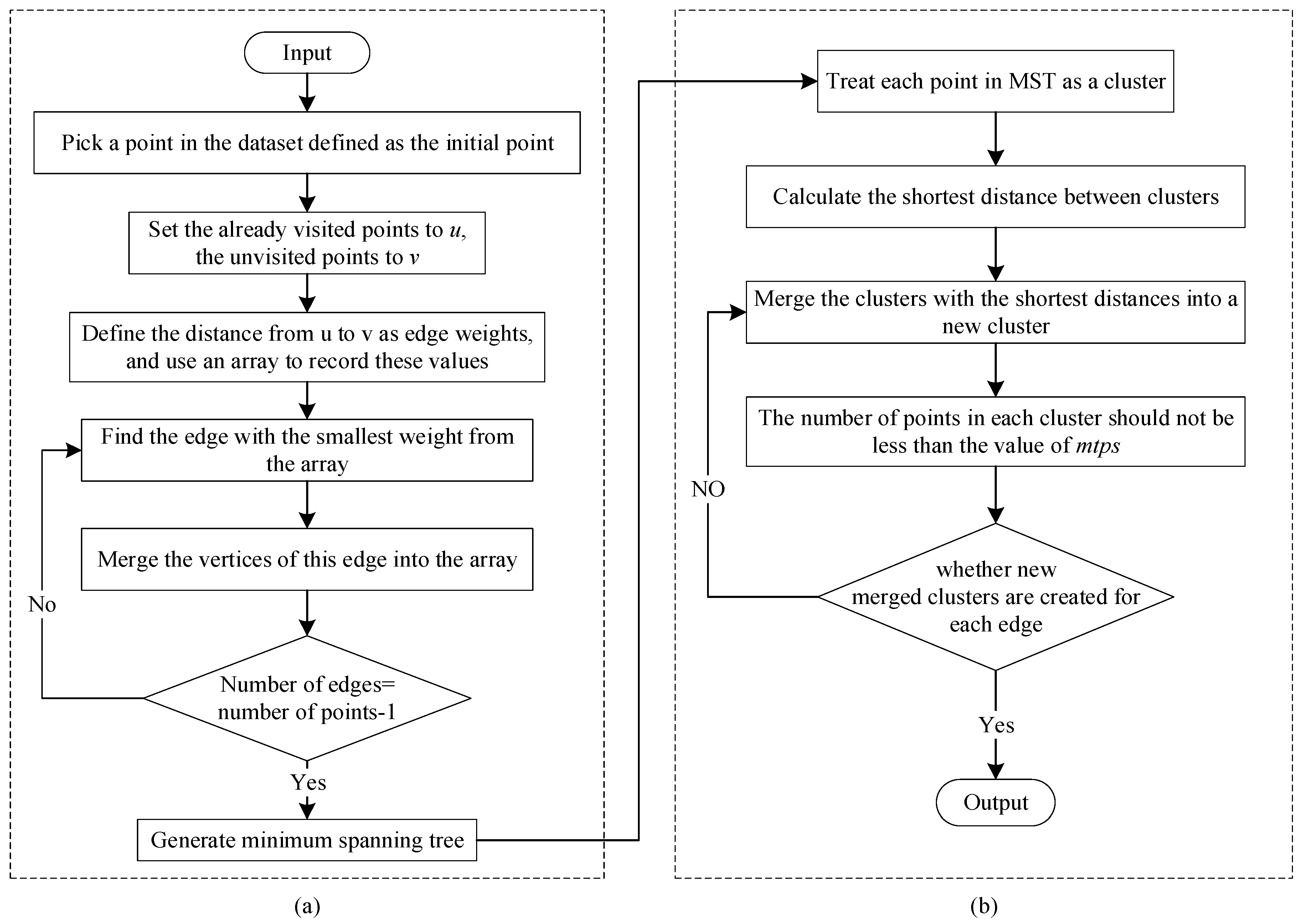
3.2. HDBSCAN Algorithm
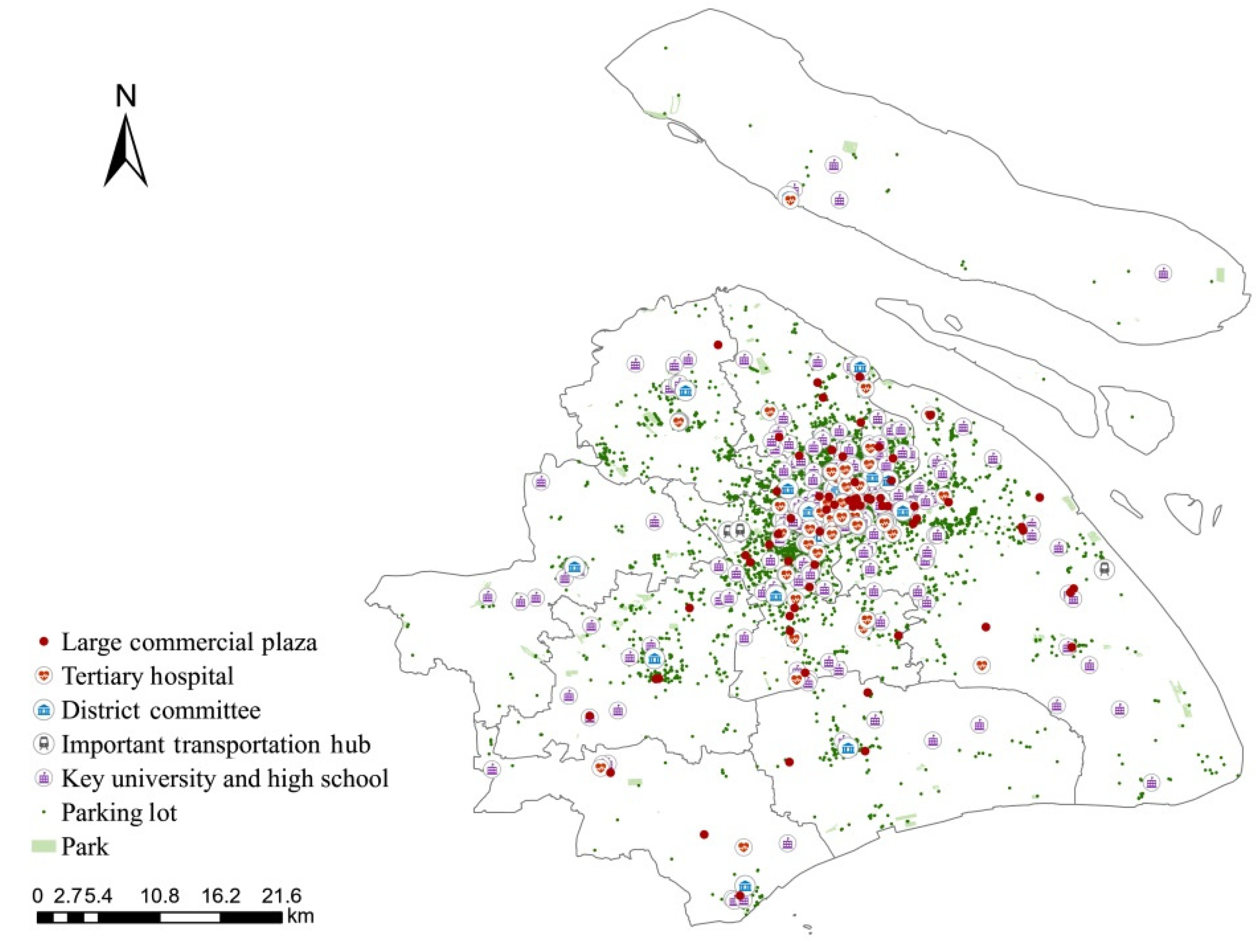
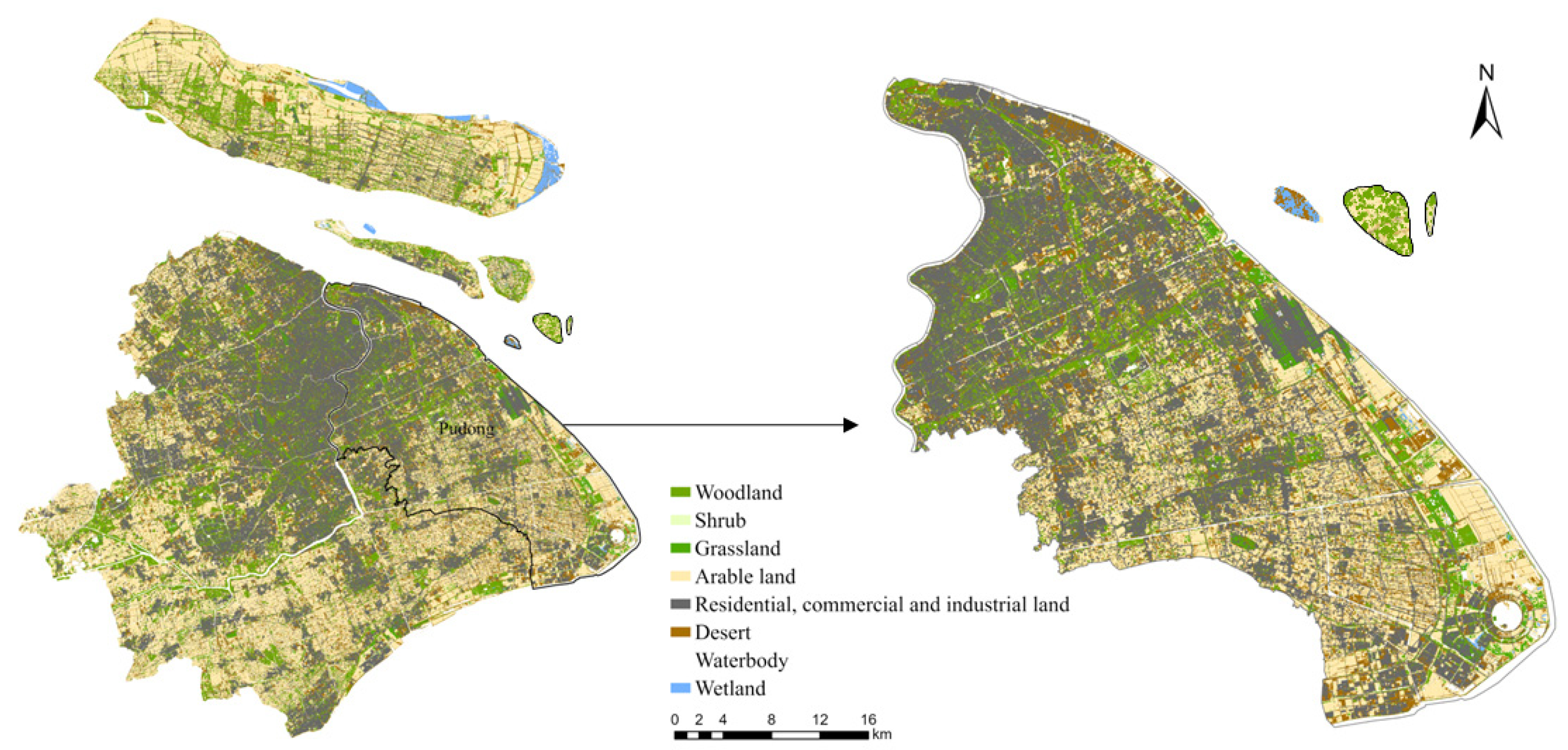
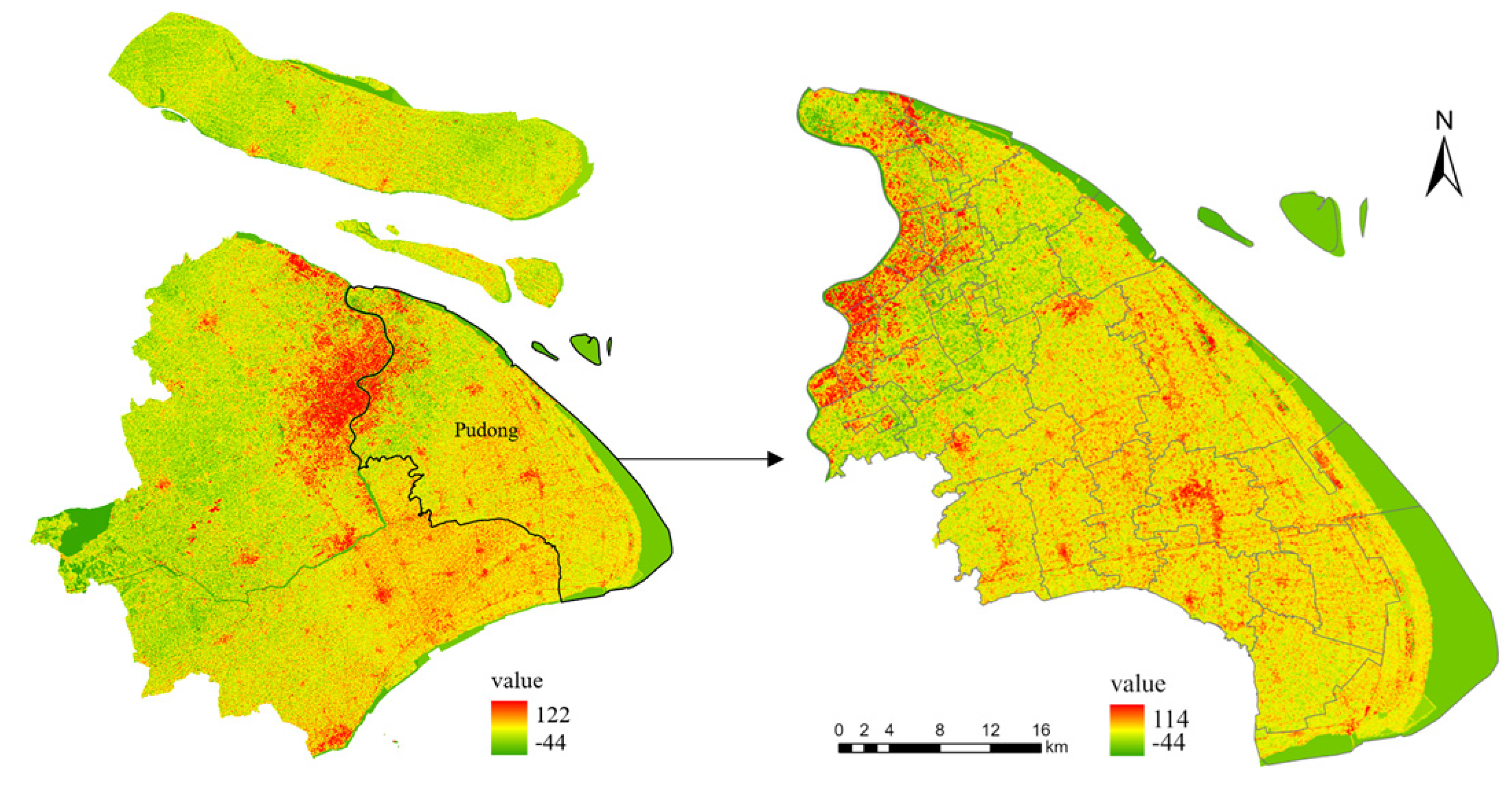
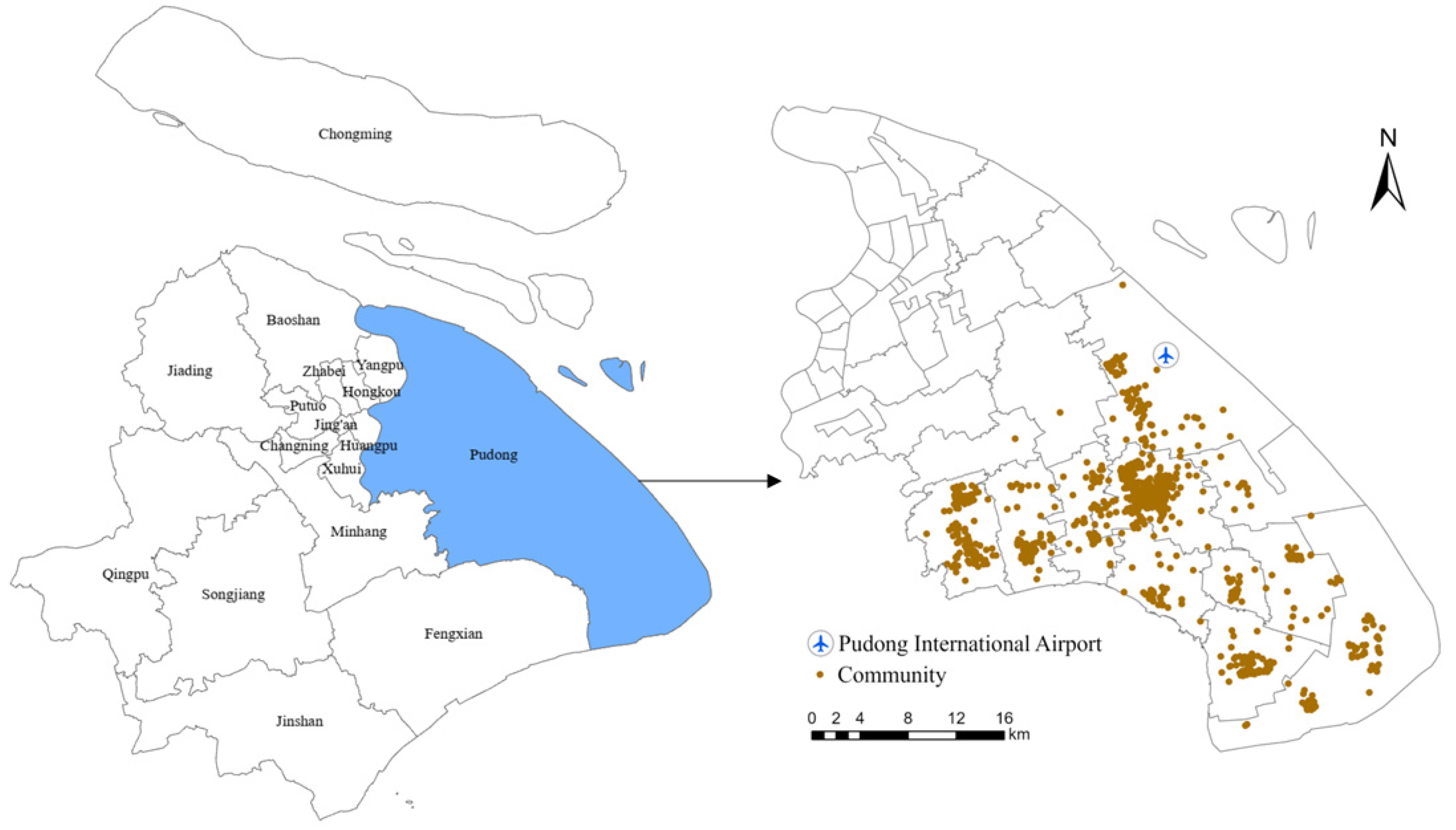
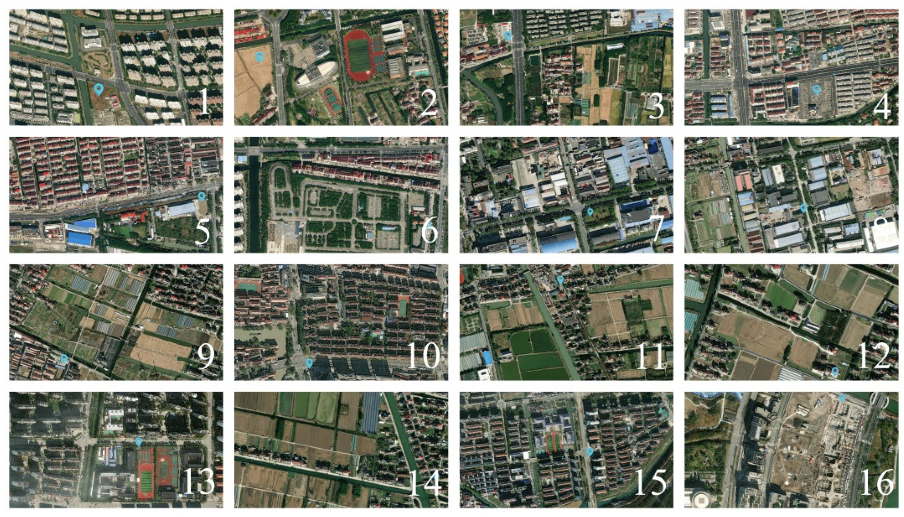
4. Data Collection
5. Case Study
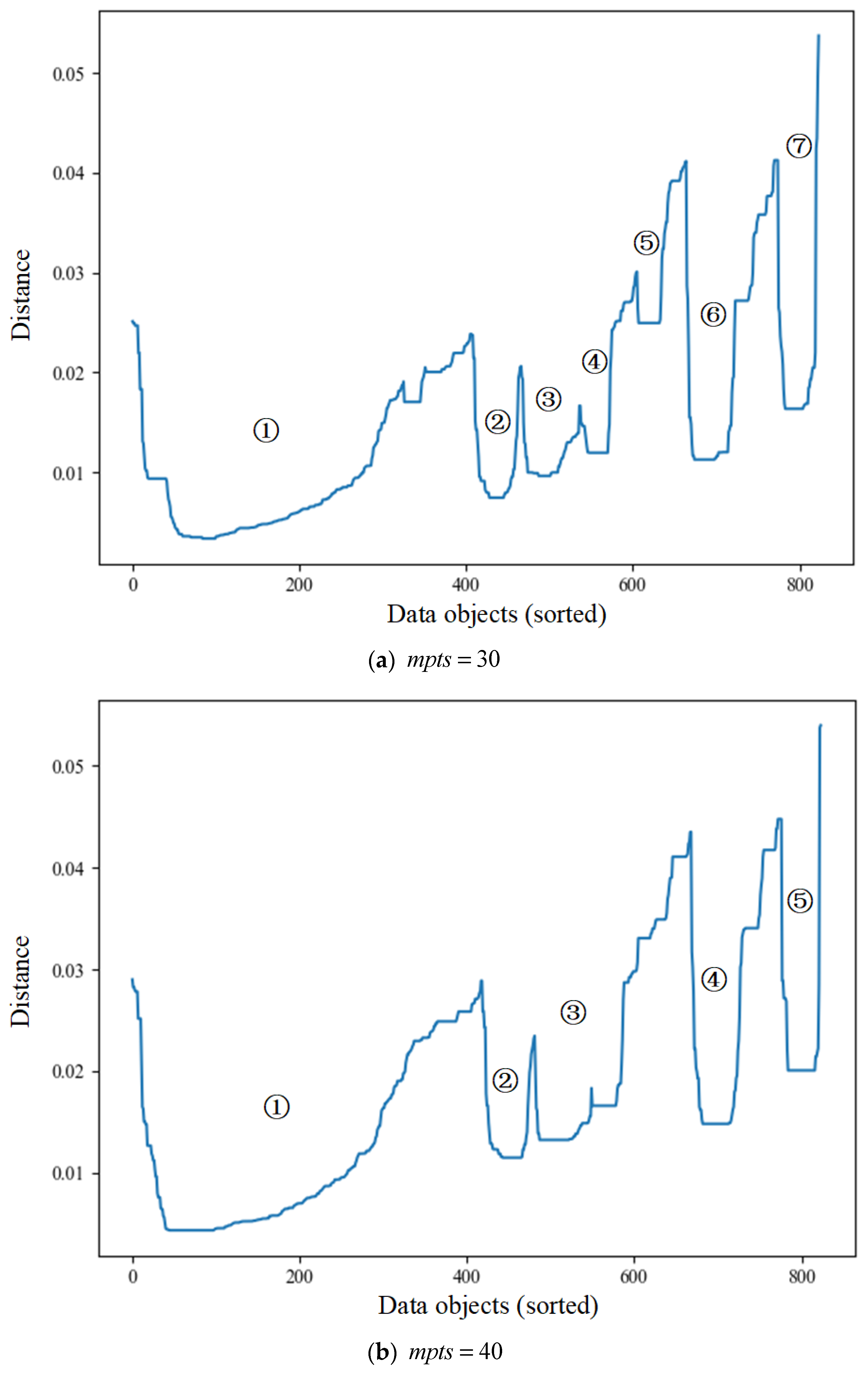
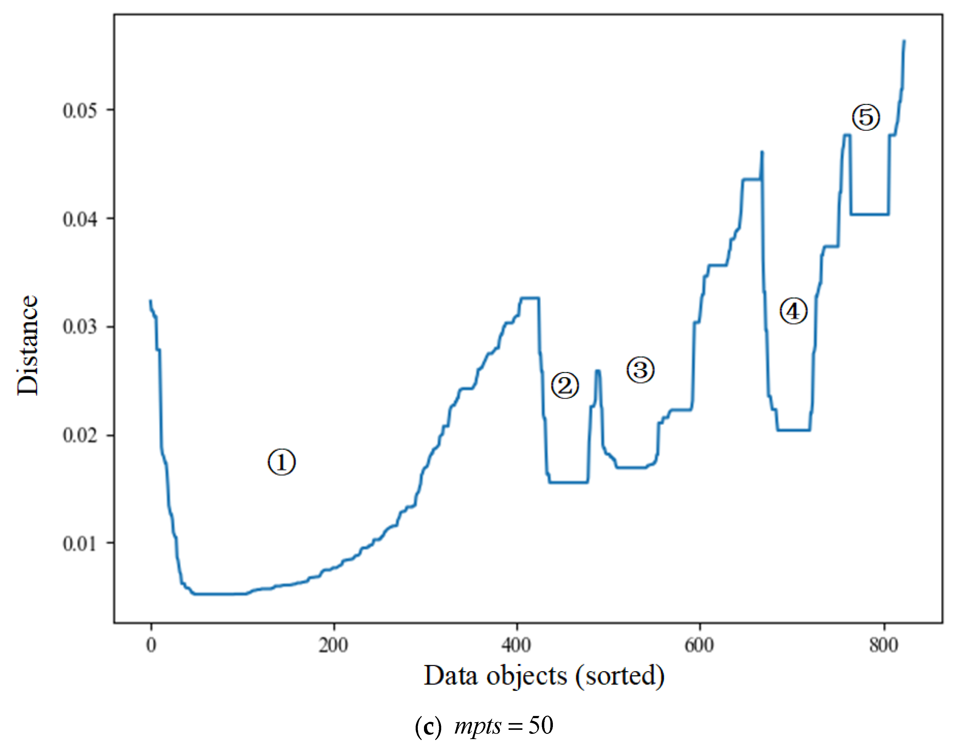
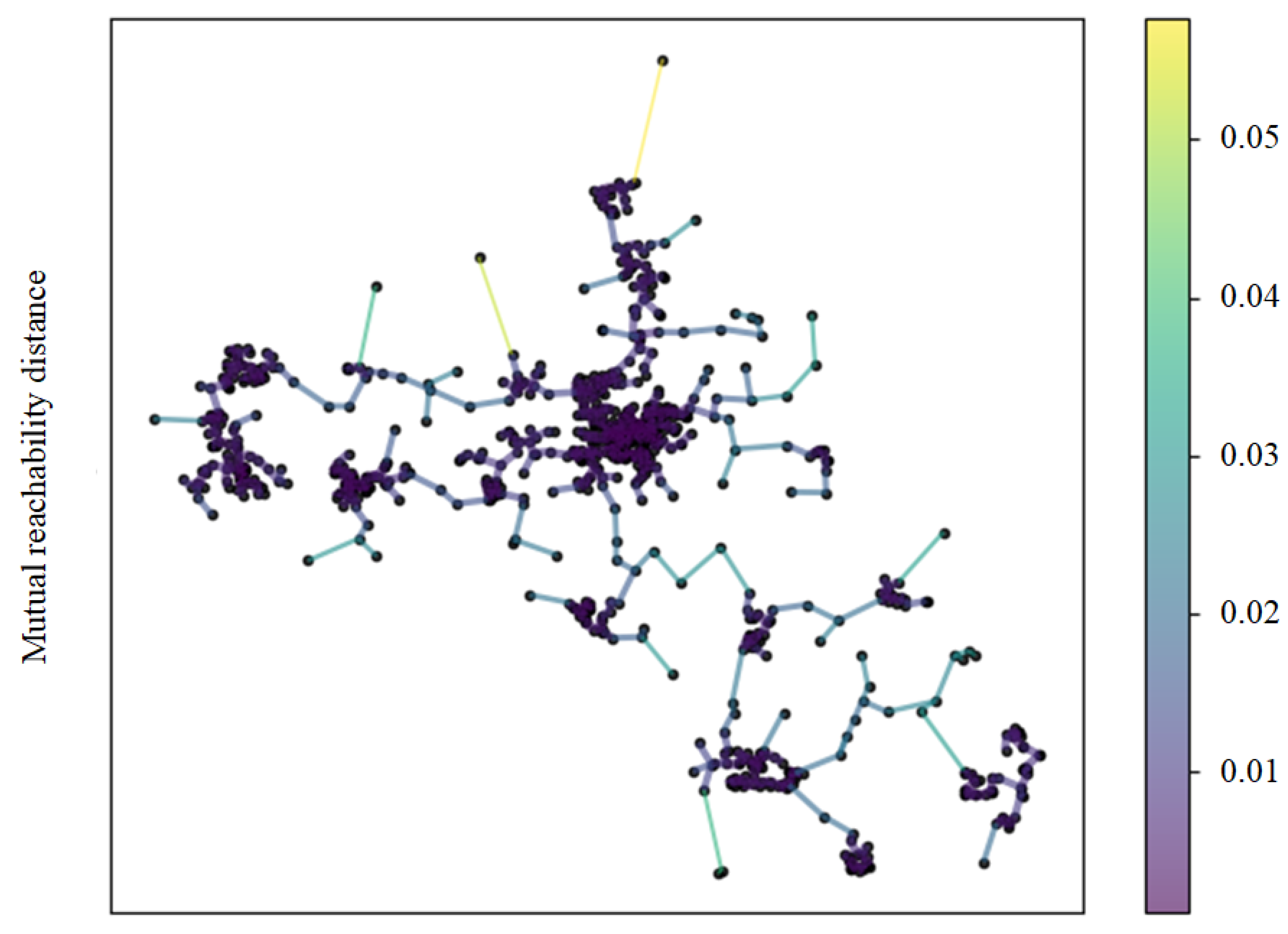
5.1. Accessibility Distance Analysis of OPTICS under Different mpts
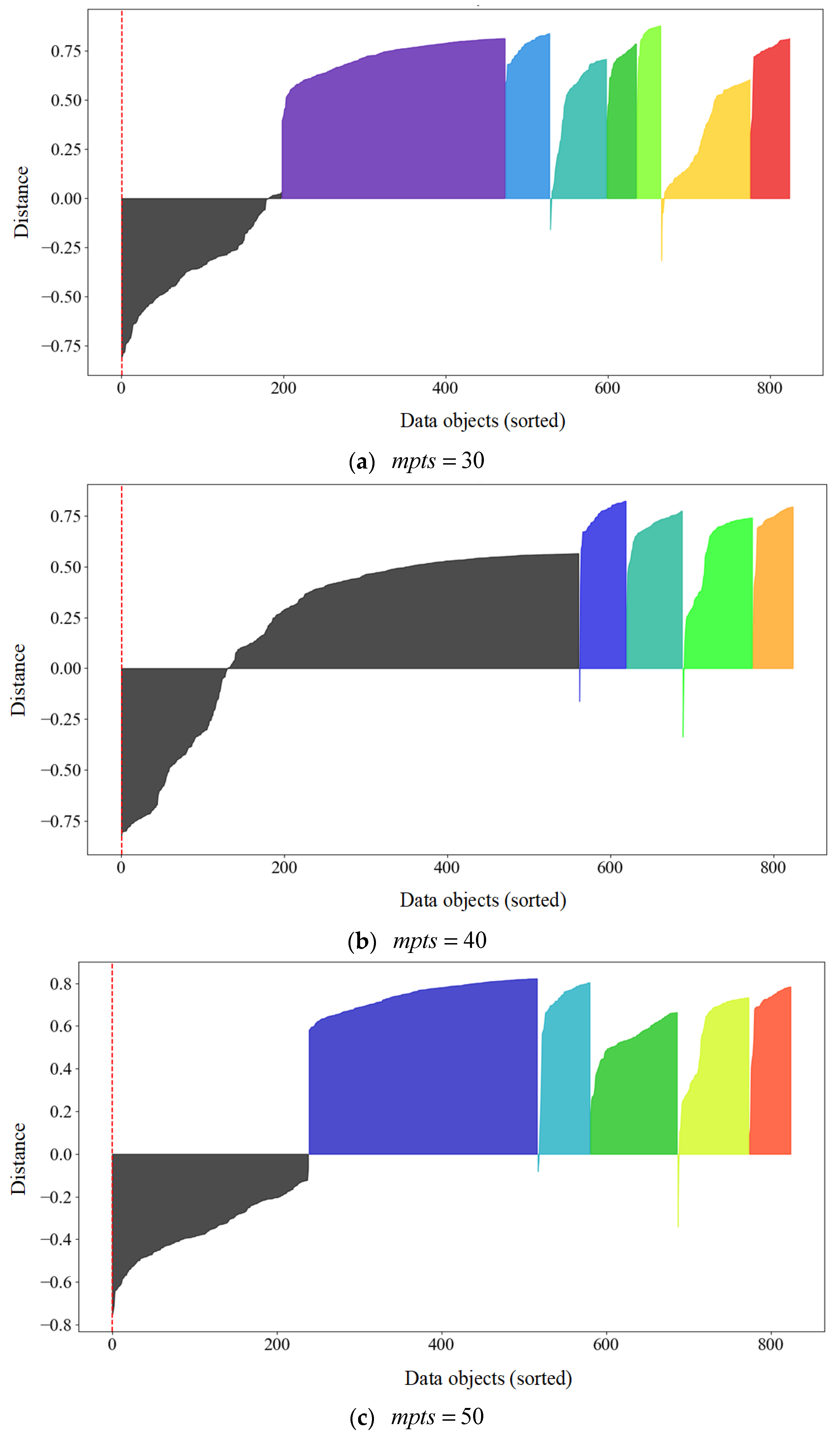
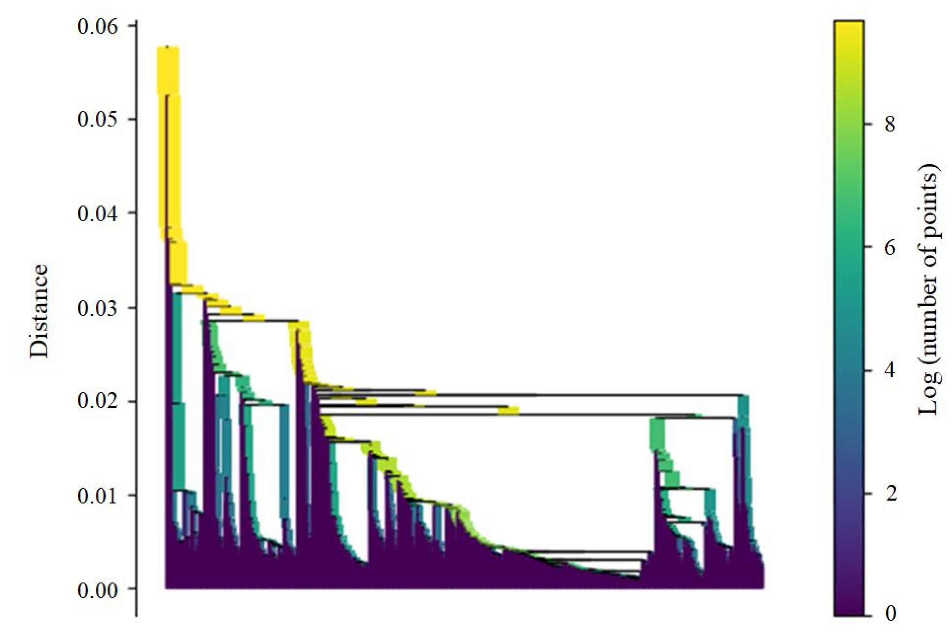
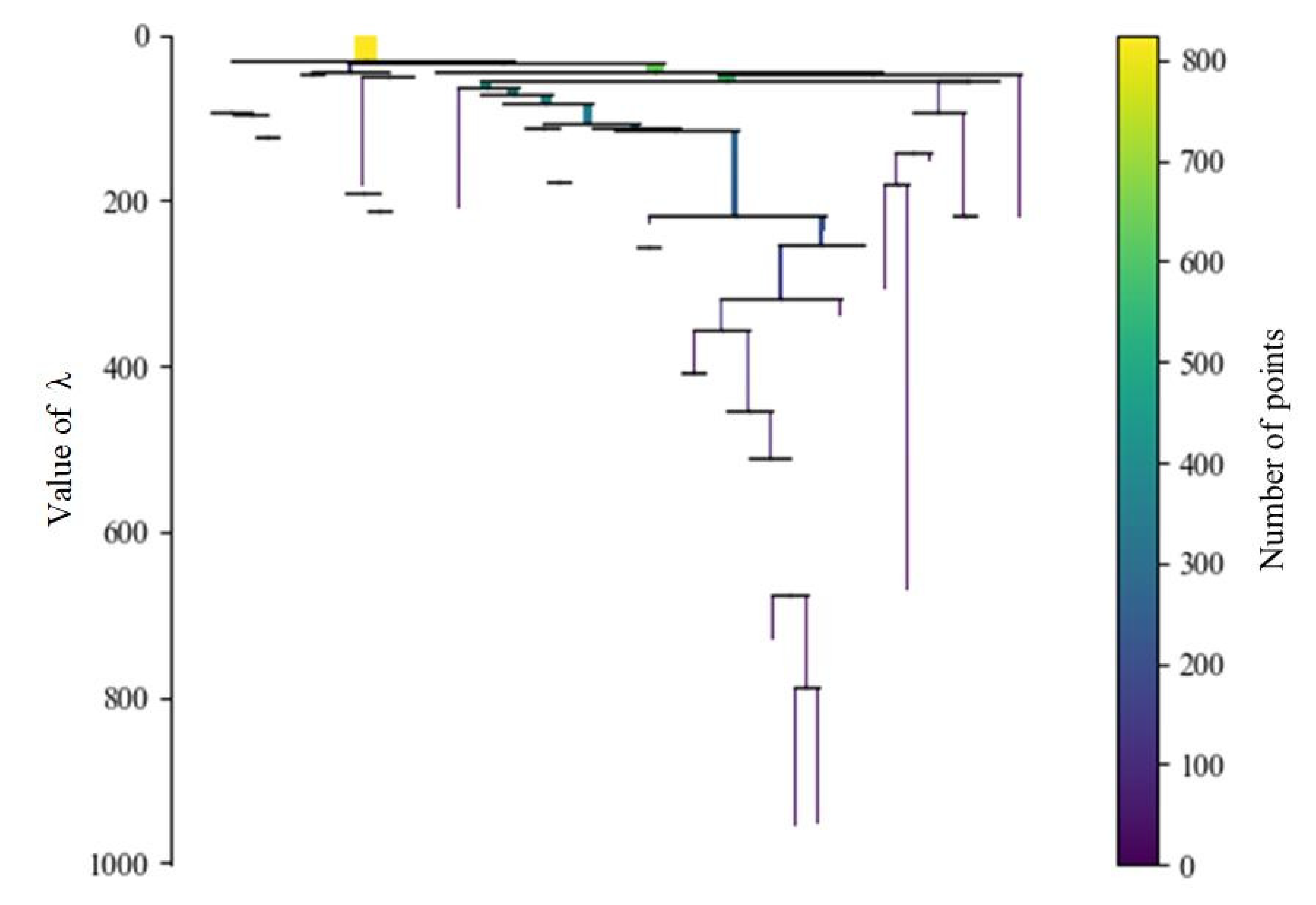
5.2. MST, Cluster Hierarchy and Extraction of Important Clusters
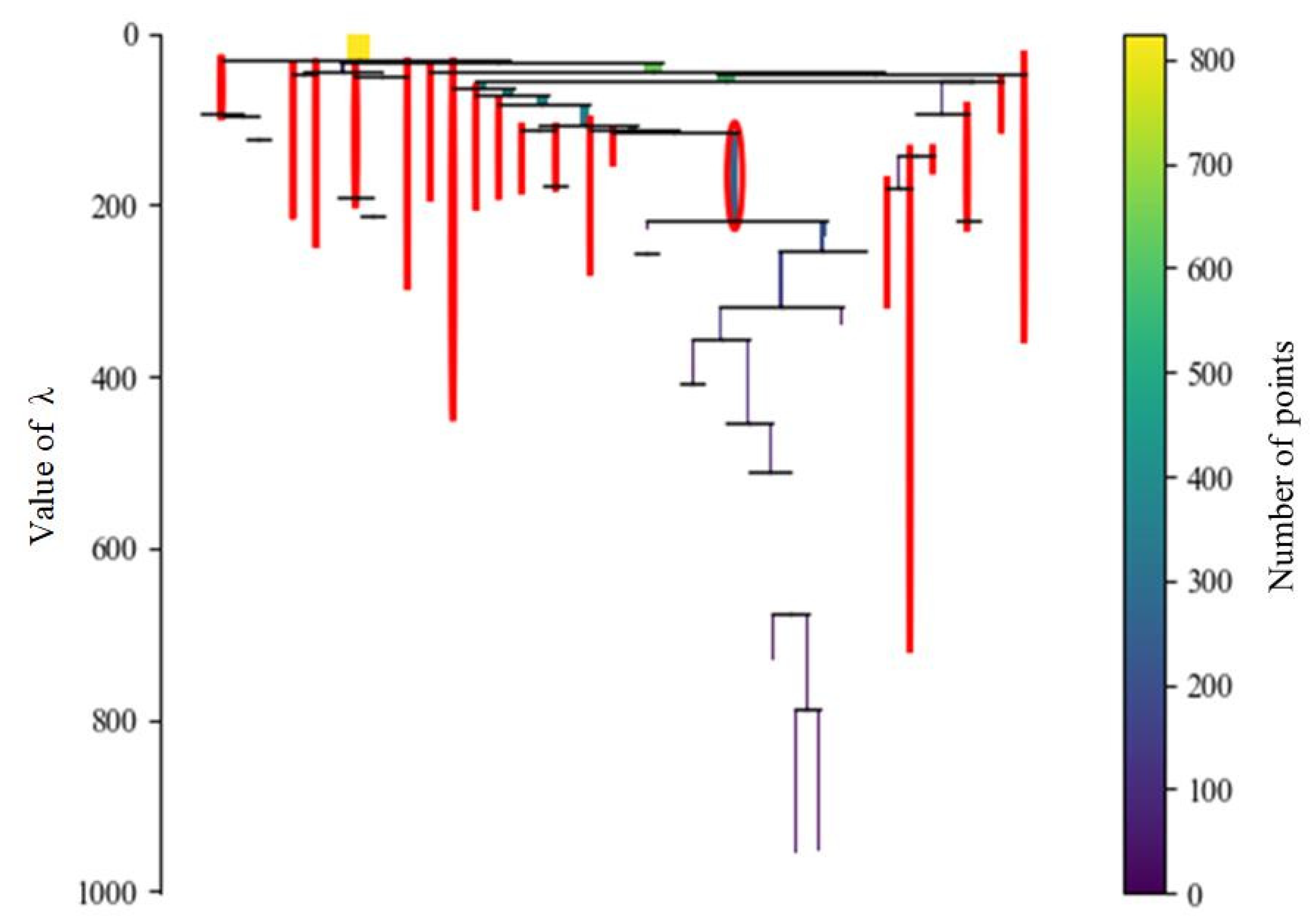
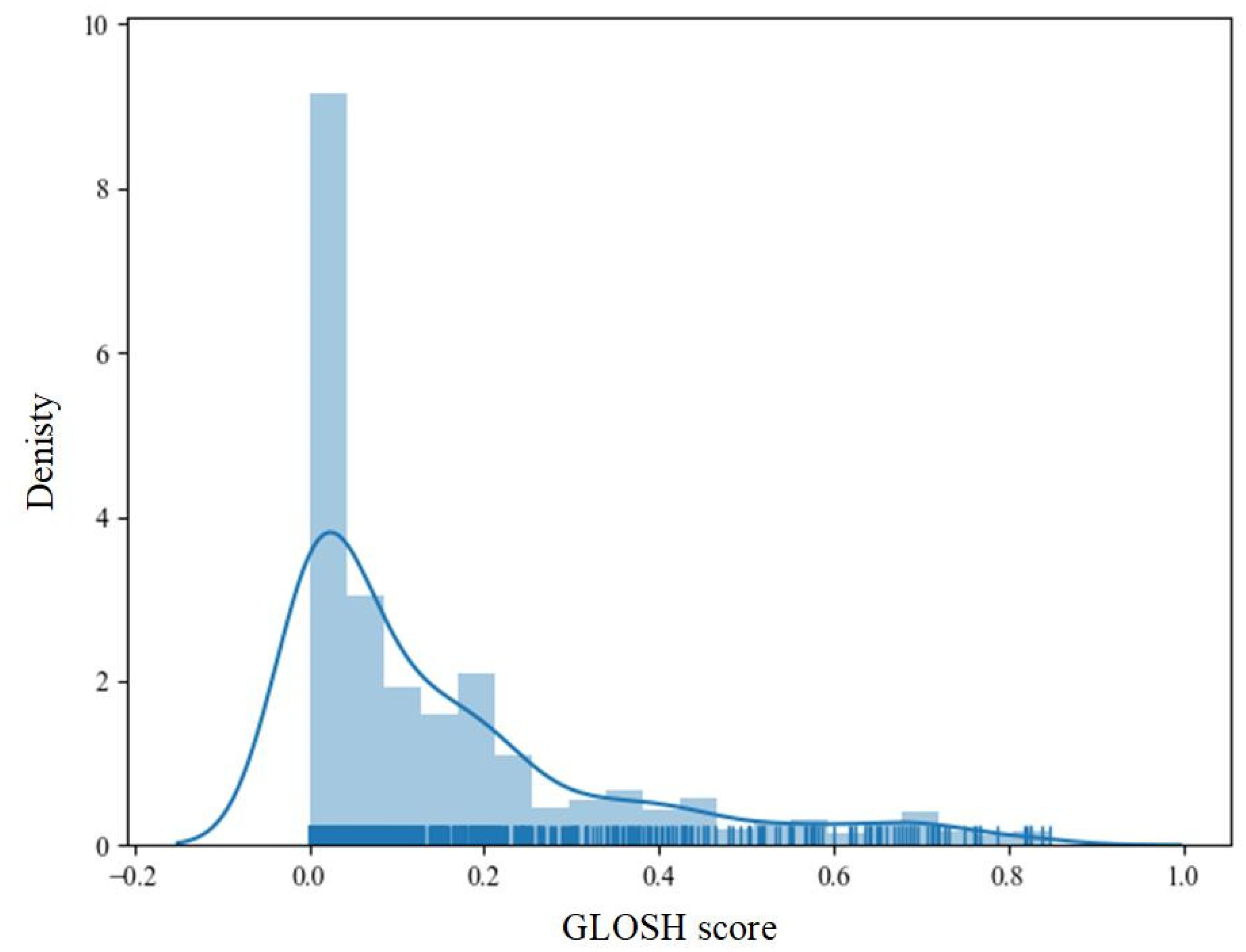
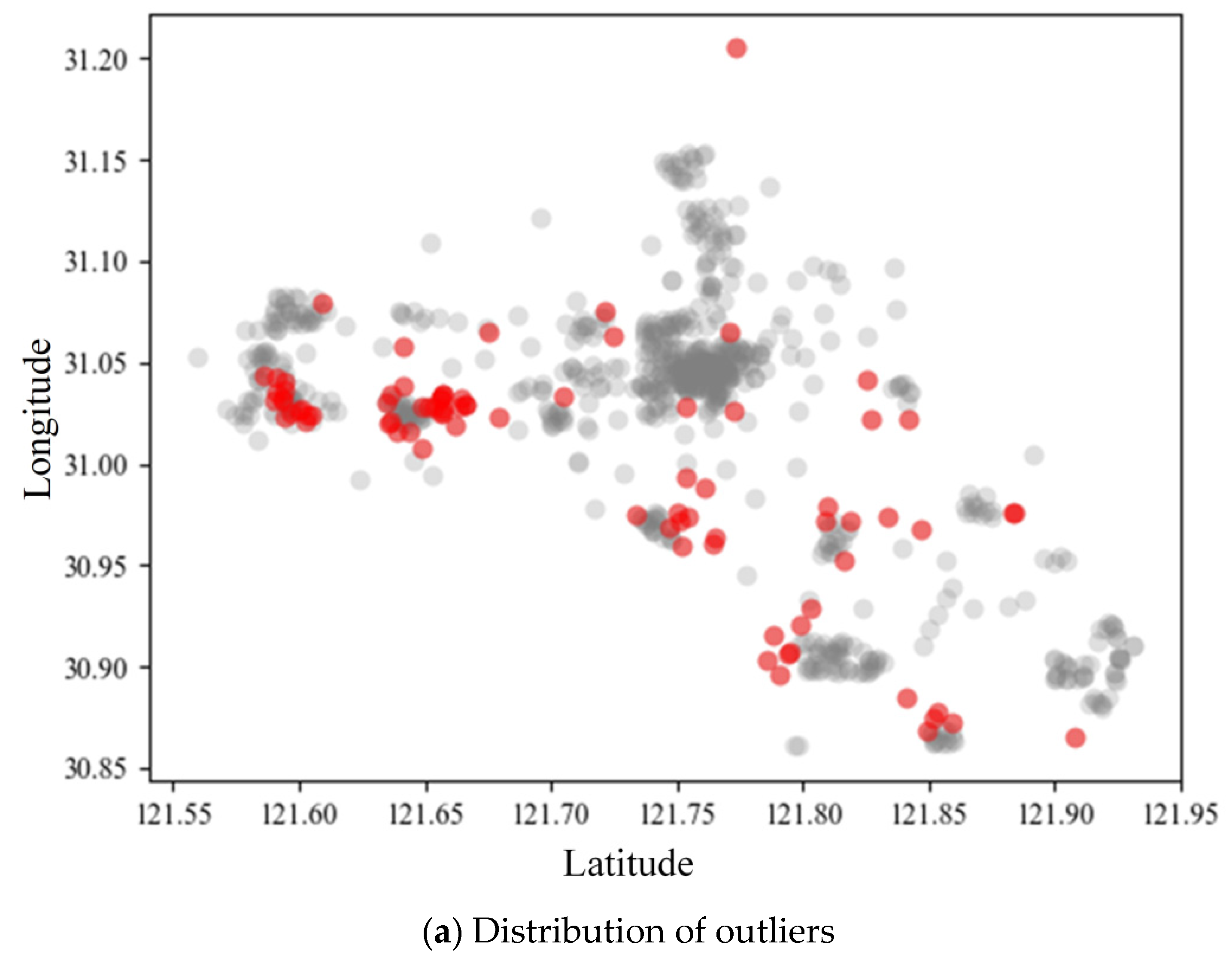
5.3. Outlier Monitoring of GLOSH
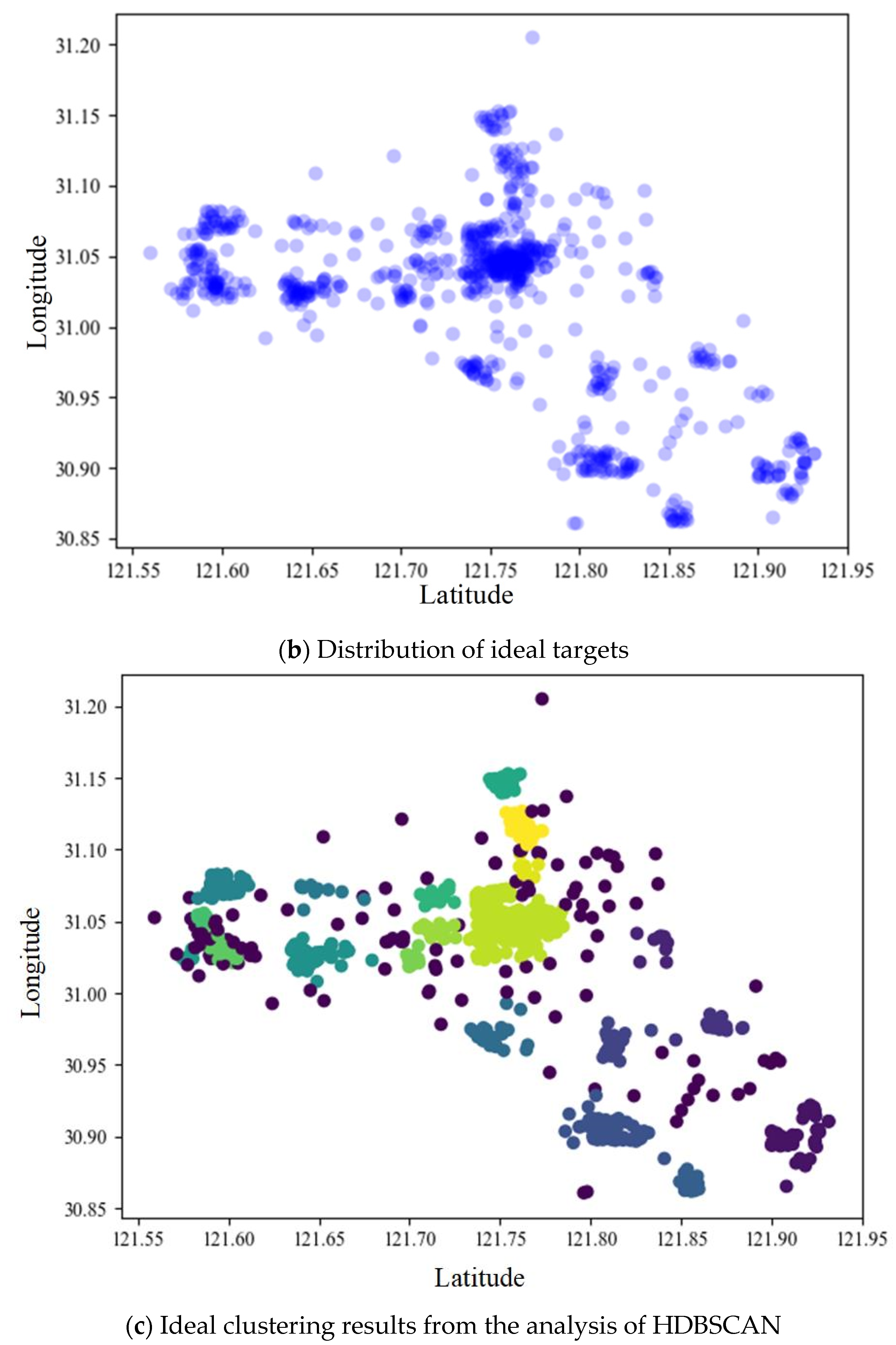
5.4. Determination and Correction of Ideal Points in Stations
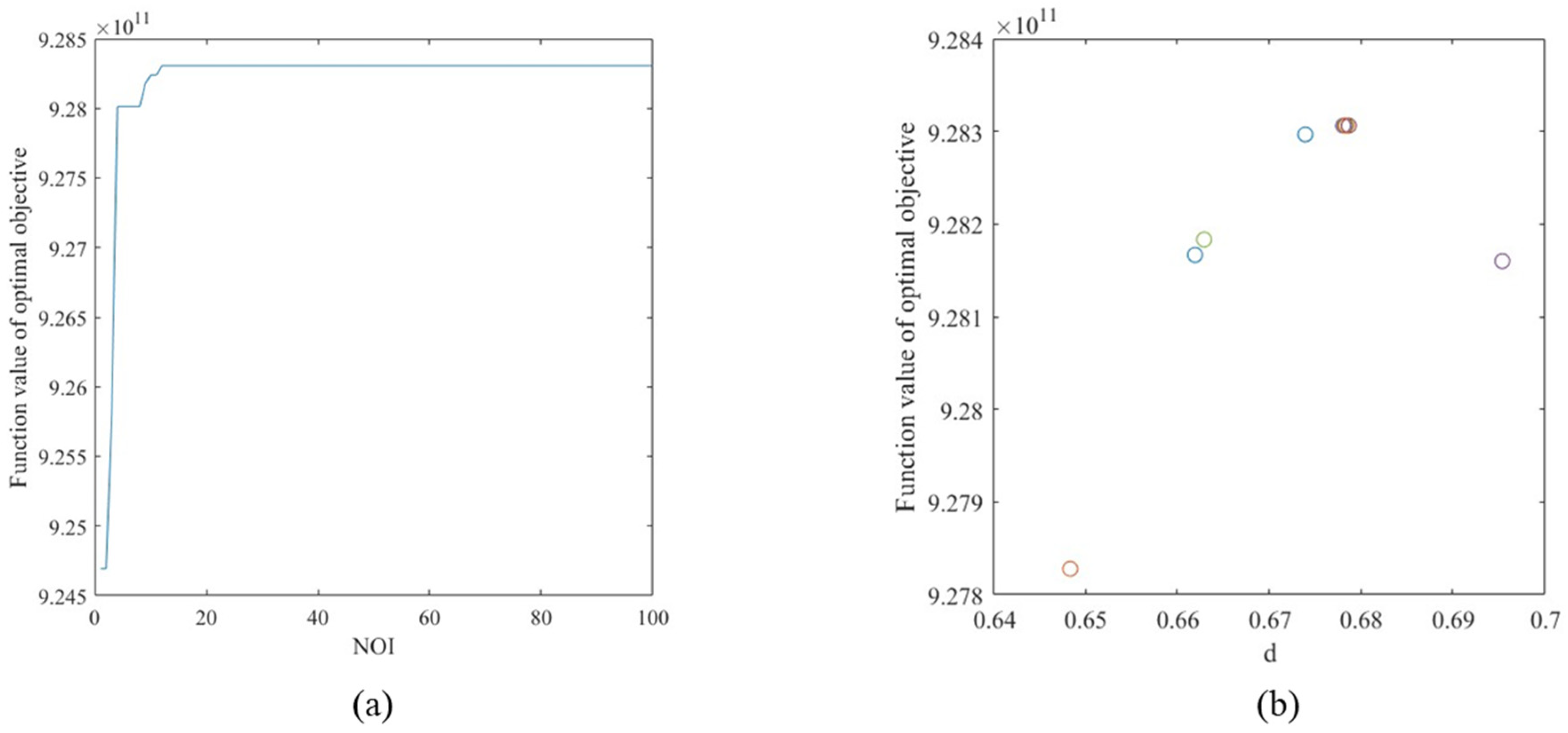
5.5. Analysis of Optimal Station Spacing
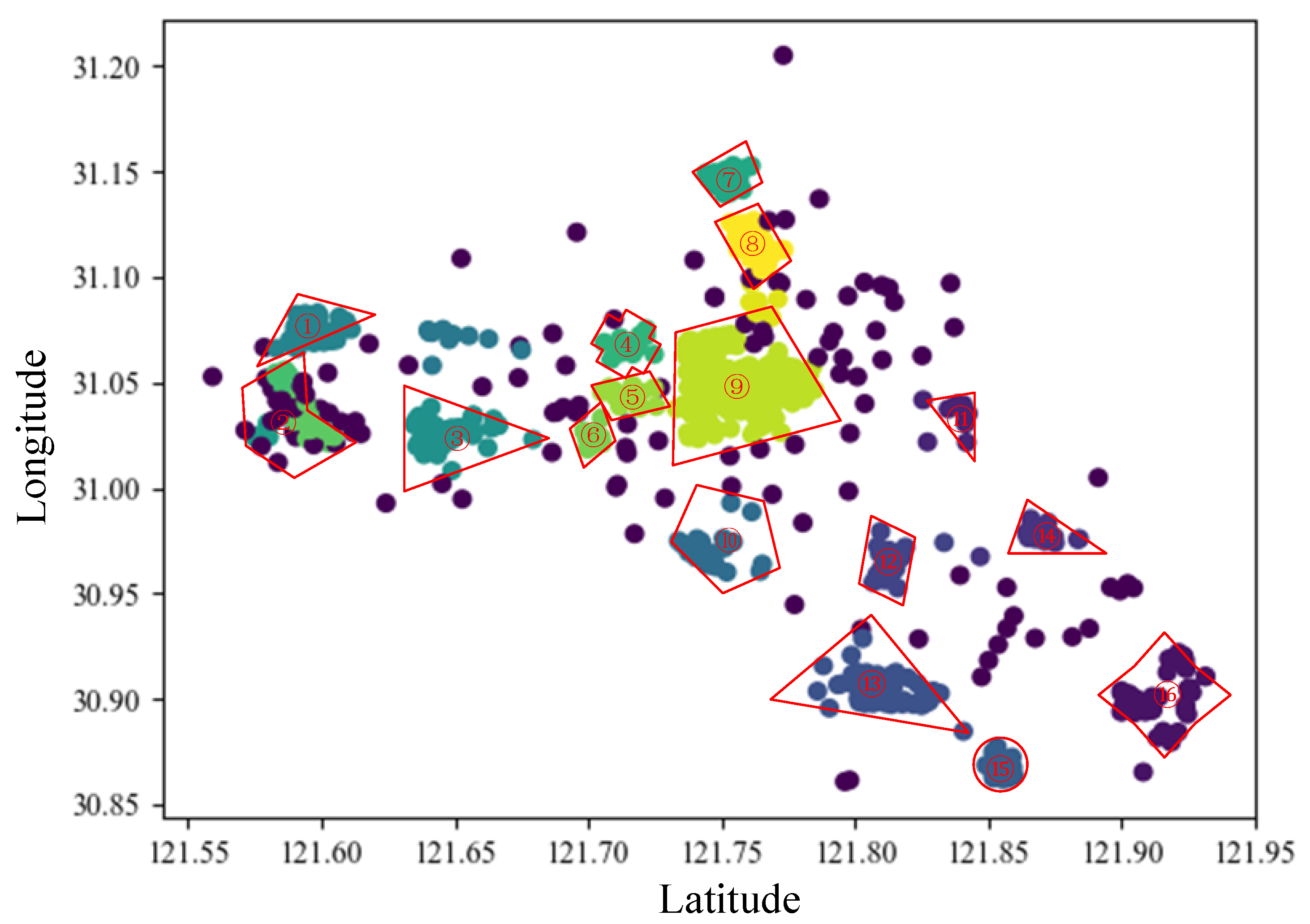
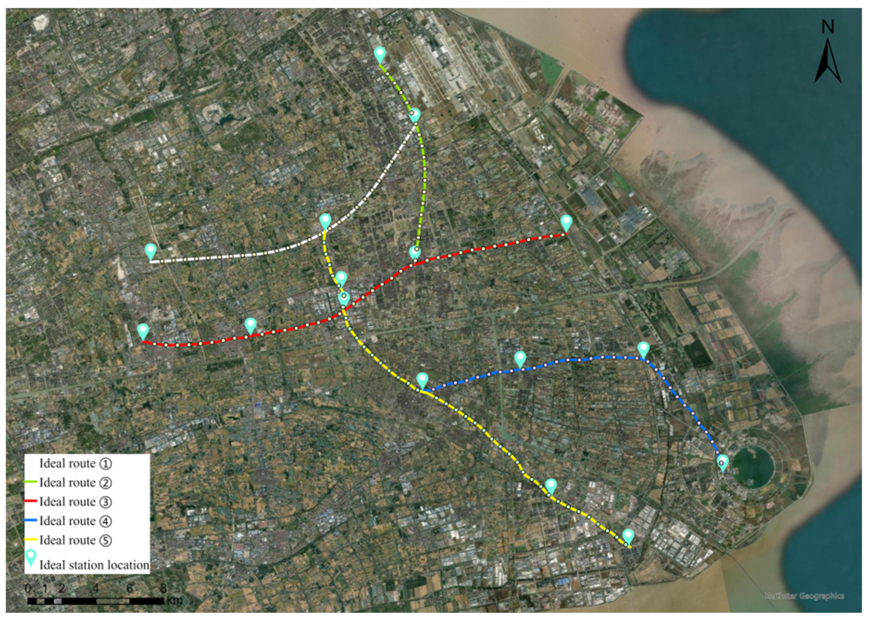
5.6. Determination of Metro Lines
6. Comparative Analysis with DBSCAN and K-Means Clustering Results
6.1. Time Complexity
6.2. Space Complexity
6.3. Silhouette Coefficient
6.4. Cluster View
7. Conclusions
Author Contributions
Funding
Institutional Review Board Statement
Informed Consent Statement
Data Availability Statement
Conflicts of Interest
References
- Cheng, J.; Yin, P. Analysis of the Complex Network of the Urban Function under the Lockdown of COVID-19: Evidence from Shenzhen in China. Mathematics 2022, 10, 2412. [Google Scholar] [CrossRef]
- Li, S.; Zhou, Y.; Kundu, T.; Sheu, J.B. Spatiotemporal variation of the worldwide air transportation network induced by COVID-19 pandemic in 2020. Transp. Policy 2021, 111, 168–184. [Google Scholar] [CrossRef] [PubMed]
- Liu, M.B.; Liao, S.M. A case study on the underground rapid transport system (URTS) for the international airport hubs: Planning, application and lessons learnt. Tunn. Undergr. Space Technol. 2018, 80, 114–122. [Google Scholar] [CrossRef]
- Cheng, J.; Xie, Y.; Zhang, J. Industry structure optimization via the complex network of industry space: A case study of Jiangxi Province in China. J. Clean. Prod. 2022, 338, 130602. [Google Scholar] [CrossRef]
- Mohaymany, A.S.; Gholami, A. Multimodal feeder network design problem: Ant colony optimization approach. J. Transp. Eng. 2010, 136, 323–331. [Google Scholar] [CrossRef]
- Lai, X. Optimization of Station Locations and Track Alignments for Rail Transit Lines; UMI: London, UK, 2012; pp. 87–120. [Google Scholar]
- Saidi, S.; Wirasinghe, S.C.; Kattan, L. Long-term planning for ring-radial urban rail transit networks. Transp. Res. Part B Methodol. 2016, 86, 128–146. [Google Scholar] [CrossRef]
- Lv, Z.; He, D.; Jia, H.F.; Li, C.B. Research on the Layout of the Integrative Urban Rail Transit Line Station; Trans Tech Publications Ltd.: Zurich, Switzerland, 2013; pp. 1222–1229. [Google Scholar]
- Chai, S.; Liang, Q.; Zhong, S. Design of urban rail transit network constrained by urban road network, trips and land-use characteristics. Sustainability 2019, 11, 6128. [Google Scholar] [CrossRef] [Green Version]
- Xu, H.; Qiu, Z.; Yuan, H. Research on the Location of Urban Rail Transit Station based on the Integration of Land Use Layout and Regional Transportation Network. In Proceedings of the 2021 6th International Conference on Transportation Information and Safety (ICTIS), Wuhan, China, 22–24 October 2021. [Google Scholar]
- Xia, S.; Peng, D.; Meng, D.; Zhang, C.; Wang, G.; Giem, E.; Chen, Z. A fast adaptive k-means with no bounds. IEEE Trans. Pattern Anal. Mach. Intell. 2020, 44, 87–99. [Google Scholar] [CrossRef]
- Jian, S.; Pang, G.; Cao, L.; Lu, K.; Gao, H. Cure: Flexible categorical data representation by hierarchical coupling learning. IEEE Trans. Knowl. Data Eng. 2018, 31, 853–866. [Google Scholar] [CrossRef]
- Yin, P.; Cheng, J.; Peng, M. Analyzing the Passenger Flow of Urban Rail Transit Stations by Using Entropy Weight-Grey Correlation Model: A Case Study of Shanghai in China. Mathematics 2022, 10, 3506. [Google Scholar] [CrossRef]
- Li, M.X.; Wang, X.Q. Data analysis of blast furnace gas center based on STING grid clustering. Mater. Sci. Eng. 2018, 439, 032017. [Google Scholar] [CrossRef]
- Khan, K.; Rehman, S.U.; Aziz, K.; Fong, S.; Sarasvady, S. DBSCAN: Past, present and future. In Proceedings of the Fifth International Conference on the Applications of Digital Information and Web Technologies (ICADIWT 2014), Bangalore, India, 17–19 February 2014. [Google Scholar]
- McInnes, L.; Healy, J.; Astels, S. hdbscan: Hierarchical density based clustering. J. Open Source Softw. 2017, 2, 205. [Google Scholar] [CrossRef]
- Melvin, R.L.; Xiao, J.; Godwin, R.C.; Berenhaut, K.S.; Salsbury, F.R. Visualizing correlated motion with HDBSCAN clustering. Protein Sci. 2018, 27, 62–75. [Google Scholar] [CrossRef] [PubMed] [Green Version]
- Ghamarian, I.; Marquis, E.A. Hierarchical density-based cluster analysis framework for atom probe tomography data. Ultramicroscopy 2019, 200, 28–38. [Google Scholar] [CrossRef]
- Wang, L.; Chen, P.; Chen, L.; Mou, J. Ship AIS trajectory clustering: An HDBSCAN-based approach. J. Mar. Sci. Eng. 2021, 9, 566. [Google Scholar] [CrossRef]
- Liu, P.; Yao, H.; Dai, H.; Fu, W. The Detection and Following of Human Legs Based on Feature Optimized HDBSCAN for Mobile Robot. J. Phys. 2022, 2216, 012009. [Google Scholar] [CrossRef]
- Givoni, M.; Chen, X. Airline and railway disintegration in China: The case of Shanghai Hongqiao Integrated Transport Hub. Transp. Lett. 2017, 9, 202–214. [Google Scholar] [CrossRef]
- Chang, Y.C. Factors affecting airport access mode choice for elderly air passengers. Transp. Res. Part E Logist. Transp. Rev. 2013, 57, 105–112. [Google Scholar] [CrossRef]
- Aqib, M.; Mehmood, R.; Alzahrani, A.; Katib, I.; Albeshri, A.; Altowaijri, S.M. Rapid transit systems: Smarter urban planning using big data, in-memory computing, deep learning, and GPUs. Sustainability 2019, 11, 2736. [Google Scholar] [CrossRef] [Green Version]
- Jiao, L.; Shen, L.; Shuai, C.; Tan, Y.; He, B. Measuring crowdedness between adjacent stations in an urban metro system: A chinese case study. Sustainability 2017, 9, 2325. [Google Scholar] [CrossRef] [Green Version]
- Wu, S.S.; Cheng, J.; Lo, S.M.; Chen, C.C.; Bai, Y. Coordinating urban construction and district-level population density for balanced development: An explorative structural equation modeling analysis on Shanghai. J. Clean. Prod. 2021, 312, 127646. [Google Scholar] [CrossRef]
- Caparros-Midwood, D.; Barr, S.; Dawson, R. Optimised spatial planning to meet long term urban sustainability objectives. Computers. Environ. Urban Syst. 2015, 54, 154–164. [Google Scholar] [CrossRef] [Green Version]
- Arbex, R.O.; da Cunha, C.B. Efficient transit network design and frequencies setting multi-objective optimization by alternating objective genetic algorithm. Transp. Res. Part B Methodol. 2015, 81, 355–376. [Google Scholar] [CrossRef]
- Liu, B.; Sun, S.; Mu, R. Performance Evaluation of Railway Logistics Based on the Layers of Entropy and Grey Correlation Degrees. In Proceedings of the International Conference of Logistics Engineering & Management, Shanghai, China, 9–11 October 2014. [Google Scholar]
- Zheng, J. The Relationship Between Property Value and Urban Rapid Rail Transit: Based on Improved Hedonic Price Model. Ph.D. Thesis, Tsinghua University, Beijing, China, 2004. [Google Scholar]
- Cheng, J. Analyzing the factors influencing the choice of the government on leasing different types of land uses: Evidence from Shanghai of China. Land Use Policy 2020, 90, 104303. [Google Scholar] [CrossRef]
- Cheng, J. Data analysis of the factors influencing the industrial land leasing in Shanghai based on mathematical models. Math. Probl. Eng. 2020, 2020, 1–11. [Google Scholar] [CrossRef] [Green Version]
- Lee, B.; Gordon, P.; Moore, J.E.; Richardson, H.W. The attributes of residence/workplace areas and transit commuting. J. Transp. Land Use 2011, 4, 43–63. [Google Scholar] [CrossRef]
- Cheng, J.; Xie, Y.; Zhang, J. Analyzing the Urban Hierarchical Structure Based on Multiple Indicators of Economy and Industry: An Econometric Study in China. CMES Comput. Model. Eng. Sci. 2022, 131, 1831–1855. [Google Scholar] [CrossRef]
- Cooper, C.H.; Harvey, I.; Orford, S.; Chiaradia, A.J. Using multiple hybrid spatial design network analysis to predict longitudinal effect of a major city centre redevelopment on pedestrian flows. Transportation 2021, 48, 643–672. [Google Scholar] [CrossRef] [Green Version]
- Qiang, H.; Hu, L. Population and capital flows in metropolitan Beijing, China: Empirical evidence from the past 30 years. Cities 2022, 120, 103464. [Google Scholar] [CrossRef]
- Zornoza-Gallego, C. Means of Transport and Population Distribution in Metropolitan Areas: An Evolutionary Analysis of the Valencia Metropolitan Area. Land 2022, 11, 657. [Google Scholar] [CrossRef]
- Cheng, J. Analysis of commercial land leasing of the district governments of Beijing in China. Land Use Policy 2021, 100, 104881. [Google Scholar] [CrossRef]
- Cheng, J. Residential land leasing and price under public land ownership. J. Urban Plan. Dev. 2021, 147, 05021009. [Google Scholar] [CrossRef]
- Cheng, J.; Luo, X. Analyzing the Land Leasing Behavior of the Government of Beijing, China, via the Multinomial Logit Model. Land 2022, 11, 376. [Google Scholar] [CrossRef]
- Cheng, J. Analysis of the factors influencing industrial land leasing in Beijing of China based on the district-level data. Land Use Policy 2022, 122, 106389. [Google Scholar] [CrossRef]
- Caros, N.S.; Guo, X.; Stewart, A.; Attanucci, J.; Smith, N.; Nioras, D.; Zimmer, A. Ridership and Operations Visualization Engine: An Integrated Transit Performance and Passenger Journey Visualization Engine. Transp. Res. Rec. 2023, 2677, 1082–1097. [Google Scholar] [CrossRef]
- Cheng, J. Mathematical models and data analysis of residential land leasing behavior of district governments of Beijing in China. Mathematics 2021, 9, 2314. [Google Scholar] [CrossRef]
- Zou, Y.; Wang, L.; Xue, Z.; Jiang, M.; Lu, X.; Yang, S.; Yu, X. Impacts of agricultural and reclamation practices on wetlands in the Amur River Basin, Northeastern China. Wetlands 2018, 38, 383–389. [Google Scholar] [CrossRef]
- Susilo, Y.O.; Dijst, M. How Far is Too Far? Travel time ratios for activity participation in the Netherlands. Transp. Res. Rec. 2009, 2134, 89–98. [Google Scholar] [CrossRef]
- Yiu, C.Y.; Wong, S.K. The effects of expected transport improvements on housing prices. Urban Stud. 2005, 42, 113–125. [Google Scholar] [CrossRef]
- Campello, R.J.; Moulavi, D.; Sander, J. Density-based clustering based on hierarchical density estimates. In Proceedings of the Advances in Knowledge Discovery and Data Mining: 17th Pacific-Asia Conference, Gold Coast, Australia, 14–17 April 2013. [Google Scholar]
- Ko, K.; Cao, X.J. The impact of Hiawatha Light Rail on commercial and industrial property values in Minneapolis. J. Public Transp. 2013, 16, 47–66. [Google Scholar] [CrossRef] [Green Version]
- Yin, P.; Cheng, J. A MySQL-based software system of urban land planning database of Shanghai in China. CMES Comput. Model. Eng. Sci. 2023, 135, 2387–2405. [Google Scholar] [CrossRef]
- Dette, H.; Wu, W. Detecting relevant changes in the mean of nonstationary processes—A mass excess approach. Ann. Stat. 2019, 47, 3578–3608. [Google Scholar] [CrossRef]
- Basora, L.; Olive, X.; Dubot, T. Recent advances in anomaly detection methods applied to aviation. Aerospace 2019, 6, 117. [Google Scholar] [CrossRef] [Green Version]
- Zheng, S.; Kahn, M.E. Land and residential property markets in a booming economy: New evidence from Beijing. J. Urban Econ. 2008, 63, 743–757. [Google Scholar] [CrossRef]
- Graham, D.J.; Carbo, J.M.; Anderson, R.J.; Bansal, P. Understanding the costs of urban rail transport operations. Transp. Res. Part B Methodol. 2020, 138, 292–316. [Google Scholar]
- Sun, Y.; Shi, J.; Schonfeld, P.M. Identifying passenger flow characteristics and evaluating travel time reliability by visualizing AFC data: A case study of Shanghai Metro. Public Transp. 2016, 8, 341–363. [Google Scholar] [CrossRef]
- González-Gil, A.; Palacin, R.; Batty, P.; Powell, J.P. A systems approach to reduce urban rail energy consumption. Energy Convers. Manag. 2014, 80, 509–524. [Google Scholar] [CrossRef] [Green Version]
- Guo, S.; Yu, L.; Chen, X.; Zhang, Y. Modelling waiting time for passengers transferring from rail to buses. Transp. Plan. Technol. 2011, 34, 795–809. [Google Scholar] [CrossRef]
- Cai, J.; Wei, H.; Yang, H.; Zhao, X. A novel clustering algorithm based on DPC and PSO. IEEE Access 2020, 8, 88200–88214. [Google Scholar] [CrossRef]
- Kifana, B.D.; Abdurohman, M. Great circle distance methode for improving operational control system based on gps tracking system. Int. J. Comput. Sci. Eng. 2012, 4, 647. [Google Scholar]
- Marini, F.; Walczak, B. Particle swarm optimization (PSO). A tutorial. Chemom. Intell. Lab. Syst. 2015, 149, 153–165. [Google Scholar] [CrossRef]
- Pakhira, M.K. A linear time-complexity k-means algorithm using cluster shifting. In Proceedings of the 2014 international conference on computational intelligence and communication networks, Bhopal, India, 14–16 November 2014. [Google Scholar]
- Arora, P.; Varshney, S. Analysis of k-means and k-medoids algorithm for big data. Procedia Comput. Sci. 2016, 78, 507–512. [Google Scholar] [CrossRef] [Green Version]
- Dinh, D.T.; Fujinami, T.; Huynh, V.N. Estimating the optimal number of clusters in categorical data clustering by silhouette coefficient. In Proceedings of the Knowledge and Systems Sciences: 20th International Symposium, Da Nang, Vietnam, 29 November 2019. [Google Scholar]


| Township | Types of Building | Types of Properties | ||||||
|---|---|---|---|---|---|---|---|---|
| Mid Rise | Mid-High Rise | High Rise | Residential Building | Factory Building | Office Building | House -Holds | SPR (CNY) | |
| Huinan | 98 | 14 | 35 | 97 | 27 | 23 | 78,908 | 26,480 |
| Xinchang | 61 | 4 | 15 | 58 | 16 | 6 | 48,915 | 27,832 |
| Datuan | 48 | 8 | 12 | 53 | 10 | 5 | 60,650 | 18,612 |
| Hangtou | 70 | 7 | 31 | 76 | 15 | 17 | 60,870 | 33,052 |
| Zhuqiao | 50 | 7 | 8 | 42 | 20 | 3 | 69,960 | 29,940 |
| Nicheng | 52 | 13 | 14 | 62 | 13 | 4 | 42,120 | 20,303 |
| Xuanqiao | 37 | 8 | 8 | 21 | 25 | 7 | 34,254 | 22,489 |
| Shuyuan | 32 | 2 | 6 | 35 | 4 | 1 | 30,318 | 18,052 |
| Wanxiang | 31 | 6 | 4 | 32 | 8 | 1 | 21,231 | 18,844 |
| Laogang | 33 | 5 | 0 | 31 | 7 | 0 | 11,030 | 17,576 |
| Nanhui New Town | 65 | 19 | 22 | 91 | 7 | 8 | 79,176 | 33,748 |
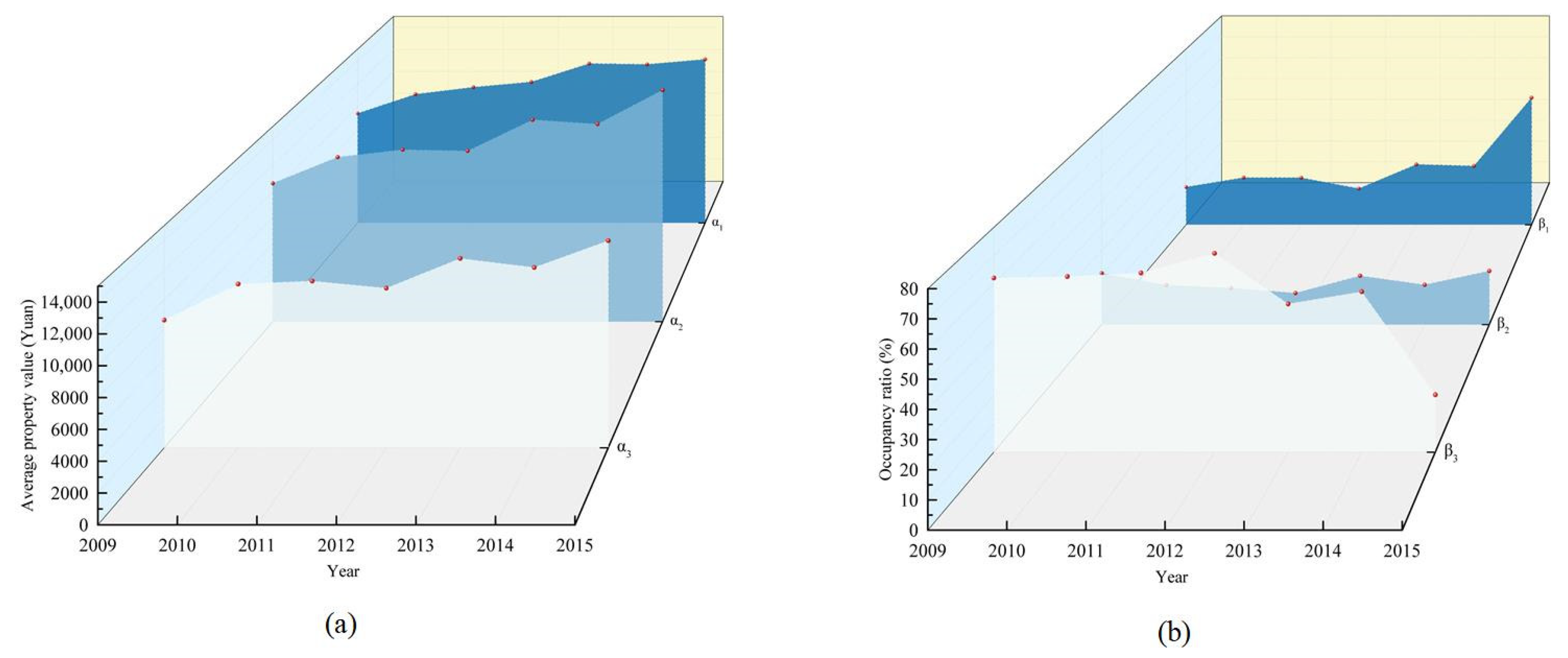
| Year | c1 | β1 | θ1 | c2 | β2 | θ2 | c3 | β3 | θ3 |
|---|---|---|---|---|---|---|---|---|---|
| 2009 | 1579.49 | 17.16% | 1.59 | 2014.65 | 20.84% | 1.97 | 2036.41 | 62.00% | 1.54 |
| 2010 | 1658.32 | 21.47% | 1.61 | 12651.34 | 16.01% | 2.13 | 2436.73 | 62.52% | 1.54 |
| 2011 | 608.03 | 21.39% | 1.80 | 570.63 | 14.82% | 2.38 | 199.38 | 63.79% | 1.56 |
| 2012 | 452.28 | 16.46% | 1.81 | −93.72 | 12.77% | 2.31 | −480.51 | 70.77% | 1.63 |
| 2013 | 1587.46 | 27.47% | 1.89 | 2391.55 | 19.77% | 2.51 | 2007.78 | 52.76% | 1.70 |
| 2014 | −69.8 | 26.75% | 1.87 | −323.21 | 16.13% | 2.07 | −612.38 | 57.12% | 1.54 |
| 2015 | 433.07 | 57.82% | 1.88 | 2610.45 | 21.75% | 2.64 | 1810.64 | 20.43% | 1.51 |
| Algorithm | Time Complexity | Space Complexity | Silhouette Coefficient | Number of Clusters |
|---|---|---|---|---|
| DBSCAN | O(68025) | O(825) | 0.3378 | 8 |
| K-means | O(37125) | O(1668) | 0.5488 | 9 |
| HDBSCAN | O(68025) | O(825) | 0.6043 | 16 |
Disclaimer/Publisher’s Note: The statements, opinions and data contained in all publications are solely those of the individual author(s) and contributor(s) and not of MDPI and/or the editor(s). MDPI and/or the editor(s) disclaim responsibility for any injury to people or property resulting from any ideas, methods, instructions or products referred to in the content. |
© 2023 by the authors. Licensee MDPI, Basel, Switzerland. This article is an open access article distributed under the terms and conditions of the Creative Commons Attribution (CC BY) license (https://creativecommons.org/licenses/by/4.0/).
Share and Cite
Yin, P.; Peng, M. Station Layout Optimization and Route Selection of Urban Rail Transit Planning: A Case Study of Shanghai Pudong International Airport. Mathematics 2023, 11, 1539. https://doi.org/10.3390/math11061539
Yin P, Peng M. Station Layout Optimization and Route Selection of Urban Rail Transit Planning: A Case Study of Shanghai Pudong International Airport. Mathematics. 2023; 11(6):1539. https://doi.org/10.3390/math11061539
Chicago/Turabian StyleYin, Pei, and Miaojuan Peng. 2023. "Station Layout Optimization and Route Selection of Urban Rail Transit Planning: A Case Study of Shanghai Pudong International Airport" Mathematics 11, no. 6: 1539. https://doi.org/10.3390/math11061539