Article

The Novel Analytical–Numerical Method for Multi-Dimensional Multi-Term Time-Fractional Equations with General Boundary Conditions

1
College of Mechanics and Materials, Hohai University, Nanjing 210098, China
2
A. Pidhornyi Institute of Mechanical Engineering Problems of NAS of Ukraine, 2/10 Pozharsky Street, 61046 Kharkiv, Ukraine
3
Nanjing Hydraulic Research Institute, Nanjing 210029, China
*
Author to whom correspondence should be addressed.
These authors contributed equally to this work.
Mathematics 2023, 11(4), 929; https://doi.org/10.3390/math11040929
Submission received: 5 January 2023 / Revised: 7 February 2023 / Accepted: 10 February 2023 / Published: 12 February 2023
(This article belongs to the Special Issue Computational Methods and Applications for Numerical Analysis)

Abstract

:
This article presents a simple but effective two-step analytical–numerical algorithm for solving multi-dimensional multi-term time-fractional equations. The first step is to derive an analytic representation that satisfies boundary requirements for 1D, 2D, and 3D problems, respectively. The second step is the meshless approximation where the Müntz polynomials are used to form the approximate solution and the unknown parameters are obtained by imposing the approximation for the governing equations. We illustrate first the detailed derivation of the analytic approximation and then the numerical implementation of the solution procedure. Several numerical examples are provided to verify the accuracy, efficiency, and adaptability to problems with general boundary conditions. The numerical results are compared with exact solutions and numerical methods reported in the literature, showing that the algorithm has great potential for multi-dimensional multi-term time-fractional equations with various boundary conditions.

1. Introduction

In recent years, many mathematical models with time-fractional multi-term derivatives have been studied in physics, hydrology, chemistry, etc. Hilfer [1] provided a collection of fractional calculus applications in physics. Molz [2] reviewed some fundamental properties of fractional motion and applications in hydrology. Singh [3] analyzed a chemical kinetics system pertaining to a fractional derivative. Furthermore, the applications of fractional equations can also be found in [4]. The well-known cable equations with fractional-order temporal operators belong to this class. They were introduced to model electronic properties of spiny neuronal dendrites [5,6]. The time-fractional partial differential equations (TFPDEs) can also include the Sobolev equations, which have been used to model many phenomena, such as the migration of moisture in soil, thermodynamics, and the motion of fluid in various media [7,8]. The equations of different models of heat transfer, whether the classical or dual-phase-lagging ones, undoubtedly also fall into this group [9]. Fractional differential equations have broad applications for the fact that fractional operators can describe physical phenomena more precisely than classical integral operators for some practical problems. The collection of real world applications of fractional differential equations can be seen in [10] and references therein.
Solutions to fractional partial differential equations are crucial for representing physical phenomena. Some analytical methods have been proposed that can be useful for parametric study. Liu carried out an analytical study for magnetohydrodynamic flow using fractional derivatives [11]. Ming derived the analytical solution for the problems containing multi-term time-fractional diffusion [12]. Ding proposed an analytical solution to the multi-term TFPDEs considering the non-local damping term [13] and also the fractional delay PDEs with mixed boundary conditions [14]. Jong used the analytic expression of the multi-term fractional integral operators to obtain the analytical expressions for the fractional equations [15]. Jiang investigated the multi-term fractional diffusion equations and obtained the analytical solutions by the method of separation variables [16]. In [17], the Laplace transform method was used to derive the solution to the time-fractional distributed-order heat conduction law. The Adomian decomposition method was also being used in [18]. Despite the fact that so many analytical techniques have been developed, the explicit forms of analytical or semi-analytical solutions are rare only for some problems under certain idealized conditions. For the further prospects of engineering applications, the numerical methods are still necessary and useful tools in this field. Numerical methods have already been used to observe some important mathematical models. Liu investigated the fluid mechanics for semiconductor circuit breakers based on finite element analysis [19]. Yang, Liu, and Xu applied functional differential equations to analyze the problems in financial accounting [20,21,22]. A computational heuristic was designed to solve the nonlinear Lienard differential model [23]. The nonuniform difference scheme was applied to study the distributed-order fractional parabolic equations with fractional Laplacian in [24]. A fast Fourier spectral exponential time-differencing method was used to solve time-fractional mobile–immobile equations [25]. A fast difference scheme was proposed to solve the fractional equations considering non-smooth data [26]. Some other works can be found in [27,28,29] and references therein. Among them, the most popular methods are mesh-based methods. Some of the references and studies are listed below. Dehghan [30] proposed a high-order numerical algorithm based on the finite difference scheme for multi-term time-fractional diffusion wave problems. The Galerkin finite element method [31] was proposed for the approximation of the multi-term time-fractional diffusion equations. The finite difference and the finite element method were used to solve the multi-term time-fractional equations that are mixed by the sub-diffusion and diffusion-wave equation [32]. The fast algorithm combined with the finite difference method was used to solve multi-term time-fractional reaction–diffusion wave equations with stability analysis and error analysis [33]. The second-order numerical method was proposed for the problems with non-smooth solutions [34]. As implied by the name, mesh-based methods require the mesh of the whole domain and also information about the nodal topology that may introduce some unreasonable constraints on the problems. The automatic and efficient approach to constructing mesh for 3D complicated domains has long been the challenge for computational mechanics. Spectral methods [35,36] and spectral-based methods, especially those based on the collocation method, have been published recently [37,38]. The spectral-based method has also been used to solve the distributed order time-fractional diffusion equations in [39]. A pseudo-spectral method based on the reproducing kernel has been proposed to study the time-fractional diffusion-wave equation [40].
In this paper, considering the advantages of analytical and numerical methods, a novel analytical–numerical method is proposed for solving multi-term TFPDEs with boundary conditions of general kinds. First, we apply the Fourier method, which can also be regarded as an expansion method over the eigenfunctions, in order to remove the partial derivatives with respect to the space variables and transform the original TFPDE into fractional ordinary differential equations (FODEs) without truncation error. In the general case of the time-dependent non-homogeneous boundary conditions, the solutions with the features of separation of spatial variables are not available naturally. The time-dependent non-homogeneous term in the equation also poses a problem for the application of the Fourier method. To deal with the time dependence boundary conditions and the source term, the Green function method and the operational methods such as the Laplace transform method are used [41]. A similar technique has been proposed for the time-fractional PDEs [42,43]. Then, we apply the recently proposed meshless collocation method, the backward substitution method (BSM) [44,45,46], to solve each FODE individually. In [44], the BSM was also applied to solve systems of FODEs. The BSM technique can also deal with the non-homogeneous time-dependent source term. The BSM is a newly developed meshless method. By introducing special analytical functions or numerical approximations that satisfy the boundary conditions, the original problem is degenerated into a homogeneous one. Then, the BSM attempts to form an orthogonal basis system that satisfies the homogeneous boundary conditions in a general way. The approximated solution is formed using the proposed basis system where the weighted parameters are determined by backward substituting the approximation into the governing equations. This improvement has significantly increased the accuracy and stability of the usual collocation methods. Recently, some variants of the BSM have been proposed, such as the space-time BSM [47], the localized BSM [48], and the Fourier-based BSM [49]. In order to apply the BSM for the fractional differential equations, some special bases should be used. Firstly, the solution of the fractional equations can contain the fractional-power terms where the common bases cannot be used for such purpose. Secondly, in terms of the BSM, the collocation method is applied. In order to apply the collocation method, it is critical that derivatives of the trial functions should be approximated by the same trial bases where the common polynomial bases cannot be used. In order to match the two requirements, the Müntz polynomials can be considered as alternative bases. The reasons behind this is to apply the critical feature that a fractional derivative of a Müntz polynomial is again a Müntz polynomial. Therefore, we can hope to obtain a good approximation for the fractional derivatives by the Müntz polynomial approximation. Due to these outstanding features, Müntz polynomials have been widely used for the solution of fractional equations in literature. Esmaeili [50] provided the solution for fractional differential equations with the Müntz polynomial collocation method. Mokhtary [51] solved the fractional problems with the Müntz polynomial Tau method. Bahmanpour discussed the Müntz polynomial wavelets collocation method for fractional equations [52]. Recently, Maleknejad discussed the Müntz–Legendre wavelet approach [53]. The Müntz polynomial has also been absorbed in the BSM to solve fractional equations [46].
The remainder of this paper is organized as follows. Section 2 contains a brief definition of the problems to be solved and also a brief description of the solution process. Section 3 contains the derivation of the analytical approximations satisfying the general boundary conditions. This technique for the orthogonal basis is described in detail in Section 4. Following the main algorithm in Section 5, numerical examples that illustrate the presented procedure are placed in Section 6. Finally, a brief conclusion is drawn in Section 7.

2. Preliminaries

In the present work, our goal is to find an effective solution to the following multi-dimensional multi-term time-fractional partial differential equations (TFPDEs):
L t u = M t 2 u + f x , t , t 0 , T , x Ω d = 0 , 1 d , d = 1 , 2 , 3 ,
where
L t = D t μ + k = 1 I a k t D t μ k , M t = k = I + 1 K a k t D t μ k ,
in which μ l 1 , l , 0 μ k < μ , D t 0 φ φ is the identical operator, and a k t , k = 1 , , K . Some initial conditions (ICs) should be prescribed in advance for the time-dependent problems
u x , 0 = u 0 x , u x , 0 t = u 1 x , , l 1 u x , 0 t l 1 = u l 1 x ,
where l is the highest integer derivative of the considered problem.
The operator D t ν , which has the following form,
D t ν ξ ( x , t ) = 1 Γ n ν 0 x t n ξ x , τ d τ t τ ν n + 1 , n 1 < ν < n , t n ξ x , t , ν = n ,
is the Caputo fractional derivative of the order ν . In particular, if ξ ( x , t ) is the power function t z , we have
D t ν t z = 0 ,
if z N 0 and z < n , and
D t ν t z = Γ z + 1 Γ z + 1 ν t z ν ,
if z N 0 and z n or z N 0 and z > n 1 . Further, N 0 denotes the set of all non-negative integers.
In order to solve Equation (1), suitable boundary conditions have to be prescribed to ensure the solvability of the problems. In the present work, we address general forms of boundary conditions:
B i u = α i u x , t n i + β i u x , t = g i x , t , x Ω d , Ω d = 0 , 1 d , α i 2 + β i 2 0 ,
where u x , t / n i denotes differentiation along the outward unit normal direction of the surface boundary, and i = 1 , 2 , for d = 1 , i = 1 , , 4 for d = 2 , and i = 1 , , 6 for d = 3 .
It is known to all that in mathematics and engineering applications, the Fourier expansion in eigenfunctions of the differential operator is an efficient numerical method in the case of homogeneous BCs when the solution can be represented as a linear combination of eigenfunctions ψ n 1 1 x 1 , ψ n 2 2 x 2 , ψ n 3 3 x 3 ,
u x , t = n 1 , n 2 , n 3 = 1 U n 1 , n 2 , n 3 t ψ n 1 1 x 1 ψ n 2 2 x 2 ψ n 3 3 x 3 ,
and the unknowns can be determined by substituting the expression into the initial conditions using the orthogonality property of eigenfunctions with different eigenvalues. It should be emphasized that, for the application of the Fourier method, we have to transform the original problem into a homogeneous problem. In this case, our main goal is to calculate the analytic function v g x , t that exactly satisfies the boundary conditions of Equation (7) for any given α i , β i , g i x , t at each t in Equation (7). This function can be used to solve the problem of the non-homogeneous boundary conditions cardinally. Suppose that the solution can be approximated by the following approximation:
u x , t = v g x , t + w x , t .
Substituting the above equation into Equations (1), (3), and (7), we have:
L t w = M t 2 w + f 1 x , t , t 0 , T , x Ω d ,
i w x , 0 t i = w i x , i = 0 , , l 1 ,
B i w = α i w x , t n i + β i w x , t = 0 , x Ω d .
It is evident that the boundary conditions have been transformed into the homogeneous one, which makes it possible to use the Fourier-series expansion as follows:
w x , t = n = 1 w n t ψ n x ,
where the orthonormal basis ψ n x is corresponding to the BC Equation (12), which satisfies
2 ψ n x = λ n 2 ψ n x , x Ω d , B i ψ n x = 0 , x Ω d .
This orthonormal basis will be described in Section 4. By substituting Equation (13) into Equation (10) and projecting , ψ n , we have
L t w n t = λ n 2 M t w n t + θ n t , t 0 , T
for the approximation of each w n , which will be described in detail in the following several sections.

3. The Algorithm for Computing v g x , t

Construction of the analytic function v g x , t , which exactly satisfies the BCs of the original problem, is the main subject of the proposed method. In this section, we will propose an approach to derive v g x , t for the ( 1 + 1 ) -dimensional problems, ( 2 + 1 ) -dimensional problems, and ( 3 + 1 ) -dimensional problems, respectively.

3.1. ( 1 + 1 ) -Dimensional Problems

In this case, the problem of finding the function v g x , t , which conforms the BC
L W v g x , t x = 0 = α W v g x 0 , t + β W v g 0 , t = g W t ,
L E v g x , t x = 1 = α E v g x 1 , t + β E v g 1 , t = g E t ,
at the endpoints of the interval Ω 1 = 0 , 1 is a trivial one. Indeed, one can prove easily that the following functions
θ E x = α W β W x α W β E β W α E + β E ,
θ W x = β E x α E + β E α W β E β W α E + β E ,
satisfy the conditions
L W x θ W x 0 = 1 , L E x θ W x 1 = 0 ,
L W x θ E x 0 = 0 , L E x θ E x 1 = 1 .
Then, the function
v g x , t = θ E x g E t + θ W x g W t
satisfies the BCs of Equations (16) and (17).

3.2. ( 2 + 1 ) -Dimensional Problems

For the ( 2 + 1 ) -dimensional problem, we intend to obtain the v g satisfying the BCs in a square domain; for example:
L W x v g α W v g x + β W v g = g W y , t , x = 0 , 0 y 1 ,
L E x v g α E v g x + β E v g = g E y , t , x = 1 , 0 y 1 ,
L S y v g α S v g y + β S v g = g S x , t , 0 x 1 , y = 0 ,
L N y v g α N v g y + β N v g = g N x , t , 0 x 1 , y = 1 .
We assume that the desired function v g x , y , t is smooth enough and so the functions g W y , t , g E y , t , g S x , t , and g N x , t guarantee continuity condition at the apexes 0 , 0 , 0 , 1 , 1 , 0 , and 1 , 1 of the unit square 0 , 1 2 :
L S y g W y , t = L W x g S x , t at 0 , 0 ,
L N y g W y , t = L W x g N x , t at 0 , 1 ,
L S y g E y , t = L E x g S x , t at 1 , 0 ,
L N y g E y , t = L E x g N x , t at 1 , 1 .
Let us define the functions
θ N y = α S β S y α S β N β S ( α N + β N ) ,
θ S y = β N y ( α N + β N ) α S β N β S ( α N + β N ) ,
which are similar to the functions θ E x , θ W x . They satisfy the boundary conditions
L S y θ S y 0 = 1 , L N y θ S y 1 = 0 ,
L S y θ N y 0 = 0 , L N y θ N y 1 = 1 .
Let us define the function
v 1 = θ E x g E + θ W x g W .
One can easily prove that v 1 satisfies Equations (23) and (24):
L W x v 1 x , y , t x = 0 = g W y , t , 0 y 1 ,
L E x v 1 x , y , t x = 1 = g E y , t , 0 y 1 .
This follows directly from Definitions (20) and (21). Additionally, we define g N 1 x , t and g S 1 x , t as follows:
g N 1 x , t = g N x , t L N y v 1 x , y , t y = 1 ,
g S 1 x , t = g S x , t L S y v 1 x , y , t y = 0 .
Finally, we can prove that the following combination,
v g x , y , t = v 1 x , y , t + θ N y g N 1 x , t + θ S y g S 1 x , t ,
satisfies Equations (23)–(26).

3.3. ( 3 + 1 ) -Dimensional Problems

For ( 3 + 1 ) -dimensional problems, we try to seek a smooth analytical function v g that satisfies
L W x v g α W v g x + β W v g = g W y , z , t , x = 0 ,
L E x v g α E v g x + β E v g = g E y , z , t , x = 1 ,
L S y v g α S v g y + β S v g = g S x , z , t , y = 0 ,
L N y v g α N v g y + β N v g = g N x , z , t , y = 1 ,
L T z v g α T v g z + β T v g = g T x , y , t , z = 1 ,
L B z v g α B v g z + β B v g = g B x , y , t , z = 0 ,
where 0 x , y , z 1 if the variables x , y , z are not defined in the above equations. Without loss of generality, the operators L E x and L N y hold the general property L E x L N y u = L N y L E x u in the presence of any given smooth function u for x = 1 , y = 1 , 0 z 1 . It follows that
L E x L N y u x = 1 , y = 1 = L N y L E x u x = 1 , y = 1 L E x L N y u y = 1 x = 1 = L N y L E x u x = 1 y = 1 L E x g N x , z , t x = 1 = L N y g E y , z , t y = 1 .
The above condition is obviously fulfilled for the remaining 11 edges. Let us define the functions θ T z , θ B z as
θ T z = α B β B z β T α B β B ( α T + β T ) ,
θ B z = β T z ( α T + β T ) β T α B β B ( α T + β T ) ,
similar to Equations (18), (19), (31), and (32), which satisfy the boundary conditions
L T z θ T z 1 = 1 , L B z θ T z 0 = 0 ,
L T z θ B z 1 = 0 , L B z θ B z 0 = 1 .
Let us now try to construct the set of auxiliary functions along with their linear combinations
v 1 = θ T z g T x , y , t + θ B z g B x , y , t ,
g N 1 = g N x , z , t L N y v 1 x , y , z , t y = 1 ,
g S 1 = g S x , z , t L S y v 1 x , y , z , t y = 0 ,
v 2 = v 1 + θ N y g N 1 + θ S y g S 1 ,
where θ N y and θ S y can be defined according to Equations (31) and (32). Then, let us define
g E 1 y , z , t = g E y , z , t L E x v 2 x , y , z , t x = 1 ,
g W 1 y , z , t = g W y , z , t L W x v 2 x , y , z , t x = 0 ,
and, finally,
v g ( x , y , z , t ) = v 2 ( x , y , z , t ) + θ E x g E 1 y , z , t + θ W x g W 1 y , z , t ,
which determines the objective function that satisfies the BC Equations (41)–(46). Note also that there are not any problems in the derivation of v g for various boundary conditions, including the boundary conditions of the third kind. Furthermore, it is noteworthy that the v g obtained in this section is not unique. In the present work, we show a simple form of the formulas for easy application. Other methods such as numerical methods can also be used for such purposes that are not reported in the present work.

4. Orthogonal Basis for the Fourier Expansion

This section deals with the application of the Fourier method to the solution of corresponding homogeneous problems. As mentioned earlier, once we obtain the function v g ( x , t ) , the original equation can be transformed into the following homogeneous system by substituting the v g ( x , t ) into the governing equations and boundary conditions
L t w = M t 2 w + f 1 x , t , f 1 x , t = f x , t + M t 2 v g x , t L t v g x , t ,
which satisfies homogeneous BC
B i w = α i w x , t n i + β i w x , t = 0 , x Ω d ,
where the solution can now be approximated with the following functional form,
w x , t = n = 1 w n t ψ n x ,
over the orthonormal basis ψ n x , corresponding to BC Equation (60),
2 ψ n x = λ n 2 ψ n x , B i ψ n x = 0 , x Ω d .
In this section, we describe the orthonormal basis ψ n x and begin with the ( 1 + 1 ) -dimensional problem as an example.

4.1. (1 + 1)-Dimensional Problems

Let us consider the following Sturm–Liouville problem:
d 2 ψ d x 2 = μ ψ ,
L W x ψ x = 0 = α W d ψ d x + β W ψ x = 0 = 0 , L E x ψ x = 1 = α E d ψ d x + β E ψ x = 1 = 0 ,
where we describe some possible forms of the eigenfunctions corresponding to Equations (63) and (64).
  • First, let us consider the general case α W 0 , α E 0 . We write the boundary conditions in the traditional form for transport problems:
    d ψ d x b 1 ψ | x = 0 = 0 , d ψ d x + b 2 ψ | x = 1 = 0 , b 1 , b 2 0 .
The change of the sign is connected to the different direction of the outward normal at the endpoints x = 0 and x = 1 [41].
From Equation (63), it follows:
μ 0 1 ψ 2 d x = 0 1 d 2 ψ d x 2 ψ d x = 0 1 d ψ d x 2 d x d ψ d ψ d x = ψ d ψ d x | 0 1 + 0 1 d ψ d x 2 d x = ψ 0 d ψ 0 d x ψ 1 d ψ 1 d x + 0 1 d ψ d x 2 d x .
Using Equation (65), one gets:
μ 0 1 ψ 2 d x = b 1 ψ 2 0 + b 2 ψ 2 1 + 0 1 d ψ d x 2 d x .
Thus, under the condition b 1 , b 2 0 , the values of μ are positive, and we denote μ = λ 2 . The function
ψ 1 , n x = 1 R n cos λ n x + b 1 λ n sin λ n x ,
where
R n = 1 2 1 + b 1 2 λ n 2 + b 1 2 λ n 2 + b 2 2 λ n 2 λ n 2 + b 1 2 λ n 2 + b 2 2
and where λ n is the n t h solution that can be obtained by solving the following system of transcendental equation
λ 2 b 1 b 2 tan λ = b 1 + b 2 λ ,
where ψ 1 , n x constructs an orthonormal basis in the Hilbert space L 0 , 1 , and the following identity holds for different bases
ψ 1 , n , ψ 1 , m = 0 1 ψ 1 , n x ψ 1 , m x d x = δ n , m .
2.
Let us consider the case α W = 0 , α E 0 . We get the Dirichlet condition at the left endpoint x = 0 :
ψ | x = 0 = 0 , d ψ d x + b 2 ψ | x = 1 = 0 , b 2 0 .
The function
ψ 2 , n x = 1 R n sin λ n x ,
is an eigenfunction of Sturm–Liouville Problems (63) and (72). Here
R n = 1 2 1 sin 2 λ n 2 λ n ,
and λ n is the n t h solution of the transcendental equation
λ cos λ + b 2 sin ( λ ) = 0 .
Function ψ 2 , n x satisfies ψ 2 , n , ψ 2 , m = δ n , m .
3.
Let us consider the case α W 0 , α E = 0 . We get the Dirichlet condition at the right endpoint x = 1 :
d ψ d x b 1 ψ | x = 0 = 0 , ψ | x = 1 = 0 , b 1 0 .
The function
ψ 3 , n x = 1 R n sin λ n x + λ n b 1 cos λ n x
is an eigenfunction of Sturm–Liouville Problems (63) and (76). Here
R n = 1 2 1 sin 2 λ n 2 λ n + 1 2 b 1 1 cos 2 λ n + λ n 2 2 b 1 2 1 + sin 2 λ n 2 λ n ,
and λ n is the n t h solution of the transcendental equation
λ cos λ + b 1 sin ( λ ) = 0 .
Function ψ 3 , n x satisfies ψ 3 , n , ψ 3 , m = δ n , m .
4.
The case α W = 0 , α E = 0 corresponds to the Dirichlet conditions at both endpoints of the interval 0 , 1 . The function
ψ 4 , n x = 2 sin n π x , n = 1 , 2 , ,
also satisfies the property ψ 4 , n , ψ 4 , m = δ n , m .
5.
Finally, let us consider the following case α W , α E , β E 0 , β W = 0 . Using Equation (65), the boundary conditions can be expressed as
d ψ d x = 0 , d ψ d x + b 2 ψ | x = 1 = 0 , b 1 , b 2 0 .
Thus, we get the Neumann condition at the left-hand side endpoint. The function
ψ 5 , n x = 1 R n cos λ n x ,
satisfies ψ 5 , n , ψ 5 , m = δ n , m . Here
R n = 1 2 1 + b 2 λ n 2 + b 2 2 ,
and λ n is the n t h solution of the transcendental equation
λ sin λ = b 2 cos λ .

4.2. ( 2 + 1 ) and ( 3 + 1 ) -Dimensional Problems

We use the products ψ i 1 , n 1 x ψ i 2 , n 2 y and ψ i 1 , n 1 x ψ i 2 , n 2 y ψ i 3 , n 3 z as the basis function for solving ( 2 + 1 ) and ( 3 + 1 ) -dimensional problems. Here, the first index i 1 , i 2 , i 3 = 1 , 2 , 3 , 4 , 5 indicates the type of the basis function as described in the last subsection; the second index n 1 , n 2 , n 3 indicates the harmonic number. These functions satisfy the equations:
x , y 2 ψ i 1 , n 1 x ψ i 2 , n 2 y = λ i 1 , n 1 2 + λ i 2 , n 2 2 ψ i 1 , n 1 x ψ i 2 , n 2 y ,
x , y , z 2 ψ i 1 , n 1 x ψ i 2 , n 2 y ψ i 3 , n 3 z = λ i 1 , n 1 2 + λ i 2 , n 2 2 + λ i 3 , n 3 2 ψ i 1 , n 1 x ψ i 2 , n 2 y ψ i 3 , n 3 z .
Below they are used in the Fourier transformation of governing Equation (59).

5. The Solution Procedure

In this section, we demonstrate the solution procedure for the proposed method for the multi-dimensional fractional equations by utilizing the analytic function v g and the orthogonal basis derived in the last section. At first, we discuss the solution for the one-dimensional problem with a single harmonic.

5.1. ( 1 + 1 ) Problem with a Single Spatial Harmonic

Now, for the ( 1 + 1 ) -dimensional TFPDE with a specific source term,
L t w = M t 2 w x 2 + θ n t ψ n x ,
ψ n x denotes the eigenfunctions given by Equations (68), (73), (77), (80), or (82). Suppose that the equation is subjected to the BCs and ICs, which conform the chosen eigenfunction ψ n x :
L W x w x = 0 = 0 , L E x w x = 1 = 0 ,
w x , 0 = w 0 ψ n x , w x , 0 t = w 1 ψ n x , , l 1 w x , 0 t l 1 = w l 1 ψ n x .
We see the solution as
w x , t = w n t ψ n x .
Then, we get the multi-term FODE
L t w n = λ n 2 M t w n + θ n t .
Using Equation (2), we rewrite the equation in the expanded form
D t μ w n = k = 1 K b k t D t μ k w n + θ n t ,
where b k t = a k t , k = 1 , , I , b k t = λ n 2 a k t , k = I + 1 , , K , and μ l 1 , l , 0 μ k < μ . The considered initial conditions from Equation (89) are as follows:
w n 0 = w 0 , d w n 0 d t = w 1 , , d l 1 w n 0 d t l 1 = w l 1 .
Supposing that the right-hand side of Equation (92) can be approximated by the linear combination of φ , as shown below,
k = 1 K b k t D t μ k w n + θ n t = m = 1 q m φ m t ,
where the φ is the chosen basis and q m are unknown coefficients to be determined. In this way, Equation (92) is transformed into
D t μ w n ( t ) = m = 1 q m φ m t ,
where φ m t and ϕ m ( t ) holds
D t μ ϕ m ( t ) = φ m t .
It is easy to verify that the Müntz polynomial basis (MPB) proposed in [46,50,51,52,53] meets the requirement given in Equation (96). The explicit expression of such functions is as follows:
φ m t = t δ m , δ m = σ m 1 ,
where σ is an auxiliary variable within ( 0 , 1 ] , and m is a positive integer. From the preceding numerical examples in [44], we set σ = 0.25 for this paper.
It follows that the function
ϕ m ( t ) = Γ δ m + 1 Γ δ m + μ + 1 t δ m + μ
satisfies the following equality:
D μ ϕ m ( t ) = φ m t .
As far as l 1 < μ l , the function ϕ m ( t ) satisfies zero ICs:
ϕ m i 0 = 0 , i = 0 , 1 , , l 1 .
From Equations (97), (99), and (100) it can be seen that the series
w h , n t , q = m = 1 q m ϕ m t
satisfies Equation (95) with any q m m = 1 q .
Let us define the following approximation:
w p , n t = w 0 + w 1 t + + w l 1 t l 1 l 1 ! = i = 0 l 1 w i i ! t i .
The function w p , n t satisfies IC Equation (93). In this way, the following approximation
w n t , q = w p , n t + w h , n t , q = w p , n t + m = 1 q m ϕ m t
satisfies Equations (95) and (93) with any q m m = 1 . Additionally, the unknown weighted parameter q m is determined by backward substituting the w n t , q into Equation (94):
m = 1 q m φ m t + k = 1 K b k t D t μ k ϕ m ( t ) = θ n t k = 1 K b k t D t μ k w p ( t ) F n t ,
where we denote
D t μ k ϕ m t = Γ δ m + 1 D t μ k t δ m + μ Γ δ m + μ + 1 = Γ δ m + 1 Γ δ m + μ + 1 t δ m + μ μ k Γ δ m + μ + 1 Γ δ m + μ + 1 μ k = Γ δ m + 1 t δ m + μ μ k Γ δ m + μ + 1 μ k ,
D t μ k w p ( t ) = i = 1 l 1 w i i ! D t μ k t i = i = 1 l 1 w i Γ i + 1 t i μ k i ! Γ i + 1 μ k = i μ k l 1 w i t i μ k Γ i + 1 μ k .
We consider the truncated series of Equation (103),
w n t , M , q = w p , n t + m = 1 M q m ϕ m t ,
which also satisfies the modified Equation (95):
D μ w n t , M , q = m = 1 M q m φ m t .
The unknown parameters q 1 , , q M should satisfy the truncated version of Equation (104),
m = 1 M q m φ m t + k = 1 K b k t D t μ k ϕ m ( t ) = F n t ,
by the collocation method as follows:
m = 1 M q m φ m t j + k = 1 K b k t j D t μ k ϕ m ( t j ) = F n t j ,
where
t j = 0.5 T 1 + cos π 2 j 1 / 2 N c 0 , T , j = 1 , 2 , N c M ,
are the Gauss–Chebyshev (GC) collocation points on the time interval 0 , T . It is important to note that in the framework of the presented method, the F n t are required at several time steps t j given in Equation (111) only. As it follows from Equation (104), the same is true for time function θ n t . As a result, the Fourier expansion of the f 1 x , t of Equation (10) also should be performed at the same time moments t j only.

5.2. ( 1 + 1 ) -Dimensional Problems of the General Case

Consider the following equation:
L t u = M t 2 u x 2 + f x , t , x 0 , 1 , t 0 , T .
The substitution
u = v g + w ,
with v g x , t , gives us
L t w = M t 2 w x 2 + f 1 x , t ,
L W x w x = 0 = 0 , L E x w x = 1 = 0 ,
and IC
i w x , 0 t i = u i x i v g x , 0 i t = w i x , i = 0 , , l 1 .
Here,
f 1 x , t = f x , t L t v g x , t + M t 2 v g x , t x 2 .
We seek the solution of the problem in Equations (114)–(116) using the following linear combination,
w N x , t = n = 1 N w n t ψ n x ,
where ψ n x denotes one of the eigenfunctions given by Equations (68), (73), (77), (80), and (82). Substituting Equation (118) into Equation (114), we have
L t w n = λ n 2 M t w n + θ n t , n = 1 , , N ,
where
θ n t = 0 1 f 1 x , t ψ n x d x .
Further, w n holds
d i w n 0 d t i = 0 1 w i x ψ n x d x = w i , n , i = 0 , , l 1 ,
which follows from Equation (116). The solution of w n can be given by
w n t , M , q n = w p , n t + m = 1 M q n , m ϕ m t , q n = q n , m m = 1 M .
Therefore, the solution u a p p r o x , t to the origin problem is given by
u a p p r o = v g x , t + n = 1 N w p , n t ψ n x + m = 1 M Q m x ϕ m t ,
where the Q m x is given by
Q m x = n = 1 N q n , m ψ n x .

5.3. ( 2 + 1 ) -Dimensional Problems

Consider the following ( 2 + 1 ) -dimensional problem:
L t u = M t 2 u + f x , y , t , x , y 0 , 1 2 , t 0 , T .
The substitution
u = v g + w ,
with v g x , y , t given by Equation (40) gives us
L t w = M t 2 w + f 1 x , y , t ,
and the homogeneous BCs
L W x w x = 0 = 0 , L E x w x = 1 = 0 , L S y u y = 0 = 0 , L N y u y = 1 = 0 ,
and ICs
i w x , y , 0 t i = u i x , y i v g x , y , 0 t i = w i x , y , i = 0 , , l 1 .
The approximate solution to Problems (127)–(129) is approximated as follows:
w N x , t = n 1 , n 2 = 1 N w n 1 , n 2 t ψ n 1 , n 2 x 1 , x 2 = n = 1 N w n t ψ n x .
Here, ψ n 1 , n 2 x 1 , x 2 = ψ n x = ψ n 1 x 1 ψ n 2 x 2 is the product of the eigenfunctions given by Equations (68), (73), (77), (80), or (82), and we use the following short notations: n = n 1 , n 2 , x = x 1 , x 2 = x , y .
Substituting w N x , t in (127), we have
L t w n t = λ n 1 2 + λ n 2 2 M t w n t + θ n t , t 0 , T ,
where
θ n t = 0 1 0 1 f 1 x 1 , x 2 , t ψ n 1 , n 2 x 1 , x 2 d x 1 d x 2 .
The harmonic w n t = w n 1 , n 2 t satisfies
i w 0 , n 0 t i = w i , n = 0 1 0 1 w i x 1 , x 2 ψ n 1 , n 2 x 1 , x 2 d x 1 d x 2 , i = 0 , 1 , , l 1 ,
which follows from Equation (129). The approximate solution
w n t , M , q n = w p , n t + m = 1 M q n , m ϕ m t , q n = q n , m m = 1 M = q n 1 , n 2 , m m = 1 M ,
can be obtained obviously for each harmonic. Then, the u N , M x , t can be approximated as follows:
u N , M x , t = v g x , t + n 1 , n 2 = 1 N w M , n 1 , n 2 t ψ n 1 , n 2 x 1 , x 2 = v g x , t + n 1 , n 2 = 1 N w p , n 1 , n 2 t ψ n 1 , n 2 x 1 , x 2 + m = 1 M Q m x ϕ m t ,
where
Q m x = n 1 , n 2 = 1 N q n 1 , n 2 , m ψ n 1 , n 2 x 1 , x 2 .

5.4. ( 3 + 1 ) -Dimensional Problems

Now let us move to the ( 3 + 1 ) -dimensional problems
L t u = M t 2 u + f , x , y , z 0 , 1 3 , t 0 , T .
Using the substitution
u = v g + w ,
with v g given by Equation (58), we have
L t w = M t 2 w + f 1 x , y , z , t ,
subjected to
L W x w x = 0 = 0 , L E x w x = 1 = 0 , L S y u y = 0 = 0 , L N y u y = 1 = 0 , L B z u z = 0 = 0 , L T z u z = 1 = 0 ,
and IC
i w x , y , z , 0 t i = u i x , y , z i v g x , y , z , 0 t i = w i x , y , z , i = 0 , , l 1 ,
in which
f 1 = f L t v g + M t 2 v g .
With the same technology, the approximated solution of w N x , t can be expressed in the following functional form,
w N x , t = n = 1 N w n t ψ n x ,
where n = n 1 , n 2 , n 3 , x = x , y , z = x 1 , x 2 , x 3 , ψ n x = ψ n 1 , n 2 , n 3 x 1 , x 2 , x 3 is the product of the eigenfunctions ψ n 1 x ψ n 2 y ψ n 3 z given by Equations (68), (73), (77), (80), or (82).
Substituting w N x , t in Equation (127), we have
L t w n t = λ n 1 2 + λ n 2 2 + λ n 3 2 M t w n t + θ n t , t 0 , T ,
where
θ n t = 0 1 0 1 0 1 f 1 x , t ψ n 1 , n 2 , n 3 x d x .
It is important to note that in the context of the present method, the Fourier expansion of the source term f 1 x , t over the eigenfunction basis should be performed at several fixed time moments t j only. This follows from the algorithm of the backward substitution technique (see Equations (104) and (121)).
The harmonic w n t = w n 1 , n 2 , n 3 t satisfies
i w 0 , n 0 t i = w i , n = 0 1 0 1 0 1 w i x ψ n x d x , i = 0 , , l 1 .
Then, the solution is approximated as
u N , M x , t = v g + n = 1 , 1 , 1 N w M , n t ψ n x = v g + n = 1 , 1 , 1 N w p , n t ψ n x + m = 1 M Q m x ϕ m t ,
where
Q m x = n n = 1 , 1 , 1 N q n , m ψ n x .

6. Numerical Examples

In this section, the feasibility of the proposed method is experimentally verified. The maximum absolute error (MAE) and the E H 1 t error containing the derivatives were used as numerical criteria, as shown below:
E max t = max 1 i N t u N , M x i , t u e x ( x i , t ) ,
E H 1 t = 1 N t i = 1 N u N , M x i , t u e x x i , t 2 + u N , M t x i , t u e x t x i , t 2 ,
where u N , M x i , t indicates the approximate solutions obtained by the presented analytical–numerical method for the compared solution u e x x i , t , and N t is the total number of test nodes.
For the 1D problems, we used the number of test nodes N t = 4 N , where N is the number of spatial harmonics; i.e., we use 4 testing nodes per harmonic. For the 2D examples, the errors were carried using the N t = 4000 test nodes distributed in the solution domain. For the 3D problem, we have transformed it into the FODE analytically so that we only have to check the solution accuracy in the time domain.
As for the total number of collocation nodes, we have to illustrate that, in this paper, the derivation of v g can be done analytically. Therefore, we do not have to place nodes on the boundary. Using the approximate solution in the form of the Fourier series over the eigenfunction, we transform the TFPDE into the set of the FODEs for each of the Fourier harmonics. Therefore, we do not have to place collocation nodes inside the domain. The collocation nodes are placed in the time domain only.
The collocation points t j , j = 1 , 2 , , N c , in the time interval 0 , T are used to form the collocation system for solving each FODE. In all the examples, we use the number of collocation nodes N c = 2 M in the time domain, where M is the number of the Müntz polynomials that are used in the approximate solution of the FODEs. The parameter M defines the accuracy of the approximation in time.

6.1. ( 1 + 1 ) -Dimensional Problem

6.1.1. Example 1

For the first example, the following time fractional cable equation is studied under the Dirichlet boundary condition
u x , t t = D t ( 1 γ 1 ) 2 u x 2 x , t D t ( 1 γ 2 ) u x , t + f x , t , x 0 , 1 , t 0 , 1 ,
u x , 0 = 0 , u 0 , t = 0 , u 1 , t = 0 ,
where the source term f ( x , t ) can be computed by substituting the analytic solution u x , t
u x , t = t 2 sin π x ,
into the governing equation, which yields
f x , t = 2 t + π 2 t 1 + γ 1 Γ 2 + γ 1 + t 1 + γ 2 Γ 2 + γ 2 sin π x = F t sin π x .
Thus, the problem considered is a special 1D case with a single spatial harmonic, which was considered in Section 4.1. As it is shown there, the problem can be reduced to a single FODE,
d w t d t = π 2 D t ( 1 γ 1 ) w t D t ( 1 γ 2 ) w t + F t ,
for the sole harmonic.
To illustrate the effects of the error in M, Table 1 shows the behavior of the maximum absolute error with respect to M for the approximation of the source terms in Equations (97), (98), and (107). The approximate solution is sought as a truncated series Equation (107) over the function ϕ m ( t ) : D μ ϕ m ( t ) = φ m t and so belongs to the linear span S μ , σ , M = S p a n 1 , t μ + σ m 1 m = 1 M . In the case considered, μ = 1 and S 1 , σ , M = S p a n 1 , t 1 + σ m 1 m = 1 M . For σ = 0.25 , S 1 , 0.25 , M = S p a n 1 , t , t 1.25 , , t 1 + 0.25 M 1 . Therefore, as it comes from Equation (153), the exact solution w t = t 2 belongs to S 1 , 0.25 , M for M 5 . The data in Table 1 demonstrate that, for this particular case, the results of the proposed analytical–numerical method converge to the exact solution for the parameter M 5 and reach the computer rounding errors. Let us consider the case σ = 0.5 . Here, w t = t 2 belongs to S 1 , 0.5 , M for M 3 . The data in Table 1 illustrate this situation.
It is easy to verify that for σ = 0.33 (the bottom row of the table), there is no such M that the exact solution w t belongs to S 1 , 0.33 , M . As a result, for σ = 0.33 , the error decreases gradually with the growth of M, while for σ = 0.25 and σ = 0.50 , it decreases sharply when the exact solution belongs to the corresponding range S α , σ , M . The calculations have been performed for γ 1 = 0.5 , γ 2 = 0.5 , γ 1 = 0.3 , γ 2 = 0.9 , and γ 1 = 0.7 , γ 2 = 0.6 which have produced the same results. Thus, if the parameters σ of the Müntz polynomial basis are chosen in such a way that exact solution belongs to S μ , σ , M , then the present method provides the exact solution up to the rounding errors of the computer. This problem has been considered by Yang, Jiang, and Zhang in [54] using the spectral Legendre–Tau method. The most accurate result that has been achieved there has the error E max = 9.3019 × 10 6 when 13 Legendre’s polynomials were used for the spatial and temporal approximations.

6.1.2. Example 2

Let us consider the following problem that has been studied using the time-space spectral tau method in [54]:
u x , t t = D t ( 1 γ 1 ) 2 u x 2 x , t D t ( 1 γ 2 ) u x , t + f x , t ,
subjected to the following conditions:
u 0 , t u 0 , t x = π t 2 + γ 1 ,
u 1 , t + u 1 , t x = π t 2 + γ 1 + 2 e t 1 + γ 2 .
The BCs, the source term, and the IC can be computed from the corresponding exact solution:
u x , t = t 2 + γ 1 sin π x + t 1 + γ 2 e x .
In order to show the effects of N and M on the accuracy, Table 2 displays the MAE, elapsed computational time, and the order of convergence with respect to parameter N:
C O N = log E max N / E max 2 N log 2 ,
for M = 7 and M = 15 with σ = 0.25 , γ 1 = 0.6 , and γ 2 = 0.9 . From this table, it is clearly seen that, for the case M = 7 , the error decreases shapely with the increase of parameter N up to the value N = 128 . For larger N > 128 , the results of the proposed method do not change, and the solution accuracy remains at 10 7 . In the case of M = 15 , the error decreases monotonically over the whole range of N, and the final accuracy comes to 10 11 . The order of convergence is three. Table 2 tabulates the solutions given in [54] by the usage of the spectral Legendre–Tau method for comparison. The data correspond to the case where 13 Legendre’s polynomials are used for the spatial and temporal approximations. From the comparison, it can be seen obviously that the proposed analytical–numerical method leads to a better solution even for small values of M and N from the point of view of standard accuracy.
Table 3 displays the MAE and convergence order with respect to the parameter M for the fixed values N = 32, 128, 512. Here the convergence order is defined as:
C O M = log E max M 1 / E max M 2 log M 2 / M 1 .
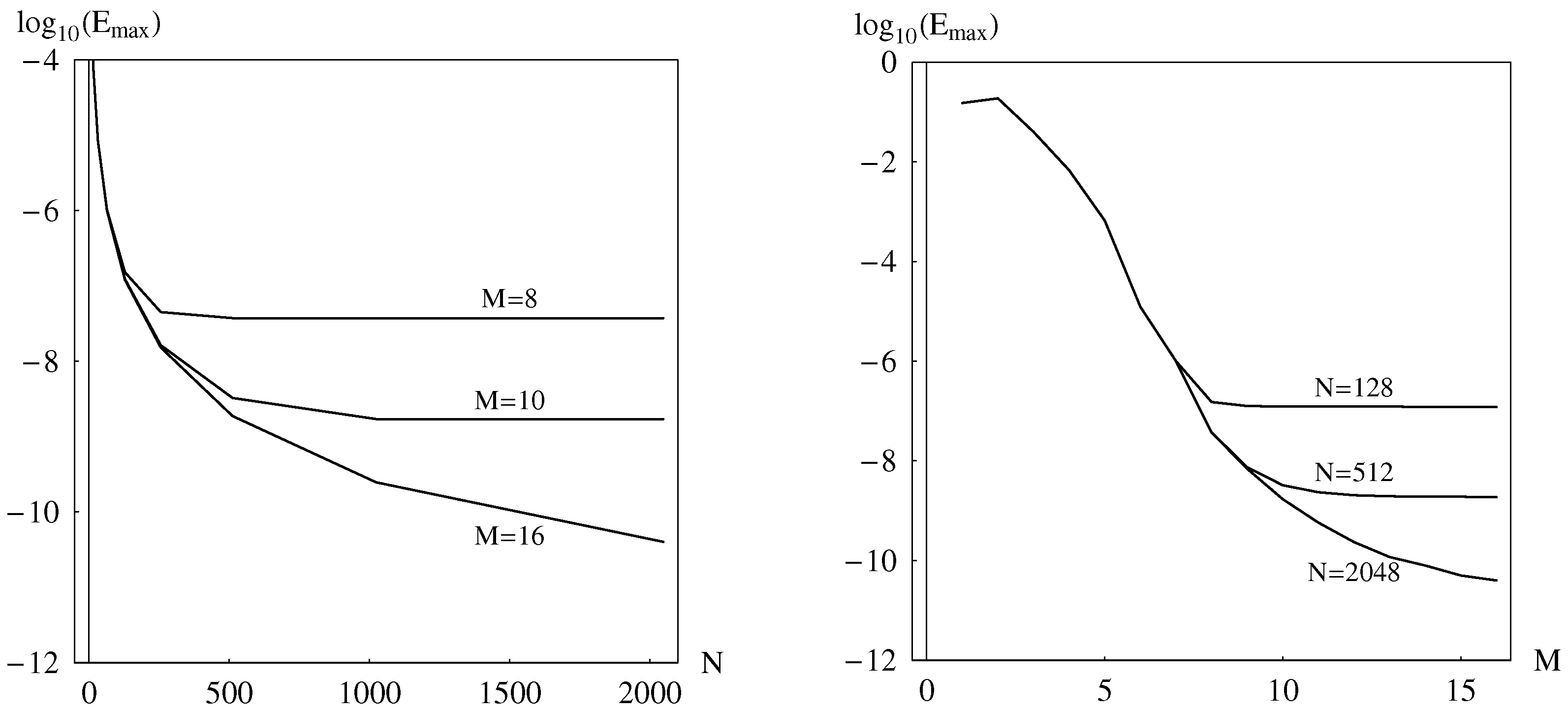
When M is small enough, it defines the accuracy of the approximate solution for all values of N. For N = 32 , the accuracy remains the same for the growth of M > 8 . On the other hand, when N = 512 , the calculated error decreases with the increase of M in the whole range 2 M 12 . This means that 512 Fourier’s harmonics provide an accurate approximation and the main error here is caused by the solving of FODEs. From the last row of this table, it can be seen evidently that the proposed method has high rates of convergence for the MAE, which provides reasonably accurate approximations for the unknown variables. It should be noted here that, with the increasing of M and N, the CO becomes flat, which means that the errors do not change for very large M or N. The proposed algorithm converges to the stable results.
In Figure 1, the observed behavior of the error is shown in more detail. Let us consider the left-hand side of Figure 1. The graphics l o g ( E m a x ( N ) ) have the same origin for all fixed M. With the growth of N, the curves l o g ( E m a x ( N ) ) change shape depending on the fixed value of M.

6.1.3. Example 3

The third example solved here is the high order TFPDE
D t α u x , t + sin t 1 + t D t α 1 u x , t + cos t 1 + t D t α 2 u x , t + log 1 + t u x , t = sinh t 1 + t D t α 3 2 u x 2 x , t + cosh t 1 + t D t α 4 2 u x 2 x , t + 1 + t 2 2 u x 2 x , t + f x , t ,
where α = 21 , α 1 = π , α 2 = 5 , α 3 = 3 , α 4 = 2 . As far as 4 < α = 21 < 5 , the TFPDE needs the following five ICs:
i u t i x , t = 0 = u i x , i = 0 , 1 , 2 , 3 , 4 .
The equation is subjected to the BC
u x x = 0 , t π 2 u ( x = 0 , t ) = g W t , u x x = 1 , t + e 2 u ( x = 1 , t ) = g E t ,
where the functions f x , t , u i x , g W t , g E t can be easily computed from the following exact solution
u x , t = cos t cos x + cosh x .
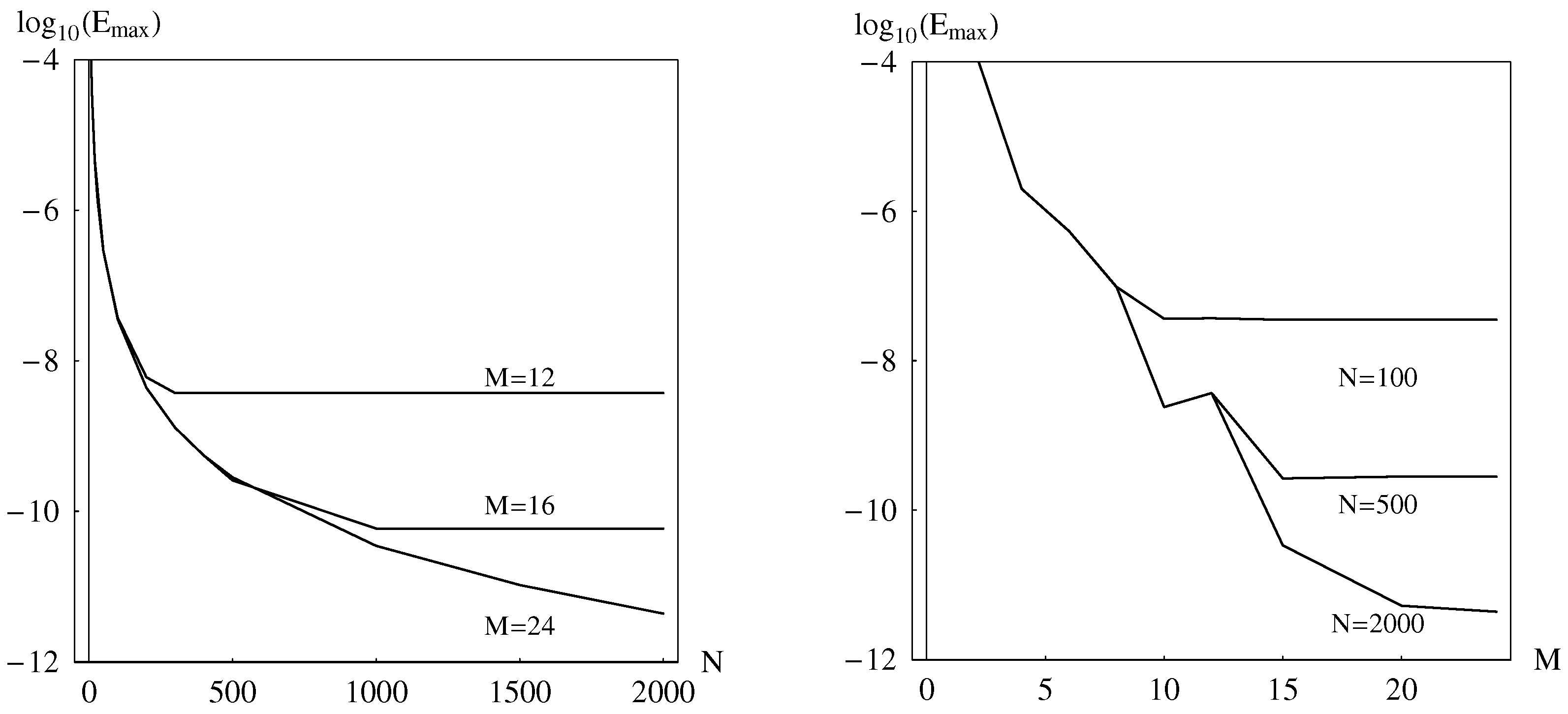
Table 4 presents the maximum absolute errors of the solution and its first derivative in time with the increase in N for M = 16 and M = 24 . In the case when M = 24 , the errors decrease sharply for 100 N 2000 . For M = 16 , the errors are the same for N > 500 . In Figure 2, this behavior of the error is shown in more detail.

6.2. ( 2 + 1 ) -Dimensional Problems

6.2.1. Example 4

Let us consider the following two-dimensional multi-term time-fractional mixed sub-diffusion and diffusion-wave equation defined in the unit square
D t α u x , y , t + u t x , y , t + D t α 1 u x , y , t + u x , y , t = 2 u x , y , t + D t α 2 2 u x , y , t + f x , y , t , x , y 0 , 1 2 ,
with the exact solution
u x , y , t = 1 + t 3 sin π x sin π y w t ψ 1 , 1 x , y ,
for the case α = 1.6 , α 1 = 0.7 , and α 2 = 0.3 .
The initial and Dirichlet boundary conditions of function f x , y , t conform the exact solution. Thus, we get the TFPDE with a single spatial harmonic corresponding to the eigenfunction ψ 1 , 1 x , y = 2 sin π x sin π y . As it is shown above, the problem can be reduced to the single FODE
D t α w t + d w t d t + D t α 1 w t + w t = 2 π 2 w t 2 π 2 D t α 2 w t + F t ,
with initial conditions w 0 = w 0 , d w 0 / d t = w 1 .
Table 5 shows the behavior of the MAE versus the M in φ m t = t δ m , δ m = σ m 1 . As shown in the previous section (see Equations (97), (98) and (107)), the approximate solution w t , M belongs to the linear span S α , σ , M = S p a n 1 , t , t α + σ m 1 m = 1 M . It is easy to check that for α = 1.6 , σ = 0.25 , there is no such M that the exact w t (see Equation (167)) belongs to S α , σ , M . On the other hand, w t S 1.6 , 0.35 , M 5 and w t S 1.6 , 0.7 , M 3 . The data placed in Table 5 illustrate this situation. For σ = 0.25 , the error decreases step-by-step with the growth of M, while it decreases sharply for σ = 0.35 and σ = 0.7 when the exact solution belongs to the corresponding manifold S α , σ , M . Feng, Liu, and Turner have considered this problem [32] and constructed two finite element schemes for its numerical solution. Ezz-Eldien et al. [55] have studied this problem by the use of the combination of the shifted Legendre polynomials with the time-space spectral collocation method. The comparison of the two methods presented in Table 4 of [55] shows that most accurate result that has been achieved there has the error E max = 1.407 × 10 3 for the first technique and E max = 1.807 × 10 6 for the second one.

6.2.2. Example 5

In this example, the problem solved here is to show the applicability of the proposed algorithm for the multi-term time-fractional diffusion-wave equation in the unit square 0 , 1 2 [56]
D t α u + u t + D t α 1 u + u = 2 u + f x , y , t .
The initial conditions, the Dirichlet BC, and the source term f correspond to the exact solution
u x , y , t = t 2 sin 1 x e x 1 sin 1 y e y 1 .
The data shown in Table 6 are obtained using α = 1.3 , α 1 = 0.3 , σ = 0.25 , and the numbers of the Müntz polynomials are M = 5 and M = 10 . The same problem was considered by Shen, Liu, and Anh in [56] using an implicit difference method. From this table, it is clearly stated that our new approach is generally more accurate than others, even with a small number of N and M.

6.3. ( 3 + 1 ) -Dimensional Problems

Example 6

Let us consider the following time-fractional telegraph equation in three dimensions
D t α + 1 u + D t α u + u = 2 u + f x , y , z , t , 0 t 1 ,
in the domain x , y , z 0 , π 3 with zero Dirichlet boundary conditions and the source term corresponding to the exact solution
u x , y , z , t = t α + 2 Γ α + 3 sin 2 x sin 2 y sin 2 z .
Using the transform x , y , z π x , π y , π z , the equation is transformed into
D t α + 1 u + D t α u + u = 1 π 2 2 u + f x , y , z , t ,
with the solution
u x , y , z , t = t α + 2 Γ α + 3 sin 2 π x sin 2 π y sin 2 π z .
Thus, we get a single spatial harmonic TFPDE. Substituting
u x , y , z , t = w t sin 2 π x sin 2 π y sin 2 π z ,
we get the FODE
D t α + 1 w + D t α w + 13 w = F t , 0 t 1 ,
with the source term and ICs corresponding to the exact solution
w t = t α + 2 Γ α + 3 .
Table 7 shows the behavior of the absolute errors with the growth of M for two cases: σ = 0.23 and σ = 0.25 . The results tabulated in the table are obtained by using α = 0.9 . As shown above (see Equations (97), (98) and (107)), the approximate solution w t , M belongs to the linear span S α , σ , M = S p a n 1 , t , t α + σ m 1 m = 1 M . It is easy to check that for σ = 0.23 there is no such M that the exact solution w t belongs to S α , σ , M . On the other hand, w t S α , 0.25 , M 5 . Indeed, α + 0.25 × 5 1 = α + 2 . The data placed in the table illustrate this situation. For σ = 0.23 , the error decreases step-by-step with the growth of M, while it decreases sharply for σ = 0.25 when the exact solution belongs to the corresponding manifold S α , σ , M . Yang et al. have considered this problem in [57] using an ADI finite difference scheme. The most accurate result shown in Table 2 of the reference has the error 1.1243 × 10 3 .

7. Conclusions

In the present work, an accurate method that can reach the computer rounding errors has been proposed for solving multi-term time-fractional equations. Let us note that the proposed analytical–numerical method collides with two key issues. The first one is the method to handle non-homogeneous time-dependent boundary conditions, which is critical to the derivation of v g . The second problem is the method to handle the non-homogeneous time-dependent source term of the equation. The derived function v g solves the first problem cardinally. This article presents the analytical function v g exactly satisfying the boundary conditions. Let us note that this function is not unique because one can locally change it inside the cube. The algorithm can give the function in the explicit analytical form with the help of math software packages like Maple or Mathematica if needed. The method of the Laplace transform and the Green function method are traditionally used for solving the second one. The BSM technique can also handle the non-homogeneous time-dependent source term. As mentioned above, in the solution procedure of the present method, one gets the system of the equation for each Fourier harmonic. The FODEs were solved independently with the help of Müntz polynomial bases. Additionally, the Fourier expansion of the source term over the eigenfunction basis should be performed at several fixed time moments t j only. The number of these points is proportional to M. The value of M is not too large. As the numerical experiment shows, even M = 10 for Müntz’s basis functions are enough for a rather precise approximate solution of the ( 3 + 1 ) multi-term FPDE of the high order. And the convergence order with respect to the M and N is larger than 3. Generally speaking, M > 10 and N > 100 are sufficient to provide accurate results for the tested problems.
In this paper, the method is demonstrated by solving an important class of fractional problems described in the Introduction. This technique can also be extended onto iterative quasi-linear PDEs and onto the problems in other orthogonal coordinate systems. The main drawback of this work is that the derivation of v g is only applicable for regular domains. Actually, numerical methods can be used for this purpose. This is the subject of further study.

Author Contributions

Conceptualization, J.L. (Ji Lin), S.R. and J.L. (Jun Lu); methodology, Y.Z.; writing—original draft preparation, S.R.; writing—review and editing, J.L. (Ji Lin) and Y.S.; visualization, J.L. (Ji Lin); funding acquisition, J.L. (Jun Lu). All authors have read and agreed to the published version of the manuscript.

Funding

This research was funded by the National Key Research and Development Program of China (No. 2021YFB2600704), the National Natural Science Foundation of China (Nos. 12072103, 52171272), and the Significant Science and Technology Project of the Ministry of Water Resources of China (No. SKS-2022112).

Data Availability Statement

No data were analyzed or generated during the study.

Conflicts of Interest

The authors declare no conflict of interest.

References

  1. Hilfer, R. Applications of Fractional Calculus in Physics; World Scientific: Singapore, 2000. [Google Scholar]
  2. Molz, F.-J.; Liu, H.-H.; Szulga, J. Fractional Brownian motion and fractional Gaussian noise in subsurface hydrology: A review, presentation of fundamental properties, and extensions. Water Resour. Res. 1997, 33, 2273–2286. [Google Scholar] [CrossRef]
  3. Singh, J.; Kumar, D.; Baleanu, D. On the analysis of chemical kinetics system pertaining to a fractional derivative with Mittag-Leffler type kernel. Chaos Interdiscip. J. Nonlinear Sci. 2017, 27, 103113. [Google Scholar] [CrossRef]
  4. Podlubny, I. Fractional Differential Equations; Academic Press: Cambridge, MA, USA, 1999. [Google Scholar]
  5. Langlands, T.-A.-M.; Henry, B.I.; Wearne, S.L. Fractional cable equation models for anomalous electrodiffusion in nerve cells: Finite domain solutions. Siam J. Appl. Math. 2011, 71, 1168–1203. [Google Scholar] [CrossRef]
  6. Chen, Y.; Chen, C.-M. Novel numerical method of the fractional cable equation. J. Appl. Math. Comput. 2020, 62, 663–683. [Google Scholar] [CrossRef]
  7. Dehghan, M.; Shafieeabyaneh, N.; Abbaszadeh, M. Application of spectral element method for solving Sobolev equations with error estimation. Appl. Numer. Math. 2020, 158, 439–462. [Google Scholar] [CrossRef]
  8. Zhao, J.; Fang, Z.; Li, H.; Liu, Y. A Crank–Nicolson Finite Volume Element Method for Time Fractional Sobolev Equations on Triangular Grids. Mathematics 2020, 8, 1591. [Google Scholar] [CrossRef]
  9. Lin, J.; Zhang, Y.-H.; Reutskiy, S. A semi-analytical method for 1D, 2D and 3D time fractional second order dual-phase-lag model of the heat transfer. Alex. Eng. J. 2021, 60, 5879–5896. [Google Scholar] [CrossRef]
  10. Sun, H.-G.; Zhang, Y.; Baleanu, D.; Chen, W.; Chen, Y.-Q. A new collection of real world applications of fractional calculus in science and engineering. Commun. Nonlinear Sci. Numer. Simul. 2018, 64, 213–231. [Google Scholar] [CrossRef]
  11. Liu, Y.; Zheng, L.; Zhang, X. Unsteady MHD Couette flow of a generalized Oldroyd-B fluid with fractional derivative. Comput. Math. Appl. 2011, 61, 443–450. [Google Scholar] [CrossRef]
  12. Ming, C.; Liu, F.-W.; Zheng, L.; Turner, I.; Anh, V. Analytical solutions of multi-term time fractional differential equations and application to unsteady flows of generalized viscoelastic fluid. Comput. Math. Appl. 2016, 72, 2084–2097. [Google Scholar] [CrossRef]
  13. Ding, X.-L.; Nieto, J.-J. Analytical solutions for multi-term time-space fractional partial differential equations with nonlocal damping terms. Fract. Calc. Appl. Anal. 2018, 21, 312–335. [Google Scholar]
  14. Ding, X.-L.; Jiang, Y.-J. Analytical solutions for multi-term time-space coupling fractional delay partial differential equations with mixed boundary conditions. Commun. Nonlinear Sci. Numer. Simul. 2018, 65, 231–247. [Google Scholar] [CrossRef]
  15. Jong, S.-G.; Choe, H.-C.; Ri, Y.-D. A new approach for an analytical solution for a system of multi-term linear fractional differential equations. Iran. J. Sci. Technol. Trans. Sci. 2021, 45, 955–964. [Google Scholar] [CrossRef]
  16. Jiang, H.; Liu, F.; Turner, I.; Burrage, K. Analytical solutions for the multi-term time-fractional diffusion-wave/diffusion equations in a finite domain. Comput. Math. Appl. 2012, 64, 3377–3388. [Google Scholar] [CrossRef]
  17. Zeli, V.; Zorica, D. Analytical and numerical treatment of the heat conduction equation obtained via time-fractional distributed-order heat conduction law. Phys. Stat. Appl. 2018, 492, 2316–2335. [Google Scholar] [CrossRef]
  18. Ama, E.-S.; El-Kalla, I.-L.; Ziada, E. Analytical and numerical solutions of multi-term nonlinear fractional orders differential equations. J. Appl. Math. Comput. 2010, 60, 788–797. [Google Scholar]
  19. Liu, D.; He, W. Numerical simulation analysis mathematics of fluid mechanics for semiconductor circuit breaker. Appl. Math. Nonlinear Sci. 2021, 7, 331–342. [Google Scholar] [CrossRef]
  20. Yang, Y. Application of numerical method of functional differential equations in fair value of financial accounting. Appl. Math. Nonlinear Sci. 2022, 7, 533–540. [Google Scholar] [CrossRef]
  21. Liu, Q.; Dai, B.; Katib, I.; Alhamami, M.-A. Financial accounting measurement model based on numerical analysis of rigid normal differential equation and rigid generalised functional equation. Appl. Math. Nonlinear Sci. 2022, 7, 541–548. [Google Scholar] [CrossRef]
  22. Xu, L.; Aouad, M. Application of Lane-Emden differential equation numerical method in fair value analysis of financial accounting. Appl. Math. Nonlinear Sci. 2021, 7, 669–676. [Google Scholar] [CrossRef]
  23. Yan, L.; Sabir, Z.; Ilhan, E.; Gao, W. Design of a computational heuristic to solve the nonlinear Liénard differential model: Nonlinear Liénard differential model. CMES-Comput. Model. Eng. Sci. 2023, 136, 201–221. [Google Scholar]
  24. Fardi, M.; Zaky, M.-A.; Hendy, A.-S. Nonuniform difference schemes for multi-term and distributed-order fractional parabolic equations with fractional Laplacian. Math. Comput. Simul. 2023, 206, 614–635. [Google Scholar] [CrossRef]
  25. Mohammadi, S.; Ghasemi, M.; Fardi, M. A fast Fourier spectral exponential time-differencing method for solving the time-fractional mobile–immobile advection–dispersion equation. Comput. Appl. Math. 2022, 41, 264. [Google Scholar] [CrossRef]
  26. Fardi, M.; Khan, Y. A fast difference scheme on a graded mesh for time-fractional and space distributed-order diffusion equation with nonsmooth data. Int. J. Mod. Phys. B 2022, 36, 2250076. [Google Scholar] [CrossRef]
  27. Fardi, M.; Alidousti, J. A Legendre spectral-finite difference method for Caputo–Fabrizio time-fractional distributed-order diffusion equation. Math. Sci. 2022, 16, 417–430. [Google Scholar] [CrossRef]
  28. Fardi, M.; Ghasemi, M. A numerical solution strategy based on error analysis for time-fractional mobile/immobile transport model. Soft Comput. 2021, 25, 11307–11331. [Google Scholar] [CrossRef]
  29. Fardi, M.; Khan, Y. A novel finite difference-spectral method for fractal mobile/immobiletransport model based on Caputo–Fabrizio derivative. Chaos Solitons Fractals 2021, 143, 110573. [Google Scholar] [CrossRef]
  30. Dehghan, M.; Safarpoor, M.; Abbaszadeh, M. Two high-order numerical algorithms for solving the multi-term time fractional diffusion-wave equations. J. Comput. Appl. Math. 2015, 290, 174–195. [Google Scholar] [CrossRef]
  31. Jin, B.; Lazarov, R.; Liu, Y.; Zhou, Z. The Galerkin finite element method for a multi-term time-fractional diffusion equations. J. Comput. Phys. 2015, 281, 825–843. [Google Scholar] [CrossRef]
  32. Feng, L.-B.; Liu, F.-W.; Turner, I. Finite difference/finite element method for a novel 2D multi-term time-fractional mixed sub-diffusion and diffusion-wave equation on convex domains. Commun. Nonlinear Sci. Numer. Simul. 2019, 70, 354–371. [Google Scholar] [CrossRef]
  33. Yin, B.-L.; Liu, Y.; Li, H.; Zeng, F.-H. A class of efficient time-stepping methods for multi-term time-fractional reaction-diffusion-wave equations. Appl. Numer. Math. 2021, 165, 56–82. [Google Scholar] [CrossRef]
  34. Zeng, F.; Zhang, Z.; Karniadakis, G.E. Second-order numerical methods for multi-term fractional differential equations: Smooth and non-smooth solutions. Comput. Methods Appl. Mech. Eng. 2017, 327, 478–502. [Google Scholar] [CrossRef]
  35. Zheng, M.; Liu, F.; Anh, V.; Turner, I. A high-order spectral method for the multi-term time-fractional diffusion equations. Appl. Math. Model. 2016, 40, 4970–4985. [Google Scholar] [CrossRef]
  36. Rashidinia, J.; Mohmedi, E. Approximate solution of the multi-term time fractional diffusion and diffusion-wave equations. Comput. Math. Appl. 2020, 39, 216. [Google Scholar] [CrossRef]
  37. Soltani, J.-A.; Derakhshan, M.-H.; Marasi, H.-R. An efficient hybrid numerical method for multi-term time fractional partial differential equations in fluid mechanics with convergence and error analysis. Commun. Nonlinear Sci. Numer. 2022, 114, 106620. [Google Scholar]
  38. Alsuyuti, M.-M.; Doha, E.-H.; Ezz-Eldien, S.-S. Galerkin operational approach for multi-dimensions fractional differential equations. Commun. Nonlinear Sci. Numer. 2022, 114, 106608. [Google Scholar] [CrossRef]
  39. Fardi, M. A kernel-based pseudo-spectral method for multi-term and distributed order time-fractional diffusion equations. Numer. Methods Partial. Differ. Equations 2022. [Google Scholar] [CrossRef]
  40. Fardi, M.; Al-Omari, S.-K.-Q.; Araci, S. A pseudo-spectral method based on reproducing kernel for solving the time-fractional diffusion-wave equation. Adv. Contin. Discret. Model. 2022, 2022, 54. [Google Scholar] [CrossRef]
  41. Carslaw, H.-S.; Jaeger, J.-C. Conduction of Heat in Solids; Clarendon Press: Oxford, UK, 1959. [Google Scholar]
  42. Alquran, M.; Ali, M.; Alsukhour, M.; Jaradat, I. Promoted residual power series technique with Laplace transform to solve some time-fractional problems arising in physics. Results Phys. 2020, 19, 103667. [Google Scholar] [CrossRef]
  43. Kamran, K.; Shah, Z.; Kumam, P.; Alreshidi, N.-A. A Meshless Method Based on the Laplace Transform for the 2D Multi-Term Time Fractional Partial Integro-Differential Equation. Mathematics 2020, 8, 1972. [Google Scholar] [CrossRef]
  44. Reutskiy, S.-Y.; Fu, Z.-J. A semi-analytic method for fractional-order ordinary differential equations: Testing results. Fract. Calc. Appl. Anal. 2018, 21, 1598–1618. [Google Scholar] [CrossRef]
  45. Hong, Y.-X.; Lin, J.; Chen, W. A typical backward substitution method for the simulation of Helmholtz problems in arbitrary 2D domains. Eng. Anal. Bound. Elem. 2018, 93, 167–176. [Google Scholar] [CrossRef]
  46. Safari, F.; Azarsa, P. Backward substitution method based on Müntz polynomials for solving the nonlinear space fractional partial differential equations. Math. Methods Appl. Sci. 2020, 43, 847–864. [Google Scholar] [CrossRef]
  47. Zhang, Y.; Rabczuk, T.; Lu, J.; Lin, S.; Lin, J. Space-time backward substitution method for nonlinear transient heat conduction problems in functionally graded materials. Comput. Math. Appl. 2022, 124, 98–110. [Google Scholar] [CrossRef]
  48. Lin, J.; Xu, Y.; Zhang, Y. Simulation of linear and nonlinear advection–diffusion–reaction problems by a novel localized scheme. Appl. Math. Lett. 2020, 99, 106005. [Google Scholar] [CrossRef]
  49. Lin, J.; Xu, Y.; Reutskiy, S.; Lu, J. A novel Fourier-based meshless method for (3 + 1)-dimensional fractional partial differential equation with general time-dependent boundary conditions. Appl. Math. Lett. 2023, 135, 108441. [Google Scholar] [CrossRef]
  50. Esmaeili, S.; Shamsi, M.; Luchko, Y. Numerical solution of fractional differential equations with a collocation method based on Müntz polynomials. Comput. Math. Appl. 2011, 62, 918–929. [Google Scholar] [CrossRef]
  51. Mokhtary, P.; Ghoreishi, F.; Srivastava, H.M. The Müntz-Legendre Tau method for fractional differential equations. Appl. Math. Model. 2016, 40, 671–684. [Google Scholar] [CrossRef]
  52. Bahmanpour, M.; Tavassoli-Kajani, M.; Maleki, M. A Müntz wavelets collocation method for solving fractional differential equations. Comput. Math. Appl. 2018, 37, 5514–5526. [Google Scholar] [CrossRef]
  53. Maleknejad, K.; Rashidinia, J.; Eftekhari, T. Numerical solutions of distributed order fractional differential equations in the time domain using the Müntz–Legendre wavelets approach. Numer. Methods Partial. Differ. Equations 2021, 37, 707–731. [Google Scholar] [CrossRef]
  54. Yang, X.; Jiang, X.Y.; Zhang, H. A time–space spectral tau method for the time fractional cable equation and its inverse problem. Appl. Numer. Math. 2018, 130, 95–111. [Google Scholar] [CrossRef]
  55. Ezz-Eldien, S.-S.; Doha, E.-H.; Wang, Y.; Cai, W. A numerical treatment of the two-dimensional multi-term time-fractional mixed sub-diffusion and diffusion-wave equation. Commun. Nonlinear Sci. Numer. Simul. 2020, 91, 105445. [Google Scholar] [CrossRef]
  56. Shen, S.; Liu, F.-W.; Anh, V.-V. The analytical solution and numerical solutions for a two-dimensional multi-term time fractional diffusion and diffusion-wave equation. J. Comput. Appl. Math. 2019, 345, 515–534. [Google Scholar] [CrossRef]
  57. Yang, X.-H.; Qiu, W.-L.; Zhang, H.-X.; Tang, L. An efficient alternating direction implicit finite difference scheme for the three-dimensional time-fractional telegraph equation. Comput. Math. Appl. 2021, 102, 233–247. [Google Scholar] [CrossRef]
Figure 1. The MAE with respect to the parameters M and N.
Mathematics 11 00929 g001
Figure 2. The MAE with respect to the parameters M and N.
Mathematics 11 00929 g002
Table 1. The MAE versus the M at t = 1 for different σ .
M12345610
σ = 0.251.19 × 10 2 1.93 × 10 3 1.97 × 10 4 3.73 × 10 5 1.22 × 10 16 1.22 × 10 16 -
σ = 0.501.19 × 10 2 1.47 × 10 3 1.22 × 10 16 1.22 × 10 16 ---
σ = 0.331.19 × 10 2 1.83 × 10 3 1.21 × 10 4 9.35 × 10 7 5.44 × 10 8 6.38 × 10 9 3.12 × 10 1
Table 2. The MAE, C O N , and the elapsed time versus the N using M = 7 (left) and M = 15 (right).
M = 7 M = 15
N E m a x C O N C P U , s E m a x C O N C P U , s
29.37 × 10 2 -0.029.37 × 10 2 -0.11
47.31 × 10 3 3.680.077.31 × 10 3 3.680.17
86.81 × 10 4 3.420.166.81 × 10 4 3.420.33
167.30 × 10 5 3.220.367.22× 10 5 3.240.66
329.09 × 10 6 3.010.618.30 × 10 6 3.121.0
641.78 × 10 6 2.350.989.94 × 10 7 3.061.9
1289.97 × 10 7 0.841.841.22 × 10 7 3.034.1
2569.94 × 10 7 0.043.181.51 × 10 8 3.019.0
5129.94 × 10 7 <<16.51.89 × 10 9 2.9919
10249.94 × 10 7 <<1132.57 × 10 10 2.8844
20489.94 × 10 7 <<1245.36 × 10 11 2.2674
[54], Table 2, E max = 3.2279 × 10 5
Table 3. The MAE and C O M versus the M with the fixed number of harmonics N.
N = 32 N = 128 N = 512
M E m a x C O M E m a x C O M E m a x C O M
21.87 × 10 1 -1.87 × 10 1 -1.87 × 10 1 -
34.02 × 10 2 3.794.02 × 10 2 3.794.02 × 10 2 3.79
46.69 × 10 3 6.236.69 × 10 3 6.236.69 × 10 3 6.23
56.66 × 10 4 10.36.66 × 10 4 10.36.66 × 10 4 10.3
61.82 × 10 5 19.71.24 × 10 5 21.81.24 × 10 5 21.8
79.09 × 10 6 4.59.97 × 10 7 16.49.97 × 10 7 16.4
88.33 × 10 6 0.661.51 × 10 7 14.13.72 × 10 8 24.6
98.30 × 10 6 <<11.27 × 10 7 1.477.42 ×10 9 13.7
108.30 × 10 6 <<11.23 × 10 7 0.083.22 × 10 9 7.92
118.30 × 10 6 <<11.22 × 10 7 <<12.33 × 10 9 3.39
128.30 × 10 6 <<11.22 × 10 7 <<11.96 × 10 9 0.63
Table 4. The MAE of the u and u / t versus N using M = 16 (left) and 24 (right).
M = 16 M = 24
N E m a x u E m a x u / t E H 1 E m a x u E m a x u / t E H 1
1003.53 × 10 8 5.51 × 10 8 8.43 × 10 9 3.53 × 10 8 5.51 × 10 8 8.42 × 10 9
2004.36 × 10 9 6.92 × 10 9 8.16 × 10 10 4.39 × 10 9 6.84 × 10 9 7.33 × 10 10
3001.27 × 10 9 2.10 × 10 9 3.93 × 10 10 1.30 × 10 9 2.02 × 10 9 1.76 × 10 10
4005.21 × 10 10 9.31 × 10 10 3.56 × 10 10 5.47 × 10 10 8.51 × 10 10 6.42 × 10 11
5002.54 × 10 10 5.15 × 10 10 3.51 × 10 10 2.80 × 10 10 4.36 × 10 10 2.94 × 10 11
10005.80 × 10 11 1.94 × 10 10 3.50 × 10 10 3.49 × 10 11 5.44 × 10 11 2.59 × 10 12
20005.80 × 10 11 1.94 × 10 10 3.50 × 10 10 4.35 × 10 12 6.81 × 10 12 2.65 × 10 13
Table 5. The MAE and the computational time versus the M at t = 1 .
M1234561015
σ = 0.254.3 × 10 1 4.8 × 10 2 1.1 × 10 2 1.7 × 10 3 8.5 × 10 5 2.2 × 10 6 8.1 × 10 11 5.4 × 10 13
σ = 0.354.3 × 10 1 3.6 × 10 2 5.2 × 10 3 4.9 × 10 4 1.8 × 10 15 1.1 × 10 15 --
σ = 0.704.3 × 10 1 1.8 × 10 2 1.1 × 10 15 2.0 × 10 15 ----
Table 6. The MAE and the elapsed time versus the N at t = 1 using M = 5 (left) and 10 (right).
M = 5 M = 10
N E m a x u E m a x u / t CPU, s E m a x u E m a x u / t CPU, s
1001.443 × 10 6 3.105 × 10 6 91.452 × 10 6 2.903 × 10 6 14
2002.018 × 10 7 1.553 × 10 6 232.100 × 10 7 4.200 × 10 7 35
3001.203 × 10 7 1.522 × 10 6 566.445 × 10 8 1.289 × 10 7 97
4001.231 × 10 7 1.514 × 10 6 892.756 × 10 8 5.510 × 10 8 154
5001.241 × 10 7 1.511 × 10 6 1531.420 × 10 8 2.839 × 10 8 260
6001.245 × 10 7 1.510 × 10 6 2048.247 × 10 9 1.649 × 10 8 352
[56], Table 1, E max u = 6.145893072032060 × 10 6
Table 7. The MAE versus M at t = 1 for different σ .
M1234561015
σ = 0.234.6 × 10 2 2.4 × 10 2 3.4 × 10 3 1.2 × 10 4 1.6 × 10 6 1.2 × 10 7 2.4 × 10 10 3.9 × 10 12
σ = 0.254.6 × 10 2 2.3 × 10 2 3.0 × 10 3 8.2 × 10 5 1.1 × 10 17 2.8 × 10 17 --
Disclaimer/Publisher’s Note: The statements, opinions and data contained in all publications are solely those of the individual author(s) and contributor(s) and not of MDPI and/or the editor(s). MDPI and/or the editor(s) disclaim responsibility for any injury to people or property resulting from any ideas, methods, instructions or products referred to in the content.

