Article

Compression Reconstruction Network with Coordinated Self-Attention and Adaptive Gaussian Filtering Module

1
School of Information Engineering, Nanchang University, Nanchang 330031, China
2
Qiyuan Lab, Beijing 100095, China
*
Author to whom correspondence should be addressed.
Mathematics 2023, 11(4), 847; https://doi.org/10.3390/math11040847
Submission received: 30 December 2022 / Revised: 27 January 2023 / Accepted: 3 February 2023 / Published: 7 February 2023
(This article belongs to the Special Issue Advances in Computer Vision and Machine Learning)

Abstract

:
Although compressed sensing theory has many advantages in image reconstruction, its reconstruction and sampling time is very long. Fast reconstruction of high-quality images at low measurement rates is the direction of the effort. Compressed sensing based on deep learning provides an effective solution for this. In this study, we propose an attention-based compression reconstruction mechanism (ACRM). The coordinated self-attention module (CSAM) is designed to be embedded in the main network consisting of convolutional blocks and utilizes the global space and channels to focus on key information and ignore irrelevant information. An adaptive Gaussian filter is proposed to solve the loss of multi-frequency components caused by global average pooling in the CSAM, effectively supplementing the network with different frequency information at different measurement rates. Finally, inspired by the basic idea of the attention mechanism, an improved loss function with attention mechanism (AMLoss) is proposed. Extensive experiments show that the ACRM outperforms most compression reconstruction algorithms at low measurement rates.

1. Introduction

In 2004, E.J. Candes, J. Romberg, T. Tao, and D.L. Donoho proposed the compressed sensing theory. The theory shows that if a signal is sparse or compressible in a certain transform domain, it can be recovered accurately from measurements less than those of the Nyquist sampling theorem [1,2,3,4,5]. The compressed sensing theory defines a new paradigm for signal acquisition and reconstruction [6]. Our work focuses on compressed sensing techniques for fast reconstruction of high-quality images at low measurement rates, such as single pixel imaging techniques [7,8,9] and MRI [10,11].
Despite compressed sensing having many advantages, its sampling and reconstruction time is very long. Traditional compressive reconstruction algorithms such as convex relaxation methods [12], greedy matching pursuit methods [13], and iterative thresholding algorithms are too computationally complex, and the reconstruction time increases exponentially with the resolution of the image [14,15]. In recent years, researchers have begun to use deep learning methods to solve the reconstruction problem of compressed measurements. Deep learning can learn the structural features of the signal and adjust the network weights in a data-driven manner adaptively, enabling the reconstruction of raw images from low-dimensional measurement data without extensive computation [16]. Compared with the traditional iterative algorithm, the reconstruction method based on deep learning not only avoids the huge amount of computation effectively but also obtains better reconstruction quality. This provides a solution for image reconstruction based on compressed sensing. Therefore, compressed sensing technology based on deep learning has also attracted much attention and become a research hotspot.
Most of the existing deep learning networks for compressed sensing rely on massive data streams and deeper convolutional layers to obtain higher receptive fields and high-quality reconstructions. Many data calculations cause data redundancy, which reduces the reconstruction rate and efficiency greatly [17]. The reconstruction quality of the important regions of the image may be worse, thereby lowering the reconstruction quality.
In this study, an attention-based compression reconstruction mechanism (ACRM) is proposed, which enables the network to learn important information of images and suppress useless information autonomously. The reconstruction quality of the network is improved greatly. Extensive experiments show that the ACRM outperforms most compression reconstruction algorithms at a low measurement rate. Our proposed attention mechanism and adaptive Gaussian filtering also outperforms other mainstream attention modules in this field. Our contributions are as follows:
  • We propose a coordinated self-attention module (CSAM), which not only introduces information into the channel and the spatial domain but also captures the global information of the image, improving the network’s ability to capture long-range relationships for better imaging results.
  • We propose an adaptive Gaussian filter sub-network in the frequency domain to make up for the defect of global average pooling in the CSAM. It can capture information on different frequency components of the image selectively when the measurement rate is changed.
  • We propose a loss function with attention based on the traditional MSE-Loss (AMLoss) to match the gradient descent algorithm with the attention mechanism and focus more on the important parts of the image during optimization. Extensive experiments prove that the AMLoss can significantly improve the reconstruction quality.

2. Background and Related Work

This section mainly introduces the development of the compressed sensing imaging and the development of the attention mechanism.

2.1. Deep Learning Based on Compressed Sensing Reconstruction

The process of image reconstruction is the process of finding solutions to underdetermined equations. There are infinite solutions to this problem in theory. However, the reconstruction of image x can be carried out by solving the L 0 norm problem based on compressed sensing theory. Let x equal Ψ α , where Ψ is an orthonormal basis and the number of non-zero elements of α is much less than N ( N refers to the dimension of image x ). The image reconstruction problem can be expressed as
y = m i n α 0     s . t .     Φ Ψ α .
where Φ is the observation matrix, which projects the high-dimensional signal x into the low-dimensional space.
Traditional compressed sensing reconstruction methods are based on sparse prior knowledge to iteratively reconstruct the original signal by solving an optimization problem. They are mainly convex relaxation methods [12], greedy matching pursuit methods [13], and Bayesian methods [18], aiming at the problem that the sparse assumption model in traditional compressive sensing theory is not fully satisfied in practical applications. The deep learning method uses a data-driven approach to learn signal structure features, relaxes the assumptions on the sparseness of the original signal, and learns the specific structure of the actual signal by adaptively adjusting the network weights. At the same time, the measurement and reconstruction process can be turned into an end-to-end framework.
In 2015, Mousavi et al. used stacked denoising autoencoders as unsupervised feature learners to achieve fast reconstruction of compressed sensing images [19]. In 2016, Kulkarni et al. proposed the ReconNet model based on image super-resolution reconstruction, which improved the accuracy of reconstructed images [16]. In 2017, Mousavi et al. proposed the DeepInverse deep learning model [20]. In the same year, Yao et al. used the ResNet structure to build a deep residual reconstruction network named DR2-Net based on the ReconNet, which once again improved the accuracy of the reconstructed images [17]. In 2018, S. Lohit et al. proposed a variant of the ReconNet that used an adversarial loss to further improve the reconstruction quality [21]. In 2020, Yang et al. proposed the ADMM-SCNet, which used traditional model-based compressed sensing methods and data to drive deep learning methods for reconstructing images from sparsely sampled measurements. The method achieves good reconstruction accuracy at fast computation speed [22]. In the same year, inspired by generative networks and attention mechanisms, Yuan et al. proposed a down-sampled MRI reconstruction method based on SARA-GAN. The method applies the relative average discriminator theory to make full use of prior knowledge. At the same time, adding the self-attention mechanism in the upper layers of the generator can overcome the problem of limited convolution kernel size [23]. In 2021, Zhang et al. proposed a deep learning system for attention-guided dual-layer image compression (AGDL), which advanced the state of the art in perceptual image compression [24]. In the same year, Barranca formulated a new framework for learning improved sampling paradigms for compressed sensing in a bio motivated manner, significantly improving the quality of signal reconstruction across multiple connection weight penalty schemes and signal classes [25].

2.2. Attention

In recent years, attention mechanisms have been seen in various types of tasks, such as image processing, machine translation, and natural language processing. The attention mechanism, as its name implies, draws on the unique brain processing signal mechanism of human vision [26]. In computer vision, the attention mechanism can filter out important regions of the input image and extract important information from key parts [27]. It is a means of sifting out high-value information from a large volume of information, which is widely used in the field of remote sensing [28,29].
Convolutional neural networks (CNNs) have been shown to be effective models for a wide range of vision tasks. They can generate image representations that capture hierarchical patterns and obtain global theoretical receptive fields. If researchers want to find the correlation between two parts of an image that are far apart, then they generally continue to increase the number of convolutional layers and the number of pooling layers, which will increase the cost of computation and the number of parameters. Then, Wang et al. proposed the non-local network in the spatial domain based on the self-attention mechanism. Each pixel on the image has an attention map, which increases its ability to obtain global information [30]. Global information refers to the information containing the dependencies between image elements. However, this model requires a large amount of computation. Cao et al. found in the experiment that the attention map of each pixel in an image is the same, so a simple module GC-Net that shares the attention map was constructed. This module reduces the amount of computation greatly [31]. Many of the previous works have proposed structures in the spatial domain that can improve network performance, and the SE-Net is the first attention mechanism module proposed at the channel domain. It can complete the weight labeling of features in the channel dimension dynamically and adaptively, paying attention to the dependencies at the channel level of the model. Most importantly, the SE-Net is very simple in construction and easy to deploy without introducing new functions or layers [32]. However, the SE-Net module needs to reduce the amount of calculation by reducing the dimensionality of the fully connected layer, which will weaken the learning of weights. Therefore, Wang et al. proposed the ECA-Net based on the SE-Net, which uses a local cross-channel interaction strategy without dimensionality reduction. It can improve cross-channel interactive learning while avoiding dimensionality reduction, making the module lighter [33]. Today, global average pooling in the SE module has become a common spatial information-encoding method. However, it saves the global spatial information in a channel descriptor, which makes it difficult to save the position information. Hou et al. then proposed to decompose the global average pooling into one-dimensional average pooling in parallel along the horizontal and vertical directions. Perceptual feature maps along two independent directions are obtained, which in turn encode the feature maps into two attention maps. Then the position information is stored in the generated attention map [34]. This method can capture not only inter-channel information, but also orientation-aware and position-sensitive information.
Inspired by the coordinated attention module and the global context block that can improve long-distance capture capability [34,35], we designed the coordinated self-attention module (CSAM). While capturing inter-channel information and spatial location information, this module also enhances feature transformation and feature aggregation capabilities, which improves the reconstruction capabilities of the network ultimately.

3. The Proposed Method

The main innovations of our work are to introduce a new attention mechanism into the field of compressed sensing imaging and propose a new interpretable loss function. In this section, we will describe the proposed method in detail, including model formula and the proof of loss function principle.

3.1. Overall Network Framework

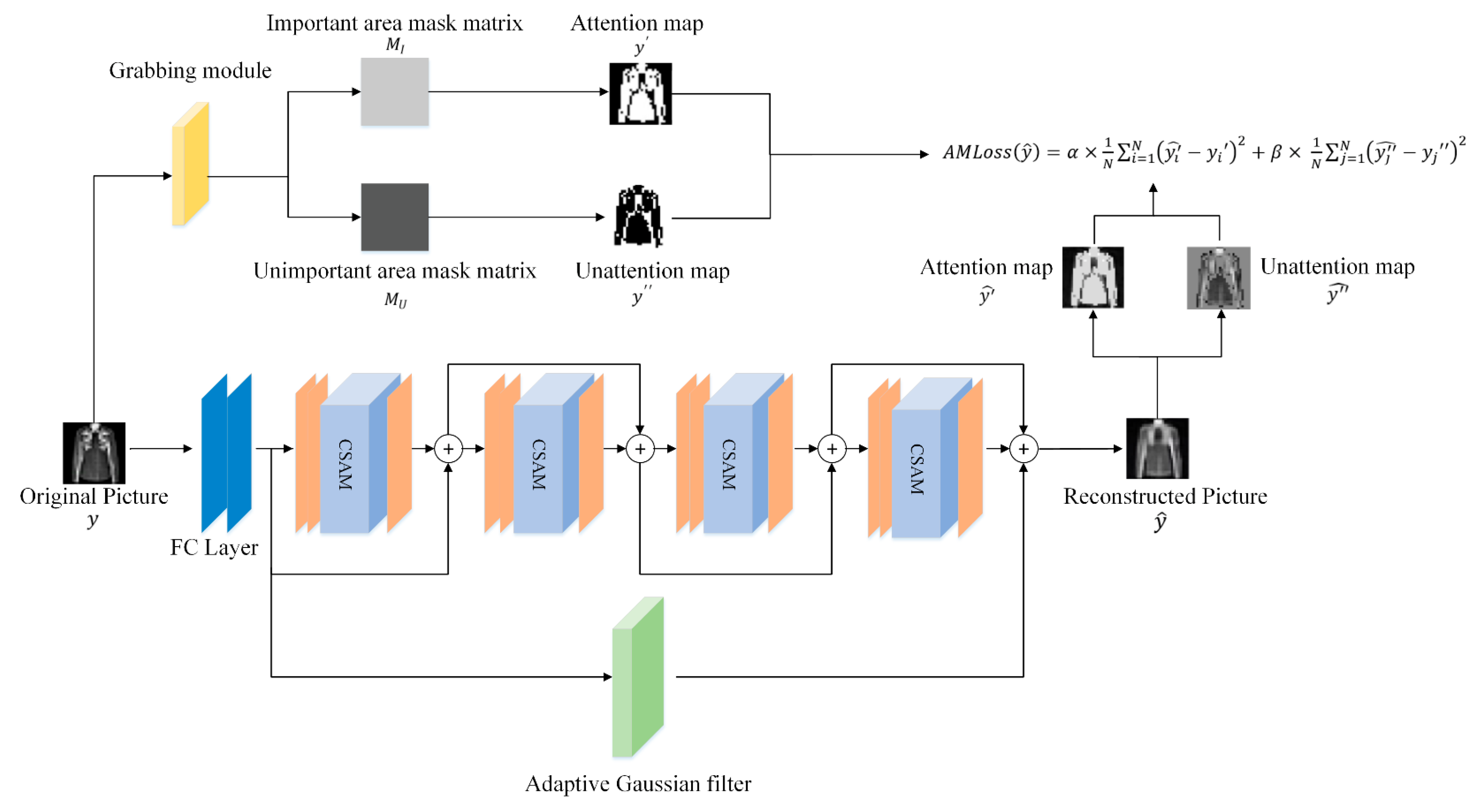
This part mainly introduces the structure of ACRM as shown in Figure 1. The network consists of two fully connected layers, four ACR submodules, and an adaptive Gaussian filter. The first fully connected layer is a sampling network used to down sample the original image to generate CS measurements [36]. The second fully connected layer is used for the preliminary reconstruction of the CS measurements [36]. Related studies have shown that using fully connected layers as linear mapping networks can reconstruct high-quality primary images [17] so that the subsequent deep convolution can proceed smoothly. The ACR submodule includes three convolutional layers and the CSAM. The convolution kernel sizes and channels of the three convolutional layers from left to right are 11 × 11 × 64, 7 × 7 × 32, and 3 × 3 × 1, respectively. After each convolutional layer, the LeakyReLU function is used to improve the ability of convolutional nonlinear feature extraction. Each ACR submodule uses a residual structure to cope with vanishing and exploding gradients. Next, we focus on the CSAM, the adaptive Gaussian filtering sub-network and the loss function used for network training.

3.2. Coordinated Self-Attention Module

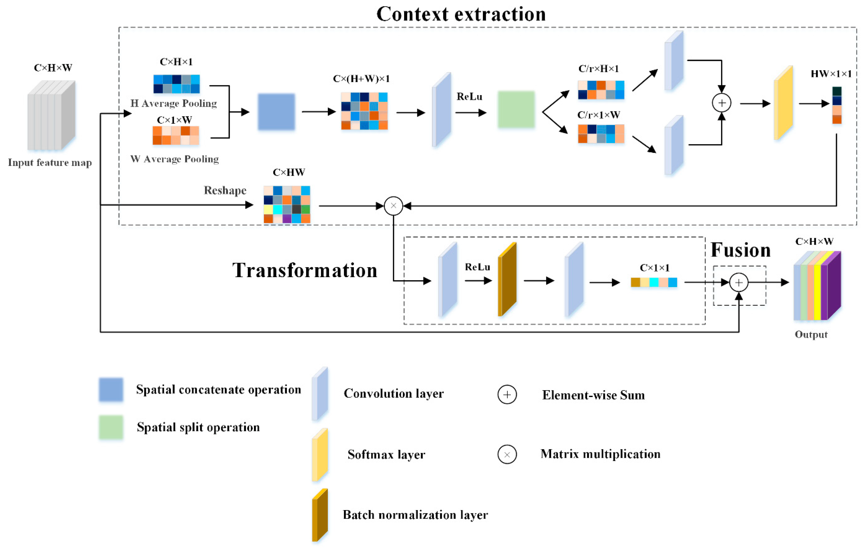
Ma et al. studied the classical attention module and established the framework of the attention module in a broad sense, thinking that the attention block is composed of three parts: context extraction, transformation, and fusion [37]. The structure of our designed attention block also conforms to this framework, as shown in Figure 2.
Context extraction is used to collect relevant feature information from the feature map of the internal relationship of the image. We assume that the feature map obtained by the previous convolution block is x C × H × W . We perform one-dimensional average pooling in two directions, so the outputs of the c -th channel at height h and width w are expressed as [34]
z c h = 1 W 0 i < W x c h , i
z c w = 1 H 0 j < H x c j , w
where C is the number of channels of the feature map, and H and W are the height and width of the feature map, respectively.
The above results in two independent orientation-aware feature maps, which not only capture the long-distance dependencies in their respective orientations well but also preserve spatial location information from each other.
Then z h and z w are used with convolution C o n v 1 to generate the aggregated feature map [34]:
f = δ C o n v 1 z h , z w
where
  • C o n v 1 is a convolutional layer with a convolution kernel size of 1 × 1 ,
  • · , · represents the connection operation along one dimension,
  • z h C × H × 1 and z w C × 1 × W are the input feature maps,
  • δ is the nonlinear activation function R e L u ,
  • f C / r × H + W × 1 is the output feature map,
  • r is a reduction ratio to reduce the amount of computation.
Then we cut it into separate tensors along the two spatial dimensions f h and f w . Then we use two convolutions C o n v 2 and C o n v 3 to restore the tensors as dimension C × H × W consistent with the input dimension. Finally, the two tensors are connected along the two spatial dimensions to form an attention map with long-distance dependencies initially:
G = C o n v 2 f h C o n v 3 f w
where C o n v 2 and C o n v 3 are convolutional layers with a convolution kernel size of 1 × 1 , respectively, indicates that the two matrices are added along different dimensions, f h C / r × H × 1 and f w C / r × 1 × W are the cut feature vectors, and G C × H × W is the generated attention map.
Unlike the coordinated attention module, the interaction between the attention map and the original image are used to calculate the position in the graph to capture long-range correlations after initially generating an attention map. Therefore, based on having a certain amount of attention, we further improve the context modeling ability, and aggregate the features of all positions to obtain global context features.
Inspired by [31], all pixels in the image share an attention map. The relationship between positions i and j can be expressed as
e i = j = 1 N e G x j p = 1 N e G x p x j
where N ( N equals H times W ) represents the total number of pixels in the image.
Transformation aims to capture the channel and space dependencies and transform the extracted features on the nonlinear attention space to obtain the attention map z f . The output z f can be expressed as [31]
z f = C o n v 5 δ B N C o n v 4 e i
where C o n v 4 and C o n v 5 are convolutional layers with a convolution kernel size of 1 × 1 , respectively, and δ represents the nonlinear activation function R e L U . B N represents batch normalization processing.
Fusion aims to combine the obtained attention map with the feature map of the original convolutional block. According to (2) to (7), the process of aggregating global context features into features of each location can be expressed as
z i = x i + C o n v 5 δ B N C o n v 4 e i
e i = j = 1 N e δ C o n v 1 z h , z w h δ C o n v 1 z h , z w w x j p = 1 N e δ C o n v 1 z h , z w h δ C o n v 1 z h , z w w x p x j
z c h = 1 W 0 i < W x c h , i
z c w = 1 H 0 j < H x c j , w
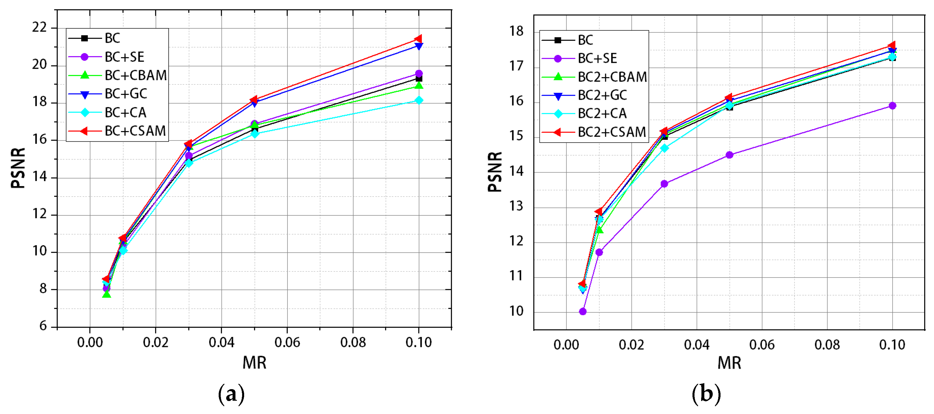
The attention module we designed not only acquires channel-level global features in the channel domain, but it also has a stronger ability to capture global information in the spatial domain. As mentioned above, we use the attention map in two directions to reflect whether there is a place to pay attention between the corresponding rows and columns, and then we encode the established attention map with itself. Then the global information is exploited to locate the areas that need attention accurately in the image. This enhances the power of context extraction and transformation nicely compared to general self-attention networks. Moreover, we also analyze the insufficiency of the global average pooling method in CSAM and propose an adaptive Gaussian filter to optimize this attention module (this is described in detail in the next section). Finally, the overall reconstruction ability of the network is improved. We showed this in experiments.

3.3. Adaptive Gaussian Filter Sub-Networks

Although the method of decomposing the 2D global average pooling into two parallel 1D feature encodings improves the ability of the network to utilize spatial information effectively in CSAM, Qin et al. pointed out that this method cannot capture rich input representation [38]. It was demonstrated that the global average pooling method is the lowest frequency component of the discrete cosine transform. In other words, in the frequency domain, only a single component is used, and other useful components are ignored. Usually, the low-frequency part of the image mainly contains general image information, while the high-frequency part mainly contains the detailed information of the image. These details are very important for the reconstruction of the image. So, an adaptive Gaussian filtering sub-network is proposed to solve this problem.
The specific implementation of two-dimensional Gaussian filtering assigns different Gaussian weight values to the surrounding pixel values within a certain range. It obtains the result of the current point after the weighted average. The two-dimensional Gaussian function is
G x , y = A e x x 0 2 2 σ x 2 + y y 0 2 2 σ y 2
where A is the amplitude, x 0 and y 0 are the center point coordinates, and σ x and σ y are the standard variances.
The amplitude of the two-dimensional Gaussian function is inversely proportional to the standard variances σ . The larger the σ , the wider the frequency band of the Gaussian filter and the better the smoothness. However, the two-dimensional Gaussian filter is mainly used as a controllable filter, so the amplitude is fixed to one.
Usually, the low-frequency part of the image mainly contains general image information, while the high-frequency part mainly contains detailed information of the image. When the measurement rate is lower, the compressed sampled image contains more low-frequency information, so the bandwidth of the filter can be set smaller when the measurement rate is higher. Therefore, the standard variances σ of the Gaussian filter sub-network we designed can vary with the measurement rate of the sampling network. In this way, the Gaussian filtering sub-network can supplement more frequency domain component information to the main network under different measurement rate conditions, which increases the expressive ability in the frequency domain. This method makes up for the deficiency of the global average pooling method and adopts the skip connection method as shown in Figure 1 to reduce the computational complexity.

3.4. AMLoss (Attention MSE Loss)

The MSE (mean square error) loss function has the advantages easily using the gradient descent algorithm and is conducive to the convergence of the function. However, the MSE loss function has the characteristics of giving a larger penalty to the larger error and a smaller penalty to the smaller error. If there are outliers in the sample, the MSE loss function will give higher weights to the outliers, thereby ignoring the influence of the image content itself, which will reduce the overall performance of the model ultimately. Although there are some works on the combination of attention and loss function [39,40,41], unfortunately, the combination of attention and MSE loss function is still very rare. Therefore, we propose an improved loss function based on the traditional MSE loss, which is called AMLoss (attention MSE loss). Its expression is
A M L o s s y ^ = α × 1 N i = 1 N y i ^ y i 2 + β × 1 N j = 1 N y j ^ y j 2
where N is the number of pixels in the image, α and β are the set hyperparameters, respectively, and y ^ and y ^ are the pixel values of the important area and the non-important area of the predicted value output y ^ by the network, respectively, y and y are the pixel values of the important area and the non-important area of the real value input y by the network, respectively.
In the training process, as shown in Figure 1, the designed adaptive grabbing module is used to extract its important area part before the input image enters the network. After that, it generates the corresponding important area mask matrix M I and unimportant area mask matrix M U . Finally, we multiply the predicted value y ^ and the real value y with the masks M I and M U to obtain the respective important and non-important regions. Take MNIST dataset as an example. The characteristic of this dataset is that the main part of the image is in the center of the image, and the value of pixels is very large. According to this feature, we design the capture module as follows: First, we normalize the image. Then we calculate the average pixel value of all pixels in the picture and compare the value of all pixels in the picture with the average pixel value. If the value of the pixel point is greater than the average pixel value, the position of the matrix corresponding to the point is assigned as 1. On the contrary, the position of the matrix corresponding to the point is assigned as 0. Finally, the important area matrix is generated. We believe that the important part of the image is determined according to the work task. If the important part of the picture is artificially defined, the method of extraction is not unitary. Different datasets also have different methods.
In this way, the MSE-loss function will increase the penalty for important areas of the image and reduce the penalty for non-important areas of the image. This will not only alleviate the defects of the above MSE-loss function but also make the loss function have “attention”, paying more attention to the important parts of the image. The error of the important part has a greater impact on the update of parameters such as weights and biases of the network after the back-propagation algorithm. The proof process is as follows:
The last activation function used by the last convolution of this network is L e a k y R e L U :
L e a k y R e L U z = z z > 0 γ z z 0
This function solves R e l u ’s neuron death problem with a small positive slope γ in negative regions, so it can backpropagate even for negative input values. We assume an input vector y , which is transformed by the L e a k y R e L U function to obtain a vector r , and propagates forward to obtain an error value e . We only solve the gradient of e to y and do not solve the update of specific parameters in the network after e backpropagation.
The known condition is:
y = y 1 , y 2 , y 3 , y 4 , , y n
r = L e a k y R e L U y
e = A M L o s s r
According to (11) and (13), we obtain:
d r i d y i = 1 y i > 0 γ y i 0
According to (13), the gradient of r to y is:
d r d y = d r 1 d y 1 , d r 2 d y 2 , d r 3 d y 3 , , d r n d y n
According to (10) and (14), the gradient of e to r is:
e r = e r 1 , e r 2 , e r 3 , , e r n = A M L o s s r r = α r 1 y 1 + β r 1 y 1 , α 2 r 2 y 2 + β 2 r 2 y 2 , α 3 r 3 y 3 + β 3 r 3 y 3 , , α n r n y n + β n r n y n
According to the chain rule, we obtain:
e y i = e r i d r i d y i
According to (16) and (18), the gradient of e to y is:
e y = e y 1 , e y 2 , e y 3 , , e y n = e r d r d y
where represents the multiplication of parity elements.
It can be seen from (19) that when α > 1 β , the weight of errors in important areas will be increased, and the weight of errors in non-important areas will remain the same or decrease. It is worth mentioning that the AMLoss is suitable for networks with an attention mechanism, because networks with an attention mechanism filter out important parts of the image. The AMLoss is more inclined to reduce the loss value for important parts of the image when it is minimized by backpropagation.

4. Experiments and Results

In this section, we design three experiments to test the reconstruction performance of the ACRM. They are a comparison of different attention mechanism modules, an optimization comparison of the AMLoss in different attention mechanism networks, and a comparison of different compressed sensing networks. Our experiments were implemented in the TensorFlow 2.0 framework and run on CUDA11 for accelerated processing. The computer we used was equipped with an Intel Xeon W-2133 CPU, an Nvidia GEFORCE RTX 2080Ti 11GB graphics card (in particular, we used Nvidia RTX A6000 48G for CelebA dataset), 64 GB of RAM, and a 2 T hard drive. The configuration of specific network parameters is explained in the following subsections.

4.1. Comparison of Different Attention Mechanism Modules

The feature-rich MNIST handwriting dataset and Fashion-MNIST dataset were used as training data. Taking the Fashion-MNIST dataset as an example, 40,000 images and 10,000 images were selected as training and testing sets, respectively, according to the hold-out method. The batch size of each entry into the network was 64. Each training was 500 batches. One round of training was 32,000 pictures. Total training was 100 rounds. The optimizer chose ADAM, and the learning rate was set to 10 4 . We tested with images from the test set and calculated the average of the metrics.
In this experiment, the main purpose was to verify the improvement effect of the attention mechanism module on the reconstruction ability of the general compressed sensing network. We compared the CSAM with the classical attention mechanism module to verify the superiority of that in the compression reconstruction network. To highlight the superiority of the attention module, we simplified the convolutional network in the ACRM and built a basic convolutional network (BC-Net) consisting of two fully connected layers and eight convolutional connections as the main network. The eight convolution kernels were divided into four BC modules, and each group of BC modules was composed of convolution kernel size and channel number of 11 × 11 × 64 and 7 × 7 × 1, respectively. The L e a k y R e L U function was used after each convolutional layer. The SE-Net [32], the CBAM [42], the coordinated attention module [34], and the GC-Net [31] were embedded in it, respectively, as shown in Figure 3. The modules surrounded by dotted lines in Figure 3 were used to place different attention mechanism modules in the experiments. At the same time, we also set up a group of ablation experiments to verify the effectiveness of the sub network. The dataset adopted fashion MNIST, and the network and dataset settings were consistent with the above. Finally, all networks used the general MSE function as the loss function. The signal-to-noise ratio (PSNR) and structural similarity (SSIM) were used as evaluation metrics for reconstruction performance. The calculation formulas of PSNR and SSIM are as follows:
P S N R = 10 × log 10 255 2 M S E
M S E = 1 H W i = 0 H 1 j = 0 W 1 | X i , j Y i , j | 2
S S I M X , Y = 2 μ X μ Y + c 1 2 σ X Y + c 2 μ Y 2 + μ Y 2 + c 1 σ X 2 + σ Y 2 + c 2
where H and W are the height and width of the image, respectively, and MSE represents the mean square error of the current image X and the reference image Y. μ X and μ Y are the mean of X and Y , respectively, σ X and σ Y are the variances of X and Y , respectively, σ X Y is the covariance of X and Y , and c 1 and c 2 are constants.
The experimental results are shown in Table 1 and Table 2. The measurement rate (MR) is the ratio M / N of the sampling points M of the image to the total image pixels N . The CSAM outperformed in all comparisons from the table. The PSNR at all measurement rates was better than the other networks. It can be seen from Table 3 that under different measurement rates, the reconstruction effect was improved by using the adaptive Gaussian filter sub network, which proved the effectiveness of the sub network. Figure 4 shows the differences in the PSNR values of several models under different datasets. Other attention modules cannot maintain consistent performance in different datasets, which indicates that the CSAM is more robust than other attention modules.

4.2. Optimization Comparison of the AMLoss in Different Attention Mechanism Networks

In this subsection, we designed five sets of controlled experiments to verify that the AMLoss can optimize the compressed sensing network with an attention mechanism. The backbone network of this experiment used the BC-Net proposed in the previous section. The configuration of training parameters was the same as in the previous section. In this experiment, only the MNIST dataset was used for experiments. A set of controlled experiments was set up for each network, which were trained using the MSE-Loss and the AMLoss as loss functions, respectively. We tested with images from the test set and calculated the average of the metrics.
The experimental results are shown in Table 4. The AMLoss could improve the attention compressed sensing network significantly when we chose a suitable α. This boost was most pronounced at higher measurement rates. Figure 5 also shows that the reconstructed image using the AMLoss network contained more detail and less noise. The above experiments showed that the loss function with attention could help the network to pay more attention to the important part during the training process and add more details to the part. Finally, the overall quality of the reconstructed image was improved.

4.3. Comparison of Different Compressed Sensing Networks

In this subsection, we compared ACRM with other algorithms and demonstrated the advantages of our network in reconstruction tasks. In this experiment, the Fashion-MNIST and CelebA datasets were used as datasets. For the Fashion-MNIST dataset, our parameter settings were the same as in the first subsection. For the CelebA dataset, scaled and cropped to a standard size of 64 × 64 , 200,000 images and 700 images were selected as training and test sets, respectively. The batch size of each entry into the network was 64. Each training was 3125 batches. Total training was 20 rounds. Regardless of the dataset used, we tested with images from the test set and calculated the average of the metrics. A simulated sampling network (FC layer) was added to all the networks used for comparison to ensure the fairness of the experiments. Related work proved that this method improves the image reconstruction accuracy of the network [36], so our modification did not affect the performance of the original network. The networks used for comparison in the experiments were Recon-Net [16], DR2-Net [17], and Bsr2-Net [43].
The experimental results are shown in Table 5 and Table 6. The ACRM achieved the highest PSNR and SSIM values among all comparative experiments. Figure 6 shows the PSNR difference and loss convergence for each reconstruction model under different datasets. Figure 6 and Figure 7 show the reconstruction samples of different reconstruction networks. They show that ACRM improved the learning ability and expressive ability of the network. In addition, it can be seen from (b) and (d) in Figure 6 that the ACRM had good efficiency on different datasets. Although the decline rate of loss in the early stage was slightly lower than that of Recon-Net, it overtook Recon-Net in the later stage.

5. Conclusions

In this study, we propose a deep learning-based compressed sensing network (ACRM) for single-pixel imaging. The ACRM combines a coordinated self-attention mechanism and uses an adaptive Gaussian filtering method to make up for the insufficiency of global average pooling. Then, the AMLoss, which incorporates attention ideas, is used for optimization. A series of experiments shows that the combination of the CSAM and adaptive Gaussian filter can fully utilize the global spatial information and channel information. Compared with the traditional compressed sensing neural network, the ACRM has a better reconstruction effect and reconstruction accuracy. It retains rich semantic information and has good network efficiency at a low measurement rate. It performs well in different datasets, indicating its strong robustness. After theoretical and experimental demonstrations, the AMLoss has a better reconstruction effect for the attention mechanism.

Author Contributions

Conceptualization, Z.W., Q.Y. and X.L.; Methodology, Z.W., Q.Y. and Y.Z.; Software, Z.W., Y.Z., S.S. and J.L.; Validation, Z.W., Y.Z., S.S. and J.L.; Formal analysis, Z.W., Q.Y., S.S. and J.L.; Investigation, Z.W., Q.Y., X.L., S.S. and J.L.; Resources, Q.Y. and X.L.; Data curation, Z.W. and Q.Y.; Writing—original draft, Z.W.; Writing—review & editing, Z.W. and Q.Y.; Visualization, Z.W.; Supervision, Q.Y., X.L. and Y.Z.; Project administration, Q.Y. and X.L.; Funding acquisition, Q.Y. All authors have read and agreed to the published version of the manuscript.

Funding

This research was funded by National Natural Science Foundation of China grant number No. 62165009.

Data Availability Statement

Not applicable.

Conflicts of Interest

The authors declare no conflict of interest.

References

  1. Kasin, B. The widths of certain finite-dimensional sets and classes of smooth functions. Izv. Akad. Nauk SSSR Ser. Mat. 1977, 41, 334–351. [Google Scholar]
  2. Candes, E.; Romberg, J. Sparsity and incoherence in compressive sampling. Inverse Probl. 2007, 23, 969. [Google Scholar] [CrossRef]
  3. Donoho, D.L. Compressed sensing. IEEE Trans. Inf. Theory 2006, 52, 1289–1306. [Google Scholar] [CrossRef]
  4. Tsaig, Y.; Donoho, D.L. Extensions of compressed sensing. Signal Process. 2006, 86, 549–571. [Google Scholar] [CrossRef]
  5. Candès, E.J. Compressive sampling. In Proceedings of the International Congress of Mathematicians, Madrid, Spain, 22–30 August 2006; pp. 1433–1452. [Google Scholar]
  6. Candès, E.J.; Wakin, M.B. An introduction to compressive sampling. IEEE Signal Process. Mag. 2008, 25, 21–30. [Google Scholar] [CrossRef]
  7. Duarte, M.F.; Davenport, M.A.; Takhar, D.; Laska, J.N.; Sun, T.; Kelly, K.F.; Baraniuk, R.G. Single-pixel imaging via compressive sampling. IEEE Signal Process. Mag. 2008, 25, 83–91. [Google Scholar] [CrossRef]
  8. Li, W.; Hu, X.; Wu, J.; Fan, K.; Chen, B.; Zhang, C.; Hu, W.; Cao, X.; Jin, B.; Lu, Y. Dual-color terahertz spatial light modulator for single-pixel imaging. Light Sci. Appl. 2022, 11, 191. [Google Scholar] [CrossRef]
  9. Lin, J.; Yan, Q.; Lu, S.; Zheng, Y.; Sun, S.; Wei, Z. A Compressed Reconstruction Network Combining Deep Image Prior and Autoencoding Priors for Single-Pixel Imaging. Photonics 2022, 9, 343. [Google Scholar] [CrossRef]
  10. Lustig, M.; Donoho, D.L.; Santos, J.M.; Pauly, J.M. Compressed sensing MRI. IEEE Signal Process. Mag. 2008, 25, 72–82. [Google Scholar] [CrossRef]
  11. Vasudeva, B.; Deora, P.; Bhattacharya, S.; Pradhan, P.M. Compressed Sensing MRI Reconstruction with Co-VeGAN: Complex-Valued Generative Adversarial Network. In Proceedings of the IEEE/CVF Winter Conference on Applications of Computer Vision, Waikoloa, HI, USA, 4–8 January 2022; pp. 672–681. [Google Scholar]
  12. Liu, X.-J.; Xia, S.-T.; Fu, F.-W. Reconstruction guarantee analysis of basis pursuit for binary measurement matrices in compressed sensing. IEEE Trans. Inf. Theory 2017, 63, 2922–2932. [Google Scholar] [CrossRef]
  13. Nguyen, N.; Needell, D.; Woolf, T. Linear convergence of stochastic iterative greedy algorithms with sparse constraints. IEEE Trans. Inf. Theory 2017, 63, 6869–6895. [Google Scholar] [CrossRef]
  14. Candès, E.J.; Romberg, J.; Tao, T. Robust uncertainty principles: Exact signal reconstruction from highly incomplete frequency information. IEEE Trans. Inf. Theory 2006, 52, 489–509. [Google Scholar] [CrossRef]
  15. Li, C.; Yin, W.; Jiang, H.; Zhang, Y. An efficient augmented Lagrangian method with applications to total variation minimization. Comput. Optim. Appl. 2013, 56, 507–530. [Google Scholar] [CrossRef]
  16. Kulkarni, K.; Lohit, S.; Turaga, P.; Kerviche, R.; Ashok, A. Reconnet: Non-iterative reconstruction of images from compressively sensed measurements. In Proceedings of the IEEE Conference on Computer Vision and Pattern Recognition, Las Vegas, NV, USA, 27–30 June 2016; pp. 449–458. [Google Scholar]
  17. Yao, H.; Dai, F.; Zhang, S.; Zhang, Y.; Tian, Q.; Xu, C. Dr2-net: Deep residual reconstruction network for image compressive sensing. Neurocomputing 2019, 359, 483–493. [Google Scholar] [CrossRef]
  18. Babacan, S.D.; Molina, R.; Katsaggelos, A.K. Bayesian compressive sensing using Laplace priors. IEEE Trans. Image Process. 2009, 19, 53–63. [Google Scholar] [CrossRef]
  19. Mousavi, A.; Patel, A.B.; Baraniuk, R.G. A deep learning approach to structured signal recovery. In Proceedings of the 2015 53rd Annual Allerton Conference on Communication, Control, and Computing (Allerton), Monticello, IL, USA, 29 September–2 October 2015; pp. 1336–1343. [Google Scholar]
  20. Mousavi, A.; Baraniuk, R.G. Learning to invert: Signal recovery via deep convolutional networks. In Proceedings of the 2017 IEEE International Conference on Acoustics, Speech and Signal Processing (ICASSP), New Orleans, LA, USA, 5–9 March 2017; pp. 2272–2276. [Google Scholar]
  21. Lohit, S.; Kulkarni, K.; Kerviche, R.; Turaga, P.; Ashok, A. Convolutional neural networks for noniterative reconstruction of compressively sensed images. IEEE Trans. Comput. Imaging 2018, 4, 326–340. [Google Scholar] [CrossRef]
  22. Yang, Y.; Sun, J.; Li, H.; Xu, Z. ADMM-CSNet: A deep learning approach for image compressive sensing. IEEE Trans. Pattern Anal. Mach. Intell. 2018, 42, 521–538. [Google Scholar] [CrossRef]
  23. Yuan, Z.; Jiang, M.; Wang, Y.; Wei, B.; Li, Y.; Wang, P.; Menpes-Smith, W.; Niu, Z.; Yang, G. SARA-GAN: Self-attention and relative average discriminator based generative adversarial networks for fast compressed sensing MRI reconstruction. Front. Neuroinform. 2020, 14, 611666. [Google Scholar] [CrossRef]
  24. Zhang, X.; Wu, X. Attention-guided image compression by deep reconstruction of compressive sensed saliency skeleton. In Proceedings of the IEEE/CVF Conference on Computer Vision and Pattern Recognition, Nashville, TN, USA, 19–25 June 2021; pp. 13354–13364. [Google Scholar]
  25. Barranca, V.J. Neural network learning of improved compressive sensing sampling and receptive field structure. Neurocomputing 2021, 455, 368–378. [Google Scholar] [CrossRef]
  26. Hayhoe, M.; Ballard, D. Eye movements in natural behavior. Trends Cogn. Sci. 2005, 9, 188–194. [Google Scholar] [CrossRef]
  27. Guo, M.-H.; Xu, T.-X.; Liu, J.-J.; Liu, Z.-N.; Jiang, P.-T.; Mu, T.-J.; Zhang, S.-H.; Martin, R.R.; Cheng, M.-M.; Hu, S.-M. Attention mechanisms in computer vision: A survey. Comput. Vis. Media 2022, 8, 331–368. [Google Scholar] [CrossRef]
  28. Zheng, X.; Wang, B.; Du, X.; Lu, X. Mutual attention inception network for remote sensing visual question answering. IEEE Trans. Geosci. Remote Sens. 2021, 60, 5606514. [Google Scholar] [CrossRef]
  29. Zheng, X.; Chen, W.; Lu, X. Spectral super-resolution of multispectral images using spatial–spectral residual attention network. IEEE Trans. Geosci. Remote Sens. 2021, 60, 5404114. [Google Scholar] [CrossRef]
  30. Wang, X.; Girshick, R.; Gupta, A.; He, K. Non-local neural networks. In Proceedings of the IEEE Conference on Computer Vision and Pattern Recognition, Salt Lake City, UT, USA, 18–23 June 2018; pp. 7794–7803. [Google Scholar]
  31. Cao, Y.; Xu, J.; Lin, S.; Wei, F.; Hu, H. Gcnet: Non-local networks meet squeeze-excitation networks and beyond. In Proceedings of the IEEE/CVF International Conference on Computer Vision Workshops, Seoul, Republic of Korea, 27–28 October 2019. [Google Scholar]
  32. Hu, J.; Shen, L.; Sun, G. Squeeze-and-excitation networks. In Proceedings of the IEEE Conference on Computer Vision and Pattern Recognition, Salt Lake City, UT, USA, 18–23 June 2018; pp. 7132–7141. [Google Scholar]
  33. Wang, Q.; Wu, B.; Zhu, P.; Li, P.; Hu, Q. ECA-Net: Efficient Channel Attention for Deep Convolutional Neural Networks. In Proceedings of the 2020 IEEE/CVF Conference on Computer Vision and Pattern Recognition (CVPR), Seattle, WA, USA, 13–19 June 2020. [Google Scholar]
  34. Hou, Q.; Zhou, D.; Feng, J. Coordinate attention for efficient mobile network design. In Proceedings of the IEEE/CVF Conference on Computer Vision and Pattern Recognition, Nashville, TN, USA, 20–25 June 2021; pp. 13713–13722. [Google Scholar]
  35. Vaswani, A.; Shazeer, N.; Parmar, N.; Uszkoreit, J.; Jones, L.; Gomez, A.N.; Kaiser, Ł.; Polosukhin, I. Attention is all you need. Adv. Neural Inf. Process. Syst. 2017, 30, 3258. [Google Scholar]
  36. Guan, Y.; Yan, Q.; Yang, S.; Li, B.; Cao, Q.; Fang, Z. Single photon counting compressive imaging based on a sampling and reconstruction integrated deep network. Opt. Commun. 2020, 459, 124923. [Google Scholar] [CrossRef]
  37. Ma, X.; Guo, J.; Tang, S.; Qiao, Z.; Chen, Q.; Yang, Q.; Fu, S. DCANet: Learning connected attentions for convolutional neural networks. arXiv 2020, arXiv:2007.05099. [Google Scholar]
  38. Qin, Z.; Zhang, P.; Wu, F.; Li, X. Fcanet: Frequency channel attention networks. In Proceedings of the IEEE/CVF International Conference on Computer Vision, Montreal, BC, Canada, 11–17 October 2021; pp. 783–792. [Google Scholar]
  39. Abraham, N.; Khan, N.M. A novel focal tversky loss function with improved attention u-net for lesion segmentation. In Proceedings of the 2019 IEEE 16th International Symposium on Biomedical Imaging (ISBI 2019), Venice, Italy, 8–11 April 2019; pp. 683–687. [Google Scholar]
  40. Wang, W.; Su, C. Convolutional neural network-based pavement crack segmentation using pyramid attention network. IEEE Access 2020, 8, 206548–206558. [Google Scholar] [CrossRef]
  41. Yu, J.; Wu, B. Attention and hybrid loss guided deep learning for consecutively missing seismic data reconstruction. IEEE Trans. Geosci. Remote Sens. 2021, 60, 5902108. [Google Scholar] [CrossRef]
  42. Woo, S.; Park, J.; Lee, J.-Y.; Kweon, I.S. Cbam: Convolutional block attention module. In Proceedings of the European conference on computer vision (ECCV), Munich, Germany, 8–14 September 2018; pp. 3–19. [Google Scholar]
  43. Li, B.; Yan, Q.-R.; Wang, Y.-F.; Yang, Y.-B.; Wang, Y.-H. A binary sampling Res2net reconstruction network for single-pixel imaging. Rev. Sci. Instrum. 2020, 91, 033709. [Google Scholar] [CrossRef]
Figure 1. ACRM structure diagram. It contains 2 fully connected layers, 4 CSAMs, 12 convolutional layers, and an adaptive Gaussian filter. Each CSAM module and 3 convolutions make up the ACR submodule. The kernel sizes and channels of the three convolutional layers from left to right are 11 × 11 × 64, 7 × 7 × 32, and 3 × 3 × 1, respectively. In addition to sequential connections between each module, there are skip connections. The grab module generates the corresponding important area mask matrix M I and unimportant area mask matrix M U . Then, we multiply the y ^ and y with the M I and M U to obtain y , y , y ^ , and y ^ . Finally, the AMLoss for backpropagation optimization is obtained.
Mathematics 11 00847 g001
Figure 2. CSAM structure diagram. The module contains three parts: context extraction, transformation, and fusion. Among them, “H Average Pooling” and “W Average Pooling” refer to 1D horizontal average pooling and 1D vertical average pooling, respectively. “ReLu” is the nonlinear activation function ReLu; “r” is a reduction ratio to reduce the amount of computation.
Mathematics 11 00847 g002
Figure 3. The structure diagram of BC-Net. It contains 2 fully connected layers and 8 convolutional layers. The 8 convolutional layers form 4 BC modules. In addition to the sequential connections between each module, there are skip connections. After the first convolutional layer of each module, the attention mechanism modules can be connected sequentially to form an attention-compressed sensing network.
Mathematics 11 00847 g003
Figure 4. (a) Different attention mechanism algorithms test the PSNR of MNIST pictures at different measurement rates. (b) Different attention mechanism algorithms test the PSNR of Fashion-MNIST pictures at different measurement rates.
Mathematics 11 00847 g004
Figure 5. Model images were reconstructed on the MNIST dataset, MR = 0.01. The top-down compressed sensing networks are (a) BC + SE, (b) BC + CBAM, (c) BC + GC, (d) BC + CA, and (e) BC + CSAM.
Mathematics 11 00847 g005
Figure 6. (a) PSNR of different algorithms at different measurement rates on the Fashion-MNIST dataset. (b) Loss values of test images of different algorithms on the Fashion-MNIST dataset. (c) PSNR of different algorithms at different measurement rates on the CelebA dataset. (d) Loss values of test images of different algorithms on the CelebA dataset.
Mathematics 11 00847 g006
Figure 7. Model images are reconstructed on the CelebA dataset, MR = 0.1. From top to bottom are the (a) original image, (b) Recon-Net reconstructed image, (c) DR2-Net reconstructed image, (d) Bsr2-Net reconstructed image, and (e) ACRM reconstructed image.
Mathematics 11 00847 g007
Table 1. PSNR and SSIM of algorithms embedded with different attention mechanisms on the MNIST dataset at different measurement rates.
MethodsMR = 0.1MR = 0.05MR = 0.03MR = 0.01MR = 0.005
PSNRSSIMPSNRSSIMPSNRSSIMPSNRSSIMPSNRSSIM
BC19.3440.92516.6190.85914.9640.79810.5630.5788.2880.364
BC + SE19.5910.93216.8940.88215.1950.82110.3320.5618.4120.381
BC + CBAM18.9180.87916.8190.8615.6580.84210.5990.5577.7370.294
BC + GC21.0910.95318.0430.91215.6520.84410.6790.5848.4990.382
BC + CA18.150.8916.3620.84514.7880.7810.110.5248.4460.39
BC + CSAM21.4480.95318.1990.9215.8360.85610.7890.5958.5920.416
Note: Bold numbers indicate the best value for that measurement.
Table 2. PSNR and SSIM of algorithms embedded with different attention mechanisms on the Fashion-MNIST dataset at different measurement rates.
MethodsMR = 0.1MR = 0.05MR = 0.03MR = 0.01MR = 0.005
PSNRSSIMPSNRSSIMPSNRSSIMPSNRSSIMPSNRSSIM
BC17.2840.76915.880.71815.0310.67812.6860.56310.7290.428
BC + SE17.4120.78215.8570.72314.9470.68512.5840.55110.4930.409
BC + CBAM17.4930.79215.9470.73115.0930.68712.340.54310.790.453
BC + GC17.4810.78716.0530.72915.1370.68912.6530.56810.6650.42
BC + CA17.3030.78415.9240.72614.6950.65912.6570.55610.8050.441
BC + CSAM17.6360.79116.1510.73915.1830.68912.8850.65610.8210.45
Note: Bold numbers indicate the best value for that measurement.
Table 3. Ablation study on the adaptive Gaussian filter (AGF).
MethodsMR = 0.1MR = 0.05MR = 0.03MR = 0.01MR = 0.005
PSNRSSIMPSNRSSIMPSNRSSIMPSNRSSIMPSNRSSIM
BC + CSAM17.6360.79116.1510.73915.1830.68912.8850.65610.8210.45
BC + CSAM + AGF17.9640.80216.3340.75215.2310.70212.9750.67510.8940.47
σ = 6 σ = 6 σ = 5 σ = 2.75 σ = 1
Note: Bold numbers indicate the best value for that measurement. σ is the standard variance of the Gaussian filter at different measurement rates.
Table 4. Performance comparison of the AMLoss and MSE-Loss acting on different attention compressed sensing networks in the MNIST dataset.
MethodsLossMR = 0.1MR = 0.05MR = 0.03MR = 0.01MR = 0.005
PSNRSSIMPSNRSSIMPSNRSSIMPSNRSSIMPSNRSSIM
BC + SEMSE-Loss19.5910.93216.8940.88215.1950.82110.3320.5618.4120.381
AMLoss (2)20.8140.94317.6010.89415.2230.82110.5030.5648.5290.382
BC + CBAMMSE-Loss18.9180.87916.8190.8615.6580.84210.5990.5577.7370.294
AMLoss (1.1)21.0420.95317.5120.89415.8240.84510.7210.5598.320.404
BC + GCMSE-Loss21.0910.95318.0430.91215.6520.84410.6790.5848.4990.382
AMLoss (1.2)21.2100.95518.2440.9215.7390.84510.7580.5888.5530.386
BC + CAMSE-Loss18.150.8916.3620.84514.7880.7810.110.5248.4460.39
AMLoss (1.2)20.3950.94417.60.90915.0420.82210.240.5718.5210.41
BC + CSAMMSE-Loss21.4480.95318.1990.9215.8360.85610.7890.5958.5920.416
AMLoss (1.15)22.1820.95918.4850.93116.120.8610.8470.6058.6460.418
Note: The bold numbers represent the best value for a network at that measurement rate. The value in parentheses next to “AMLoss” is the value of α ( β is 1 by default).
Table 5. PSNR and SSIM of different algorithms are performed on the Fashion-MNIST dataset with different measurement rates.
MethodsMR = 0.1MR = 0.05MR = 0.03MR = 0.01
PSNRSSIMPSNRSSIMPSNRSSIMPSNRSSIM
Recon-Net17.6010.79615.0390.69314.370.63912.0940.519
DR2-Net17.7840.80415.9560.7215.0460.68312.7410.56
Bsr2-Net17.8850.79616.3040.74915.3570.69513.2610.598
ACRM (1.1)18.120.81716.6730.75715.7430.71913.4380.603
σ = 6 σ = 6 σ = 4.75 σ = 4
Note: Bold numbers indicate the best value at that sample rate. The value in parentheses next to “ACRM” is the value of α ( β is 1 by default); σ is the standard variance of the Gaussian filter.
Table 6. PSNR and SSIM of different algorithms are performed on the CelebA dataset with different measurement rates.
MethodsMR = 0.1MR = 0.05MR = 0.03MR = 0.01
PSNRSSIMPSNRSSIMPSNRSSIMPSNRSSIM
Recon-Net22.3470.84320.5070.76418.910.68116.1360.524
DR2-Net20.8930.77619.6020.71218.490.65115.9490.509
Bsr2-Net20.8330.77219.8340.72618.7270.66915.9690.51
ACRM (1.2)22.380.84320.5430.76719.0270.6916.1880.535
σ = 7 σ = 6 σ = 5.75 σ = 2
Note: Bold numbers indicate the best value at that sample rate. The value in parentheses next to “ACRM” is the value of α ( β is 1 by default); σ is the standard variance of the Gaussian filter.
Disclaimer/Publisher’s Note: The statements, opinions and data contained in all publications are solely those of the individual author(s) and contributor(s) and not of MDPI and/or the editor(s). MDPI and/or the editor(s) disclaim responsibility for any injury to people or property resulting from any ideas, methods, instructions or products referred to in the content.

