Topological Regularization for Representation Learning via Persistent Homology

Abstract

Generalization is challenging in small-sample-size regimes with over-parameterized deep neural networks, and a better representation is generally beneficial for generalization. In this paper, we present a novel method for controlling the internal representation of deep neural networks from a topological perspective. Leveraging the power of topology data analysis (TDA), we study the push-forward probability measure induced by the feature extractor, and we formulate a notion of “separation” to characterize a property of this measure in terms of persistent homology for the first time. Moreover, we perform a theoretical analysis of this property and prove that enforcing this property leads to better generalization. To impose this property, we propose a novel weight function to extract topological information, and we introduce a new regularizer including three items to guide the representation learning in a topology-aware manner. Experimental results in the point cloud optimization task show that our method is effective and powerful. Furthermore, results in the image classification task show that our method outperforms the previous methods by a significant margin.

1. Introduction

Although over-parameterized deep neural networks generalize well in practice when sufficient data are provided, in small-sample-size regimes, generalization is more difficult and requires careful consideration. Since the ability to learn task-specific representations is beneficial for generalization, a lot of effort has been dedicated to imposing structure on the latent space or representation space via additional regularizers [1,2], to guide the mapping from input space into internal space, or control properties of the internal representations [3]. However, internal representations are high-dimensional, discrete, sparse, incomplete and noisy; extraction of information from this kind of data is rather challenging.

In order to explore and control internal representations, there are various ways to choose: (1) For the algebraic methods based on vector space [4], coordinates are not natural, the power of linear transformation is limited, and low-dimensional visualizations cannot faithfully characterize the data. (2) For the statistical methods [5], a small sample size limits the power of the analysis, inference and computation; asymptotic statistics cannot be used; and the results may exhibit large variance. (3) For geometric methods based on distances [6] or manifold assumptions [7], it is difficult to capture the global picture, and metrics are not theoretically justified [8] (for neural networks, notions of distance are constructed by the feature extractor, which is hard to understand). Individual parameter choices may significantly influence the results, and constraints based on geometry information, such as pairwise distances, may be too strict to respect reality. (4) Methods based on calculus [9,10] can capture the local information in a small neighborhood for each point, but the performance is questionable while high-dimensional data are sparse and the sample size is small.

Besides the above traditional methods, there is another fundamentally different perspective, an unexplored, powerful tool to employ, i.e., the topological data analysis (TDA) method. The advantages of TDA methods [8,11,12,13] are as follows: (1) TDA studies the global “shape” of data and explores the underlying topological and geometric structures of point clouds. As a complement to localized and generally more rigid geometric features, topological features are suitable for capturing multi-scale, global and intrinsic properties of data. (2) Topology methods study geometric features in a way that is less sensitive to the choice of metrics, and this insensitivity is beneficial when the metric is not well understood or only determined in a coarse way [8], as in the neural networks. (3) Topology methods are coordinate-free, and they only focus on the intrinsic geometric properties of the geometric objects. (4) Instead of determining a proper spatial scale to understand and control the data, persistent homology collects information over the whole domains of parameter values and creates a summary in which the features that persist over a wide range of spatial scales are considered more likely to represent true features of the underlying space rather than artifacts of sampling, noise or particular choice of parameters.

1.1. Related Works

Previous work related to our work can be divided into two categories. The first category focuses on regularization using statistical information of internal representations. Cogswell et al. [1] proposed a regularizer to encourage diverse or non-redundant representations by minimizing the cross-covariance of internal representation. Choi et al. [2] designed two class-wise regularizers to enforce the desired characteristic for each class; one focused on reducing the covariance of the representations for samples from the same class, and the other used variance instead of covariance to improve compactness. The second category studies deep neural networks using tools from algebraic topology, in particular, persistent homology. Brüel-Gabrielsson et al. [14] presented a differentiable topology layer to extract topological features, which can be used to promote topological structure or incorporate a topological prior via regularization. Kim et al. [15] proposed a topological layer for generative deep models to feed critical topological information into subsequent layers and provided an adaptation for the distance-to-measure (DTM) function-based filtration. Hajij et al. [16] defined and studied the classification problem in machine learning in a topological setting and showed when the classification problem is possible or not possible in the context of neural networks. Li et al. [17] proposed an active learning algorithm to characterize the decision boundaries using their homology. Chen et al. [18] proposed measuring the complexity of the classification boundary via persistent homology, and the topological complexity was used to control the decision boundary via regularization. Vandaele et al. [19] introduced a novel set of topological losses to topologically regularize data embeddings in unsupervised feature learning, which can efficiently incorporate a topological prior. Hofer et al. [20] considered the problem of representation learning, treated each mini-batch as a point cloud, and controlled the connectivity of latent space via a novel topological loss. Moor et al. [3] extended this work and proposed a loss term to harmonize the topological features of the input space with the topological features of the latent space. This approach also acts on the level of mini-batches, computes persistence diagrams for both input space and latent space, and encourages these two persistence diagrams (PD) to be similar by the regularization item. Wu et al. [21] explored the rich spatial behavior of data in the latent space, proposed a topological filter to filter out noisy labels, and theoretically proved that the method is guaranteed to collect clean data with high probability. These works show empirically or theoretically that enforcing a certain topological structure on representation space can be beneficial for learning tasks.

Hofer et al. [22] proposed an approach to regularize the internal representation to control the topological properties of the internal space, and proved that this approach would enforce mass concentration effects which are beneficial for generalization. However, the authors based their work on the assumption that a loss function that yields a large margin in the representation space should be selected and, therefore, that the mass concentration effect is only beneficial if the reference set is located sufficiently far away from the decision boundary, but this large margin assumption may be violated in practice.

1.2. Contribution

In this paper, we apply the TDA method, in particular, persistent homology from algebraic topology, to analyze and control the global topology of the internal representations of the training points, which reveals the intrinsic structure of the representation space.

When TDA is combined with statistics, data are deemed to be generated from some unknown distribution instead of some underlying manifold. TDA methods are used to infer topological features of the underlying distribution, especially the support of the dis-tribution. Inspired by [22], by combining statistics with topological data analysis, our work focuses on the probability measure induced by the feature extractor and treats the representation of the training points in a mini-batch as point cloud data from which the topological information is extracted, and then we compute persistence diagram of the persistent homology. Specifically, we consider the topological properties of the samples from the product measure of two classes to enforce intra-class mass concentration and separation between classes simultaneously. We extend the definitions and techniques in [22] to formalize the separation between two classes via persistent homology. We argue that if this separation property is encouraged, then both mass concentration and separation will be enforced, and we proposed a novel weight function and constructed a novel loss to control the topological properties of the representation space.

In summary, our contributions are as follows:

(1) We characterize a separation property between two classes in representation space in terms of persistent homology (Section 3.2).

(2) We prove that a topological constraint on the samples of the push-forward probability measure in the presentation space leads to mass separation (Section 3.2).

(3) We propose a novel weight function based on DTM. Using our weight function, the weighted Rips filtration can be built on top of training samples from class pairs in a mini-batch. The stability of the persistence diagram with respect to the proposed weight function is presented (Section 3.4).

(4) We propose three regularization items, including a birth loss, a margin loss and a length loss, which operate on a persistence diagram obtained via persistent homology computations on mini-batches, to encourage mass separation (Section 3.4).

The remainder of this paper is structured as follows: In Section 2, we present some topological preliminaries relevant to our work. Section 3 gives our main results, including the separation property, the weight function and the regularization method. Section 4 shows the experimental results on synthetic data and benchmark datasets. Finally, Section 5 gives the conclusion.

2. Topological Preliminaries

Generally, in topological data analysis, the point clouds are thought to be finite samples taken from an underlying geometric object. To extract topological and geometric information, a natural way is to “connect” data points that are close to each other to build a global continuous shape on top of the data. This section contains a brief introduction to the relevant topological notions. More details can be found in several excellent introductions and surveys [8,11,12,13,23].

2.1. Simplicial Complex, Persistent Homology and Persistence Diagrams

Simplicial complex K is a discrete structure built over a finite set of samples to provide a topological approximation of the underlying topology or geometry. The Čech complex and the Vietoris-Rips complex are widely used in TDA. Below, for any $x\in \mathcal{X}$ and $r>0$, let $B(x;r)$ be the open ball of radius $r>0$ centered at $x$.

Definition 1 

(Čech complex [11]). Let $X\subset \mathcal{X}$ be finite and $r>0$. The Čech complex $\mathcal{C}(X;r)$ is the simplicial complex

$$\{x_0,\dots ,x_k\}\in \mathcal{C}(X;r):\iff \underset{i=0}{\overset{k}{\cap }}\overline{B}(x_i;r)\ne \varnothing$$

(1)

Definition 2 

(Vietoris-Rips complex [11]). Let $X\subset \mathcal{X}$ be finite and r > 0. The Vietoris-Rips complex $\mathcal{R}(X;r)$ is the simplicial complex

$$\begin{array}{c}\{x_0,\dots ,x_k\}\in \mathcal{R}(x;r):\iff \overline{B}(x_i;r)\cap \overline{B}(x_j;r)\ne \varnothing \mathrm{for} \mathrm{any} i,j\in \left\{0,\dots ,k\right\}\\ \hspace{1em}\hspace{1em}\hspace{1em}\hspace{1em}\hspace{1em}\hspace{1em}\iff d(x_i,x_j)\le 2r \mathrm{for} \mathrm{any} i,j\in \left\{0,\dots ,k\right\}\end{array}$$

(2)

For a simplicial complex K, the k-th homology group of K is used to characterize k-dimensional topological features of K, denoted by $H_k(K)$. The k-th Betti number of K is the dimension ${\beta }_k(K)=\dim H_k(K)$ of the vector space $H_k(K)$. The k-th Betti number counts the number of k-dimensional features of K. For example, $\dim H_0(K)$ counts the number of connected components, $\dim H_1(K)$ counts the number of holes, and so on.

For Definitions 1 and 2, it is difficult to choose a proper r without prior domain knowledge. The main insight of persistent homology is to compute topological features of a space at different spatial resolutions. In general, the assumption is that features that persist for a wide range of parameters are “true” features. Features persisting for only a narrow range of parameters are presumed to be noise.

A filtration of a simplicial complex K is a collection of subcomplexes approximating the data points at different spatial resolutions, formally defined as follows:

Definition 3 

(Filtration [11]). Let $K$ be a simplicial complex, and $\mathcal{T}\subseteq ℝ$. A family of subcomplexes ${(K_t)}_{t\in \mathcal{T}}$ of $K$ is said to be a filtration of $K$ if it satisfies

(1)$K_s\subseteq K_t$for$s\le t$;

(2)${\cup }_{t\in \mathcal{T}}{K}_t=K$

Given $\epsilon \ge 0$, two filtrations ${(V_t)}_{t\in \mathcal{T}}$ and ${(W_t)}_{t\in \mathcal{T}}$ of $E={ℝ}^d$ are $\epsilon$-interleaved [24] if for every $t\in \mathcal{T}$, $V_t\subseteq W_{t+\epsilon }$ and $W_t\subseteq V_{t+\epsilon }$. The interleaving pseudo-distance between ${(V_t)}_{t\in \mathcal{T}}$ and ${(W_t)}_{t\in \mathcal{T}}$ is defined as the infimum of such $\epsilon$:

$$d_i({(V_t)}_{t\in \mathcal{T}},{(W_t)}_{t\in \mathcal{T}})=\inf \{\epsilon :(V_t) \mathrm{and} (W_t) \mathrm{are} \epsilon -\mathrm{interleaved}\}$$

(3)

Let $X$ be a finite point set in $\mathcal{X}={ℝ}^d$ and $t\in ℝ$. The family ${\{\mathcal{C}(X;t)\}}_t$ forms Čech filtration for $t\ge 0$, and the family ${\{\mathcal{R}(x;t)\}}_t$ forms Rips filtration. Since the Čech complex is expensive to compute, Rips filtration is less expensive to compute than Čech filtration and is frequently used to investigate the topology of the point set $X$.

In the construction of Čech filtrations, the radii of balls increase uniformly. We can also make radii increase non-uniformly. Let $f:{ℝ}^d\to {ℝ}_{\ge 0}$ be a continuous function, $p\in [1,\infty )$. For $p<\infty$, we define a function $r_f:X\times {ℝ}_{\ge 0}\to ℝ\cup \left\{-\infty \right\}$ by

$$r_f(x,t)=\left\{\begin{array}{cc}-\infty & t<f(x)\\ {\left(t^p-f{(x)}^p\right)}^{1/p}& \mathrm{otherwise}\end{array}\right\}$$

(4)

By modifying the definition of $\mathcal{C}(X;t)$, we define a simplicial complex ${\mathcal{C}}_f(X;t)$ by

$$\{x_0,\dots ,x_k\}\in {\mathcal{C}}_f(X;t):\iff \underset{i=0}{\overset{k}{\cap }}\overline{B}(x_i;r_f(x_i,t))\ne \varnothing$$

(5)

For each fixed t, ${\mathcal{C}}_f(X;t)$ is a Čech complex. The family ${\left\{{\mathcal{C}}_f(X;t)\right\}}_t$ forms a filtration, which is called the weighted Čech filtration. We can also construct the weighted Rips filtration in a similar way.

For a filtration and each non-negative k, we keep track of when k-dimensional homological features appear and disappear in the filtration. If a homological feature ${\alpha }_i$ appears at $b_i$ and disappears at $d_i$, then we say ${\alpha }_i$ is born at $b_i$ and dies at $d_i$. By considering these pairs $(b_i,d_i)$ as points in the plane, we obtain the persistence diagram.

Definition 4 

(Bottleneck distance [15]). Given two persistence diagrams $\mathcal{D}$ and ${\mathcal{D}}^{\prime }$, their bottleneck distance ($d_b$) is defined by

$$d_b(\mathcal{D},{\mathcal{D}}^{\prime })=\underset{\gamma \in \mathsf{\Gamma }}{\inf }\underset{p\in \overline{\mathcal{D}}}{\sup }{‖p-\gamma (p)‖}_{\infty }$$

(6)

where ${‖\cdot ‖}_{\infty }$ is the usual $L_{\infty }$-norm, $\overline{\mathcal{D}}=\mathcal{D}\cup \mathit{Diag}$ and $\overline{{\mathcal{D}}^{\prime }}={\mathcal{D}}^{\prime }\cup \mathit{Diag}$ with Diag being the diagonal $\{(x,x):x\in ℝ\}\subset {ℝ}^2$ with infinite multiplicity, and the set $\mathsf{\Gamma }$ consists of all the bijections $\gamma :\overline{\mathcal{D}}\to \overline{{\mathcal{D}}^{\prime }}$.

2.2. DTM Function

Despite strong stability properties, distance-based methods in TDA, such as the Čech or Vietoris-Rips filtrations, are sensitive to outliers and noise. To address this issue, [24] introduced an alternative distance function, i.e., the DTM function. Details of DTM-based filtrations are studied in [25]. We only list the properties of the DTM that will be used here.

Let $\mu$ be a probability measure over ${ℝ}^d$, and $m\in [0,1)$ a parameter. For every $x\in {ℝ}^d$, let ${\delta }_{\mu ,m}$ be the function defined on ${ℝ}^d$ by ${\delta }_{\mu ,m}(x)=\inf \{r\ge 0,\mu (\overline{B}(x,r))>m\}$.

Definition 5 

(Distance-to-measure [24]). The distance-to-measure function (DTM) with parameter $m\in [0,1)$ and power $p$ is the function $d_{\mu ,m,p}:{ℝ}^d\to ℝ$ defined by

$$d_{\mu ,m,p}(x)={\left(\frac{1}{m}{\displaystyle {\int }_0^m{\left({\delta }_{\mu ,m}(x)\right)}^{p}dm}\right)}^{1/p}$$

(7)

and if not specified, $p=2$ is used as a default and omitted.

From Definition 5, it can be seen that for every $x$, $d_{\mu }(x)$ is not lower than the distance from $x$ to the support of $\mu$.

Proposition 1 

([24]). For every probability measure $\mu$ and $m\in [0,1)$, $d_{\mu ,m}$ is 1-Lipschitz.

Proposition 2 

([24]). Let $\mu$ and $\nu$ be two probability measures, and $m\in (0,1)$. Then

$${‖d_{\mu ,m}-d_{\nu ,m}‖}_{\infty }\le m^{(-1/2)}{W}_2(\mu ,\nu )$$

(8)

where $W_2(\mu ,\nu )$ is the Wasserstein distance between$\mu$ and $\nu$.

In practice, the measure $\mu$ is usually unknown, and we only have a finite set of samples $X=\{x_1,\dots ,x_n\}$; a natural idea to estimate an approximation of the DTM from $X$ is to plug the empirical measure ${\mu }_n$ instead of $\mu$ in Definition 5, to obtain the “distance to the empirical measure (DTEM)”. For $m=k/n$, the DTEM satisfies

$$d_{{\mu }_n,k/n,p}^p(x)\triangleq \frac{1}{k}{\displaystyle \sum _{j=1}^k{‖x-x_n‖}_{(j)}^p}$$

(9)

where ${‖x-x_n‖}_{(j)}$ denotes the distance between x and its j-th neighbor in $\{x_1,\dots ,x_n\}$. This quantity can be easily computed in practice since it only requires the distances between x and the sample points.

3. Topological Regularization

Let $\mathcal{X}$ be the input space, $\mathcal{Y}$ the label space and $\mathcal{Z}$ the internal representation space before the classifier. Assuming there are C classes, we formulate the neural network as a compositional mapping: $\eta \circ \phi :\mathcal{X}\to \mathcal{Y}=[C]=\{1,\dots ,C\}$, where $\phi :\mathcal{X}\to \mathcal{Z}$ represents a feature extractor and $\eta :\mathcal{Z}\to \mathcal{Y}$ represents a classifier that maps the internal representation to the predicted label. Assume the representation space $\mathcal{Z}$ is equipped with a metric $d$. Let $P$ be the probability measure on $\mathcal{X}$ and $Q$ be the push-forward probability measure induced by $\phi :\mathcal{X}\to \mathcal{Z}$ on the Borel $\sigma$-algebra $\sum$ defined by $d$ on $\mathcal{Z}$.

We focus on the internal representation space; in particular, we study the push-forward probability measure $Q$ induced by the feature extractor $\phi$ on $\mathcal{Z}$, identify a property of $Q$ that is beneficial for generalization and propose a regularization method to implement the property.

3.1. Push-Forward Probability Measure and Generalization

Let $c:\mathrm{supp}(P)\to \mathcal{Y}$ represent the deterministic mapping from the support of $P$ to the label space, and $S=\{(x_1,y_1),\dots ,(x_m,y_m)\}$ be a training sample, where $\{x_1,\dots ,x_m\}$ are m i.i.d. draws from $X\sim P$, and $y_i=c(x_i)$.

For a neural network $h:\mathcal{X}\to \mathcal{Y}$ and $X\sim P$, we define the generalization error by ${\mathbb{E}}_{X~P}[1_{h,c}(X)]$, where

$$1_{h,c}(X)=\left\{\begin{array}{cc}0,\hfill & h(x)=c(x)\\ 1,\hfill & \mathrm{else}\end{array}\right.$$

(10)

To study the property of $Q$, we consider the class-specific probability measure as in [22], define the restriction of $Q$ (i.e., the push-forward of $P$ via $\phi$) to class k by

$$Q_k:\sum \to [0,1],\sigma \in \sum \mapsto \frac{Q(\sigma \cap C_k)}{Q(C_k)}$$

(11)

where $C_k=\phi (c^{-1}\{k\})$ is the representation of class k in $\mathcal{Z}$.

If the probability mass of class k’s decision region, measured via $Q_k$, tends towards one, it may lead to better generalization. Reference [22] formulated this notion by establishing a direct link between $Q_k$ and the generalization error.

Proposition 3 

([22]). For any class $k\in [K]$, let $C_k=\phi (c^{-1}\{k\})$ be its internal representation and $D_k={\eta }^{-1}(\{k\})$ be its decision region in $\mathcal{Z}$ w.r.t. $\eta$. If, for $\epsilon >0$,$\forall k:1-Q_k(D_k)\le \epsilon$, then $\underset{X~P}{\mathbb{E}}[1_{\eta \circ \phi ,c}(X)]\le K\epsilon$.

Proposition 3 links generalization to a condition depending on $Q$. Intuitively, increasing the probability of $\phi$ mapping a sample of class k into the correct decision region can improve generalization.

Based on this observation, [22] introduced the definition of a $\beta$-connected set to characterize connectivity via 0-dimensional (Vietoris-Rips) persistent homology and proved that a corresponding property for probability measure $Q_k$ would be beneficial for generalization.

Definition 6 

($\beta$-connected [22]). Let $\beta >0$. A set $M\subseteq \mathcal{Z}$ is $\beta$-connected iff all 0-dimensional death-times of its Vietoris-Rips persistent homology are in the open interval $(0,\beta )$.

However, [22] assumed a large margin in representation space which may be violated in deep neural networks. In the following, we extend their work and identify a property for probability measure $Q$ that can enhance the separation between classes.

Note that we can also write Proposition 3 in an alternate form, because the probability mass of all classes’ decision region measured via $Q_k$ sums to one, we have $1-Q_k(D_k)={\displaystyle {\sum }_{i\ne k}{Q}_k(D_i)}$, which means that for each class k, the sum of the probability mass of other classes’ decision region, measured via $Q_k$, tends towards zero. Intuitively, decreasing the probability of $\phi$ mapping a sample of class k into other incorrect decision regions can improve generalization.

Therefore, in order to decrease $Q_j(D_i)$, we take class pairs $Q_i$ and $Q_j$ into consideration and formulate a notion of separation in terms of persistent homology as follows.

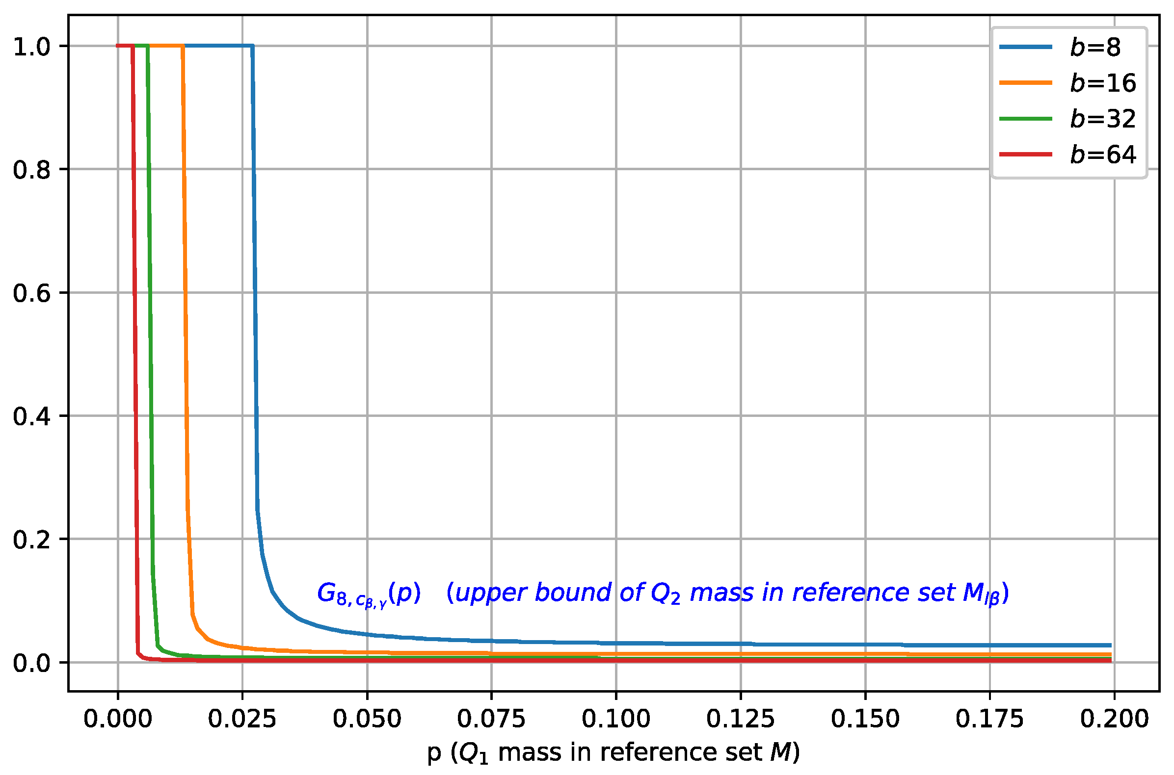
3.2. Probability Mass Separation

In this section, we show that a certain topological constraint on the $(Q_i,Q_j)$ pair will lead to probability mass separation. More precisely, given a reference set $M=B(x_0;r_0)\subseteq \mathcal{Z}$, let $M_{l\cdot \beta }=B(x_0;r_0+l\cdot \beta )$, our topological constraint provides a non-trivial upper bound on $Q_j(M_{l\cdot \beta })$ in terms of $Q_i(M)$.

In order to enforce the separation between two classes, we extend Definition 6 to characterize the separation between two sets:

Definition 7. 

Let$\beta >0$,$\gamma >2\beta$. Considering two sets,$M_1,M_2\subseteq \mathcal{Z}$and$M=M_1\cup M_2$, we denote the death-times of$M$’s 0-dimensional Vietoris-Rips persistent homology as${\left\{d_i\right\}}_{i\in {\mathcal{I}}_0}$and order the indexing of points by decreasing lifetimes, i.e.,$d_i\ge d_j$for$i<j$. Then, we state$M_1$and$M_2$are$(\beta ,\gamma )$-separated, if and only if the following two conditions are satisfied:

(1)$M_1$and$M_2$are both$\beta$-connected;

(2)$d_2$is in the open interval$(\gamma ,\infty )$.

Then we use this notion to capture the concentration and separation of a (b, b) sample from a $(Q_i,Q_j)$ pair. For b-sized i.i.d. samples from $Q$, we denote the product measure of $Q$ by $Q^b$, and for (b, b)-sized samples from $(Q_i,Q_j)$(b i.i.d. draws from each), we denote the product measure by $Q_i^b{Q}_j^b$.

Define the indicator function ${\mathfrak{c}}_{(b,b)}^{\beta ,\gamma }:{\mathcal{Z}}^{(b,b)}\to \{0,1\}$ as follows:

${\mathfrak{c}}_{(b,b)}^{\beta ,\gamma }(z_{1,1},\dots z_{1,b},z_{2,1},\dots z_{2,b})=1\iff \{z_{1,1},\dots z_{1,b}\},\{z_{2,1},\dots z_{2,b}\}$ are $(\beta ,\gamma )$-separated.

Now we consider the probability of the (b, b)-sized samples from $Q_i^b{Q}_j^b$ being $(\beta ,\gamma )$-separated.

Definition 8. 

Let$\beta >0$,$\gamma >2\beta$,$c_{\beta }\in [0,1]$, and$b\in \mathbb{N}$. We call a$(Q_i,Q_j)$pair$(b,c_{\beta ,\gamma })$-separated if:

$$Q_i^b{Q}_j^b(\{{\mathfrak{c}}_{(b,b)}^{\beta ,\gamma }=1\})\ge c_{\beta ,\gamma }$$

(12)

For two classes C₁ and C₂, consider the restriction of $Q$ to C₁ and C₂, i.e., $Q_1$ and $Q_2$. Assume $(Q_1,Q_2)$ is $(b,c_{\beta ,\gamma })$-separated, consider reference set $M=B(x_0;r_0)\subseteq \mathcal{Z}$ and let $M_{l\cdot \beta }=B(x_0;r_0+l\cdot \beta )$, together with the complement set $N=M_{l\cdot \beta }^C$, where $r_0+l\cdot \beta \le \gamma /2$. Let $\mathfrak{p}=Q_1(M)$, $\mathfrak{q}=Q_1(M_{l\cdot \beta })$ and $\mathfrak{s}=Q_2(M_{l\cdot \beta })$. According to [22], when $\mathfrak{p}$ is fixed, we can lower bound $\mathfrak{q}$. In the following, we will provide an approach to upper bound s, which hints at mass separation between different classes.

For a (b, b) sample $(z_{1,1},\dots z_{1,b},z_{2,1},\dots z_{2,b}) ~ Q_1^b{Q}_2^b$, consider the distribution of $z_{i,j}$ among $M_{l\cdot \beta }$ and N. Let $n_1$ and $n_2$ be the numbers of $z_{1,i}$’s and $z_{2,i}$’s that fall within $M_{l\cdot \beta }$, respectively; i.e., $n_1=\left|\left\{z_{1,i}\right\}\cap M_{l\cdot \beta }\right|$ and $n_2=\left|\left\{z_{2,i}\right\}\cap M_{l\cdot \beta }\right|$. Apparently, if the membership assignment satisfies: $n_1\ge 1$ and $n_2\ge 1$, then $(z_{1,1},\dots z_{1,b},z_{2,1},\dots z_{2,b})$ cannot be $(\beta ,\gamma )$-separated.

Thus, we define events that $(z_{1,1},\dots z_{1,b},z_{2,1},\dots z_{2,b})$ cannot be $(\beta ,\gamma )$-separated as follows:

$E=\{(z_{1,1},\dots z_{1,b},z_{2,1},\dots z_{2,b}) ~ Q_1^b{Q}_2^b:n_1\ge 1,n_2\ge 1\}$ and then we have ${\mathfrak{c}}_{(b,b)}^{\beta ,\gamma }(E)=\left\{0\right\}$.

In the following lemma, we compute the probability of event E and derive some useful properties.

Proposition 4. 

Let$b\in \mathbb{N}$,$q,s\in [0,1]$,$\mathfrak{q}=Q_1(M_{l\cdot \beta })$and$\mathfrak{s}=Q_2(M_{l\cdot \beta })$. Denote the following:

$$\mathsf{\Phi }(q,s;b)={\displaystyle \sum _{n_1=1}^b{\displaystyle \sum _{n_2=1}^b\frac{b!}{n_1!(b-n_1)!}\frac{b!}{n_2!(b-n_2)!}}}{q}^{n_1}{(1-q)}^{b-n_1}{s}^{n_2}{(1-s)}^{b-n_2}$$

(13)

Then the probability of E can be expressed in terms of$\mathfrak{q}$and$\mathfrak{s}$as follows:$Q_1^b{Q}_2^b(E)=\mathsf{\Phi }(\mathfrak{q},\mathfrak{s};b)$, and for$\mathsf{\Phi }(q,s;b)$, it holds that

(1)$\mathsf{\Phi }(q_0,\cdot ;b)$is monotonically increasing on$[0,1]$,

(2)$\mathsf{\Phi }(\cdot ,s_0;b)$is monotonically increasing on$[0,1]$.

Proof. 

$$\begin{array}{l}\mathsf{\Phi }(q,s;b)={\displaystyle \sum _{n_1=1}^b{\displaystyle \sum _{n_2=1}^b\frac{b!}{n_1!(b-n_1)!}\frac{b!}{n_2!(b-n_2)!}}}{q}^{n_1}{(1-q)}^{b-n_1}{s}^{n_2}{(1-s)}^{b-n_2}\\ ={\displaystyle \sum _{n_1=1}^b\frac{b!}{n_1!(b-n_1)!}}{q}^{n_1}{(1-q)}^{b-n_1}{\displaystyle \sum _{n_2=1}^b\frac{b!}{n_2!(b-n_2)!}}{s}^{n_2}{(1-s)}^{b-n_2}\end{array}$$

(14)

For argument (1), we fix $q=q_0$ and write

$$\mathsf{\Phi }(q_0,s;b)={\displaystyle \sum _{n_1=1}^b\frac{b!}{n_1!(b-n_1)!}}{q}_0^{n_1}{(1-q_0)}^{b-n_1}\underset{A(s)}{\underbrace{{\displaystyle \sum _{n_2=1}^b\frac{b!}{n_2!(b-n_2)!}}{s}^{n_2}{(1-s)}^{b-n_2}}}$$

(15)

To study the monotonicity properties of $\mathsf{\Phi }(q_0,\cdot ;b)$, it is sufficient to consider $A(s)$.

We define two auxiliary functions:

$$a_{n_2}(s)=\frac{b!}{n_2!(b-n_2)!}{s}^{n_2}{(1-s)}^{b-n_2}$$

(16)

$$c_{n_2}(s)=\frac{b!}{n_2!(b-n_2)!}{s}^{n_2}(b-n_2){(1-s)}^{b-n_2-1}$$

(17)

Then we have $A(s)={\displaystyle \sum _{n_2=1}^b{a}_{n_2}(s)}$, and that

$$c_{n_2}(s)=\left\{\begin{array}{cc}\frac{b!}{n_2!(b - n_2 - 1)!}{s}^{n_2}{(1-s)}^{b-n_2-1},& 0\le n_2<b\\ 0,& n_2=b\end{array}\right.$$

(18)

$$\begin{array}{l}\frac{\partial a_{n_2}(s)}{\partial s}=\frac{b!}{n_2!(b - n_2)!}{n}_2{s}^{n_2-1}{(1-s)}^{b - n_2}-\frac{b!}{n_2!(b - n_2)!}{s}^{n_2}(b-n_2){(1-s)}^{b-n_2-1}\\ =c_{n_2-1}(s)-c_{n_2}(s)\end{array}$$

(19)

Hence,

$$\frac{\partial A(s)}{\partial s}={\displaystyle \sum _{n_2=1}^b{c}_{n_2-1}(s)-c_{n_2}(s)}=c_0(s)-c_b(s)=c_0(s)\ge 0$$

(20)

Consequently, $A(s)$ is monotonically increasing, and thus, so is $\mathsf{\Phi }(q_0,\cdot ;b)$.

For argument (2), the proof is similar and omitted. □

Now we can derive the main theorem:

Theorem 1. 

Let$b\in \mathbb{N}$,$q,s\in [0,1]$,$\mathfrak{q}=Q_1(M_{l\cdot \beta })$and$\mathfrak{s}=Q_2(M_{l\cdot \beta })$. Then it holds that

$$1-c_{\beta ,\gamma }\ge \mathsf{\Phi }(\mathfrak{q},\mathfrak{s};b)$$

(21)

Proof. 

The left side includes all the events that violate the separation assumption, and the right side is only a special case among them. Therefore, by combining Definition 8 and Proposition 4, we complete the proof. □

3.3. Ramifications of Theorem 1

According to Theorem 1 and Proposition 4, if $M_{l\cdot \beta }$ covers a certain mass of $Q_1$, we can upper bound the mass it covers of $Q_2$, i.e., because $\mathsf{\Phi }(\mathfrak{q},\mathfrak{s};b)$ is bounded by $1-c_{\beta ,\gamma }$ and is monotonically increasing in $q$ and $s$, if $\mathfrak{q}=Q_1(M_{l\cdot \beta })$ is greater than some $q_0$, then $\mathfrak{s}=Q_2(M_{l\cdot \beta })$ should be less than some $s_0$. This is beneficial for generalization if $M_{l\cdot \beta }$ is constructed from the representations of the correctly classified training instances to include some minimal mass of C₁.

Assuming that the mass of the reference set $\mathfrak{p}=Q_1(M)$ is fixed, noting that our Definition 7 is stronger than the mass concentration condition in [22] and then letting $\mathsf{\Psi }(p,q;b,l)={\displaystyle \sum _{(u,v,w)\in I(b,l)}\frac{b!}{u!v!w!}{p}^u{(1-q)}^v{(q-p)}^w}$, we have

$$\mathfrak{q}\in \{q\in [\mathfrak{p},1]:1-c_{\beta ,\gamma }\ge \mathsf{\Psi }(\mathfrak{p},\mathfrak{q};b,l)\}=A_1$$

(22)

Let ${\mathcal{R}}_{b,c_{\beta ,\gamma }}(\mathfrak{p},l)=\min A_1$ be the smallest mass in the $l\cdot \beta$ extension, and then $\mathfrak{q}\ge {\mathcal{R}}_{b,c_{\beta ,\gamma }}(\mathfrak{p},l)\ge \mathfrak{p}$.

By Theorem 1, we have

$$\mathfrak{s}\in \left\{s\in [0,1]:1-c_{\beta ,\gamma }\ge \mathsf{\Phi }(\mathfrak{q},\mathfrak{s};b)\ge \mathsf{\Phi }({\mathcal{R}}_{b,c_{\beta ,\gamma }}(\mathfrak{p},l),\mathfrak{s};b)\right\}=A_2$$

(23)

and thus $A_2$ is non-empty. Now let ${\mathcal{T}}_{b,c_{\beta ,\gamma }}(\mathfrak{q})=\max A_2$ identify the largest mass in the $l\cdot \beta$ extension for which the inequality holds. As $\mathfrak{q}$ increases, ${\mathcal{T}}_{b,c_{\beta ,\gamma }}(\mathfrak{q})$ decreases; therefore, $\mathfrak{s}\le {\mathcal{T}}_{b,c_{\beta ,\gamma }}(\mathfrak{q})\le {\mathcal{T}}_{b,c_{\beta ,\gamma }}({\mathcal{R}}_{b,c_{\beta ,\gamma }}(\mathfrak{p},l))$.

Let ${\mathcal{G}}_{b,c_{\beta ,\gamma }}(\mathfrak{p},l)\triangleq {\mathcal{T}}_{b,c_{\beta ,\gamma }}({\mathcal{R}}_{b,c_{\beta ,\gamma }}(\mathfrak{p},l))$, then $\mathfrak{s}\le {\mathcal{G}}_{b,c_{\beta ,\gamma }}(\mathfrak{p},l)$.

As $\mathsf{\Psi }$ is monotonically decreasing in $\mathfrak{q}$, ${\mathcal{R}}_{b,c_{\beta ,\gamma }}(\mathfrak{p})$ is monotonically increasing in $c_{\beta ,\gamma }$; furthermore, as $\mathsf{\Phi }$ is monotonically increasing in s, ${\mathcal{T}}_{b,c_{\beta ,\gamma }}(\mathfrak{q})$ is monotonically decreasing in $c_{\beta ,\gamma }$. These facts motivate our regularization goal of increasing $c_{\beta ,\gamma }$. In other words, increasing $c_{\beta ,\gamma }$ would both boost mass concentration within a class and enforce mass separation between two classes.

Suppose M is constructed mainly by training samples from C₁, i.e., we choose $x_0$ and $r_0$ to include many training samples from C₁; then we can ask the following: how much mass of C₁ should M contain at least to boost the separation?

We plot $\mathsf{\Phi }(\mathfrak{q},\mathfrak{q};b)$ in Figure 1, and we can see that $\mathfrak{q}=\mathfrak{s}$ at point (0.049, 0.049), i.e., $\mathsf{\Phi }(\mathfrak{q},\mathfrak{q};b)=1-c_{\beta ,\gamma }$. At this point, the mass separation effect starts to occur. To satisfy Inequality (21), when $\mathfrak{q}$ increases, $\mathfrak{s}$ should decrease, which means that as $M_{l\cdot \beta }$ covers more mass of $Q_1$, it covers less mass of $Q_2$. In addition, as the batch size b increases, the least mass of $Q_1$ that $M_{l\cdot \beta }$ should cover decreases.

In Figure 2, we fix the batch size to 8 and visualize $\mathsf{\Phi }(\mathfrak{q},\mathfrak{s};b)$ as a function of $\mathfrak{s}$ (for different values of $\mathfrak{q}$), and we can see that when $\mathfrak{q}$ increases, ${\mathcal{T}}_{b,c_{\beta ,\gamma }}(\mathfrak{q})$ moves towards zero, which indicates a smaller $\mathfrak{s}$, i.e., $M_{l\cdot \beta }$ covers less mass of $Q_2$, and therefore, it leads to a better separation.

In Figure 3, we plot ${\mathcal{T}}_{b,c_{\beta ,\gamma }}(\mathfrak{q})$ as a function of $\mathfrak{q}$ for different values of $c_{\beta ,\gamma }$, where $\mathfrak{q}=Q_1(M_{l\cdot \beta })$. As $c_{\beta ,\gamma }$ is increased, the maximal mass of $Q_2$ contained in $M_{l\cdot \beta }$, characterized by ${\mathcal{T}}_{b,c_{\beta ,\gamma }}(\mathfrak{q})$, shifts towards a smaller value, which indicates that a better separation between classes C₁ and C₂ is achieved.

Figure 4 visualizes ${\mathcal{G}}_{b,c_{\beta ,\gamma }}(\mathfrak{p},l)$ as a function of $\mathfrak{p}$ for different values of $c_{\beta ,\gamma }$, where $\mathfrak{p}=Q_1(M)$. It can be seen that as $c_{\beta ,\gamma }$ is increased, the maximal mass of $Q_2$ contained in $M_{l\cdot \beta }$, characterized by ${\mathcal{G}}_{b,c_{\beta ,\gamma }}(\mathfrak{p},l)$, also shifts towards a smaller value, which indicates a better separation.

Figure 5 plots ${\mathcal{G}}_{b,c_{\beta ,\gamma }}(\mathfrak{p},l)$ as a function of $\mathfrak{p}$ for different values of batch size b, where $\mathfrak{p}=Q_1(M)$. As b is increased, the maximal mass of $Q_2$ contained in $M_{l\cdot \beta }$, characterized by ${\mathcal{G}}_{b,c_{\beta ,\gamma }}(\mathfrak{p},l)$, also shifts towards a smaller value, which indicates a better separation, and in order to achieve separation, M only needs to cover a small mass of $Q_1$.

3.4. Weighted Rips Filtration and Regularization

In Section 3.2, we show that a topological constraint on a $(Q_i,Q_j)$ pair would lead to probability mass concentration and separation. To impose this constraint, we propose a function that is used to construct the filtration, and then we compute the 0-dimensional persistent diagram and construct the loss item to regularize the internal representation.

Our method acts on the level of mini-batches; we construct each mini-batch B as a collection of n sub-batches, i.e., B = (B₁,…, B_n), as in [22]. Each sub-batch consists of b samples from the same class, and thus the resulting mini-batch B contains n*b samples. Our regularizer consists of three items and penalizes deviations from a $(\beta ,\gamma )$-separated arrangement of $(z_{1,1},\dots z_{1,b},z_{2,1},\dots z_{2,b})$ for all sub-batch pairs (B_i, B_j).

3.4.1. A Weight Function for Weighted Rips Filtration

To construct a proper filtration to deal with samples from two different classes, we define a function $f$:

$$f_{\mu ,\nu ,m,T}(x)=\ln (1+\exp ((d_{\mu ,m}(x)-d_{\nu ,m}(x))/T))$$

(24)

where T is the temperature that controls the magnitude and $d_{\mu ,m}(x)$ is the DTM function defined in Equation (7).

Considering the mass separation for two classes, we denote the data instances of class $k$ by $S_k$, and then for a class pair $(C_i,C_j)$, the training samples can be written as follows: $S_{i,j}=S_i\cup S_j$. Let $Q_i$ and $Q_j$ be the restriction of $Q$ (i.e., the push-forward of $P$ via $\phi$) to classes i and j, respectively. In order to construct filtration with Equation (24), firstly, we need to compute $f_{Q_i,Q_j,m,T}(x)$ for $x\in S_{i,j}$. Note that $d_{Q_i,m}$ and $d_{Q_j,m}$ can be computed with Equation (9), the DTEM, where $Q_i$ is approximated by $\phi (S_i)$ and $Q_j$ is approximated by $\phi (S_j)$. According to Equation (24), for a good classifier, points from class i should have smaller function values than points from class j. Then we plug $f_{Q_i,Q_j,m,T}(x)$ into Equation (4) to compute the weighted Rips filtration (we set p = 1 for Equation (4) in this research), and obtain the 0-dimensional persistence diagram, i.e., the multi-set of intervals for homology in dimension 0, $\mathrm{P}{\mathrm{D}}_0({\mathcal{X}}_{i,j})={\{(b_k,d_k)\}}_{k\in I_0}$. After that, we order the indexing of points by decreasing lifetimes as done in Definition 7; we will use them later to construct the loss item in Section 3.4.3.

3.4.2. Stability

In this section, we establish the stability results for our weight function in Equation (24). In Theorem 2, the stability of the weight function is given, which will later be used in Theorem 3 to ensure the stability of the filtration $V[X,f]$ with respect to the weight function $f$. Proposition 5 is used to ensure the stability of the filtration $V[X,f]$ with respect to $X$. According to persistent homology theory, the stability results for the filtration translate as stability results for the persistence diagrams. We present our main stability results in Theorem 3.

Theorem 2. 

Let${\mu }_1$,${\mu }_2$,${\nu }_1$ and ${\nu }_2$ be four probability measures, and $m\in (0,1)$. Then

$${‖f_{{\mu }_1,{\mu }_2,m,T}-f_{{\nu }_1,{\nu }_2,m,T}‖}_{\infty }\le (1/T)m^{-(1/2)}(W_2({\mu }_1,{\nu }_1)+W_2({\mu }_2,{\nu }_2))$$

(25)

Proof. 

Let $h_{{\mu }_1,{\mu }_2,m,T}(x)=(d_{{\mu }_1,m}(x)-d_{{\mu }_2,m}(x))/T$ and $g(x)=\ln (1+\exp (x))$. Then $f=g\circ h$.

Because $g(x)$ is 1-Lipschitz, i.e., for all $x$ and $y$, $\left|g(x)-g(y)\right|\le \left|x-y\right|$, we have

$$\begin{array}{l}{‖f_{{\mu }_1,{\mu }_2,m,T}-f_{{\nu }_1,{\nu }_2,m,T}‖}_{\infty }={‖g\circ h_{{\mu }_1,{\mu }_2,m,T}-g\circ h_{{\nu }_1,{\nu }_2,m,T}‖}_{\infty }\le {‖h_{{\mu }_1,{\mu }_2,m,T}-h_{{\nu }_1,{\nu }_2,m,T}‖}_{\infty }=\\ (1/T){‖(d_{{\mu }_1,m}-d_{{\mu }_2,m})-(d_{{\nu }_1,m}-d_{{\nu }_2,m})‖}_{\infty }\le (1/T)({‖d_{{\mu }_1,m}-d_{{\nu }_1,m}‖}_{\infty }+{‖d_{{\mu }_2,m}-d_{{\nu }_2,m}‖}_{\infty })\\ \le (1/T)m^{-(1/2)}(W_2({\mu }_1,{\nu }_1)+W_2({\mu }_2,{\nu }_2))\end{array}$$

(26)

The last inequality is obtained according to Proposition 2. □

In Proposition 5, we consider the stability of the filtration with respect to $X$. For brevity, the subscripts of $f$ are omitted.

Proposition 5. 

Suppose that$X$and$Y$are compact and that the Hausdorff distance$d_H(X,Y)\le \epsilon$. Then the filtrations$V[X,f]$and$V[Y,f]$are k-interleaved with$k=\epsilon (1+2/T)$.

Proof. 

It suffices to show that for every $t\ge 0$, $V_t[X,f]\subseteq V_t[Y,f]$.

For $z\in V_t[X,f]$, there exists $x\in X$ such that $z\in {\overline{B}}_f(x,t)$, i.e., $‖x-z‖\le r_x(t)$. From the hypothesis $d_H(X,Y)\le \epsilon$, there exists $y\in Y$ such that $‖x-y‖\le \epsilon$. Then we need to prove that $z\in {\overline{B}}_f(y,t+k)$, i.e., $‖z-y‖\le r_y(t+k)$.

According to triangle inequality, $‖z-y‖\le ‖z-x‖+‖x-y‖\le r_x(t)+\epsilon$. Then it suffices to show that $r_x(t)+\epsilon \le r_y(t+k)$.

Using Equation (4), we have

$$\begin{array}{l}{r}_y(t+k)-r_x(t)=((t+k)-f(y))-(t-f(x))=k+(f(x)-f(y))\\ =k+(g(h(x))-g(h(y)))\ge k-\left|h(x)-h(y)\right|\\ =k-(1/T)\left(\left|(d_{{\mu }_1,m}(x)-d_{{\mu }_2,m}(x))-(d_{{\mu }_1,m}(y)-d_{{\mu }_2,m}(y))\right|\right)\end{array}$$

(27)

According to Proposition 1, the DTM function is 1-Lipschitz, and then

$$\begin{array}{l}\left|(d_{{\mu }_1,m}(x)-d_{{\mu }_2,m}(x))-(d_{{\mu }_1,m}(y)-d_{{\mu }_2,m}(y))\right|\le \left|d_{{\mu }_1,m}(x)-d_{{\mu }_1,m}(y)\right|+\left|d_{{\mu }_2,m}(x)-d_{{\mu }_2,m}(y)\right|\\ \le 2‖x-y‖\le 2\epsilon \end{array}$$

(28)

Therefore,

$$r_y(t+k)-r_x(t)\ge k-(2/T)\epsilon =\epsilon (1+2/T)-(2/T)\epsilon =\epsilon . \square$$

In the following theorem, we combine the above results to establish the stability of the persistence diagram with respect to $X$ and $f$.

Theorem 3. 

Consider four measures${\mu }_1$,${\mu }_2$,${\nu }_1$and${\nu }_2$on${ℝ}^d$with compact supports$X_1$,$X_2$,$Y_1$and$Y_2$, respectively. Let$X=X_1\cup X_2$,$Y=Y_1\cup Y_2$,$V_1=V[X,f_{{\mu }_1,{\mu }_2,m,T}]$and$V_2=V[Y,f_{{\nu }_1,{\nu }_2,m,T}]$,$d_b$denotes the bottleneck distance between persistence diagrams. Then

$$d_b(D(V_1),D(V_2))\le (1/T)m^{-(1/2)}(W_2({\mu }_1,{\nu }_1)+W_2({\mu }_2,{\nu }_2))+(1+2/T)d_H(X,Y)$$

(29)

Proof. 

Under some regularity conditions, $d_b(D(V_1),D(V_2))=d_i(V_1,V_2)$, where $d_i$ denotes the interleaving pseudo-distance between two filtrations as defined in Equation (3).

We use the triangle inequality for the interleaving distance:

$$d_i(V_1,V_2)\le \underset{(1)}{\underbrace{d_i(V[X,f_{{\mu }_1,{\mu }_2,m,T}],V[Y,f_{{\mu }_1,{\mu }_2,m,T}])}}+\underset{(2)}{\underbrace{d_i(V[Y,f_{{\mu }_1,{\mu }_2,m,T}],V[Y,f_{{\nu }_1,{\nu }_2,m,T}])}}$$

(30)

For the first part (1) on the right side of Equation (30), it can be seen that from Proposition 5, we have

$$d_i(V[X,f_{{\mu }_1,{\mu }_2,m,T}],V[Y,f_{{\mu }_1,{\mu }_2,m,T}])\le (1+2/T)d_H(X,Y)$$

For the second part (2) on the right side of Equation (30), according to Proposition 3.2 in [25], we have

$$d_i(V[Y,f_{{\mu }_1,{\mu }_2,m,T}],V[Y,f_{{\nu }_1,{\nu }_2,m,T}])\le {‖f_{{\mu }_1,{\mu }_2,m,T}-f_{{\nu }_1,{\nu }_2,m,T}‖}_{\infty }$$

(31)

Using Theorem 2, we have

$${‖f_{{\mu }_1,{\mu }_2,m,T}-f_{{\nu }_1,{\nu }_2,m,T}‖}_{\infty }\le (1/T)m^{-(1/2)}(W_2({\mu }_1,{\nu }_1)+W_2({\mu }_2,{\nu }_2))$$

By combining part (1) and part (2), we complete the proof. □

3.4.3. Regularization via Persistent Homology

We split the persistence intervals obtained in Section 3.4.1 into two subsets:

$$\mathrm{P}{\mathrm{D}}_0({\mathcal{X}}_{i,j})={\{(b_k,d_k)\}}_{k\in I_0}={\{(b_{i,k},d_{i,k})\}}_{k\in I_{0,i}}\cup {\{(b_{j,k},d_{j,k})\}}_{k\in I_{0,j}}$$

where ${\{(b_{i,k},d_{i,k})\}}_{k\in I_{0,i}}$ consists of the intervals in which the birth time belongs to class i and ${\{(b_{j,k},d_{j,k})\}}_{k\in I_{0,j}}$ consists of the intervals in which the birth time belongs to class j.

Now we define three loss items:

• Birth loss

Birth loss is designed to measure intra-class distance, in order to meet the first requirement of Definition 6, to enforce intra-class mass concentration:

$${\mathcal{L}}_{\mathrm{birth}}(B_i,B_j)={\displaystyle \sum _{k\in I_{0,i}}\left|b_{i,k}-b_0\right|}+{\displaystyle \sum _{k\in I_{0,j}}\left|b_{j,k}-b_1\right|}$$

(32)

where $b_0$ and $b_1$ are super parameters used to control the birth time for each class.

• Margin loss

Margin loss is designed to measure the “distance” between two classes. There may be connected components that appear due to points from class i but disappear due to points from class j, these cases should be penalized. In addition, for class j, the longest interval in ${\{(b_{j,k},d_{j,k})\}}_{k\in I_{0,j}}$ would finally merge into class i’s intervals.

Let $b_{j,\min }=\min \{b_{j,k}:k\in I_{0,j}\}$; we define

$${\mathcal{L}}_{\mathrm{margin}}(B_i,B_j)={\displaystyle \sum _{k\in I_{0,i}}\max \left(\gamma +(d_{i,k}-b_{j,\min }),0\right)}$$

(33)

which means that we penalize the margins $b_{j,\min }-d_{i,k}$ smaller than $\gamma$, where $\gamma$ is also a super parameter used to control inter-class separation.

• Length loss

Weighted Rips filtration is not as direct as the Rips filtration in controlling distances. Therefore, the length loss can be used in combination with the birth loss to penalize large intra-class distances. In addition, we hope that the two classes correspond to two connected components, which will persist for a wide range of parameters until these two components finally merge when the parameter reaches a sufficiently large value. We also want to prevent $Q_k$ from becoming overly dense. To formulate this intuition, we define

$${\mathcal{L}}_{\mathrm{length}}(B_i,B_j)={\displaystyle \sum _{k\in I_{0,i}}\left|d_{i,k}-b_{i,k}-\beta \right|}+{\displaystyle \sum _{k\in I_{0,j}}\left|d_{j,k}-b_{j,k}-\beta \right|}$$

(34)

where $\beta$ is a super parameter.

Finally, our regularization item can be written as follows:

$$\mathcal{L}(B_i,B_j)={\lambda }_1{\mathcal{L}}_{\mathrm{birth}}(B_i,B_j)+{\lambda }_2{\mathcal{L}}_{\mathrm{margin}}(B_i,B_j)+{\lambda }_3{\mathcal{L}}_{\mathrm{length}}(B_i,B_j)$$

(35)

where the weightings ${\lambda }_1$, ${\lambda }_2$ and ${\lambda }_3$ can be set such that the range of the loss is comparable, in range, to the cross-entropy loss, or can be selected via cross-validation.

4. Experiments

In this section, we test our idea with some experiments. We first consider point cloud optimization to obtain some intuition on the behavior of (35), and then we evaluate our approach on the image classification task.

4.1. Point Cloud Optimization

To validate our approach, as an illustrative example, we perform point cloud optimization with only the proposed loss in Equation (35), without other loss items. Point clouds are generated from Gaussian mixture distribution, and we assume that these points are from two different classes: C₁ and C₂. In the following figures, purple points represent samples from C₁, and red points represent samples from C₂.

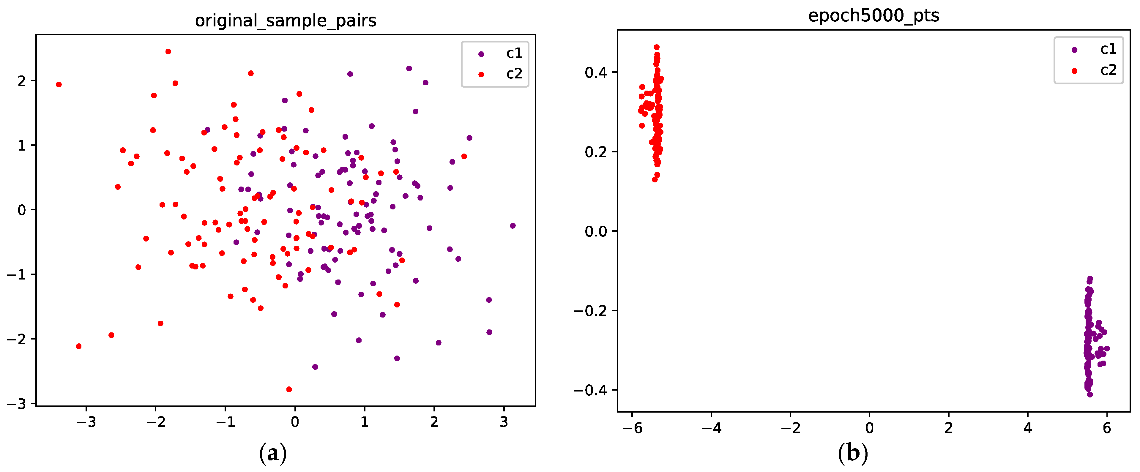
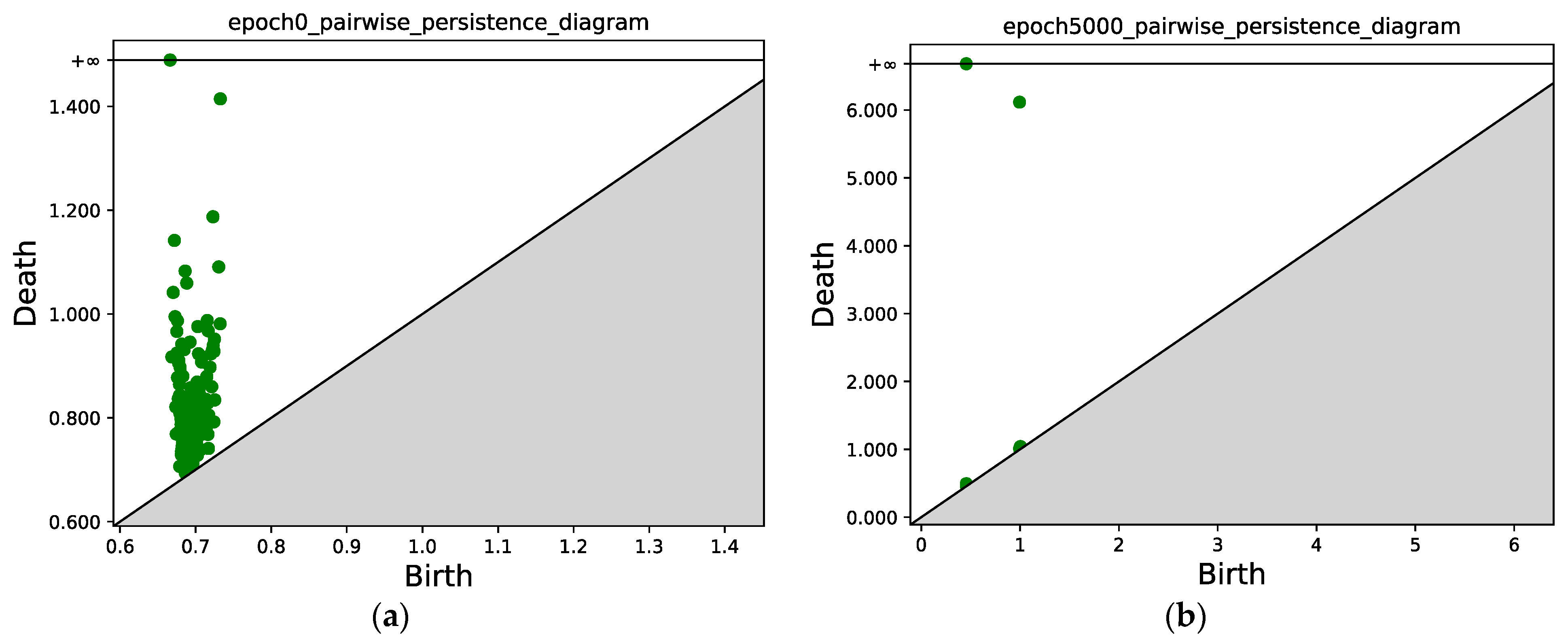
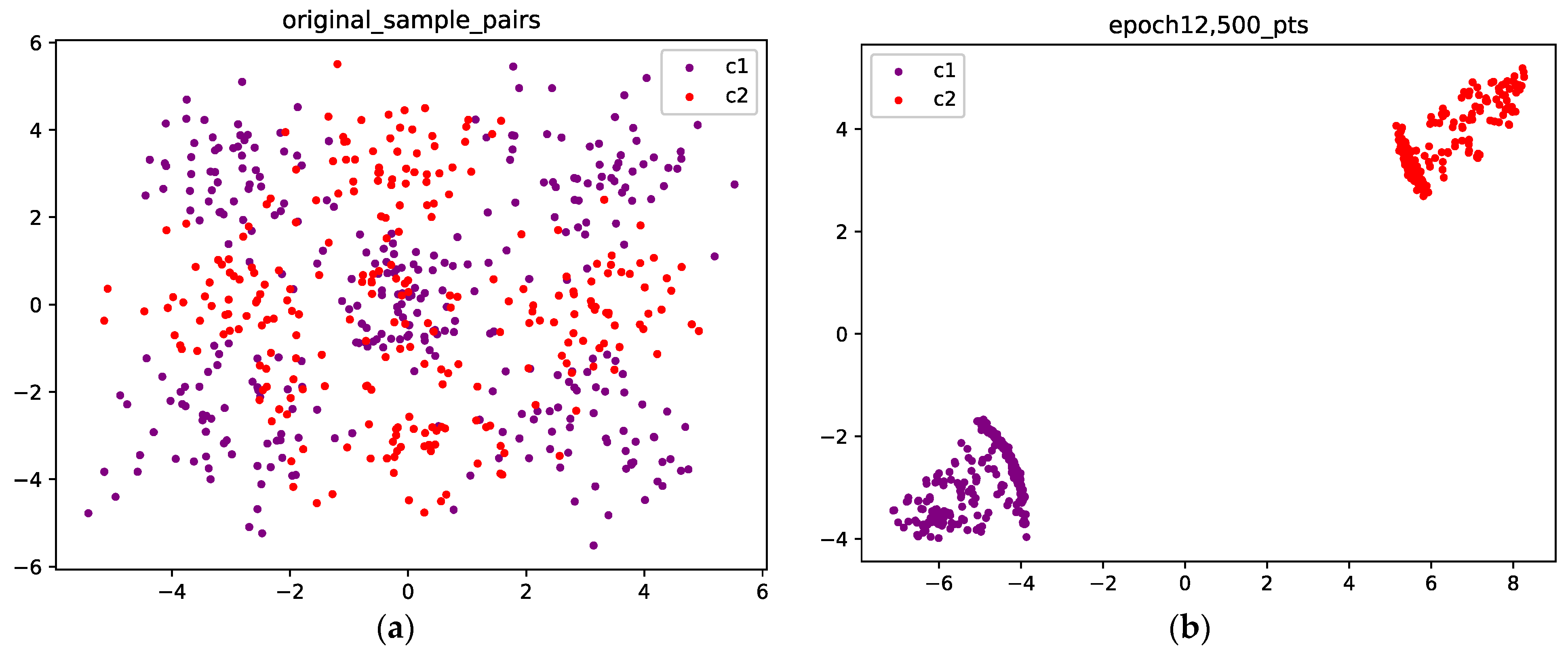
4.1.1. Gaussian Mixture with Two Components

To test the separation effect, we set the centers of the two components to (−0.6, 0) and (0.6, 0), and the covariance matrix is set to the identity matrix. For parameters in the weight function of Equation (24), we set $m=0.1$ and $1/T=0.05$. For super parameters in the three loss items, we set $b_0=0$, $b_1=1.0$, $\beta =0$ and $\gamma =0.6$. To encourage clustering and speed up optimization, we adopt a dynamic m update scheme, i.e., gradually increasing m during training. The weightings of the three loss functions are set to 9, 1 and 0.3, respectively, and are chosen by gradient information in the first epoch.

Figure 6a shows the initial position of the points; the purple points are sampled from C₁, and the red points are sampled from C₂. Figure 6b shows the final position after 5000 epochs; the mass concentration and separation effects are obvious, and the points from the two classes are well separated.

Since the weight function $f(x)$ may lead to imbalanced point configurations for the two classes, we can address this issue by changing the order of the two sets of points alternatively when feeding data to the computation of persistent homology during training. For vision datasets, because our regularization is used together with cross-entropy loss and a stochastic mini-batch sampling scheme, the imbalance will be compensated automatically.

Figure 7 compares the persistence diagrams before and after training; each green point represents a (b_i, d_i) pair, the green point with y = inf represents the final merged single component left when the filtration value is sufficiently large, and the green point with y > 6 tells us that at this value, the two components merge, i.e., one component disappears and merges into the other component which is generated at an earlier time. In Figure 7, we can see that after 5000 epochs, the two subsets mentioned in Section 3.4.3 that correspond to the two classes are well separated, i.e., two connected components can be identified in the persistence diagram. We can also see that the points from the same class are concentrated.

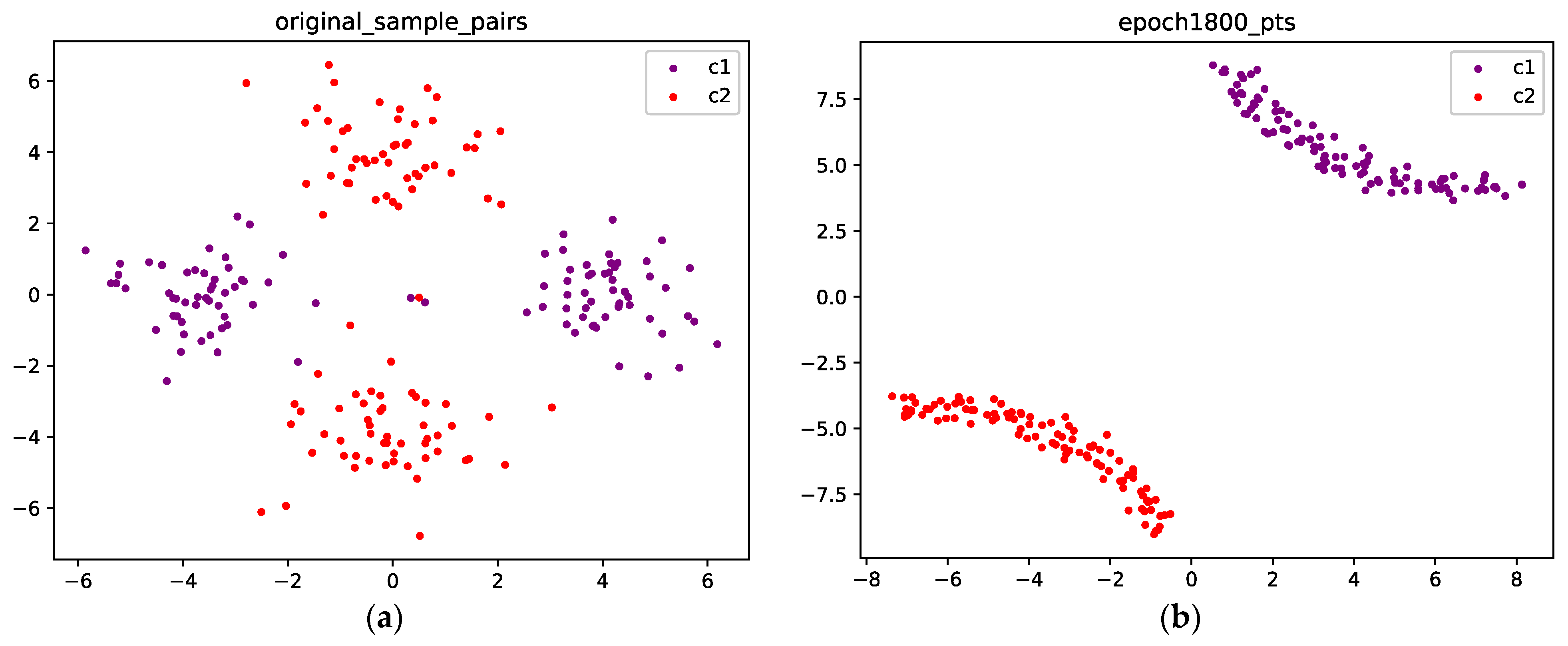
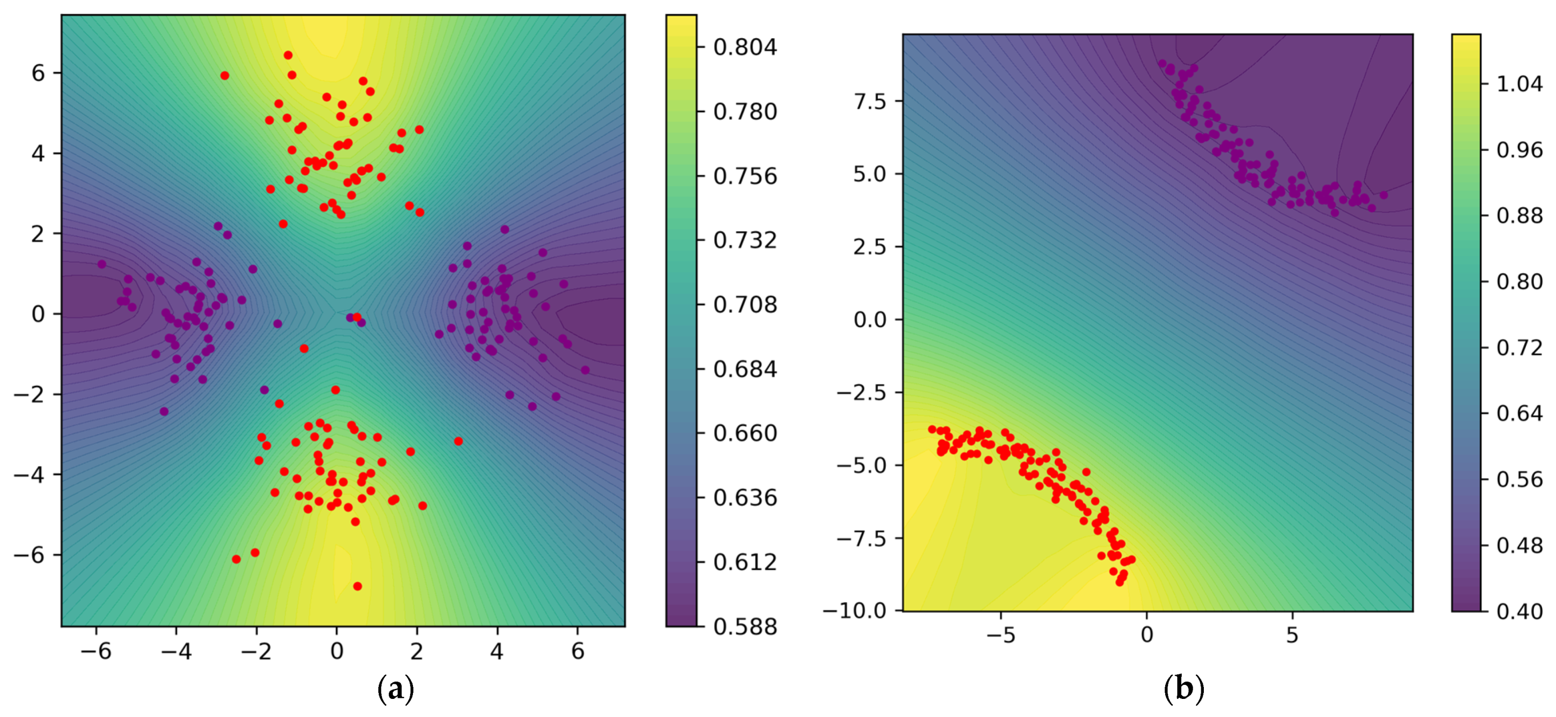
4.1.2. Gaussian Mixture with Four Components

As a more challenging example, we consider a Gaussian mixture with four components. We suppose that they represent samples from two different classes, i.e., each class corresponds to two components. For each class, we hope the corresponding two components can merge. To achieve this goal, samples from one class have to travel across samples from the other class, which may cause the loss to increase. Therefore, to obtain optimal results, the optimizer needs to climb the mountain in the loss landscape before it arrives at a valley.

Figure 8 visualizes the points before and after training. Figure 8a shows the initial position of the points. The purple points are sampled from C₁, and the red points are sampled from C₂. We can see that after 1800 epochs, for each class, the two components merge into a single connected component, as shown in Figure 8b.

Figure 9 visualizes the function values calculated by our weight function (24); these values are used to construct the weighted Rips filtration using Equation (4) to extract topological information, and finally, the topological information is used by the regularizer to guide the optimization. Figure 9a visualizes the function values and the contour lines at epoch 0; it can be seen that larger values are assigned for points from C₂. Figure 9b visualizes the function values and the contour lines after 1800 epochs.

Similar to Figure 7, Figure 10 compares the persistence diagrams before and after training. Figure 10b shows that after 1800 epochs, two connected components can be identified, and the mass concentration and separation effect is obvious.

4.1.3. Gaussian Mixture with Nine Components

In Figure 11 and Figure 12, we present the results for a Gaussian mixture with nine components. Figure 11a shows the initial position of the points sampled from two classes, while Figure 11b shows the results after 12,500 epochs. Figure 12 compares the persistence diagrams before and after training; it can be seen that our method achieves an effective performance in separating samples from two different classes.

4.2. Datasets

In this part, we use the same models and settings as [22], and we evaluate our method on three vision benchmark datasets: MNIST [26], SVHN [27] and CIFAR10 [28]. For MNIST and SVHN, 250 instances are used for training the model, for CIFAR10, 500 and 1000 instances are used.

CNN-13 [29] architecture is employed for CIFAR10 and SVHN. For MNIST, a simpler CNN architecture is employed. We use a stochastic gradient descent (SGD) optimizer with a momentum of 0.9, and the cosine annealing learning rate scheduler [30] is employed.

With the cross-entropy loss, the weighting of our regularization term is set such that the loss in Equation (35) is comparable to the cross-entropy loss. In our experiments, each batch contains n = 8 sub-batches, and the sub-batch size is set to b = 16; thus, the total batch size is 128.

During training, for each epoch, we select the 10 most significant channels dynamically for each class to perform topological computation; the criterion for channel selection is similar to that in [31]. To compensate for the imbalance between two classes induced by the weight function, we use the ratio of the derivative to weight the two items in the birth loss (Equation (32)). In order to meet the stability requirements of topological computation, we use 0.001 as the minimal differentiable distance between points. The weighting of our regularization term is set to 0.001. For parameters in the weight function (24), we set $m=0.2$ and $1/T=0.15$. For super parameters in the three loss items, we set $b_0=0.1$, $b_1=2.5$, $\beta =0.3$, and $\gamma =1.8$; weight decay on $\phi$ is fixed to 1 × 10⁻³, and weight decay on $\eta$ is fixed to 0.001, except for CIFAR10-1k, for which we set it to 5 × 10⁻⁴. On MNIST, the initial learning rate is fixed to 0.1. On SVHN and CIFAR10, it is fixed to 0.5.

Table 1. Comparison to previous regularizers. “Vanilla” includes batch normalization, dropout and weight decay. The average test error and the standard deviation are reported.

Regularization	MNIST-250	SVHN-250	CIFAR10-500	CIFAR10-1k
Vanilla	7.1 ± 1.0	30.1 ± 2.9	39.4 ± 1.5	29.5 ± 0.8
+Jac.-Reg [9]	6.2 ± 0.8	33.1 ± 2.8	39.7 ± 2.0	29.8 ± 1.2
+DeCov [1]	6.5 ± 1.1	28.9 ± 2.2	38.2 ± 1.5	29.0 ± 0.6
+VR [2]	6.1 ± 0.5	28.2 ± 2.4	38.6 ± 1.4	29.3 ± 0.7
+cw-CR [2]	7.0 ± 0.6	28.8 ± 2.9	39.0 ± 1.9	29.1 ± 0.7
+cw-VR [2]	6.2 ± 0.8	28.4 ± 2.5	38.5 ± 1.6	29.0 ± 0.7
+Sub-batches	7.1 ± 0.5	27.5 ± 2.6	38.3 ± 3.0	28.9 ± 0.4
+Sub-batches + Top.-Reg [22]	5.6 ± 0.7	22.5 ± 2.0	36.5 ± 1.2	28.5 ± 0.6
+Sub-batches + Top.-Reg [22]	5.9 ± 0.3	23.3 ± 1.1	36.8 ± 0.3	28.8 ± 0.3
+Sub-batches + Top.-Reg(Ours)	4.3 ± 0.3	22.9 ± 1.3	35.2 ± 0.6	27.4 ± 0.6

compares our method to Vanilla (including batch normalization, dropout and weight decay) and the regularizers proposed in relevant works, in particular, the regularizers based on statistics of representations [1,2] and the topological regularizer as proposed in [22]. In addition, we also provide results given by the Jacobian regularizer [9]. We report the average test error (%) and the standard deviation over 10 cross-validation runs. The number attached to the dataset names indicates the number of training instances used. It can be seen that our method achieves the lowest average error for MNIST-250, CIFAR10-500, and CIFAR10-1k. For SVHN, the mean error is a little higher than the result presented in [22], but our method achieves a lower variance. Especially, our method outperforms all the regularization methods based on statistical constraints by a significant margin, which demonstrates the advantage of the proposed topology-aware regularizer, and this also supports our claim that mass separation is beneficial.

5. Conclusions

Traditionally, statistical methods are employed to impose constraints on the internal representation space for deep neural networks, while topological methods are generally underexploited. In this paper, we took a fundamentally different perspective to control internal representation with tools from TDA. By utilizing persistent homology, we constrained the push-forward probability measure and enhanced mass separation in the internal representation space. Specifically, we formulated a property of this measure that is beneficial for generalization for the first time, and we proved that a topological constraint in the representation space leads to mass separation. Moreover, we proposed a novel weight function for weighted Rips filtration, proved its stability and introduced a regularizer that operates on the persistence diagram obtained via persistent homology to control the distribution of the internal representations.

We evaluated our approach in the point cloud optimization task and the image classification task. For the point cloud optimization task, experiments showed that our method can separate points from different classes effectively. For the image classification task, experiments showed that our method significantly outperformed the previous relevant regularization methods, especially those methods based on statistical constraints.

In summary, both theoretical analysis and experimental results showed that our method can provide an effective learning signal utilizing topological information to guide internal representation learning. Our work demonstrated that persistent homology may serve as a novel and powerful tool for promoting topological structure in the internal representation space. Areas for future research are the exploration of the potential of 1-dimensional persistent homology and the development of other topology-aware methods for deep neural networks.

References

1. Cogswell, M.; Ahmed, F.; Girshick, R.; Zitnick, L.; Batra, D. Reducing Overfitting in Deep Networks by Decorrelating Representations. In Proceedings of the International Conference on Learning Representations, San Juan, PR, USA, 2–4 May 2016. [Google Scholar]
2. Choi, D.; Rhee, W. Utilizing Class Information for Deep Network Representation Shaping. In Proceedings of the AAAI Conference on Artificial Intelligence, Honolulu, HI, USA, 27 January 2019. [Google Scholar]
3. Moor, M.; Horn, M.; Rieck, B.; Borgwardt, K. Topological Autoencoders. In Proceedings of the 37th International Conference on Machine Learning, Online, 13–18 July 2020. [Google Scholar]
4. Raghu, M.; Gilmer, J.; Yosinski, J.; Sohl-Dickstein, J. SVCCA: Singular Vector Canonical Correlation Analysis for Deep Learning Dynamics and Interpretability. In Proceedings of the Advances in Neural Information Processing Systems, Long Beach, CA, USA, 4–9 December 2017. [Google Scholar]
5. Littwin, E.; Wolf, L. Regularizing by the variance of the activations’ sample-variances. In Proceedings of the Advances in Neural Information Processing Systems, Montreal, QC, Canada, 2–8 December 2018. [Google Scholar]
6. Pang, T.Y.; Xu, K.; Dong, Y.P.; Du, C.; Chen, N.; Zhu, J. Rethinking Softmax Cross-Entropy Loss for Adversarial Robustness. In Proceedings of the International Conference on Learning Representations, Addis Ababa, Ethiopia, 26 April 2020. [Google Scholar]
7. Zhu, W.; Qiu, Q.; Huang, J.; Calderbank, R.; Sapiro, G.; Daubechies, I. LDMNet: Low Dimensional Manifold Regularized Neural Networks. In Proceedings of the IEEE Conference on Computer Vision and Pattern Recognition, Salt Lake City, UT, USA, 18–23 June 2018. [Google Scholar]
8. Carlsson, G. Topology and Data. Bull. Am. Math. Soc. 2009, 46, 255–308. [Google Scholar] [CrossRef] [Green Version]
9. Hoffman, J.; Roberts, D.; Yaida, S. Robust Learning with Jacobian Regularization. arXiv 2019, arXiv:1908.02729. [Google Scholar]
10. Kingma, D.P.; Welling, M. Auto-Encoding Variational Bayes. In Proceedings of the International Conference on Learning Representations, Banff, AB, Canada, 14–16 April 2014. [Google Scholar]
11. Chazal, F.; Michel, B. An Introduction to Topological Data Analysis: Fundamental and Practical Aspects for Data Scientists. Front. Artif. Intell. 2017, 4, 667963. [Google Scholar] [CrossRef] [PubMed]
12. Herbert, E.; John, H. Computational Topology: An Introduction; American Mathematical Society: Providence, RI, USA, 2010. [Google Scholar]
13. Hensel, F.; Moor, M.; Rieck, B. A Survey of Topological Machine Learning Methods. Front. Artif. Intell. 2021, 4, 681108. [Google Scholar] [CrossRef]
14. Brüel-Gabrielsson, R.; Nelson, B.J.; Dwaraknath, A.; Skraba, P.; Guibas, L.J.; Carlsson, G. A topology layer for machine learning. In Proceedings of the International Conference on Artificial Intelligence and Statistics, Online, 26–28 August 2020. [Google Scholar]
15. Kim, K.; Kim, J.; Zaheer, M.; Kim, J.S.; Chazal, F.; Wasserman, L. PLLay: Efficient Topological Layer Based on Persistence Landscapes. In Proceedings of the Advances in Neural Information Processing Systems, Online, 6–12 December 2020. [Google Scholar]
16. Hajij, M.; Istvan, K. Topological Deep Learning: Classification Neural Networks. arXiv 2021, arXiv:2102.08354. [Google Scholar]
17. Li, W.; Dasarathy, G.; Ramamurthy, K.N.; Berisha, V. Finding the Homology of Decision Boundaries with Active Learning. In Proceedings of the Advances in Neural Information Processing Systems, Online, 6–12 December 2020. [Google Scholar]
18. Chen, C.; Ni, X.; Bai, Q.; Wang, Y. A Topological Regularizer for Classifiers via Persistent Homology. In Proceedings of the International Conference on Artificial Intelligence and Statistics, Naha, Japan, 16–18 April 2019. [Google Scholar]
19. Vandaele, R.; Kang, B.; Lijffijt, J.; De Bie, T.; Saeys, Y. Topologically Regularized Data Embeddings. In Proceedings of the International Conference on Learning Representations, Online, 25–29 April 2022. [Google Scholar]
20. Hofer, C.; Kwitt, R.; Dixit, M.; Niethammer, M. Connectivity-Optimized Representation Learning via Persistent Homology. In Proceedings of the 36th International Conference on Machine Learning, Long Beach, CA, USA, 9–15 June 2019. [Google Scholar]
21. Wu, P.; Zheng, S.; Goswami, M.; Metaxas, D.; Chen, C. A Topological Filter for Learning with Label Noise. In Proceedings of the Advances in Neural Information Processing Systems, Online, 6–12 December 2020. [Google Scholar]
22. Hofer, C.D.; Graf, F.; Niethammer, M.; Kwitt, R. Topologically Densified Distributions. In Proceedings of the 37th International Conference on Machine Learning, Online, 13–18 July 2020. [Google Scholar]
23. Sizemore, A.E.; Phillips-Cremins, J.; Ghrist, R.; Bassett, D.S. The Importance of the Whole: Topological Data Analysis for the Network Neuroscientist. Netw. Neurosci. 2019, 3, 656–673. [Google Scholar] [CrossRef] [PubMed]
24. Chazal, F.; Cohen-Steiner, D.; Merigot, Q. Geometric Inference for Probability Measures. Found. Comput. Math. 2011, 11, 733–751. [Google Scholar] [CrossRef]
25. Anai, H.; Chazal, F.; Glisse, M.; Ike, Y.; Inakoshi, H.; Tinarrage, R.; Umeda, Y. DTM-Based Filtrations. In Proceedings of the 35th International Symposium on Computational Geometry, Portland, OR, USA, 18–21 June 2019. [Google Scholar]
26. LeCun, Y.; Bottou, L.; Bengio, Y.; Haffner, P. Gradient-based learning applied to document recognition. Proc. IEEE 1998, 86, 2278–2324. [Google Scholar] [CrossRef] [Green Version]
27. Netzer, Y.; Wang, T.; Coates, A.; Bissacco, A.; Wu, B.; Ng, A.Y. Reading Digits in Natural Images with Unsupervised Feature Learning. In Proceedings of the Conference on Neural Information Processing Systems, Granada, Spain, 12–17 December 2011. [Google Scholar]
28. Krizhevsky, A. Learning Multiple Layers of Features from Tiny Images; Technical Report; University of Toronto: Toronto, ON, Canada, 2009. [Google Scholar]
29. Laine, S.; Aila, T. Temporal ensembling for semisupervised learning. In Proceedings of the International Conference on Learning Representations, Toulon, France, 24–26 April 2017. [Google Scholar]
30. Loshchilov, I.; Hutter, F. SGDR: Stochastic Gradient Descent with Warm Restarts. In Proceedings of the International Conference on Learning Representations, Toulon, France, 24–26 April 2017. [Google Scholar]
31. Huang, Z.; Wang, H.; Xing, E.P.; Huang, D. Self-Challenging Improves Cross-Domain Generalization. In Proceedings of the European Conference on Computer Vision, Glasgow, UK, 23–28 August 2020. [Google Scholar]
Figure 1. Illustration of when Φ ( q , q ; b ) = 1 c β , γ holds, i.e., when the mass separation effect starts to occur. When q increases, s should decrease, which means that as M l β covers more mass of Q 1 , it covers less mass of Q 2 . As the batch size b increases, the least mass of Q 1 that M l β should cover decreases.
Mathematics 11 01008 g001
Figure 2. Illustration of Φ ( q , s ; b ) for b = 8 and different values of q . Points at which 1 c β , γ = Φ ( q , s ; b ) holds are marked by dots. When q increases, T b , c β , γ ( q ) moves towards zero, which indicates a smaller s , i.e., M l β covers less mass of Q 2 .
Mathematics 11 01008 g002
Figure 3. Illustration of T b , c β , γ ( q ) , i.e., the upper bound on s = Q 2 ( M l β ) , plotted as a function of the mass q = Q 1 ( M l β ) (for b = 8 and different values of c β , γ ). For a fixed q , as c β , γ is increased, the maximal mass of Q 2 contained in M l β decreases, i.e., better separation is achieved.
Mathematics 11 01008 g003
Figure 4. Illustration of G b , c β , γ ( p , l ) , i.e., the upper bound on s = Q 2 ( M l β ) , plotted as a function of the mass p = Q 1 ( M ) (for b = 8, and different values of c β , γ ). For a fixed p , as c β , γ is increased, the maximal mass of Q 2 contained in M l β decreases.
Mathematics 11 01008 g004
Figure 5. Illustration of G b , c β , γ ( p , l ) , i.e., the upper bound on s = Q 2 ( M l β ) , plotted as a function of the mass p = Q 1 ( M ) (for c β , γ = 0.95 , and different values of b). For a fixed p , as the batch size is increased, the maximal mass of Q 2 contained in M l β decreases.
Mathematics 11 01008 g005
Figure 6. (a) The original points are sampled from a Gaussian mixture with two components; the purple points are sampled from class 1, and the red points are sampled from class 2. (b) Optimized configuration after 5000 epochs; the points from the two classes are well separated.
Mathematics 11 01008 g006
Figure 7. (a) Persistence diagram obtained via persistent homology at epoch 0; (b) Persistence diagram after 5000 epochs. Two connected components can be identified, the points with x ≈ 0.5 correspond to the first connected component (class 1), and the points with x ≈ 1.0 correspond to the second connected component (class 2).
Mathematics 11 01008 g007
Figure 8. (a) The original points are sampled from a Gaussian mixture with four components, and each class corresponds to two components; the purple points are sampled from class 1, and the red points are sampled from class 2; (b) Optimized configuration after 1800 epochs; the points from the two classes are well separated.
Mathematics 11 01008 g008
Figure 9. (a) Weight function values and contour lines evaluated on the mesh at epoch 0; the points from class 2 correspond to larger values. (b) Weight function values and contour lines evaluated on the mesh after 1800 epochs.
Mathematics 11 01008 g009
Figure 10. (a) Persistence diagram obtained via persistent homology at epoch 0. (b) Persistence diagram after 1800 epochs. Two connected components can be identified; the points with x ≈ 0.5 correspond to the first connected component (class 1), and the points with x ≈ 1.0 correspond to the second connected component (class 2).
Mathematics 11 01008 g010
Figure 11. (a) The original points are sampled from a Gaussian mixture with nine components; the purple points are sampled from class 1, and the red points are sampled from class 2. (b) Optimized configuration after 12,500 epochs; the points from the two classes are well separated.
Mathematics 11 01008 g011
Figure 12. (a) Persistence diagram obtained via persistent homology at epoch 0. (b) Persistence diagram after 12,500 epochs. Two connected components can be identified; the points with x ≈ 0.5 correspond to the first connected component (class 1), and the points with x ≈ 1.0 correspond to the second connected component (class 2).
Mathematics 11 01008 g012