Statistical Features and Estimation Methods for Half-Logistic Unit-Gompertz Type-I Model

Abstract

In this study, we propose a new three-parameter lifetime model based on the type-I half-logistic G family and the unit-Gompertz model, which we named the half-logistic unit Gompertz type-I distribution. The key feature of such a novel model is that it adds a new tuning parameter to the unit-Gompertz model using the type-I half-logistic family in order to make the unit-Gompertz model more flexible. Diagrams and numerical results are used to look at the new model’s mathematical and statistical aspects. The efficiency of estimating the distribution parameters is measured using a variety of well-known classical methodologies, including Anderson–Darling, maximum likelihood, least squares, weighted least squares, right tail Anderson–Darling, and Cramer–von Mises estimation. Finally, using the maximum likelihood estimation method, the flexibility and ability of the proposed model are illustrated by means of re-analyzing two real datasets, and comparisons are provided with the fit accomplished by the unit-Gompertz, Kumaraswamy, unit-Weibull, and Kumaraswamy beta distributions for illustrative purposes.

1. Introduction

Mazucheli et al. [1] proposed the unit-Gompertz (UG) model. The PDF of this model can be unimodal, rising, reversed J-shaped, and negatively skewed, while its hazard rate function can be upside-down bathtub, increasing, constant, or bathtub-shaped. One of the benefits of the UG model over the Gompertz model is that it cannot model phenomena such as the failure rate of an upside-down bathtub shape. Recently, in [2], the authors considered the problem of estimating multicomponent stress–strength reliability based on the UG model. Kumar et al. [3] studied the UG distribution based on inter-record times and record values. Using the UG distributions with a common scale parameter, Jha et al. [4] assessed the stress–strength reliability of multicomponent models under progressive type-II censoring. Anis and De [5] studied some more properties of the UG model. The CDF of the UG model is

$$F\left(\left.z\right|\beta ,\lambda \right)=exp\left\{-\lambda \left(z^{-\beta }-1\right)\right\},\lambda ,\beta >0,$$

(1)

where $z\in$ $\left(0,1\right)$, and $\beta ,\lambda >0$ are shape and scale parameters, respectively. Mazucheli et al. [1] showed that UG provides better fits than the beta and Kumaraswamy distributions. It can also be used as an effective model for fitting skewed data.

Of late, we have found a keen interest in deriving novel generators or generalized classes of univariate continuous models in order to enhance flexibility for studying the tail behavior of a distribution. The generated models can be constructed by combining a baseline model with one or more additional parameters. These generated models are quite significant in analyzing data in applied sciences, such as finance, medicine, engineering, biomedical sciences, economics, public health, etc. Different methods for generating new models based on baseline continuous distribution G(z) were suggested in recent years (for $z\in \mathbb{R}$). The common generators are beta-G [6], gamma-G [7], Kumaraswamy-G [8], Weibull X [9], odd-generalized exponential-G [10], Poisson odd-generalized exponential-G [11], among others. Cordeiro et al. [12] introduced the type-I half-logistic (TIHL-G) family, a novel G class of continuous models with an additional parameter $\left(\varphi >0\right)$. The TIHL-G family’s CDF is described as

$$G(z;\varphi ,\mathsf{\Theta })=\frac{1-{\left[1-F(z;\mathsf{\Theta })\right]}^{\varphi }}{1+{\left[1-F(z;\mathsf{\Theta })\right]}^{\varphi }},\varphi >0,z\in \mathbb{R}.$$

(2)

where $G(z;$ $\varphi ,$ $\mathsf{\Theta })$ is a CDF of baseline continuous model based on the parametric vector $\left(\mathsf{\Theta }\right)$. With CDF (2), we can make the type-I half-logistic-G (TIHL-G) model for every baseline G.

The estimation of parameter(s) is an important aspect of studying any probability distribution. Although it does not always produce the best estimators, the maximum likelihood (ML) technique is typically a very well-liked estimate technique. Better estimators can be obtained using other techniques, including those we are considering. In the current study, besides MLE, we use five different techniques to estimate the parameters of the HLUG-TI model: Cramér–von Mises estimation (CVME), least square estimation (LSE), Anderson–Darling estimation (ADE), weighted least square estimation (WLSE), and right-tail Anderson–Darling estimation (RTADE). Many authors have emphasized the use of classical estimation methods in varied contexts to estimate the parameters of several well-known models including distributions with unit interval support (Dey et al. [13,14]). Despite the fact that many of these estimation methods exceed MLE estimates, they may not have strong theoretical foundations.

In this study, our aim is to develop a novel model, named the “Half-Logistic Unit Gompertz Type I” (HLUG-TI) model, where observations lie on a unit interval (0, 1), and obtain some of its basic features. The suggested model can be considered an alternative to unit-Gompertz, Kumaraswamy, unit-Weibull, and Kumaraswamy beta models. We are captivated to introduce the HLUG-TI model because of the following reasons: (i) It has been observed that survival time of units/systems are usually greater than zero. However, the value of the components life cannot be taken as infinite. As there may be several points lying within (0, ∞) where several units may be dropped or replaced in many applications, (ii) it is efficient for modeling bathtub, increasing, unimodal and then bathtub hazard rates; (iii) it can be used in variety of problems, such as public health, environment, etc.; and (iv) two real data applications show that it performs well compared to other competing lifetime models. Next, we evaluate and investigate the behavior of six various classical estimators for the unknown parameters of the suggested HLUG-TI model, namely, LSE, WLSE, MLE, ADE, CVME, and RTADE. The use of these procedures can lead to the selection of a better estimation procedure that practitioners may find useful. Despite the fact that an estimator’s utility and usefulness may differ depending on the subject matter, users look for a particular estimator under different parameters and sample sizes. Due to the difficulty of theoretically comparing these estimators, detailed simulations are conducted to assess their performance in terms of bias and average mean squared error (MSE). The uniqueness of this work is that none of these estimating approaches have previously been used in a study of the HLUG-TI distribution.

The following is the outline of the paper. Section 2 shows the HLUG-TI model specifications. Section 3 includes several mixtures of representations of the main functions. In Section 4, we endeavor to derive the HLUG-TI model’s key mathematical and statistical characteristics. Analytical expressions of different techniques of estimation are provided in Section 5. In Section 6, a simulation study is given. Section 7 provides a list of practical applications. Section 8 contains closing remarks.

2. HLUG-TI Specifications

In this section, we derive the three-parameter HLUG-TI distribution. As described in the introduction, the CDF of the HLUG-TI model with the vector of parameters $\breve{\mathsf{\Theta }}=\left\{\lambda ,\beta ,\varphi \right\}$ is obtained by inserting (1) into (2) and is given by

$$G(z;\breve{\mathsf{\Theta }})=\frac{1-{\left[1-exp\left\{-\lambda \left(z^{-\beta }-1\right)\right\}\right]}^{\varphi }}{1+{\left[1-exp\left\{-\lambda \left(z^{-\beta }-1\right)\right\}\right]}^{\varphi }},z\in \left(0,1\right).$$

(3)

The corresponding PDF of (3) after differentiation is given as

$$g(z;\breve{\mathsf{\Theta }})=\frac{2\varphi \beta \lambda z^{-\beta -1}exp\left\{-\lambda \left(z^{-\beta }-1\right)\right\}{\left[1-exp\left\{-\lambda \left(z^{-\beta }-1\right)\right\}\right]}^{\varphi -1}}{{\left\{1+{\left[1-exp\left\{-\lambda \left(z^{-\beta }-1\right)\right\}\right]}^{\varphi }\right\}}^2}.$$

(4)

The survival function $S\left(z\right)$ and hazard rate $h\left(z\right)$ of the HLUG-TI are, respectively, as follows:

$$S(z;\breve{\mathsf{\Theta }})=\frac{2{\left[1-exp\left\{-\lambda \left(z^{-\beta }-1\right)\right\}\right]}^{\varphi }}{1+{\left[1-exp\left\{-\lambda \left(z^{-\beta }-1\right)\right\}\right]}^{\varphi }},$$

(5)

and

$$h(z;\breve{\mathsf{\Theta }})=\frac{\varphi \beta \lambda z^{-\beta -1}exp\left\{-\lambda \left(z^{-\beta }-1\right)\right\}}{\left[1-exp\left\{-\lambda \left(z^{-\beta }-1\right)\right\}\right]\left\{1+{\left[1-exp\left\{-\lambda \left(z^{-\beta }-1\right)\right\}\right]}^{\varphi }\right\}}.$$

(6)

The integrated HRF is an alternative name for the CHRF $H\left(z\right)$. There is no probability for the CHRF. However, it is a risk indicator; the greater the $H\left(z\right)$ value, the greater the risk of failure via $t$–time:

$$H\left(z;\breve{\mathsf{\Theta }}\right)=\underset{0}{\overset{z}{\int }}h(u;\breve{\mathsf{\Theta }})du=-logS\left(z\right).$$

(7)

It is observed that

$$f\left(z\right)=h\left(z\right)e^{-H\left(z\right)}\mathrm{and}S(z;\breve{\mathsf{\Theta }})=e^{-H\left(z\right)}.$$

Therefore,

$$H\left(z;\breve{\mathsf{\Theta }}\right)=-log2-log{\left[1-exp\left\{-\lambda \left(z^{-\beta }-1\right)\right\}\right]}^{\varphi }+log\left\{1+{\left[1-exp\left\{-\lambda \left(z^{-\beta }-1\right)\right\}\right]}^{\varphi }\right\}.$$

(8)

In Figure 1, we display some possible shapes of the HLUG-TI density function. It is worth noting that the values for $\breve{\mathsf{\Theta }}$ were chosen at random until we had a wide variety of forms for the relevant parameters. We observe that the PDF is symmetrically produced and is left- and right-slanted.

3. Mixture Representations

In this section, we will describe the mixture representations of CDF and PDF of the HLUG-TI model.

Proposition 1.

The mixed representation of CDF is as follows:

$$G(z;\breve{\mathsf{\Theta }})=\sum _{w=0}^{+\infty }\sum _{r=0}^{+\infty }{\Lambda }_{w,r}{F}^r(z;\mathsf{\Theta })-1,$$

(9)

where ${\Lambda }_{w,r}=2{\left(-1\right)}^{w+r}\frac{\Gamma \left(\varphi w+1\right)}{r!\Gamma \left(\varphi w+1-r\right)}$.

Proof. 

Since ${\left[1+{\left[1-exp\left\{-\lambda \left(z^{-\beta }-1\right)\right\}\right]}^{\varphi }\right]}^{-1}\in \left(0,1\right),$ using the power series expansion provides

$$\begin{array}{ccc}\hfill G(z;\breve{\mathsf{\Theta }})& =& \frac{2}{\left[1+{\left[1-exp\left\{-\lambda \left(z^{-\beta }-1\right)\right\}\right]}^{\varphi }\right]}-1\hfill \\ & =& 2\sum _{w=0}^{+\infty }{\left(-1\right)}^w{\left[1-exp\left\{-\lambda \left(z^{-\beta }-1\right)\right\}\right]}^{w\varphi }-1.\hfill \end{array}$$

(10)

As ${\left[1-exp\left\{-\lambda \left(z^{-\beta }-1\right)\right\}\right]}^{w\varphi }\in \left(0,1\right),$ this proceeds from the binomial formula, we have

$$\begin{array}{ccc}\hfill {\left[1-exp\left\{-\lambda \left(z^{-\beta }-1\right)\right\}\right]}^{w\varphi }& =& \sum _{r=0}^{+\infty }{\left(-1\right)}^r\frac{\Gamma \left(\varphi w+1\right)}{r!\Gamma \left(\varphi w+1-r\right)}exp\left\{\lambda r\left(1-z^{-\beta }\right)\right\},\hfill \\ & =& \sum _{r=0}^{+\infty }{\left(-1\right)}^r\frac{\Gamma \left(\varphi w+1\right)}{r!\Gamma \left(\varphi w+1-r\right)}{F}^r(z;\mathsf{\Theta }).\hfill \end{array}$$

(11)

By incorporating together the above equalities, we attain

$$G(z;\breve{\mathsf{\Theta }})=2\sum _{w=0}^{+\infty }\sum _{r=0}^{+\infty }{\left(-1\right)}^{w+r}\frac{\Gamma \left(\varphi w+1\right)}{r!\Gamma \left(\varphi w+1-r\right)}{F}^r(z;\mathsf{\Theta })-1.$$

(12)

The confirmation of Proposition 1 is now complete. □

Remark 1.

Using the differentiation of $G(z;\breve{\mathsf{\Theta }})$, we obtain the following mixture representation for $g(z;\breve{\mathsf{\Theta }}):$

$$g(z;\breve{\mathsf{\Theta }})=\sum _{w=0}^{+\infty }\sum _{r=1}^{+\infty }{\Lambda }_{w,r}{g}_r\left(z\right),$$

(13)

where $g_r\left(z\right)=r\beta \lambda z^{-\beta -1}{e}^{\lambda r\left(1-z^{-\beta }\right)}.$

In Remark 1, we note that the sum of r begins with 1 because $g_0\left(z\right)$ $=0,$ This appears to be promising information for future advanced distributional expansion. The given outcome defines a mixture expression for the exponentiated $G(z;$ $\breve{\mathsf{\Theta }})$.

Proposition 2.

Assume that a is a positive integer. The mixture description is as follows:

$${\left[G(z;\breve{\mathsf{\Theta }})\right]}^a=\sum _{k=0}^a\sum _{l,m_1}^{+\infty }{\Lambda }_{a,k,m_1}{\Delta }_{m_1}\left(z\right),$$

(14)

where ${\Lambda }_{a,k,m_1}=\left(\genfrac{}{}{0pt}{}{a}{k}\right)2^k{\left(-1\right)}^{a+k+l+m_1}\frac{\Gamma \left(l+k\right)}{l!\Gamma \left(k\right)}\frac{\Gamma \left(\varphi l+1\right)}{m_1!\Gamma \left(\varphi l+1-m_1\right)},$ ${\Delta }_{m_1}\left(z\right)=exp\left\{-\lambda m_1\left(z^{-\beta }-1\right)\right\}.$

Proof. 

As a result of the binomial theorem, we have

$$\begin{array}{ccc}\hfill {\left[2{\left[1+{\left[1-exp\left\{-\lambda \left(z^{-\beta }-1\right)\right\}\right]}^{\varphi }\right]}^{-1}-1\right]}^a& =& \sum _{k=0}^a\left(\genfrac{}{}{0pt}{}{a}{k}\right){\left(-1\right)}^{a+k}{2}^k\hfill \\ & & \times {\left[1+{\left[1-exp\left\{-\lambda \left(z^{-\beta }-1\right)\right\}\right]}^{\varphi }\right]}^{-k}.\hfill \end{array}$$

(15)

As ${\left[1-exp\left\{-\lambda \left(z^{-\beta }-1\right)\right\}\right]}^{\varphi }\in \left(0,1\right),$ the power series $\left\{{\left(1-z\right)}^{-s}={\displaystyle \sum _{i=0}^{+\infty }}\frac{\Gamma \left(i+s\right)}{i!\Gamma \left(s\right)}{z}^i\right\}$ twice and exponential series $\left(e^{-x}={\displaystyle \sum _{n=0}^{+\infty }}{\left(-1\right)}^n\frac{x^n}{n!}\right)$ in a row, provides,

$${\left[1+{\left[1-exp\left\{-\lambda \left(z^{-\beta }-1\right)\right\}\right]}^{\varphi }\right]}^{-k}=\sum _{l=0}^{+\infty }\sum _{m_1=0}^{+\infty }{\left(-1\right)}^{l+m_1}\frac{\Gamma \left(l+k\right)}{l!\Gamma \left(k\right)}\frac{\Gamma \left(\varphi l+1\right)exp\left\{-\lambda m_1\left(z^{-\beta }-1\right)\right\}}{m_1!\Gamma \left(\varphi l+1-m_1\right)},$$

(16)

By combining the aforementioned equality conditions, we achieve the desired outcome, and conclude the findings of Proposition 2. □

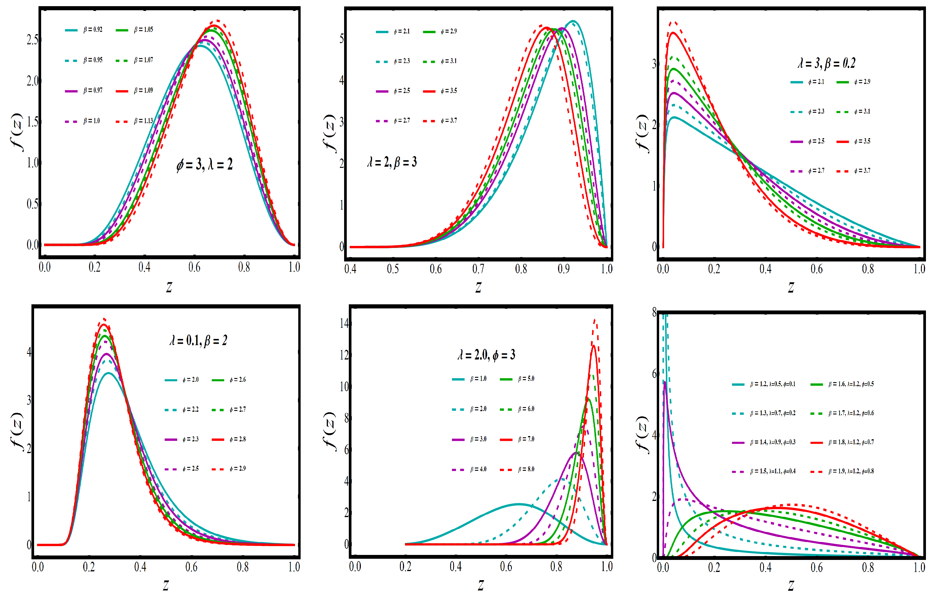
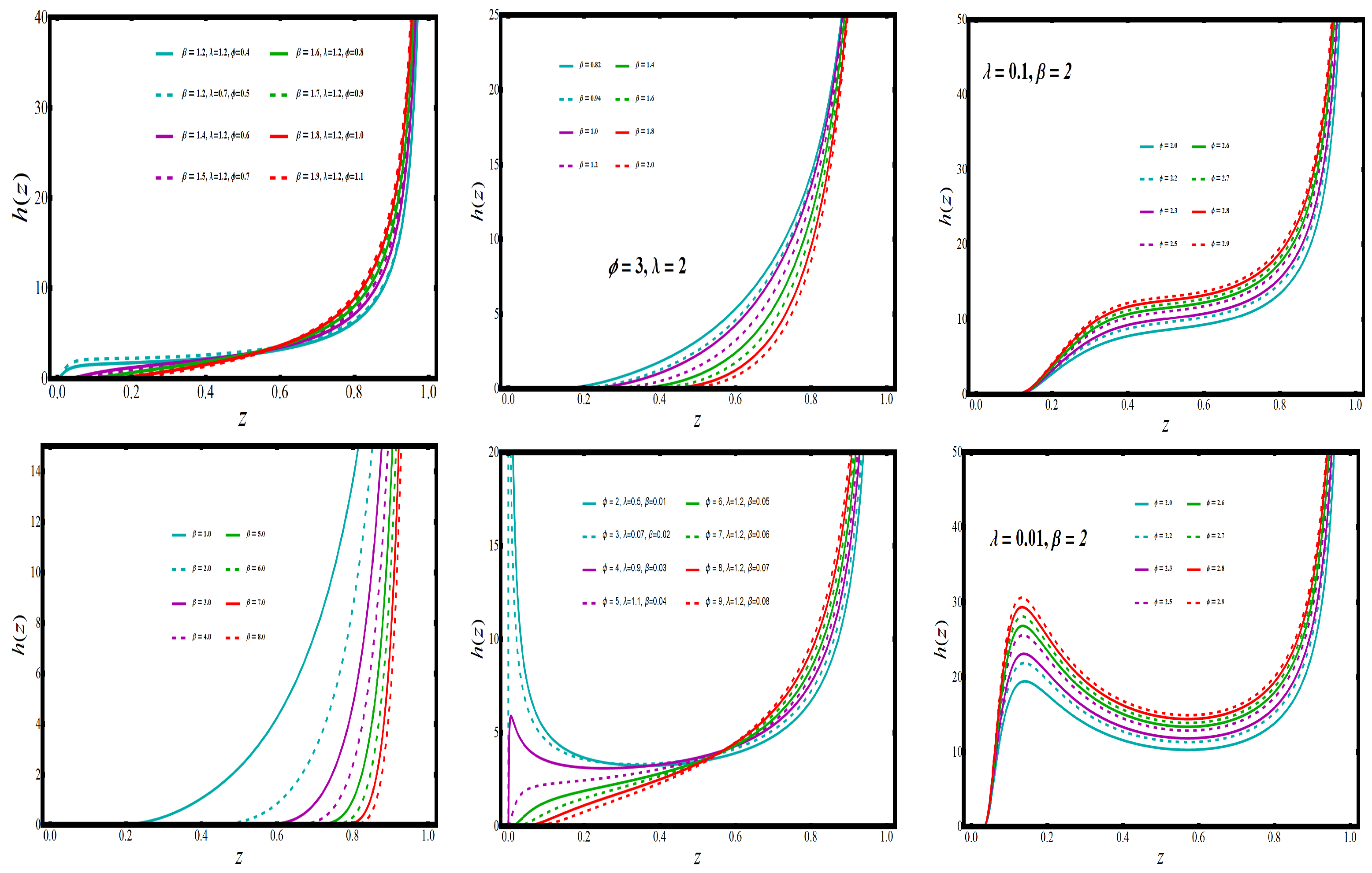
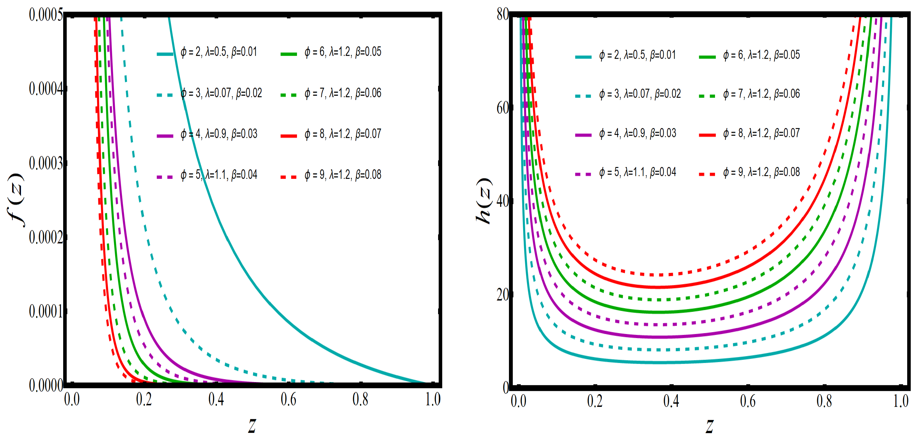
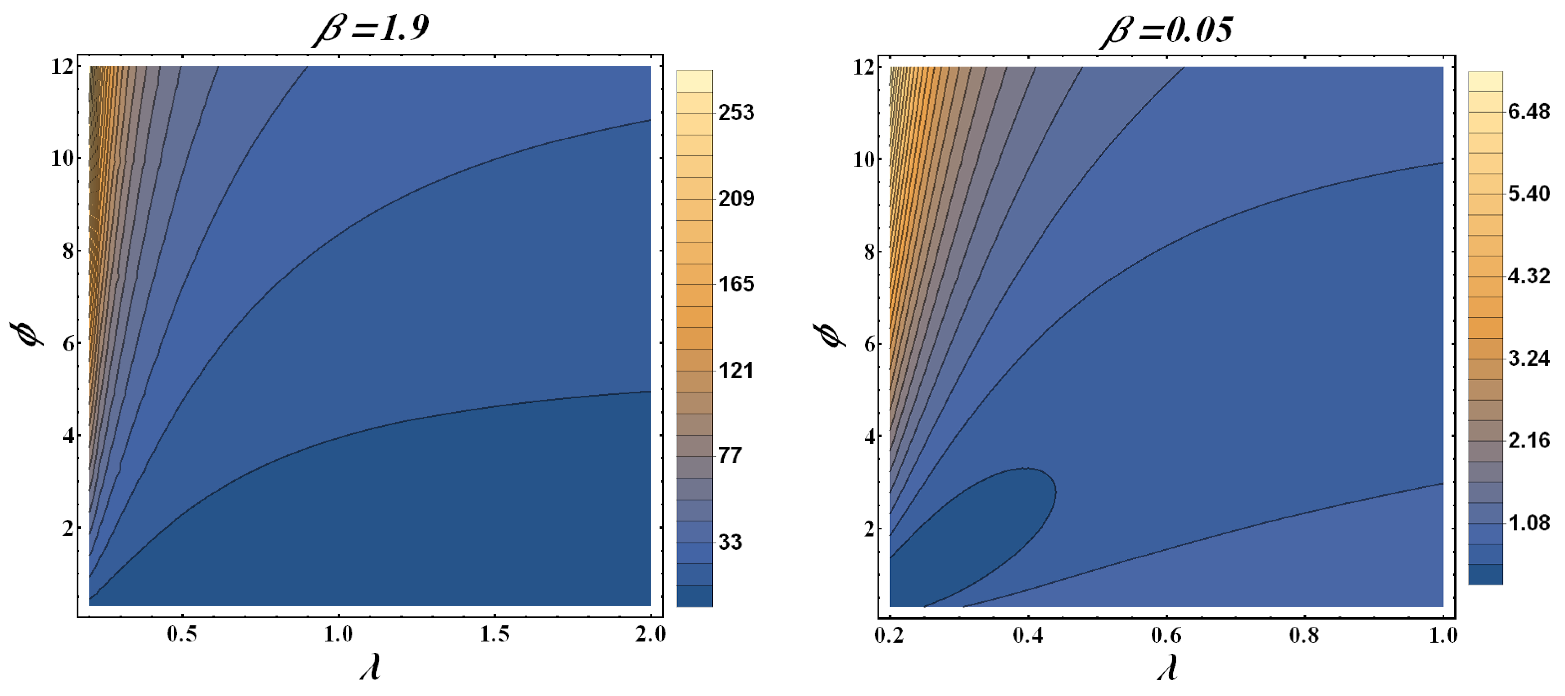
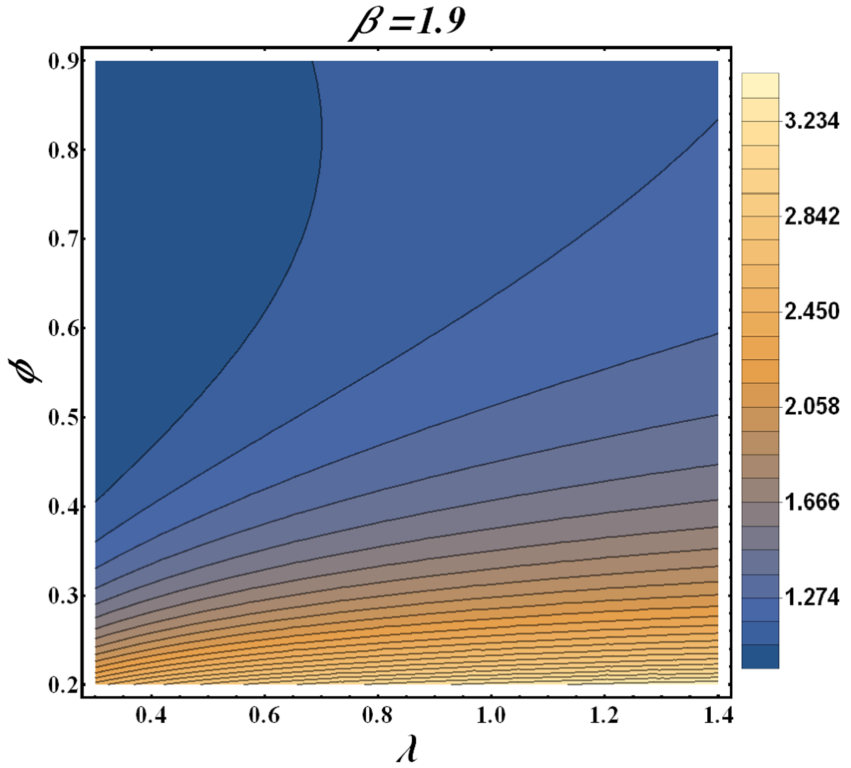
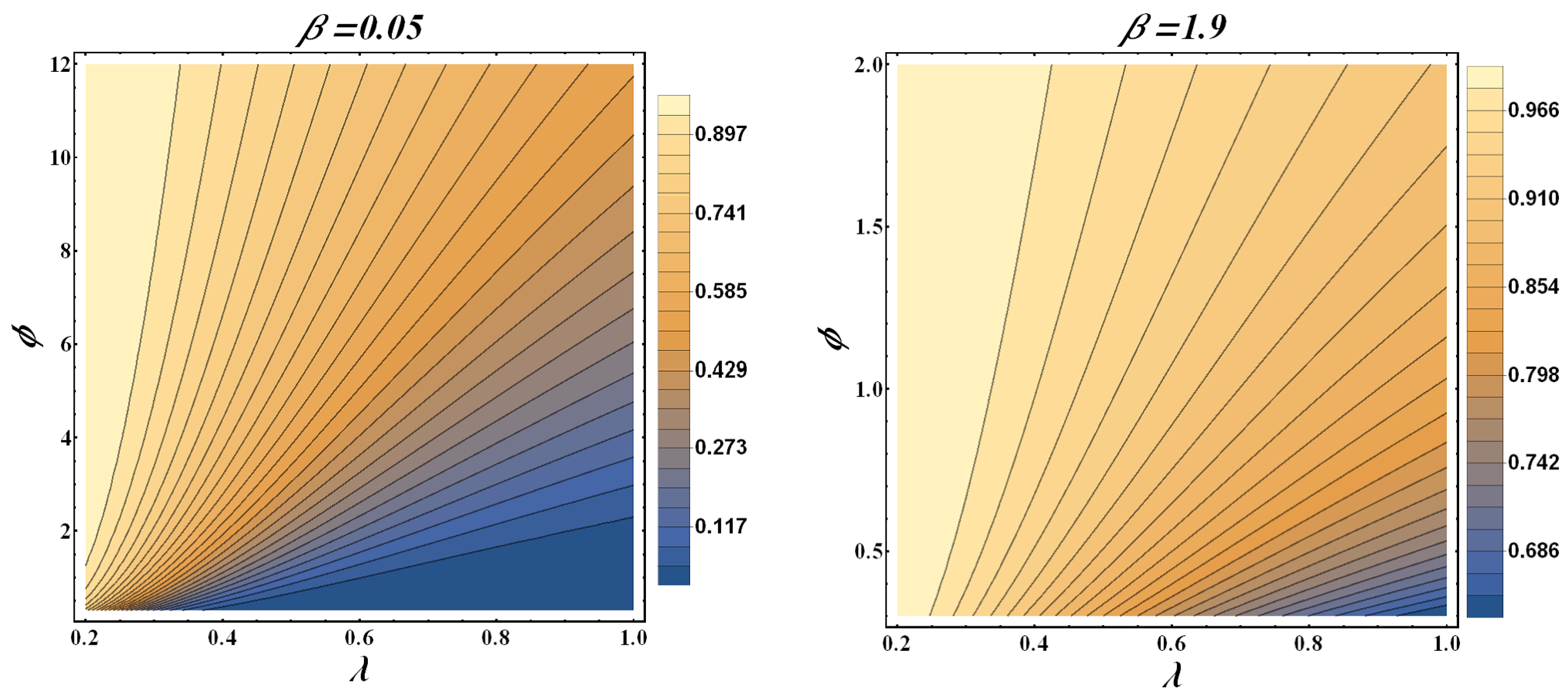
The increasing, bathtub, and upside-down forms of the HRF are shown in Figure 2. When the PDF has a monotonic decreasing trend, the HRF has a bathtub trend, which can be observed in Figure 3. Real-time applications frequently require both monotonic and non-monotonic hazard rate trends, so these versatile HRF forms are ideal. In any lifetime model, inverted bathtub curves and increasing and decreasing HRF are attractive characteristics that can be incorporated into the model.

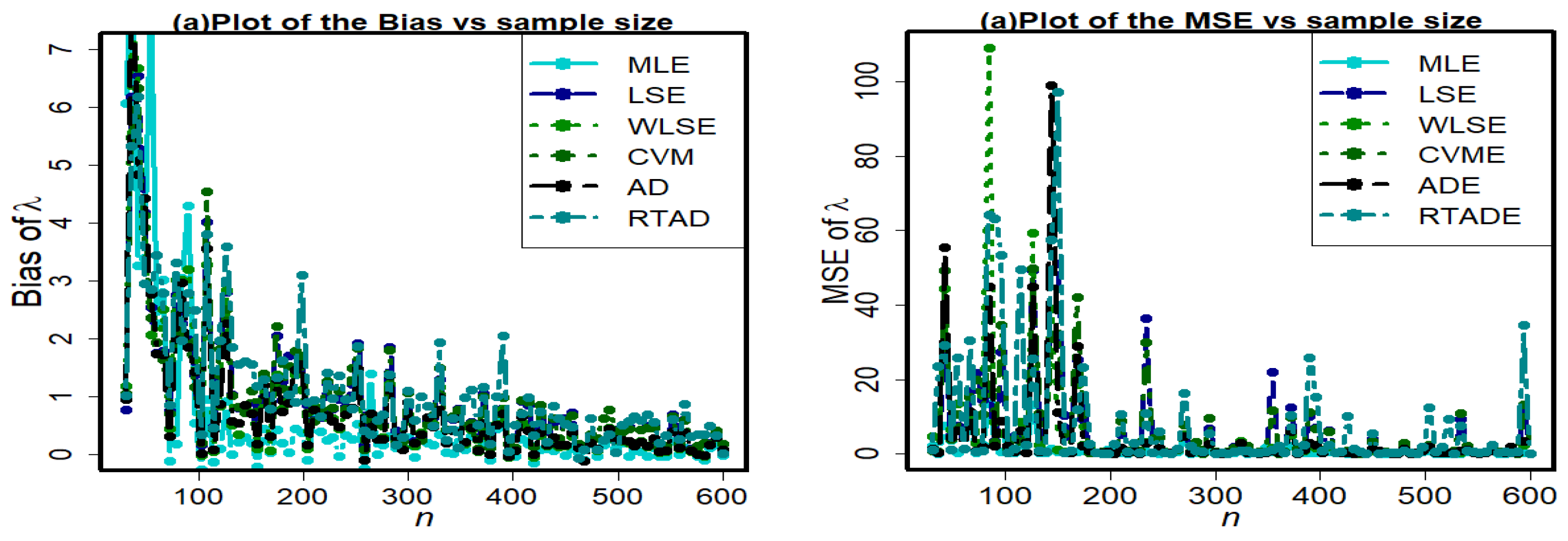
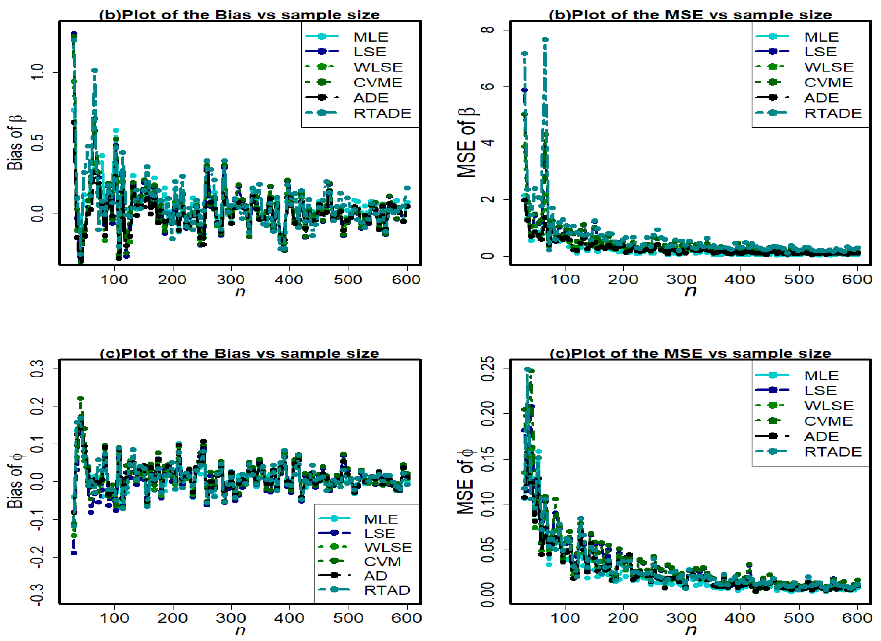
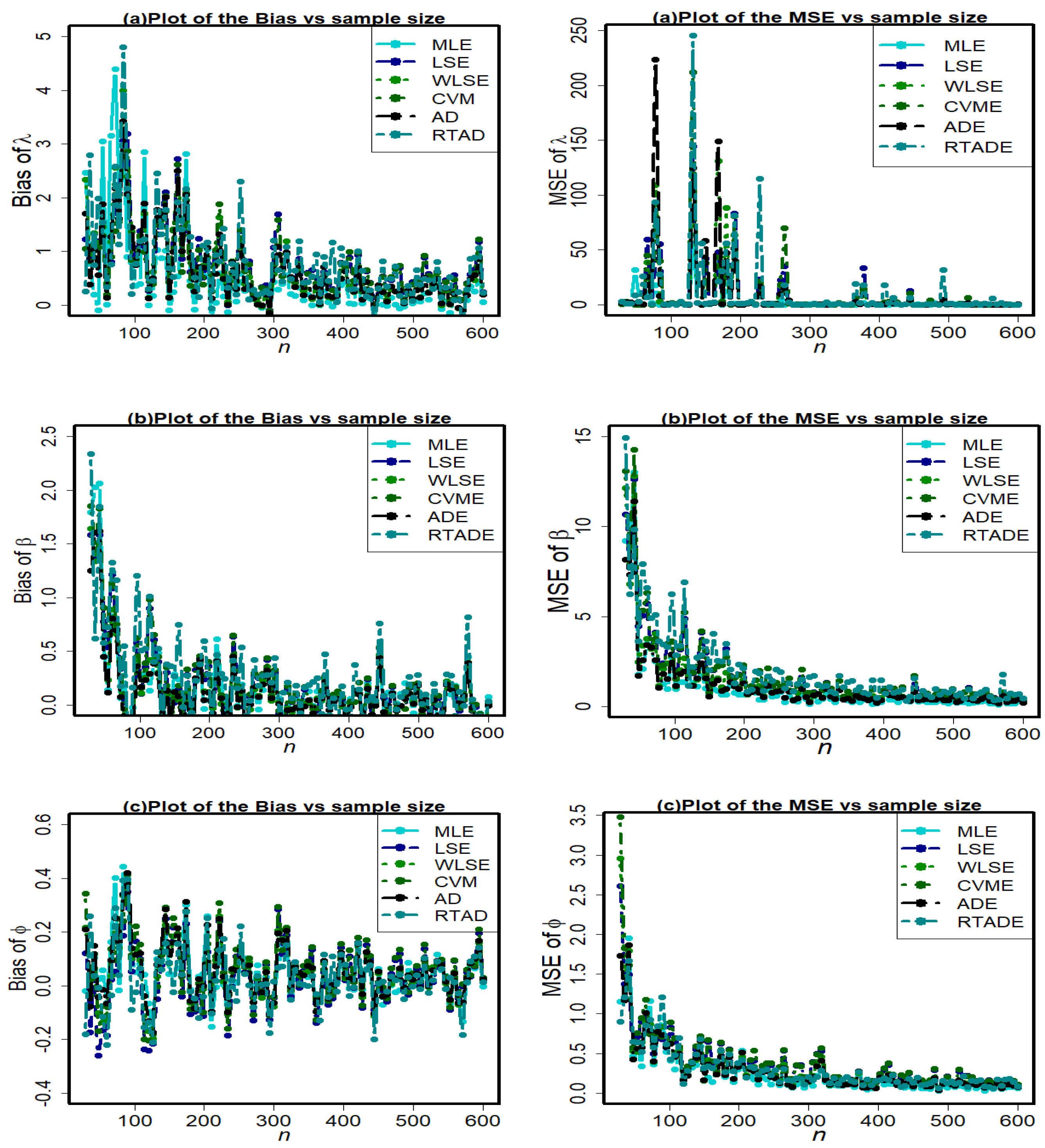
4. Statistical and Mathematical Characteristics

4.1. Quantile Function (QF)

The QF also determines the characteristics of the probability distribution, such as the moments. Furthermore, the quantile function describes the model and can be used as an alternative mechanism for data analysis [15]. Assume $G(Q_p;$ $\breve{\mathsf{\Theta }})$ is the HLUG-TI distribution’s CDF at p^th quantiles $Q_p$. Then the p^th quantile of the HLUG-TI random variable is

$$Q(p;\breve{\mathsf{\Theta }})={\left[1-\frac{1}{\lambda }log\left[1-{\left(\frac{1-p}{1+p}\right)}^{\frac{1}{\varphi }}\right]\right]}^{\frac{-1}{\beta }},0<p<1.$$

(17)

$\tilde{Z}=Q(0.5;\breve{\mathsf{\Theta }})$ shows the median of Z. There is a similar explanation for the other partition values. In particular, by setting $p=\left(0.25,0.75\right)$ in Equation (17), the first, and third quartiles are obtained. The associated quantile density function is obtained by differentiating $Q(p;\breve{\mathsf{\Theta }})$:

$$\begin{array}{ccc}\hfill Q^{\prime }(p;\breve{\mathsf{\Theta }})& =& -\frac{2}{{(1+u)}^2\beta \lambda \varphi }{\left(\frac{1-p}{1+p}\right)}^{\frac{1}{\varphi }-1}{\left[1-\frac{1}{\lambda }log\left\{1-{\left(\frac{1-p}{1+p}\right)}^{\frac{1}{\varphi }}\right\}\right]}^{-\left(\frac{\beta +1}{\beta }\right)}\hfill \\ & & {\left[{\left(\frac{1-p}{1+p}\right)}^{\frac{1}{\varphi }}-1\right]}^{-1}.\hfill \end{array}$$

(18)

At various levels of $\beta$ and different values of model parameters $\varphi$ and $\lambda$, Figure 4 shows maps of skewness, kurtosis and median. The model is discovered to be leptokurtic to platykurtic in nature and positively skewed. As $\varphi$ and $\lambda$ rise, the skewness becomes approximately equal to 2.3 at the first level of $\beta$. The skewness is higher at lower $\varphi$ and a higher value of $\lambda .$ Furthermore, the distribution peakedness yields higher values at lower $\varphi$ and $\lambda$, but as $\varphi$ and $\lambda$ increase, it ends up being roughly 1.5. Additionally, the median yields lower values at lower $\varphi$ and $\lambda$, but as $\varphi$ and $\lambda$ rise, it approaches 1.

Partition measures can be used to assess the variability of the kurtosis and skewness of Z using partition measures. Bowley’s skewness is as follows:

$$S_{\breve{\mathsf{\Theta }}}=\frac{Q\left(0.75;\breve{\mathsf{\Theta }}\right)-2Q\left(0.5;\breve{\mathsf{\Theta }}\right)+Q\left(0.25;\breve{\mathsf{\Theta }}\right)}{IQR},$$

(19)

and kurtosis is

$$K_{\breve{\mathsf{\Theta }}}=\frac{Q\left(0.875;\breve{\mathsf{\Theta }}\right)-Q\left(0.625;\breve{\mathsf{\Theta }}\right)+Q\left(0.375;\breve{\mathsf{\Theta }}\right)-Q\left(0.125;\breve{\mathsf{\Theta }}\right)}{IQR}.$$

(20)

A contour map typically shows a bunch of lines, often wavy or forming concentric, irregular closed loops or other patterns. Each of these lines, called a contour or contour line, is simply a line along which some quantity (for example, wind speed temperature) is everywhere the same. Contour graphs are plotted for skewness and median behavior in comparison to HLUG-TI distribution and the pertinent parameter values in Figure 5, Figure 6 and Figure 7 for various values of $\beta$. It is observed that skewness increases at higher values of $\varphi$ but lower levels of $\lambda$ for both $\beta =0.05,1.9$ (see Figure 5). Furthermore, in Figure 5, it is noted that lower skewness occurs near all levels of $\lambda$ and lower levels of $\varphi$. Figure 6 demonstrates that for lower levels of $\varphi$ and all levels of $\lambda ,$ kurtosis is increased, whereas for all levels of $\lambda$ and higher values of $\varphi ,$ it declines. Furthermore, when $0.4\le \varphi \le 0.9,$ and $0\le \lambda \le 0.6,$ kurtosis is decreased. Moreover, in Figure 6 for all levels of $\lambda$, $0\le \varphi \le 1$ and $\varphi \ge 4$, the kurtosis declines, whereas for lower levels of $\lambda ,$ and $0.8\le \varphi \le 2.3,$ the kurtosis increases. Figure 7 shows plotted contour graphs for the median of the HLUG-TI distribution for various values of pertinent parameters. It is noted that for higher levels of parameters $\varphi$ and $\lambda$, the median is increased, whereas it declines for lower values of parameters $\varphi$ and higher levels of $\lambda$. On the other side, a similar trend is noted for $\beta =1.9$ (see Figure 7).

4.2. Ordinary Moments

For $\breve{\mathsf{\Theta }}>0,$ by replacing (13) with the description of the $s^{th}$ moment of random variable Z. Thus,

$${\acute{\mu }}_s=E\left(Z^s\right)=\underset{0}{\overset{1}{\int }}{z}^{s}d{F}_Z(z;\breve{\mathsf{\Theta }});s=1,2\dots$$

(21)

The integral in (21) can be assessed by any computational software. An equivalent expression is given with a probable precision gain in terms of errors while using Remark 1:

$${\acute{\mu }}_s=\underset{0}{\overset{1}{\int }}{z}^s\sum _{w=0}^{+\infty }\sum _{r=1}^{+\infty }{\Lambda }_{w,r}{g}_r\left(z\right)dz,$$

(22)

where $g_r\left(z\right)=r\beta \lambda z^{-\beta -1}{e}^{\lambda r\left(1-z^{-\beta }\right)}.$ Let $\lambda r{z}^{-\beta }=t$, then $r\beta \lambda z^{-\beta -1}dz=-dt$ and after some algebraic manipulation, we have

$${\acute{\mu }}_s=\sum _{w=0}^{+\infty }\sum _{r=1}^{+\infty }{\left(\lambda r\right)}^{\frac{s}{\beta }}{\Lambda }_{w,r}{e}^{\lambda r}\Gamma \left(1-\frac{s}{\beta },\lambda r\right),$$

(23)

where $\Gamma \left(\tau ,x\right)=\underset{x}{\overset{\infty }{\int }}{y}^{\tau -1}{e}^{-y}dy$ is an incomplete gamma function. An alternative expression of ${\acute{\mu }}_s$ in terms of exponential integral is given by

$${\acute{\mu }}_s=\sum _{w=0}^{+\infty }\sum _{r=1}^{+\infty }{e}^{\lambda r}\lambda r{\Lambda }_{w,r}{E}_{\frac{s}{\beta }}\left(\lambda r\right),$$

(24)

where $E_n\left(x\right)=x^{n-1}\Gamma \left(1-n,x\right).$ The mean and variance of Z can be defined as ${\mu }_z={\acute{\mu }}_1$ and ${\sigma }_z^2={\acute{\mu }}_2-{\mu }_z^2,$ respectively, i.e.,

$${\mu }_z=\sum _{w=0}^{+\infty }\sum _{r=1}^{+\infty }{\left(\lambda r\right)}^{\frac{1}{\beta }}{e}^{\lambda r}{\Lambda }_{w,r}\Gamma \left(1-\frac{1}{\beta },\lambda r\right),$$

(25)

Additionally, in terms of the exponential integral, we have

$${\mu }_z=\sum _{w=0}^{+\infty }\sum _{r=1}^{+\infty }{e}^{\lambda r}\lambda r{\Lambda }_{w,r}{E}_{\frac{1}{\beta }}\left(\lambda r\right).$$

(26)

Therefore,

$${\sigma }_z^2=\sum _{w=0}^{+\infty }\sum _{r=1}^{+\infty }{\left(\lambda r\right)}^{\frac{2}{\beta }}{e}^{\lambda r}{\Lambda }_{w,r}\Gamma \left(1-\frac{2}{\beta },\lambda r\right)-{\left({\mu }_z\right)}^2.$$

(27)

Numerical values for some moments, skewness, variance, and kurtosis of Z for various values of the considered parameters are reported in

Table 1. Some moments, variance, skewness and kurtosis of Z for different parametric values.

$\left(\mathit{\beta },\mathit{\lambda },\mathit{\varphi }\right)$	$\left(3,2,2\right)$	$\left(2,2,2\right)$	$\left(3,3,2\right)$	$\left(4,3,5\right)$	$\left(2,7,3\right)$	$\left(0.6,1.7,7\right)$
E$\left(Z\right)$	0.87516	0.82088	0.90743	0.89166	0.91499	0.29191
E$\left(Z^2\right)$	0.77125	0.68403	0.82689	0.79691	0.83961	0.09797
E$\left(Z^3\right)$	0.68403	0.57754	0.75642	0.71382	0.77248	0.03674
E$\left(Z^4\right)$	0.61022	0.49330	0.69444	0.64077	0.71249	0.01510
${\sigma }_Z^2$	0.00535	0.01018	0.00346	0.00186	0.00239	0.01275
S	8.67374	5.77620	11.6341	15.6444	14.7932	1.86490
K	1.20946	1.19683	1.23356	1.24648	1.26732	1.21331

. Table 1 reveals that for higher values of $\beta$, by keeping $\lambda$ and $\varphi$ fixed, the first four moments about origin, skewness and kurtosis are increased, while the variance exhibits the opposite behavior.

4.3. Moment Generating Function (mgf)

The mgf is frequently used to describe models. The HLUG-TI mgf is described as

$$M\left(\left.z\right|\breve{\mathsf{\Theta }}\right)=E\left(e^{tz}\right)=\sum _{s=0}^{+\infty }\frac{t^s}{s!}{\acute{\mu }}_s=\sum _{s,w=0}^{+\infty }\sum _{r=1}^{+\infty }\frac{t^s}{s!}{\left(\lambda r\right)}^{\frac{s}{\beta }}{e}^{\lambda r}{\Lambda }_{w,r}\Gamma \left(1-\frac{s}{\beta },\lambda r\right).$$

(28)

4.4. Incomplete Noncentral Moments

Incomplete noncentral moments play a significant role in determining inequality, including the revenue quantities and curves of Lorenz and Bonferroni, which are based on incomplete distribution moments.

The definition of the upper incomplete gamma function denoted by $\Gamma \left(\varrho ,x\right)$ is

$$\Gamma \left(\varrho ,x\right)=\underset{x}{\overset{\infty }{\int }}{u}^{\varrho -1}{e}^{-u}du,x>0,\varrho \in \mathbb{R}.$$

(29)

Additionally, the upper incomplete gamma function can be given using the exponential integral function as follows (cf. Olver et al. [16]):

$$\begin{array}{ccc}\hfill E_{\hslash }\left(x\right)& =& \underset{1}{\overset{\infty }{\int }}{t}^{-\hslash }{e}^{-tx}dt,x>0,\hslash \in \mathbb{R},\hfill \\ \hfill E_{\hslash }\left(x\right)& =& x^{\hslash -1}\Gamma \left(1-\hslash ,x\right),x,\hslash \in \mathbb{R}.\hfill \end{array}$$

(30)

The $s^{th}$ incomplete moment ${\acute{\mu }}_{Z,s}\left(\nu \right)$ of Z is

$${\acute{\mu }}_{Z,s}\left(\nu \right)=\underset{0}{\overset{\nu }{\int }}{z}^{s}d{F}_Z\left(\left.z\right|\breve{\mathsf{\Theta }}\right);s=1,2,\dots$$

(31)

Let $\lambda r{z}^{-\beta }=t$, then $r\beta \lambda z^{-\beta -1}dz=-dt$, and we obtain the following simplified form:

$${\acute{\mu }}_{Z,s}\left(\nu \right)=\sum _{w=0}^{+\infty }\sum _{r=1}^{+\infty }{\left(\lambda r\right)}^{\frac{s}{\beta }}{e}^{\lambda r}{\Lambda }_{w,r}\Gamma \left(1-\frac{s}{\beta },\frac{\lambda r}{{\nu }^{\beta }}\right),$$

(32)

and in terms of the exponential integral function, we have

$${\acute{\mu }}_{Z,s}\left(\nu \right)=\sum _{w=0}^{+\infty }\sum _{r=1}^{+\infty }\lambda r{e}^{\lambda r}{\Lambda }_{w,r}{\nu }^{s-\frac{1}{\beta }}{E}_{\frac{s}{\beta }}\left(\frac{\lambda r}{{\nu }^{\beta }}\right).$$

(33)

Furthermore, the extent of variation in a data may be assessed to some extent by all deviations from $\mu$ and $\tilde{Z}$:

$${\Delta }_Z=\underset{0}{\overset{1}{\int }}\left|z-\mu \right|f\left(z\right)dz=2\mu F\left(\mu \right)-2{\acute{\mu }}_{Z,1}\left(\mu \right).$$

(34)

The mean deviations of Z about median $\tilde{Z}$ can be expressed as

$${\Psi }_Z=\underset{0}{\overset{1}{\int }}\left|z-\tilde{Z}\right|f\left(z\right)dz=\mu -2{\acute{\mu }}_{Z,1}\left(\tilde{Z}\right).$$

(35)

The Bonferroni curve is given by

$$\tilde{B}\left(q\right)=\frac{1}{q\mu }{\acute{\mu }}_{Z,1}Q(q;\breve{\mathsf{\Theta }})=\frac{1}{q\mu }{\acute{\mu }}_{Z,1}{\left[1-\frac{1}{\lambda }log\left[1-{\left(\frac{1-q}{1-q}\right)}^{\frac{1}{\varphi }}\right]\right]}^{\frac{-1}{\beta }},0<q<1,$$

(36)

where the Lorenz curves is given as

$$\tilde{L}\left(q\right)=q\tilde{B}\left(q\right),0<q<1.$$

(37)

4.5. Central Moments

The $s^{th}$ central moment of HLUG-TI$\left(\breve{\mathsf{\Theta }}\right)$ is obtained as

$${\mu }_s=\sum _{j=0}^{\infty }\left(\genfrac{}{}{0pt}{}{s}{j}\right){\left(-1\right)}^j{\mu }^j\underset{0}{\overset{1}{\int }}{z}^{s-j}d{F}_Z\left(\left.z\right|\breve{\mathsf{\Theta }}\right);$$

(38)

$${\mu }_s=\sum _{j=0}^{+\infty }\sum _{w=0}^{+\infty }\sum _{r=1}^{+\infty }\left(\genfrac{}{}{0pt}{}{s}{j}\right){\left(-1\right)}^j{\mu }^j{\left(\lambda r\right)}^{\frac{s-j}{\beta }}{e}^{\lambda r}{\Lambda }_{w,r}\Gamma \left(1-\frac{\left(s-j\right)}{\beta },\lambda r\right).$$

(39)

4.6. Characteristic Function (CF)

The CF of Z can be assessed as

$$\mathsf{\Phi }\left(\left.\tau z\right|\breve{\mathsf{\Theta }}\right)=\underset{0}{\overset{1}{\int }}{e}^{i\tau z}d{F}_Z\left(\left.z\right|\breve{\mathsf{\Theta }}\right).$$

(40)

Appplying Taylor expansion on $e^{i\tau z},$ we have

$$\mathsf{\Phi }\left(\left.\tau z\right|\breve{\mathsf{\Theta }}\right)=\sum _{s=0}^{+\infty }\frac{{\left(i\tau \right)}^s}{s!}\underset{0}{\overset{1}{\int }}{z}^{s}d{F}_Z\left(\left.z\right|\breve{\mathsf{\Theta }}\right).$$

(41)

Utilizing Equation (23), we are able to derive the characteristic function of HLUG-TI$\left(\varphi ,\mathsf{\Theta }\right)$ as follows:

$$\mathsf{\Phi }\left(\left.\tau z\right|\breve{\mathsf{\Theta }}\right)=\sum _{s,w=0}^{+\infty }\sum _{r=1}^{+\infty }\frac{{\left(i\tau \right)}^s}{s!}{\left(\lambda r\right)}^{\frac{s}{\beta }}{\Lambda }_{w,r}{e}^{\lambda r}\Gamma \left(1-\frac{s}{\beta },\lambda r\right).$$

(42)

4.7. Factorial Generating Function (FGF)

FGF of HLUG-TI$\left(\breve{\mathsf{\Theta }}\right)$ is attained as

$$\begin{array}{ccc}\hfill \Psi \left(\left.\tau z\right|\breve{\mathsf{\Theta }}\right)& =& \underset{0}{\overset{1}{\int }}{e}^{log{\left(1+\tau \right)}^z}d{F}_Z\left(\left.z\right|\breve{\mathsf{\Theta }}\right)\hfill \\ & =& \sum _{s=0}^{+\infty }\frac{{\left(log\left(1+\tau \right)\right)}^s}{s!}\underset{0}{\overset{1}{\int }}{z}^{s}d{F}_Z\left(\left.z\right|\breve{\mathsf{\Theta }}\right),\hfill \end{array}$$

(43)

$$\begin{array}{ccc}& =& \sum _{s=0}^{+\infty }\frac{{\left(log\left(1+\tau \right)\right)}^s}{s!}\underset{0}{\overset{1}{\int }}{z}^{s}d{F}_Z\left(\left.z\right|\breve{\mathsf{\Theta }}\right).\hfill \end{array}$$

(44)

Using (23), the FGF of HLUG-TI$\left(\breve{\mathsf{\Theta }}\right)$ is taken in the form

$$\Psi \left(\left.\tau z\right|\breve{\mathsf{\Theta }}\right)=\sum _{s,w=0}^{+\infty }\sum _{r=1}^{+\infty }\frac{{\left(log\left(1+\tau \right)\right)}^s}{s!}\left[{\left(\lambda r\right)}^{\frac{s}{\beta }}{\Lambda }_{w,r}{e}^{\lambda r}\Gamma \left(1-\frac{s}{\beta },\lambda r\right)\right].$$

(45)

4.8. Order Statistics (ODS)

The first discussion of order statistics (ODS) from the perspective of the standard normal distribution appeared in Tippett [17]. It is continually expanding in scope to model a wide range of phenomena, typically in reliability analysis and life testing. In this section, we present some insightful results about the ODS of HLUG-TI ($\breve{\mathsf{\Theta }}$) model. Suppose $Z_{\left(1\right)}\le Z_{\left(2\right)}\dots \le Z_{\left(n\right)}$ be ODS of a random sample size n from model $G\left(z\right).$ Consequently, for $m=1,2,\dots ,n,$ the PDF of $m^{th}$ ODS, $Z_{\left(m\right)}$ is

$$g_{\left(m\right)}\left(\left.z\right|\breve{\mathsf{\Theta }}\right)=\tilde{K}G{\left(\left.z\right|\breve{\mathsf{\Theta }}\right)}^{m-1}{\left\{1-G\left(\left.z\right|\breve{\mathsf{\Theta }}\right)\right\}}^{n-m}g\left(\left.z\right|\breve{\mathsf{\Theta }}\right),$$

(46)

where $\tilde{K}=\frac{n!}{\left(m-1\right)!\left(n-m\right)!}.$ Therefore, the PDF of $m^{th}$ ODS is attained via putting Equations (13), (14) and (46), changing a with $f+m-1$:

$$g_{\left(m\right)}\left(\left.z\right|\breve{\mathsf{\Theta }}\right)=\widehat{\Psi }\sum _{r=1}^{+\infty }\sum _{k=0}^{f+m-1}\sum _{w,l,m_1}^{+\infty }{\Lambda }_{f+m-1,k,m_1}{\Delta }_{m_1}\left(z\right){\Lambda }_{w,r}{g}_r\left(z\right),$$

(47)

where

$$\begin{array}{ccc}\hfill \widehat{\Psi }& =& \tilde{K}\sum _{f=0}^{n-m}\left(\genfrac{}{}{0pt}{}{n-m}{f}\right){\left(-1\right)}^f,\hfill \\ \hfill {\Lambda }_{f+m-1,k,m_1}& =& \left(\genfrac{}{}{0pt}{}{f+m-1}{k}\right){\left(-1\right)}^{f+m-1+k+l+m_1}{2}^k\frac{\Gamma \left(l+k\right)}{l!\Gamma \left(k\right)}\frac{\Gamma \left(\varphi l+1\right)}{m_1!\Gamma \left(\varphi l+1-m_1\right)}{\Lambda }_{w,r},\hfill \end{array}$$

and ${\Delta }_{m_1}\left(z\right)=exp\left\{-\lambda m_1\left(z^{-\beta }-1\right)\right\}.$ The CDF of $Z_{\left(m\right)}$ is

$$G_{\left(m\right)}\left(\left.z\right|\varphi ,\mathsf{\Theta }\right)=\sum _{j=m}^n\left(\genfrac{}{}{0pt}{}{n}{j}\right)G{\left(\left.z\right|\varphi ,\mathsf{\Theta }\right)}^j{\left\{1-G\left(\left.z\right|\varphi ,\mathsf{\Theta }\right)\right\}}^{n-j}.$$

(48)

Thus, the CDF of $m^{th}$ ODS, $Z_{\left(m\right)}$ of HLUG-TI ($\breve{\mathsf{\Theta }}$) is

$$G_{\left(m\right)}\left(\left.z\right|\varphi ,\mathsf{\Theta }\right)=\mathsf{\Phi }\sum _{k=0}^{p+j}\sum _{l,m_1}^{+\infty }{\Lambda }_{p+j,k,m_1}{\Delta }_{m_1}\left(z\right),$$

(49)

where $\mathsf{\Phi }={\displaystyle \sum _{j=m}^n}{\displaystyle \sum _{p=0}^{n-j}}{\left(-1\right)}^p\left(\genfrac{}{}{0pt}{}{n-j}{p}\right)\left(\genfrac{}{}{0pt}{}{n}{j}\right),$ and ${\Lambda }_{p+j,k,m_1}={\left(-1\right)}^{p+j+k+l+m_1}\left(\genfrac{}{}{0pt}{}{p+j}{k}\right)2^k\frac{\Gamma \left(\varphi l+1\right)}{m_1!\Gamma \left(\varphi l+1-m_1\right)}$

$\frac{\Gamma \left(l+k\right)}{l!\Gamma \left(k\right)}$. Specifically, the CDFs of $Z_{\left(n\right)}$ and $Z_{\left(1\right)}$ are obtain, respectively as

$$G_{\left(n\right)}\left(z\right)=G^n\left(z\right),G_{\left(1\right)}\left(z\right)=1-{\left[1-G\left(z\right)\right]}^n,$$

(50)

where $G\left(.\right)$ is given in (12):

$$G_{\left(n\right)}\left(\left.z\right|\breve{\mathsf{\Theta }}\right)=\sum _{k=0}^n\sum _{l,m_1}^{+\infty }{\Lambda }_{n,k,m_1}{\Delta }_{m_1}\left(z\right),$$

(51)

$$G_{\left(1\right)}\left(\left.z\right|\breve{\mathsf{\Theta }}\right)=1-2^n{\left(1-\sum _{w=0}^{+\infty }\sum _{r=0}^{+\infty }{\Lambda }_{w,r}{F}^r(z;\breve{\mathsf{\Theta }})\right)}^n.$$

(52)

Let $Q_{\left(m\right)}\left(q\right)$ be (for $0<q<1)$ the QF of $Z_{\left(m\right)}$. Then from $\left(39\right)$, we obtain

$$Q_{\left(n\right)}\left(q\right)=Q\left(q^{1/n}\right),Q_{\left(1\right)}\left(q\right)=Q\left\{1-{\left[1-q\right]}^{1/n}\right\},$$

(53)

where $Q\left(.\right)$ is QF of $Z.$ Therefore, from $\left(17\right)$ and $\left(53\right)$, the qfs of $Z_{\left(n\right)}$ and $Z_{\left(1\right)}$ are in closed-form. For the independent and identically random variable, it is possible to determine the equation for the $s^{th}$ ordinary moment of ODS when ${\acute{\mu }}_s<\infty$. Thus, we can define the $s^{th}$ moment of $m^{th}$ ODS $Z_{\left(m\right)}$ as (see [18])

$${\mu }_{\left(m\right)}^s=Ę\left\{Z_{\left(m\right)}^s\right\}=\sum _{j=n-m+1}^n\left(\genfrac{}{}{0pt}{}{n}{j}\right)\left(\genfrac{}{}{0pt}{}{j-1}{n-m}\right){\left(-1\right)}^{j-n+m-1}{Į}_j\left(s\right),$$

(54)

where Į${}_j\left(s\right)=s\underset{0}{\overset{1}{\int }}{z}^{s-1}{\left[1-G\left(\left.z\right|\breve{\mathsf{\Theta }}\right)\right]}^{j}dz.$

In particular, for the HLUG-TI$\left(\breve{\mathsf{\Theta }}\right)$, we obtain

$${Į}_j\left(s\right)=s\sum _{j=n-m+1}^n\left(\genfrac{}{}{0pt}{}{n}{j}\right)\left(\genfrac{}{}{0pt}{}{j-1}{n-m}\right){\left(-1\right)}^{j-n+m-1}\underset{0}{\overset{1}{\int }}{z}^{s-1}{\left[1-G\left(\left.z\right|\breve{\mathsf{\Theta }}\right)\right]}^{j}dz,$$

(55)

where the final integral can be numerically evaluated.

5. Parameter Estimation with Simulation

This section examines the estimation of $\breve{\mathsf{\Theta }}$ using the six various approaches indicated in the introduction section while using the HLUG-TI ($\breve{\mathsf{\Theta }}$) distribution as a statistical model. From now, $z_1,z_2,\dots ,z_n$ show n observed values from Z, with their values in ascending order $z_{\left(1\right)}\le z_{\left(2\right)}\le \dots \le z_{\left(n\right)}.$

5.1. Maximum Likelihood Estimators

Let $z_1,z_2,\dots ,z_n$ show n observed values from the HLUG-TI ($\breve{\mathsf{\Theta }}$) distribution. Then, MLEs can be determined by maximizing the following function:

$$\begin{array}{ccc}\hfill l\left(\left.\mathbf{z}\right|\breve{\mathsf{\Theta }}\right)& =& nlog2+nlog\varphi +nlog\beta +nlog\lambda -\left(\beta +1\right)\sum _{i=1}^{n}log{z}_i-\lambda \sum _{i=1}^n\left(z_i^{-\beta }-1\right)\hfill \\ & & +\left(\varphi -1\right)\sum _{i=1}^{n}log\left[1-exp\left\{-\lambda \left(z_i^{-\beta }-1\right)\right\}\right]\hfill \\ & & -2\sum _{i=1}^{n}log\left\{1+{\left[1-exp\left\{-\lambda \left(z_i^{-\beta }-1\right)\right\}\right]}^{\varphi }\right\},\hfill \end{array}$$

(56)

Therefore, the MLEs are created by simultaneously solving the following equations $\partial l\left(\left.\mathbf{z}\right|\breve{\mathsf{\Theta }}\right)/\partial \varphi =0,$ $\partial l\left(\left.\mathbf{z}\right|\breve{\mathsf{\Theta }}\right)/\partial \lambda =0$ and $\partial l\left(\left.\mathbf{z}\right|\breve{\mathsf{\Theta }}\right)/\partial \beta =0$, where

$$\begin{array}{ccc}\hfill \frac{\partial l\left(\left.\mathbf{z}\right|\breve{\mathsf{\Theta }}\right)}{\partial \varphi }& =& \frac{n}{\varphi }+\sum _{i=1}^{n}log\left[1-exp\left\{-\lambda \left(z_i^{-\beta }-1\right)\right\}\right]\hfill \\ & & -2\sum _{i=1}^n\frac{{\left[1-exp\left\{-\lambda \left(z_i^{-\beta }-1\right)\right\}\right]}^{\varphi }log\left[1-exp\left\{-\lambda \left(z_i^{-\beta }-1\right)\right\}\right]}{1+{\left[1-exp\left\{-\lambda \left(z_i^{-\beta }-1\right)\right\}\right]}^{\varphi }},\hfill \end{array}$$

(57)

$$\begin{array}{ccc}\hfill \frac{\partial l\left(\left.\mathbf{z}\right|\breve{\mathsf{\Theta }}\right)}{\partial \lambda }& =& \frac{n}{\lambda }-\sum _{i=1}^n\left(z_i^{-\beta }-1\right)+\left(\varphi -1\right)\sum _{i=1}^n\frac{e^{-\lambda \left(z_i^{-\beta }-1\right)}\left(z_i^{-\beta }-1\right)}{1-exp\left\{-\lambda \left(z_i^{-\beta }-1\right)\right\}}\hfill \\ & & -2\sum _{i=1}^n\frac{\left(z_i^{-\beta }-1\right)e^{-\lambda \left(z_i^{-\beta }-1\right)}\varphi {\left[1-exp\left\{-\lambda \left(z_i^{-\beta }-1\right)\right\}\right]}^{\varphi -1}}{1+{\left[1-exp\left\{-\lambda \left(z_i^{-\beta }-1\right)\right\}\right]}^{\varphi }},\hfill \end{array}$$

(58)

and

$$\begin{array}{ccc}\hfill \frac{\partial l\left(\left.\mathbf{z}\right|\breve{\mathsf{\Theta }}\right)}{\partial \beta }& =& \frac{n}{\beta }-\sum _{i=1}^{n}log{z}_i+\lambda \sum _{i=1}^n{z}_i^{-\beta }log{z}_i-\left(\varphi -1\right)\sum _{i=1}^n\frac{\lambda z_i^{-\beta }log{z}_i{e}^{-\lambda \left(z_i^{-\beta }-1\right)}}{1-exp\left\{-\lambda \left(z_i^{-\beta }-1\right)\right\}}\hfill \\ & & +2\sum _{i=1}^n\frac{\lambda \varphi z_i^{-\beta }log{z}_i{e}^{-\lambda \left(z_i^{-\beta }-1\right)}{\left[1-exp\left\{-\lambda \left(z_i^{-\beta }-1\right)\right\}\right]}^{\varphi -1}}{1+{\left[1-exp\left\{-\lambda \left(z_i^{-\beta }-1\right)\right\}\right]}^{\varphi }}.\hfill \end{array}$$

(59)

5.2. Least Square Estimators

It is possible to minimize the following function in order to obtain the least square estimators of the unknown parameters $\breve{\mathsf{\Theta }}$ of HLUG-TI ($\breve{\mathsf{\Theta }}$) distribution:

$$\begin{array}{ccc}\hfill LS\left(\breve{\mathsf{\Theta }}\right)& =& \sum _{i=1}^n{\left[G(z_{\left(i\right)};\breve{\mathsf{\Theta }})-\frac{i}{n+1}\right]}^2,\hfill \end{array}$$

(60)

$$\begin{array}{ccc}& =& \sum _{i=1}^n{\left[\frac{1-{\left[1-exp\left\{-\lambda \left(z_{\left(i\right)}^{-\beta }-1\right)\right\}\right]}^{\varphi }}{1+{\left[1-exp\left\{-\lambda \left(z_{\left(i\right)}^{-\beta }-1\right)\right\}\right]}^{\varphi }}-\frac{i}{n+1}\right]}^2.\hfill \end{array}$$

(61)

with respect to unknown parameters $\breve{\mathsf{\Theta }}.$

The nonlinear equations can also be solved to find the least square estimators, such as $\partial LS\left(\breve{\mathsf{\Theta }}\right)/\partial \varphi =0,$ $\partial LS\left(\breve{\mathsf{\Theta }}\right)/\partial \lambda$ and $\partial LS\left(\breve{\mathsf{\Theta }}\right)/\partial \beta$ $=0,$ where

$$\frac{\partial LS\left(\breve{\mathsf{\Theta }}\right)}{\partial \varphi }=2\sum _{i=1}^n{\xi }_i^1\left(\breve{\mathsf{\Theta }}\right)\left[\frac{1-{\left[1-exp\left\{-\lambda \left(z_{\left(i\right)}^{-\beta }-1\right)\right\}\right]}^{\varphi }}{1+{\left[1-exp\left\{-\lambda \left(z_{\left(i\right)}^{-\beta }-1\right)\right\}\right]}^{\varphi }}-\frac{i}{n+1}\right],$$

(62)

$$\frac{\partial LS\left(\breve{\mathsf{\Theta }}\right)}{\partial \lambda }=2\sum _{i=1}^n{\xi }_i^2\left(\breve{\mathsf{\Theta }}\right)\left[\frac{1-{\left[1-exp\left\{-\lambda \left(z_{\left(i\right)}^{-\beta }-1\right)\right\}\right]}^{\varphi }}{1+{\left[1-exp\left\{-\lambda \left(z_{\left(i\right)}^{-\beta }-1\right)\right\}\right]}^{\varphi }}-\frac{i}{n+1}\right],$$

(63)

$$\frac{\partial LS\left(\breve{\mathsf{\Theta }}\right)}{\partial \beta }=2\sum _{i=1}^n{\xi }_i^3\left(\breve{\mathsf{\Theta }}\right)\left[\frac{1-{\left[1-exp\left\{-\lambda \left(z_{\left(i\right)}^{-\beta }-1\right)\right\}\right]}^{\varphi }}{1+{\left[1-exp\left\{-\lambda \left(z_{\left(i\right)}^{-\beta }-1\right)\right\}\right]}^{\varphi }}-\frac{i}{n+1}\right],$$

(64)

where

$${\xi }_i^1\left(\breve{\mathsf{\Theta }}\right)=-2\frac{{\left[1-e^{-\lambda \left(z_{\left(i\right)}^{-\beta }-1\right)}\right]}^{\varphi }log[1-e^{-\lambda \left(z_{\left(i\right)}^{-\beta }-1\right)}]}{{\left[1+{\left(1-e^{-\lambda \left(z_{\left(i\right)}^{-\beta }-1\right)}\right)}^{\varphi }\right]}^2},$$

(65)

$${\xi }_i^2\left(\breve{\mathsf{\Theta }}\right)=-2\frac{\varphi e^{-\lambda \left(z_{\left(i\right)}^{-\beta }-1\right)}{\left[1-e^{-\lambda \left(z_{\left(i\right)}^{-\beta }-1\right)}\right]}^{\varphi -1}\left(z_{\left(i\right)}^{-\beta }-1\right)}{{\left[1+{\left(1-e^{-\lambda \left(z_{\left(i\right)}^{-\beta }-1\right)}\right)}^{\varphi }\right]}^2},$$

(66)

$${\xi }_i^3\left(\breve{\mathsf{\Theta }}\right)=2\frac{\varphi \lambda z_{\left(i\right)}^{-\beta }log{z}_i{e}^{-\lambda \left(z_{\left(i\right)}^{-\beta }-1\right)}{\left[1-e^{-\lambda \left(z_{\left(i\right)}^{-\beta }-1\right)}\right]}^{\varphi -1}}{{\left[1+{\left(1-e^{-\lambda \left(z_{\left(i\right)}^{-\beta }-1\right)}\right)}^{\varphi }\right]}^2}.$$

(67)

5.3. Weighted Least Square Estimators

The WLSEs, ${\widehat{\varphi }}_{WLSE}$, ${\widehat{\lambda }}_{WLSE}$ and ${\widehat{\beta }}_{{}_{WLSE}}$ can be calculated by minimizing the subsequent function with respect to $\varphi ,$ $\lambda$ and $\beta$

$$\begin{array}{ccc}\hfill W\left(\breve{\mathsf{\Theta }}\right)& =& \sum _{i=1}^n\frac{(n+2){(n+1)}^2}{i(n-i+1)}{\left[G(z_{\left(i\right)};\breve{\mathsf{\Theta }})-\frac{i}{n+1}\right]}^2,\hfill \end{array}$$

(68)

$$\begin{array}{ccc}& =& \sum _{i=1}^n\frac{(n+2){(n+1)}^2}{i(n-i+1)}{\left[\frac{1-{\left[1-exp\left\{-\lambda \left(z_{\left(i\right)}^{-\beta }-1\right)\right\}\right]}^{\varphi }}{1+{\left[1-exp\left\{-\lambda \left(z_{\left(i\right)}^{-\beta }-1\right)\right\}\right]}^{\varphi }}-\frac{i}{n+1}\right]}^2.\hfill \end{array}$$

(69)

We can also obtain these estimators by solving $\partial W\left(\breve{\mathsf{\Theta }}\right)/\partial \varphi =0,$ $\partial W\left(\breve{\mathsf{\Theta }}\right)/\partial \lambda$ and $\partial W\left(\breve{\mathsf{\Theta }}\right)/\partial \beta$ $=0$, where

$$\frac{\partial W\left(\breve{\mathsf{\Theta }}\right)}{\partial \varphi }=2\sum _{i=1}^n\frac{{(n+1)}^2(n+2)}{i(n-i+1)}{\xi }_i^1\left(\mathsf{\Theta }\right)\left[\frac{1-{\left[1-exp\left\{-\lambda \left(z_{\left(i\right)}^{-\beta }-1\right)\right\}\right]}^{\varphi }}{1+{\left[1-exp\left\{-\lambda \left(z_{\left(i\right)}^{-\beta }-1\right)\right\}\right]}^{\varphi }}-\frac{i}{n+1}\right],$$

(70)

$$\frac{\partial W\left(\breve{\mathsf{\Theta }}\right)}{\partial \lambda }=2\sum _{i=1}^n\frac{{(n+1)}^2(n+2)}{i(n-i+1)}{\xi }_i^2\left(\mathsf{\Theta }\right)\left[\frac{1-{\left[1-exp\left\{-\lambda \left(z_{\left(i\right)}^{-\beta }-1\right)\right\}\right]}^{\varphi }}{1+{\left[1-exp\left\{-\lambda \left(z_{\left(i\right)}^{-\beta }-1\right)\right\}\right]}^{\varphi }}-\frac{i}{n+1}\right],$$

(71)

$$\frac{\partial W\left(\breve{\mathsf{\Theta }}\right)}{\partial \beta }=2\sum _{i=1}^n\frac{{(n+1)}^2(n+2)}{i(n-i+1)}{\xi }_i^2\left(\mathsf{\Theta }\right)\left[\frac{1-{\left[1-exp\left\{-\lambda \left(z_{\left(i\right)}^{-\beta }-1\right)\right\}\right]}^{\varphi }}{1+{\left[1-exp\left\{-\lambda \left(z_{\left(i\right)}^{-\beta }-1\right)\right\}\right]}^{\varphi }}-\frac{i}{n+1}\right],$$

(72)

where ${\xi }_i^j\left(\mathsf{\Theta }\right),$ $j=1,2,3$ are given in (65)–(67).

5.4. Cramér–von Mises Estimators

Cramér–von Mises estimators ${\widehat{\varphi }}_{CVME}$, ${\widehat{\lambda }}_{CVME}$ and ${\widehat{\beta }}_{{}_{CVME}}$ of parameters $\varphi ,$ $\lambda$ and $\beta$ can be calculated by minimizing the following function with respect to $\varphi ,$ $\lambda$ and $\beta$:

$$\begin{array}{ccc}\hfill C\left(\breve{\mathsf{\Theta }}\right)& =& \frac{1}{12n}+\sum _{i=1}^n{\left[G(z_{\left(i\right)};\breve{\mathsf{\Theta }})-\frac{2i-1}{2n}\right]}^2,\hfill \\ & =& \frac{1}{12n}+\sum _{i=1}^n{\left[\frac{1-{\left[1-exp\left\{-\lambda \left(z_{\left(i\right)}^{-\beta }-1\right)\right\}\right]}^{\varphi }}{1+{\left[1-exp\left\{-\lambda \left(z_{\left(i\right)}^{-\beta }-1\right)\right\}\right]}^{\varphi }}-\frac{2i-1}{2n}\right]}^2.\hfill \end{array}$$

(73)

To find similar estimators, the following nonlinear equations should be solved:

$$\frac{\partial C\left(\breve{\mathsf{\Theta }}\right)}{\partial \varphi }=2\sum _{i=1}^n{\xi }_i^1\left(\breve{\mathsf{\Theta }}\right)\left[\frac{1-{\left[1-exp\left\{-\lambda \left(z_{\left(i\right)}^{-\beta }-1\right)\right\}\right]}^{\varphi }}{1+{\left[1-exp\left\{-\lambda \left(z_{\left(i\right)}^{-\beta }-1\right)\right\}\right]}^{\varphi }}-\frac{2i-1}{2n}\right]=0,$$

(74)

$$\frac{\partial C\left(\breve{\mathsf{\Theta }}\right)}{\partial \lambda }=2\sum _{i=1}^n{\xi }_i^2\left(\breve{\mathsf{\Theta }}\right)\left[\frac{1-{\left[1-exp\left\{-\lambda \left(z_{\left(i\right)}^{-\beta }-1\right)\right\}\right]}^{\varphi }}{1+{\left[1-exp\left\{-\lambda \left(z_{\left(i\right)}^{-\beta }-1\right)\right\}\right]}^{\varphi }}-\frac{2i-1}{2n}\right]=0,$$

(75)

$$\frac{\partial C\left(\breve{\mathsf{\Theta }}\right)}{\partial \beta }=2\sum _{i=1}^n{\xi }_i^3\left(\breve{\mathsf{\Theta }}\right)\left[\frac{1-{\left[1-exp\left\{-\lambda \left(z_{\left(i\right)}^{-\beta }-1\right)\right\}\right]}^{\varphi }}{1+{\left[1-exp\left\{-\lambda \left(z_{\left(i\right)}^{-\beta }-1\right)\right\}\right]}^{\varphi }}-\frac{2i-1}{2n}\right]=0,$$

(76)

where ${\xi }_i^j\left(\breve{\mathsf{\Theta }}\right)$, $j=1,2,3$ are defined in (65)–(67).

5.5. ADE and RTADE Approach

Anderson and Darling [19] established the Anderson–Darling (AD) test. In particular, the AD test rapidly converges toward the asymptote ([20,21,22]). The Anderson–Darling statistic is obtained as

$$AD{S}_n^2=n{\int }_{-\infty }^{\infty }\frac{{\left[G\left(z_{\left(i\right)}\right)-G_n\left(z_{\left(i\right)}\right)\right]}^2}{G\left(z_{\left(i\right)}\right)\left(1-G\left(z_{\left(i\right)}\right)\right)}dG\left(z_{\left(i\right)}\right),$$

(77)

where $G_n\left(z_{\left(i\right)}\right)$ is the empirical distribution function and $G\left(z_{\left(i\right)}\right)$ is the cumulative distribution given in (3). Boos [23] also examined the AD estimators’ characteristics. The Anderson–Darling estimators ${\widehat{\varphi }}_{ADE}$, ${\widehat{\lambda }}_{ADE}$ and ${\widehat{\beta }}_{{}_{ADE}}$ of the parameters $\varphi ,$ $\lambda$ and $\beta$ are determined by minimizing the following function with respect to $\varphi ,$ $\lambda$ and $\beta$:

$$A\left(\breve{\mathsf{\Theta }}\right)=-n-\frac{1}{n}\sum _{i=1}^n\left(2i-1\right)\left(log\left[G(z_{\left(i\right)};\breve{\mathsf{\Theta }})\right]+log\left[\overline{G}(z_{(n+1-i)};\breve{\mathsf{\Theta }})\right]\right),$$

(78)

where $\overline{G}(.)=1-G\left(.\right).$ To find similar estimators, the following nonlinear equations should be solved:

$$\frac{\partial A\left(\breve{\mathsf{\Theta }}\right)}{\partial \varphi }=-\frac{1}{n}\sum _{i=1}^n\left(2i-1\right)\left[\frac{{\xi }_i^1\left(\breve{\mathsf{\Theta }}\right)}{G(z_{\left(i\right)};\breve{\mathsf{\Theta }})}-\frac{{\xi }_{(n+1-i)}^1\left(\breve{\mathsf{\Theta }}\right)}{\overline{G}(z_{(n+1-i)};\breve{\mathsf{\Theta }})}\right]=0,$$

(79)

$$\frac{\partial A\left(\breve{\mathsf{\Theta }}\right)}{\partial \lambda }=-\frac{1}{n}\sum _{i=1}^n\left(2i-1\right)\left[\frac{{\xi }_i^2\left(\breve{\mathsf{\Theta }}\right)}{G(z_{\left(i\right)};\breve{\mathsf{\Theta }})}-\frac{{\xi }_{(n+1-i)}^2\left(\breve{\mathsf{\Theta }}\right)}{\overline{G}(z_{(n+1-i)};\breve{\mathsf{\Theta }})}\right]=0,$$

(80)

$$\frac{\partial A\left(\breve{\mathsf{\Theta }}\right)}{\partial \beta }=-\frac{1}{n}\sum _{i=1}^n\left(2i-1\right)\left[\frac{{\xi }_i^3\left(\breve{\mathsf{\Theta }}\right)}{G(z_{\left(i\right)};\breve{\mathsf{\Theta }})}-\frac{{\xi }_{(n+1-i)}^3\left(\breve{\mathsf{\Theta }}\right)}{\overline{G}(z(n+1-i);\breve{\mathsf{\Theta }})}\right]=0,$$

(81)

where ${\xi }_i^j\left(\breve{\mathsf{\Theta }}\right)$ and $j=1,2,3$ are given in Equations (65)–(67), respectively.

The right-tail AD statistics provided by [11,17,21] are the most commonly used statistics and is given by

$$RTAD{S}_n^2=n{\int }_{-\infty }^{\infty }\frac{{\left[G\left(z_{\left(i\right)}\right)-G_n\left(z_{\left(i\right)}\right)\right]}^2}{\left(1-G\left(z_{\left(i\right)}\right)\right)}dG\left(z_{\left(i\right)}\right).$$

(82)

Its computational form can be written in the form of

$$R\left(\breve{\mathsf{\Theta }}\right)=\frac{n}{2}-2\sum _{i=1}^{n}logG(z_{\left(i\right)};\breve{\mathsf{\Theta }})-\frac{1}{n}\sum _{i=1}^n\left(2i-1\right)log\left[\overline{G}(z_{(n+1-i)};\breve{\mathsf{\Theta }})\right],$$

(83)

where $\overline{G}(.)=1-G(.)$. The right-tail AD estimators (RTADEs) can be evaluated concurrently by solving the following equations: $\partial R\left(\breve{\mathsf{\Theta }}\right)/\partial \varphi =0,$ $\partial R\left(\breve{\mathsf{\Theta }}\right)/\partial \lambda =0$ and $\partial R\left(\breve{\mathsf{\Theta }}\right)/\partial \beta =0$, where

$$\frac{\partial R\left(\breve{\mathsf{\Theta }}\right)}{\partial \varphi }=-2\sum _{i=1}^n\frac{{\xi }_i^1\left(\breve{\mathsf{\Theta }}\right)}{G(z_{\left(i\right)};\breve{\mathsf{\Theta }})}+\frac{1}{n}\sum _{i=1}^n\left(2i-1\right)\frac{{\xi }_{n+1-i}^1\left(\breve{\mathsf{\Theta }}\right)}{\overline{G}(z_{\left(i\right)};\breve{\mathsf{\Theta }})},$$

(84)

$$\frac{\partial R\left(\breve{\mathsf{\Theta }}\right)}{\partial \lambda }=-2\sum _{i=1}^n\frac{{\xi }_i^2\left(\breve{\mathsf{\Theta }}\right)}{G(z_{\left(i\right)};\breve{\mathsf{\Theta }})}+\frac{1}{n}\sum _{i=1}^n\left(2i-1\right)\frac{{\xi }_{n+1-i}^2\left(\breve{\mathsf{\Theta }}\right)}{\overline{G}(z_{\left(i\right)};\breve{\mathsf{\Theta }})},$$

(85)

$$\frac{\partial R\left(\breve{\mathsf{\Theta }}\right)}{\partial \beta }=-2\sum _{i=1}^n\frac{{\xi }_i^3\left(\breve{\mathsf{\Theta }}\right)}{G(z_{\left(i\right)};\breve{\mathsf{\Theta }})}+\frac{1}{n}\sum _{i=1}^n\left(2i-1\right)\frac{{\xi }_{n+1-i}^3\left(\breve{\mathsf{\Theta }}\right)}{\overline{G}(z_{\left(i\right)};\breve{\mathsf{\Theta }})},$$

(86)

where ${\xi }_i^j\left(\breve{\mathsf{\Theta }}\right)$, $j=1,2,3$ are given in (65)–(67).

6. Simulation Study

Since it is not theoretically possible to compare the effectiveness of different estimators derived in the aforementioned sections, we use a Monte Carlo simulation analysis to determine which of the six traditional estimation procedures is the most effective. We generated samples of different sizes $n=30,34,\dots ,600$ from the HLUG-TI distribution for the real value of parameters $\left(\lambda ,\beta ,\varphi \right)=\left\{\left(1.5,1.3,1.2\right),\left(1.9,2.3,2.6\right),\left(0.4,1.2,1.7\right)\right\}$. 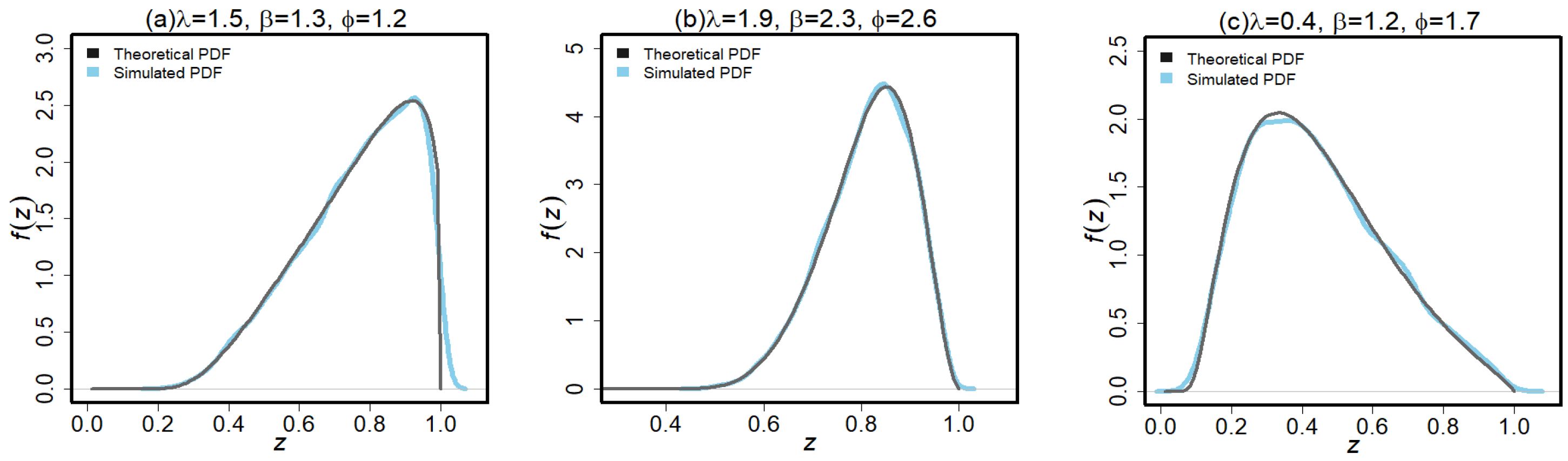The theoretical and simulated density functions of the HLUG-TI$\left(\breve{\mathsf{\Theta }}\right)$ model for given parameters choices are given in Figure 8. To obtain the bias average and MSE for each case, we execute the algorithm 10,000 times. The validity of the estimators is assessed using these biases and the MSE. The best estimator techniques are those that reduce MSE and estimator bias. The following stages are used to implement a simulation study for this purpose:

1. Generate ten thousand samples of size n from (4) for the HLUG-TI model. This work is done simply by the quantile function and generated data from the uniform distribution.

2. Evaluate the estimates for 10,000 samples, say $\left({\widehat{\lambda }}_i,{\widehat{\beta }}_i,{\widehat{\varphi }}_i\right)$ for $i=1,2,\dots ,$ 10,000.

3. Perform the biases and MSE calculations. The following formulas are used to accomplish these goals:

$$\begin{array}{ccc}\hfill Bia{s}_{\breve{\mathsf{\Theta }}}\left(n\right)& =& \frac{1}{10,000}\sum _{i=1}^{10,000}\left({\breve{\mathsf{\Theta }}}_i^{*}-\breve{\mathsf{\Theta }}\right),\hfill \end{array}$$

(87)

$$\begin{array}{ccc}\hfill MS{E}_{\breve{\mathsf{\Theta }}}\left(n\right)& =& \frac{1}{10,000}\sum _{i=1}^{10,000}{\left({\breve{\mathsf{\Theta }}}_i^{*}-\breve{\mathsf{\Theta }}\right)}^2,\hfill \end{array}$$

(88)

where $\breve{\mathsf{\Theta }}=\left(\lambda ,\beta ,\varphi \right).$

4. For all estimation approaches, these procedures were repeated for $n=30,34,\dots ,600,$ with the aforementioned parameters. To determine the value of estimators, we used R’s optim function. In Figure 9, Figure 10 and Figure 11, the simulation outcomes are shown graphically. As seen in Figure 9, Figure 10 and Figure 11, these biases and MSEs change with regard to n (left and right panels).

The pattern in the MSEs indicates consistency because the MSEs converge to zero when the value of n increases, but we can conclude that the estimators have the property of asymptotic unbiasedness because as n increases, the bias goes to zero. From Figure 9, Figure 10 and Figure 11, the following observations can be extracted:

• For all estimation techniques, the bias of $\widehat{\lambda },\widehat{\beta }$ and $\widehat{\varphi }$ reduces as n increases.
• For all methods, the biases of $\widehat{\lambda }$ are generally positive.
• For all methods, the negative biases of $\widehat{\beta }$ and $\widehat{\varphi }$ are also observed.
• The bias of parameter $\lambda$ is larger than parameter $\beta$ and $\varphi$.
• Under all of the methods, the MSEs of $\widehat{\lambda }$ seem larger.
• Based on Figure 9, Figure 10 and Figure 11, the MLE method has the minimal amount of MSE; however, for a large sample size, all methods have almost the same behavior and converge to zero as expected.
• Using the entries of the graphical study for different parametric combinations, we can conclude that the MLE method outperforms all other estimation methods with an overall minimum amount of bias and MSE. Therefore, depending on the simulation study, the MLE method performs best for HLUG-TI distribution.

A general conclusion from the figures is that, for all approaches, bias and MSE for three parameters converge to zero as sample sizes increase. This demonstrates the reliability of these estimating strategies for the HLUG-TI$\left(\breve{\mathsf{\Theta }}\right)$ model’s parameters.

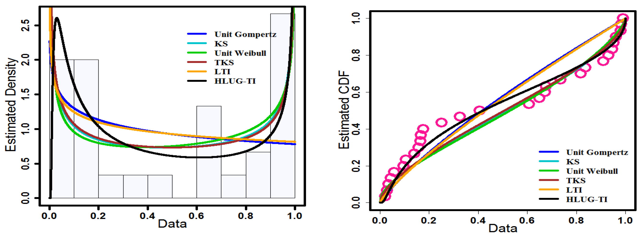
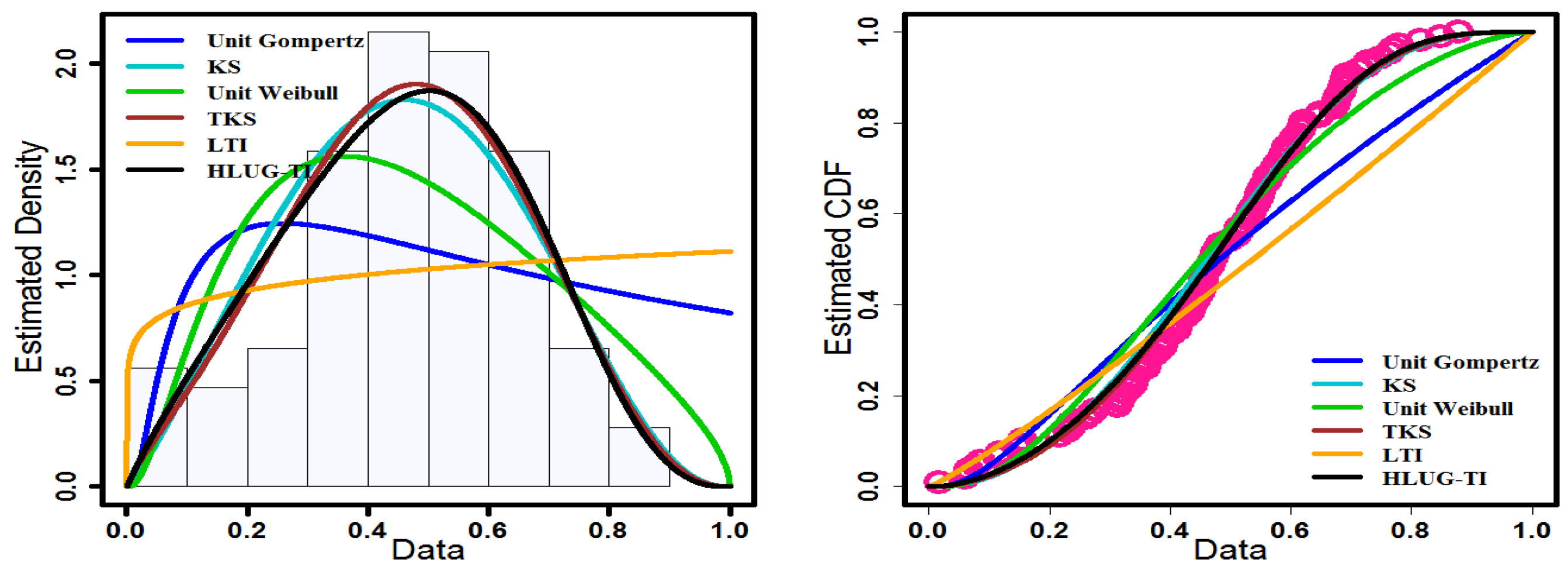
7. Real Data Applications

In this section, we implement the HLUG-TI$\left(\breve{\mathsf{\Theta }}\right)$ model on practical datasets to demonstrate its versatility in comparison to a set of competing models. The objective of the HLUG-TI$\left(\breve{\mathsf{\Theta }}\right)$ model is to provide an alternate distribution to fit the unit interval data in comparison to other distributions found in the literature. The first dataset from the reliability engineering field consists of 20 observations of the failure times of mechanical components [24]. The second dataset relates to the total milk yield in the first birth of 107 cows at the Carnauba farm in Brazil. These data are available in these studies [25,26]. To conclude, for the two datasets, the HLUG-TI model shows to be the most suitable model, demonstrating its applicability in a realistic environment. The parameters of the models were estimated by the MLE method [27,28].

Now, we compare the HLUG-TI model to a set of competing models, which are as follows: unit-Gompertz [1], Kumaraswamy [29], unit-Weibull [30], transmuted Kumaraswamy (TKSW, [31]) and Lehmann Type-I (LTI, [32]) distributions. To determine the rationality of utilizing the HLUG-TI distribution to fit these datasets, the goodness-of-fit measures the following: Akaike information criterion (AIC), Bayesian information criterion (BIC), Cramer–von Mises (CVM) and Anderson–Darling (AD). Consequently, the Kolmogorov–Smirnov (K-S) test is considered, and the P-value (PV) of K-S test was specified to compare models. The K-S statistic of the distance between the fitted and empirical distribution functions is one of the most widely used goodness-of-fit test statistics for determining how well a random sample’s distribution agrees with a theoretical distribution. The best model has high PV and low AIC, BIC, CVM, and AD values [33]. An overview of the estimated MLEs and fitted information criteria for both data sets using various models can be seen in

Table 2. MLEs and SEs of the parameters of considered distribution for Data Set I.

Distributions	MLEs	Standard Errors
Unit-Gompertz $\left(\eta ,b\right)$	$22.4727,$ $0.0348$	$67.0628,$ $0.0994$
KSwamy$\left(\alpha ,\beta \right)$	$0.5875,$ $0.6115$	$0.1607,$ $0.1339$
Unit-Weibull$\left(\alpha ,\beta \right)$	$0.9688,$ $0.7394$	$0.1874,$ $0.1125$
HLUG-TI$\left(\lambda ,\beta ,\varphi \right)$	$0.1081,$ $0.8046,$ $0.4845$	$0.1553,$ $0.3711,$ $0.1301$
TKSW$(\alpha ,\beta ,\lambda )$	$0.6091,$ $0.5854,$ $0.1246$	$0.1782,$ $0.1750,$ $0.4948$
LTI$\left(\alpha \right)$	$0.8166$	$0.1491$

,

Table 3. MLEs and SEs of the parameters of considered distribution for Data Set II.

Distributions	MLEs	Standard Errors
Unit-Gompertz $\left(\eta ,b\right)$	$2.1193,0.3878$	$0.8683,0.1145$
KSwamy$\left(\alpha ,\beta \right)$	$2.1949,$ $3.4363$	$0.2224,$ $0.5820$
Unit-Weibull$\left(\alpha ,\beta \right)$	$0.9846,$ $1.5620$	$0.1015,$ $0.1064$
HLUG-TI$\left(\lambda ,\beta ,\varphi \right)$	$70.70084,$ $0.0252,$ $3.7046$	$62.5229,$ $0.0216,$ $0.5616$
TKSW$(\alpha ,\beta ,\lambda )$	$1.8231,3.4361,-0.5608$	0.2735, 0.5622, 0.2246
LTI$\left(\alpha \right)$	$1.1123$	$0.1075$

,

Table 4. Values of the considered goodness-of-fit measures for Data I.

Distribution	AIC	BIC	HQIC	−LL	$\mathit{K}-\mathit{S}$	PV
Unit-Gompertz $\left(\eta ,b\right)$	2.6975	5.4999	3.5940	−0.6513	0.1955	0.1766
KSwamy$\left(\alpha ,\beta \right)$	−3.0050	−0.2026	−2.1085	−3.5025	0.1600	0.3850
Unit-Weibull$\left(\alpha ,\beta \right)$	−1.7447	1.0577	−0.8482	−2.8723	0.1664	0.3393
HLUG-TI$\left(\lambda ,\beta ,\varphi \right)$	−5.9084	−1.7048	−4.5637	−5.9542	0.11441	0.7857
TKSW$\left(\alpha ,\beta ,\lambda \right)$	−1.0692	3.1344	0.2756	−3.5346	0.1568	0.4097
LTI$\left(\alpha \right)$	0.6801	2.0813	1.1284	−0.6599	0.1926	0.1895

and

Table 5. Values of the considered goodness-of-fit measures for Data II.

Distribution	AIC	BIC	HQIC	−LL	$\mathit{K}-\mathit{S}$	PV
Unit-Gompertz $\left(\eta ,b\right)$	−6.977409	−1.631752	−4.810351	−5.488705	0.18347	0.001488
KSwamy$\left(\alpha ,\beta \right)$	−46.78936	−41.4437	−44.6223	−25.39468	0.07625	0.5626
Unit-Weibull$\left(\alpha ,\beta \right)$	−29.8423	−24.49664	−27.67524	−16.92115	0.12061	0.08891
HLUG-TI$\left(\lambda ,\beta ,\varphi \right)$	−48.86908	−40.85059	−45.61849	−27.43454	0.0692	0.6851
TKSW$\left(\alpha ,\beta ,\lambda \right)$	−48.09763	−40.07914	−44.84704	−27.04881	0.0670	0.6835
LTI$\left(\alpha \right)$	0.8290953	3.501924	1.912625	−0.5854524	0.24183	0.0000

. The values of the above measures suggest that the HLUG-TI model is a suitable competitor to other competitive distributions, and it also has the best fit among them. The histograms of the data sets and the fitted density function, as well as the plot of the empirical and estimated CDF of these fitted distributions, are shown in Figure 12 and Figure 13 to help determine if the HLUG-TI model is suitable. 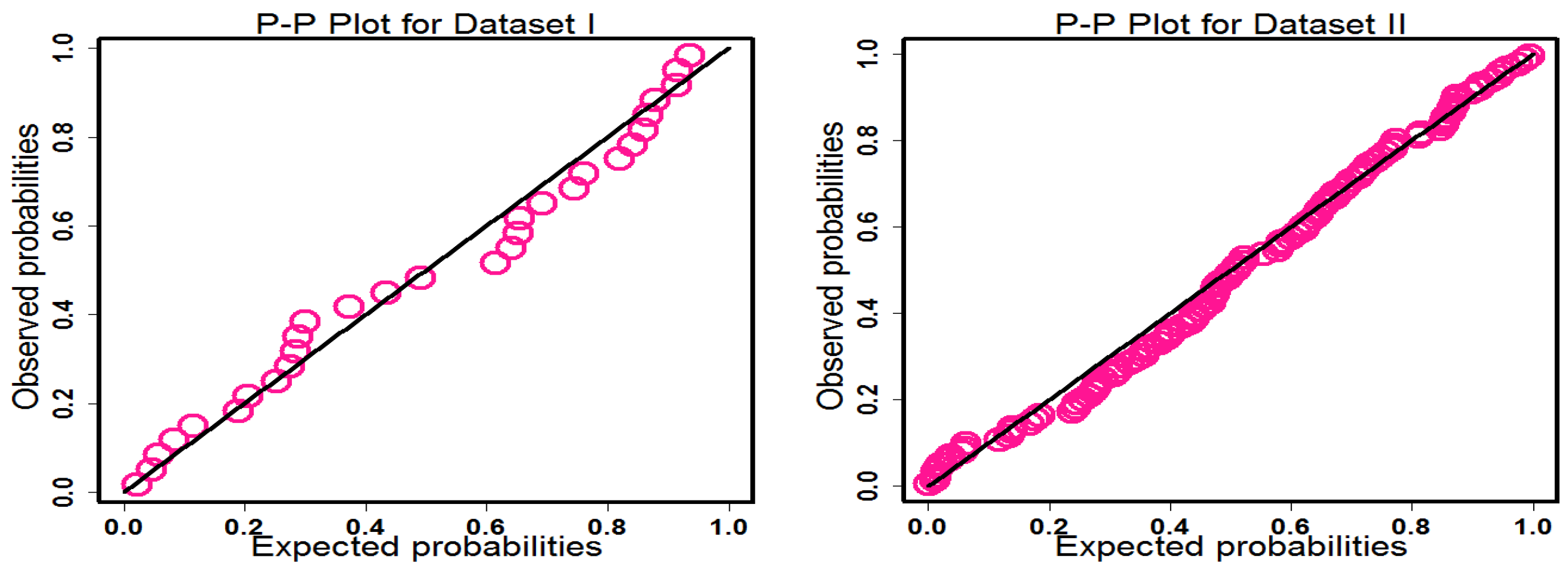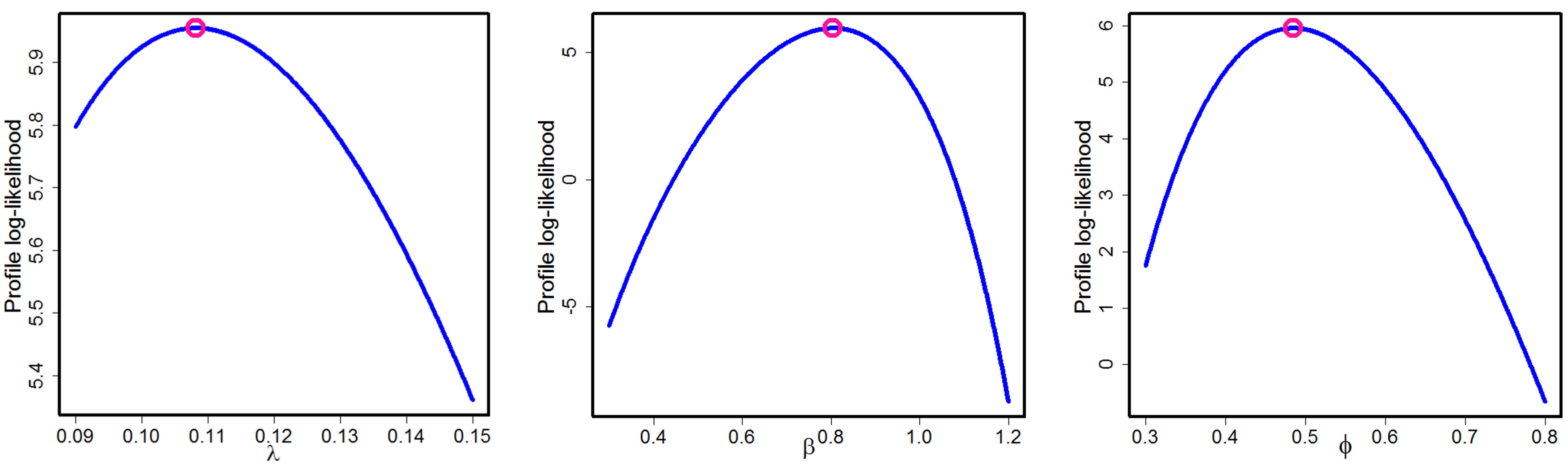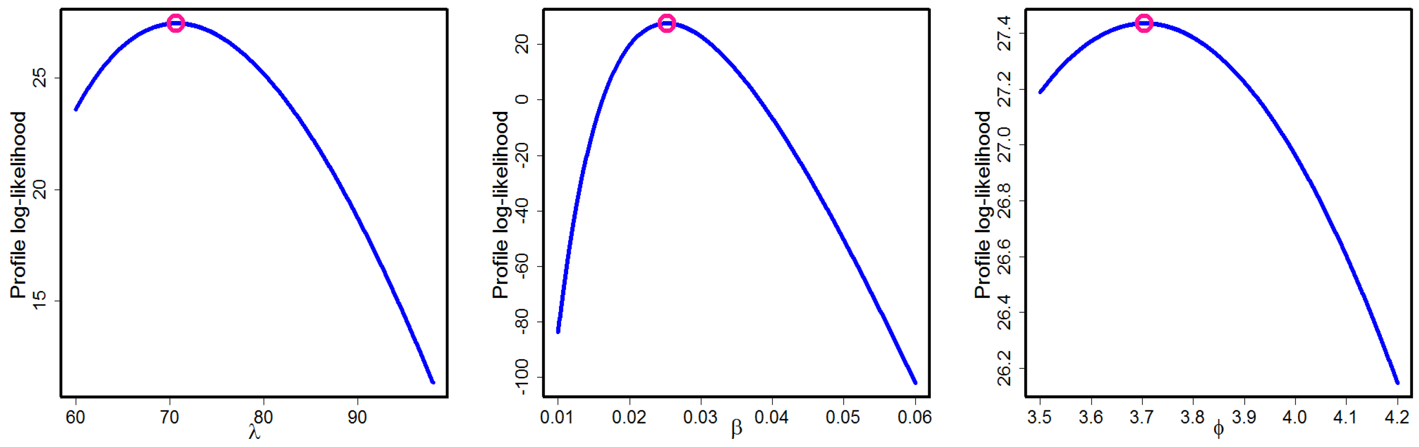Figure 14 also shows the P-P plots for the HLUG-TI model. Based on such graphical methods, we can suggest that the HLUG-TI model is a better model for the data sets under consideration. The profile likelihood functions of parameters of HLUG-TI for both data sets are presented in Figure 15 and Figure 16.

8. Conclusions

In this study, we present a novel three-parameter model called the half-logistic unit-Gompertz type-I (HLUG-TI) distribution, which generalizes the unit-Gompertz distribution. It is competent at modeling data with increasing, bathtub, unimodal, and then bathtub hazard rate functions. Some mathematical properties of the introduced model are derived. The HLUG-TI parameters are estimated using six estimation methods, namely the maximum likelihood, least squares, weighted least-squares, Cramér–von Mises, Anderson–Darling, and right-tail Anderson–Darling estimators. The simulation study is conducted to explore the efficiency of these estimators and to provide a guideline for applied statisticians and engineers in choosing the best estimation method. Further, the importance of the HLUG-TI model is utilized by two real data applications. The goodness-of-fit for the two data sets show that the introduced model outperforms the four competitors, all of which are based on the bounded interval.

References

1. Mazucheli, J.; Menezes, A.F.; Dey, S. Unit-Gompertz Distribution with Applications. Statistica 2019, 79, 25–43. [Google Scholar] [CrossRef]
2. Jha, M.K.; Dey, S.; Tripathi, Y.M. Reliability estimation in a multicomponent stress-strength based on unit-Gompertz distribution. Int. J. Qual. Reliab. Manag. 2019, 37, 428–450. [Google Scholar] [CrossRef]
3. Kumar, D.; Dey, S.; Ormoz, E.; MirMostafaee, S.M.T.K. Inference for the unit-Gompertz model based on record values and inter-record times with an application. Rend. Circ. Mat. Palermo Ser. 2020, 69, 1295–1319. [Google Scholar] [CrossRef]
4. Jha, M.K.; Dey, S.; Alotaibi, R.M.; Tripathi, Y.M. Reliability estimation of a multicomponent stress-strength model for unit Gompertz distribution under progressive Type II censoring. Qual. Reliab. Eng. Int. 2020, 36, 965–987. [Google Scholar] [CrossRef]
5. Anis, M.Z.; De, D. An expository note on unit-Gompertz distribution with applications. Statistica 2020, 80, 469–490. [Google Scholar]
6. Eugene, N.; Lee, C.; Famoye, F. Beta-normal distribution and its applications. Commun. Stat. Theor. Meth. 2002, 31, 497–512. [Google Scholar] [CrossRef]
7. Zografos, K.; Balakrishnan, N. On families of beta and generalized gamma-generated distributions and associated inference. Stat. Methodol. 2009, 6, 344–362. [Google Scholar] [CrossRef]
8. Cordeiro, G.M.; de Castro, M. A new family of generalized distributions. J. Stat. Comput. Simul. 2011, 81, 883–898. [Google Scholar] [CrossRef]
9. Alzaatreh, A.; Ghosh, I. On the Weibull-X family of distributions. J. Stat. Theory Appl. 2015, 14, 169–183. [Google Scholar] [CrossRef] [Green Version]
10. Tahir, M.H.; Cordeiro, G.M.; Alizadeh, M.; Mansoor, M.; Zubair, M.; Hamedani, G.G. The odd generalized exponential family of distributions with applications. J. Stat. Distrib. Appl. 2015, 2, 1. [Google Scholar] [CrossRef] [Green Version]
11. Muhammad, M. Poisson-odd generalized exponential family of distributions: Theory and applications. Hacet. J. Math. Stat. 2018, 47, 1652–1670. [Google Scholar] [CrossRef]
12. Cordeiro, G.M.; Alizadeh, M.; Diniz Marinho, P.R. The type I half-logistic family of distributions. J. Stat. Comput. Simul. 2015, 86, 707–728. [Google Scholar] [CrossRef]
13. Dey, S.; Moala, F.A.; Kumar, D. Statistical properties and different methods of estimation of Gompertz distribution with application. J. Stat. Manag. Syst. 2018, 21, 839–876. [Google Scholar] [CrossRef] [Green Version]
14. Dey, S.; Alzaatreh, A.; Zhang, C.; Kumar, D. A new extension of generalized exponential distribution with application to ozone data. Ozone Sci. Eng. 2017, 39, 273–285. [Google Scholar] [CrossRef]
15. Nair, N.U.; Sankaran, P.G.; Balakrishnan, N. Quantile-Based Reliability Analysis; Springer Science & Business Media: Berlin/Heidelberg, Germany, 2013. [Google Scholar]
16. Olver, F.W.J.; Daalhuis, A.B.O.; Lozier, D.W.; Schneider, B.I.; Boisvert, R.F.; Clark, C.W.; Miller, B.R.; Saunders, B.V. (Eds.) NIST Digital Library of Mathematical Functions. Release 1.0.19 of 2018-06-22. Available online: http://dlmf.nist.gov/ (accessed on 21 March 2022).
17. Tippett, L.H. On the extreme individuals and the range of samples taken from a normal population. Biometrika 1925, 17, 364–387. [Google Scholar] [CrossRef]
18. Silva, G.O.; Ortega, E.M.; Cordeiro, G.M. The beta modified Weibull distribution. Lifetime Data Anal. 2010, 16, 409–430. [Google Scholar] [CrossRef]
19. Anderson, T.W.; Darling, D.A. Asymptotic theory of certain “goodness of fit” criteria based on stochastic processes. Ann. Math. Stat. 1952, 23, 193–212. [Google Scholar] [CrossRef]
20. Anderson, T.W.; Darling, D.A. A test of goodness of fit. J. Am. Stat. Assoc. 1954, 49, 765–769. [Google Scholar] [CrossRef]
21. Pettitt, A.N. A Two-Sample Anderson–Darling Rank Statistic. Biometrika 1976, 63, 161. [Google Scholar]
22. Stephens, M.A. Components of goodness-of-fit statistics. Ann. Inst. Henri Poincare B 1974, 10, 37–54. [Google Scholar]
23. Boos, D.D. Minimum distance estimators for location and goodness of fit. J. Am. Stat. Assoc. 1981, 76, 663–670. [Google Scholar] [CrossRef]
24. Murthy, D.P.; Xie, M.; Jiang, R. Weibull Models; John Wiley & Sons: Hoboken, NJ, USA, 2004. [Google Scholar]
25. Cordeiro, G.M.; dos Santos Brito, R. The beta power distribution. Braz. J. Probab. Stat. 2012, 26, 88–112. [Google Scholar]
26. Brito, R.S. Estudo de Expansoes Assintoticas. Avaliacao Numnerica de Momentos das Distribuicoes Beta Generalizadas, Aplicaoes em Modelos de Regressao e Analise Discriminante. Master’s Thesis, Universidade Federal Rural de Pernambuco, Recife, Brazil, 2009. [Google Scholar]
27. Shafiq, A.; Lone, S.A.; Sindhu, T.N.; El Khatib, Y.; Al-Mdallal, Q.M.; Muhammad, T. A new modified Kies Fréchet distribution: Applications of mortality rate of COVID-19. Results Phys. 2021, 28, 104638. [Google Scholar] [CrossRef]
28. Sindhu, T.N.; Shafiq, A.; Al-Mdallal, Q.M. On the analysis of number of deaths due to COVID-19 outbreak data using a new class of distributions. Results Phys. 2021, 21, 103747. [Google Scholar] [CrossRef]
29. Jones, M.C. Kumaraswamy’s distribution: A beta-type distribution with some tractability advantages. Stat. Methodol. 2009, 6, 70–81. [Google Scholar] [CrossRef]
30. Mazucheli, J.; Menezes, A.F.B.; Fernandes, L.B.; de Oliveira, R.P.; Ghitany, M.E. The unit-Weibull distribution as an alternative to the Kumaraswamy distribution for the modeling of quantiles conditional on covariates. J. Appl. Stat. 2020, 47, 954–974. [Google Scholar] [CrossRef] [PubMed]
31. Khan, M.S.; King, R.; Hudson, I.L. Transmuted kumaraswamy distribution. Stat. Transit. New Ser. 2016, 17, 183–210. [Google Scholar] [CrossRef] [Green Version]
32. Lehmann, E.L. The power of rank tests. Ann. Math. Stat. 1953, 24, 23–43. [Google Scholar] [CrossRef]
33. Shafiq, A.; Sindhu, T.N.; Lone, S.A.; Hassan, M.K.; Nonlaopon, K. Mixture of Akash Distributions: Estimation, Simulation and Application. Axioms 2022, 11, 516. [Google Scholar] [CrossRef]
Figure 1. Variations of PDF of the HLUG-TI for different parameter values.
Mathematics 11 01007 g001
Figure 2. Variations of HRF of the HLUG-TI for different parameter values.
Mathematics 11 01007 g002
Figure 3. Variations of PDF and HRF of the HLUG-TI at different values of parameters.
Mathematics 11 01007 g003
Figure 4. Effects of skewness and kurtosis of HLUG-TI for certain values of parameters.
Mathematics 11 01007 g004
Figure 5. Plots of skewness of HLUG-TI Θ ˘  for certain parameter values.
Mathematics 11 01007 g005
Figure 6. Plot of kurtosis of HLUG-TI Θ ˘  for certain parameter values.
Mathematics 11 01007 g006
Figure 7. Plot of median of HLUG-TI Θ ˘  for certain parameter values.
Mathematics 11 01007 g007
Figure 8. Plot of theoretical and simulated PDF of HLUG-TI for certain parameter values.
Mathematics 11 01007 g008
Figure 9. Plots of biases and MSEs for the parameters  λ = 1.5 ,   β = 1.3  and  ϕ = 1.2  of HLUG-TI model.
Mathematics 11 01007 g009aMathematics 11 01007 g009b
Figure 10. Plots of biases and MSEs for the parameters  λ = 1.9 ,   β = 2.3  and  ϕ = 2.6  of HLUG-TI model.
Mathematics 11 01007 g010
Figure 11. Plots of biases and MSEs for the parameters  λ = 0.4 ,   β = 1.2  and  ϕ = 1.7  of HLUG-TI model.
Mathematics 11 01007 g011
Figure 12. Estimated densities and empirical (left) and estimated CDF (right) for the data set I.
Mathematics 11 01007 g012
Figure 13. Estimated densities and empirical (left) and estimated cdf (right) for Data Set II.
Mathematics 11 01007 g013
Figure 14. P-P plot for Data Sets I and II.
Mathematics 11 01007 g014
Figure 15. Unimodal profile likelihood functions of parameters of HLUG-TI for Data I.
Mathematics 11 01007 g015
Figure 16. Unimodal profile likelihood functions of parameters of HLUG-TI for Data II.
Mathematics 11 01007 g016